Secondary Heavy Quark Production in Jets through Mass Modes
Abstract
We present an effective field theory method to determine secondary massive quark effects in jet production taking the thrust distribution for collisions in the dijet limit as a concrete example. The method is based on the field theoretic treatment of collinear and soft mass modes which have to be separated coherently from the collinear and ultrasoft modes related to massless quarks and gluons. For thrust the structure of the conceptual setup is closely related to the production of massive gauge bosons and involves four different effective field theories to describe all possible kinematic situations. The effective field theories merge into each other continuously and thus allow for a continuous description from infinitely heavy to arbitrarily small masses keeping the exact mass dependence of the most singular terms treated through factorization. The mass mode field theory method we present here is in the spirit of the variable fermion number scheme originally proposed by Aivazis, Collins, Olness and Tung and can also be applied in hadron collisions.
I Introduction
By now jet physics has reached a high level of precision allowing for an accurate description of the strong interaction. Fundamental parameters of QCD such as the strong coupling constant as well as nonperturbative properties of hadrons like parton distribution functions can be determined with a continuously improved accuracy from high precision data samples. On the theoretical side this has been possible thanks to high order loop calculations and the summation of large logarithmic terms. Computations of jet cross sections for massless quarks belong to the well known and unambiguously defined exercises in perturbative QCD based on a number of rigorous factorization proofs. On the other hand, as far as massive quarks are concerned it is fair to say that their treatment is not coherent throughout the literature. Different schemes for massive quarks exist which differ in the resummation of logarithms and in the inclusion of formally subleading contributions. An approach capable of describing quark mass effects starting in principle from very small masses when the quarks are inside hadrons and stretching up to ultra-heavy masses in the decoupling limit was provided by Aivazis, Collins, Olness and Tung (ACOT) [1, 2]. Their variable fermion number scheme is based on the separation of close-to-mass-shell and off-shell modes. At LO in the inverse hard scattering scale expansion, it allows to factorize infrared-safe hard coefficient corrections from low-energy parton distribution terms involving logarithmic mass effects. In this respect the concept behind the ACOT scheme is along the lines of effective field theory methods such as the soft-collinear effective theory (SCET) framework [3, 4] and can be readily incorporated into it. As we show in this paper, the resulting effective theory framework can be based on the inclusion of collinear and soft ”mass modes”11 1 This differs from the terminology used in Refs. [5] and [6] where only the soft massive modes were referred to as the mass modes. together with the existing collinear and ultrasoft massless partonic modes. While the collinear and ultrasoft massless partonic modes typically have different invariant masses depending on the observable under consideration, the collinear and soft mass modes also contain fluctuations related to their intrinsic mass scale. This can lead to complicated patterns of scale hierarchies that might even vary substantially within a single distribution.

In this and a subsequent paper we apply the mass mode SCET concept to describe the secondary production of massive quarks in the thrust distribution. While we aim for the description of thrust, the described method is general and can be applied with possible adaptions to other processes as well. Recently, a factorization approach was derived within SCET that can be applied for thrust induced by primary heavy quarks, i.e. by heavy quarks that are produced directly from the hard jet current [5, 6]. For the description of primary heavy quarks the mass modes are involved as well, but they play a more simplistic role since massless collinear modes are directly tied to the massive collinear modes and soft mass modes turn out to only lead to virtual effects. So the resulting situation is almost identical to the one in massless SCET. For secondary heavy quark production, i.e. for heavy quarks produced from gluon radiation off primary massless quarks, Fig. 1, the collinear and ultrasoft massless as well as massive modes can all constitute independent degrees of freedom. Each of them can contribute to dynamical thresholds effects as well as to virtual contributions. Here the dynamical mass effects enter in different ways depending on the relation of the mass scale to the kinematic scales relevant for massless quark production. Depending on the mass value the scale hierarchies can vary substantially requiring different types of effective field theory setups that have to merge into each other in a connected way to allow for a continuous description of the distribution. The secondary quark mass effects in thrust thus represent a non-trivial prototypical showcase for the mass mode concept.
Concerning the numerical size, the effects from secondary heavy quarks in thrust are in fixed-order perturbation theory and certainly small if the hard scale is much bigger than the heavy quark mass. Nevertheless the numerical effects involve logarithms related to renormalization evolution with variable flavor number already at the leading-logarithmic level and are important if the hard scale is only a few times larger than the mass. They are certainly essential for a precision analysis of event shapes for GeV concerning the description of bottom mass effects. So studying the secondary heavy quark effects in thrust is also of phenomenological interest.
An interesting conceptual issue, which can also lead to considerable computational simplifications, is that the description of secondary massive quarks radiation is closely tied to radiation of massive gauge bosons. All non-trivial conceptual aspects and also some computational issues can be conveniently addressed considering the setup with massive gauge bosons which we mostly concentrate on in this first paper. Details on the computation of the effects of secondary massive quarks and extensive numerical studies are postponed to Ref. [7].
This paper is organized as follows. In Sec. II we explain the outline and the scope of the mass mode method. We also show how secondary massive quark radiation is tied up to the description of massive gauge bosons. The required effective field theory framework can be conveniently formulated concentrating on collinear and soft massive gauge boson radiation as a placeholder. Essentially all non-trivial conceptual and technical issues can be discussed and handled with massive gauge bosons. In Sec. III we review the massless factorization theorem for the thrust differential cross section. In Sec. IV, which is the central section of this paper, we explain our theoretical setup to describe modifications in the factorization theorem due to secondary massive particles described by mass modes, and we show the results for massive gauge bosons with vector coupling. Here we also address how our approach achieves a continuous description of the full mass-dependence of the most singular terms in the dijet limit covering all possible hierarchies, and we discuss the role of mass corrections at the transition points between the different scenarios. Details on the actual calculations are given in Sec. V for the full theory results and in Sec. VI in the effective theory framework. As an outlook we describe briefly the two-loop computations required for secondary massive quarks in Sec. VII and show the impact of our results on the thrust distribution. Finally in Sec. VIII we summarize and conclude.
II The Outline
We consider the effect of secondary massive quarks in the thrust distribution for massless primary quark production, . For thrust we use the definition
| (1) |
where is the thrust axis and the sum is performed over all final state particles with momenta and energies .22 2 We define the thrust variable normalized with the c.m. energy , which is the sum of all energies and also agrees with the variable 2-jettiness [8]. For massless decay products this agrees with the common definition, which is normalized to the sum of momenta . The most singular terms for small (i.e. in the dijet limit) are governed by a factorization theorem that separates the dynamical fluctuations at the center-of-mass energy (hard scale), the typical invariant mass of each of the jets (jet scale) and the typical energy of large angle ultrasoft radiation (ultrasoft scale), where the power counting parameter in the tail region of the thrust distribution. For the effects of the massive quark decouple and the factorization theorem for the singular partonic cross-section adopts the well known form for massless quarks [5]. Schematically the form is
| (2) |
Here denotes the hard contribution, the jet function describing collinear fluctuations, which is convoluted with the soft function arising from soft large angle radiation. To avoid large logarithms each term is evaluated at its characteristic renormalization scale, so that for the hard factor, for the collinear jet function and for the soft function. Large logarithms between these scales are summed by the renormalization group factors which are implied.

In order to determine the effects of secondary radiation of heavy quarks through gluon splitting (Fig. 1) one has to deal with two issues: (i) the separation of dynamical modes depending on the relation of the mass with respect to the hard, jet and ultrasoft scales and (ii) the calculation of the secondary massive quark contributions in connection with the appropriate number of flavors contributing to the renormalization group evolution. For jet observables and quantities depending only on the invariant mass of the secondary fermion pair the two issues can be completely disentangled. This is achieved by using the fact that the quark pair polarization correction to the gluon propagator can be expressed as a dispersion integral of a massive gluon propagator with the absorptive part of the quark-vector current correlator (see Fig. 2). Using this dispersion integral method [9, 10, 11] we can set up the conceptual formalism to describe the secondary massive quark pair radiation and to separate the massive modes in connection to the massless collinear and soft modes by first considering real and virtual radiation of “gluons” with mass , as shown in Fig. 3.

All conceptual issues concerning the separation of modes, the determination of matching conditions and of matrix elements within the context of SCET can be conveniently discussed with the massive gauge bosons.
One has to consider collinear (for each jet direction) as well as soft “gluon” modes with mass , all of which can have mass-shell fluctuations of equal typical virtuality of in addition to fluctuations at the hard, jet and ultrasoft scale depending on the kinematic situation. In contrast, massless collinear and ultrasoft modes live exclusively at the jet and ultrasoft scale, respectively, and their (zero) mass-shell fluctuations do not need to be considered for the separation of modes. After having carried out all calculations with the massive “gluons”, the effects from secondary massive quark radiation are obtained by the dispersion integration over the gauge boson mass according to Fig. 2. The dispersion integration can be carried out either in the unsubtracted or subtracted versions depending on whether the massive quark flavor gives a UV divergence and contributes to the RG-evolution or whether it is integrated out and does not contribute to the RG-evolution.
In this paper we mostly concentrate on the conceptual aspects related to the collinear and soft gauge bosons with mass and on their effects in thrust. We aim at a continuous description of the most singular terms treated in the factorization theorem for all mass values from , where decoupling takes place, down to the limit , where the formalism continuously interpolates to the well-known case of a massless gluon. The linearity of the dispersion integration entails that the continuity is carried over also to the contributions coming from the secondary massive quarks. The continuity of the theoretical description as a function of , the mass and the external kinematical variables (which is thrust in our concrete application) is particularly important, since different hierarchies between the mass scale and the jet and ultrasoft scales can arise within a single spectrum when the kinematic variables are varied within their allowed kinematic ranges.
We stress that the mass mode method we present here is not tied to separating the problem into a treatment of massive gauge bosons and dispersion integrations. Once the field theoretic setup is identified (where the use of massive gauge bosons might certainly serve as a useful guideline) the approach can be formulated right away in terms of massive quark modes. In general this can be even necessary when jet observables are considered that do not depend in a universal way on the invariant mass of the quark pair. However, in cases where the dispersion method can be applied the results for the massive gauge bosons are universal and results for other types of secondary massive particles (scalars, vector bosons) can be readily obtained simply by using the respective version of the dispersion relation. Moreover in many non-universal cases the computationally easier dispersion method can be used to at least correctly determine ultra-violet (UV) divergent and/or infrared (IR) singular terms, such that the remaining finite terms might not need to be carried out with regulators. For thrust this is the case concerning large angle soft radiation.
An interesting technical aspect of computations with mass modes is that usual dimensional regularization is not capable of separating the mass-shell contributions coming from the collinear and soft sectors, see e.g. Refs. [12, 13, 14]. This leads to unregularized divergences in the respective collinear and soft diagrams which appear to be related to the fact that dimensional regularization regularizes with respect to virtualities, whereas the mass-shell fluctuations from the collinear and soft mass modes are separated only by a boost. As we demonstrate in this work, these singularities drop out of the properly defined matrix elements and matching coefficients, so that in principle no regularization scheme other than dimensional regularization is necessary. Using the mass mode massive gauge bosons and the dispersion method allows for a simple computational scheme to deal with these singularities because the singular terms can already be canceled at the level of one-loop diagrams. This can also lead to substantial technical simplifications in cases where the secondary massive quarks enter an observable in a non-universal way. The singularities appearing in the mass-shell contributions of the collinear and soft mass modes, however, lead to large logarithmic terms in the mass-shell matching corrections that arise when the mass modes are integrated out. These logarithms can in general not be summed up within the renormalization evolution carried by the -dependence within dimensional regularization. Recently, several approaches to handle the summation of these ”rapidity logarithms” have been discussed in the literature [15, 16, 17, 18]. Since the methods to treat the rapidity logarithms are orthogonal to the renormalization flow governed by the -dependence, they can be readily implemented into our mass mode formalism through a separate procedure. We adopt a method based on the “rapidity renormalization group“ [18], and using an analytic regulator [16]. The outcome is a simple exponentiation of logarithms in the mass mode matching conditions. Our treatment represents a novel non-trivial application of summing rapidity logarithms worth to be studied by itself.
We note that our effective theory setup involving the mass mode gauge bosons entails that they are distinct degrees of freedom and exist in parallel to the common massless collinear and ultrasoft gluons. While we primarily give them the role of placeholders for the mass mode collinear quarks (and the collinear gluonic modes they can interact with) the calculations we carry out in this work can be of direct interest by themselves and might well serve for concrete applications for example related to the electroweak theory. To be specific the mass mode gauge bosons might be considered within the context of an additional spontaneously broken SU(2) gauge theory where all SU(2) gauge bosons get a common mass from a Higgs in the fundamental representation. Similar to Refs. [19, 12, 13] we write the corresponding SU(2) group theory factors using , and and denote the gauge coupling as with . This agrees with our notation for the QCD results and facilitates the interpretation of the results for the dispersion integration used to implement the corrections due to the gluon splitting.
As a final introductory remark we note that for the calculations of the secondary massive quark effects all computations are performed in dimensional regularization. Since in this paper we mostly focus on the conceptual field theory and computational issues related to the massive gauge bosons we present all results in the limit to facilitate the discussions. Details on the -dimensional results together with the corrections caused by the secondary massive quarks are treated in a subsequent publication [7].
III The massless factorization theorem
In this section we briefly review the known massless factorization theorem for thrust to set up our notations and collect the perturbative QCD results at one loop. The inclusion of the mass modes modifies the form of the massless factorization theorem, and we show in the next sections that the various mass mode contributions to the factorization theorem interpolate continuously to the respective massless contributions in the limit . The factorization theorem sums large logarithms in the terms of the thrust distribution that are singular in the dijet limit. The thrust distribution reads [5]
| (3) |
where denotes the total partonic cross-section at tree-level, is the hard current matching condition, the thrust jet function and the thrust soft function. Large logarithms between the characteristic scales of each sector, , and , and the final renormalization scale are summed by the evolution factors , and satisfying the renormalization group equations
| (4) | ||||
| (5) | ||||
| (6) |
The superscript in the evolution factors as well as the subscript in the matrix elements indicate an expression in the massless theory without mass modes. The choice of is arbitrary, and the dependence on cancels exactly working at a particular order. In this work we adopt the choice , such that the evolution factor and can be dropped from Eq. (3). The fact that other choices for can be implemented leads to interesting consistency conditions between the renormalization group factors which have been discussed in detail in Ref. [5]. We stress that beginning at all ingredients of the factorization theorem depend on the number of massless quarks . Currently , and the partonic contributions to are known up to [20, 21, 22, 23, 24] and the anomalous dimensions up to [20, 25], for even the corrections are available [26, 27] (see also Refs. [28, 29] for more detailed information).
The hard function is with the massless Wilson coefficient from matching SCET to QCD. At it reads (with )
| (7) |
The current divergences are canceled by the current renormalization factor
| (8) |
which yields for the leading order anomalous dimension
| (9) |
with and being the coefficients of the cusp and non-cusp anomalous dimensions.
The thrust jet function is obtained through a convolution of the hemisphere jet functions [6] for the two jet directions,
| (10) |
The jet functions and are matrix elements of collinear fields in SCET and describe the dynamics of the collinear degrees of freedom. The collinear jet function is defined as
| (11) |
where the jet fields denote quark fields multiplied by collinear Wilson lines and the invariant mass is . All color and spin indices are traced implicitly. For further details and the definition for we refer to Ref. [5].
The renormalized expression for at one loop order reads
| (12) |
with . The one-loop renormalization factor for the massless jet function reads
| (13) |
which yields for the leading order anomalous dimension
| (14) |
with .
The thrust soft function describes ultrasoft radiation between the two jets and is based on a hemisphere definition,
| (15) |
where () is the momentum of the soft final state in the right (left) hemisphere and , are ultrasoft Wilson lines, i.e.
| (16) |
In the tail region where the ultrasoft scale is larger than the hadronic scale the thrust soft function factorizes into a perturbative partonic part and a nonperturbative hadronic part. In the following we will consider just the partonic soft function. The renormalized expression at is
| (17) |
with . Its renormalization factor at one loop reads
| (18) |
and yields for the leading logarithmic anomalous dimension
| (19) |
The anomalous dimensions (to any loop order) satisfy the consistency relation
| (20) |
IV The Mass Mode Setup
When mass modes are included, their intrinsic mass scale can enter the field theory setup in addition to the hard, jet and ultrasoft scales. It is convenient to define the ratio . There are different types of mass modes, collinear type modes and soft modes [14]. If kinematically allowed, the - and -collinear and soft mass modes have the scaling and the virtualities of their massless counterparts, but in addition we have to separately account for their mass-shell fluctuations. These have the scaling and for the - and -collinear mass mode, respectively, while soft mass modes have . It is the purpose of the mass mode formalism to separate these fluctuations in a systematic way when necessary.
The collinear massive quark interactions are determined from a massive quark collinear Lagrangian [30] which is a straightforward generalization of the massless collinear Lagrangian. The soft mass mode gauge bosons couple to collinear quarks through soft Wilson lines [5, 6] and the interactions of soft mass mode quarks and gluons among themselves is given by usual QCD interactions. An important aspect is that the mass mode collinear gauge bosons are defined with a soft mass mode-bin subtraction [14] in order to avoid double counting and maintain gauge invariance within each collinear sector.
The mass-shell fluctuations of the collinear and the soft mass modes are of the same order with and thus just separated by boosts and rapidity. They must be considered together with the collinear and ultrasoft virtualities given by the kinematics related to the scales and , respectively, with for thrust in the tail region. Depending on the relative size of , and , the mass modes therefore have to be treated differently with respect to the massless collinear and ultrasoft modes. This has an impact on the required matching and renormalization group calculations and therefore also on the form of the resulting factorization theorem. The different scenarios can be ordered according to where the mass scale is situated with respect to the jet and ultrasoft scales, see Fig. 4 and 5 for graphical illustrations. Each scaling situation corresponds in principle to a different EFT setup.


In the following we briefly summarize these different scenarios:33 3 For the effective field theory setup we require , but no large hierarchy concerning .
- I)
(): The mass is larger than the hard scale and the mass modes are not contained in SCET, but integrated out when SCET is matched to the full theory. So the factorization theorem is the one for massless fermions up to the hard current matching coefficient which acquires an additional contribution due to the mass modes. The mass effects decouple for .
- II)
(): In this scenario the mass is in between the hard scale and the jet scale. The mass mode effects are virtual because the jet scale , the typical invariant mass for real collinear particle radiation is below . However, the mass modes contribute to the matching condition at the scale and the evolution of the current for scales above . The mass-shell fluctuations are integrated out at the scale . The factorization theorem is the one for the massless quarks concerning jet and soft function but receives mass mode corrections in the matching and evolution of the production current. The matching condition of the production current at the hard scale has the correct massless limit for , since all mass-shell contributions have been removed from it in the matching procedure.
- III)
(): The mass is below the jet scale. Therefore massless and massive collinear modes both can fluctuate in the collinear sector yielding real and virtual contributions to the jet function. The soft mass modes only arise through their virtual effects since their interactions with collinear modes induce invariant masses above the jet scale. They contribute to the current matching and evolution together with the virtual mass-shell effects of the massive collinear modes exactly as in scenario II. Analogously to the previous scenario the mass-shell fluctuations are integrated out at the scale leading to an additional collinear mass mode matching condition. The soft function agrees with the one of the massless factorization theorem.
- IV)
(): When the mass is below the ultrasoft scale the mass-shell fluctuations of the mass modes merge into those of the massless quarks and gluons and in principle do not have to be separated. The collinear and soft fluctuations of the mass modes are treated at the same footing as those of the massless collinear and ultrasoft quarks and gluons. The soft mass modes adopt the same invariant mass scaling as the massless soft degrees of freedom. However, they still have a mass and this must be taken into account in the calculations. In this last scenario the mass-shell fluctuations are not integrated out and the factorization theorem has the form of the massless factorization theorem with the difference that the hard, jet and soft functions contain additional mass-dependent corrections which merge into the massless result for .
An important aspect is that the results in each scenario account for the full mass dependence of the singular contributions, which we do not further expand if the mass becomes smaller than any of the other kinematic scales. This yields a continuous description valid for any scaling between the mass and the hard, jet or soft scales and is important when scanning the thrust variable through the entire allowed spectrum. At this point one might worry whether the factorization theorems are subject to uncontrolled power corrections at the point where two scenarios are patched together. We show below that this is not the case and that there is no generic loss of precision where the transition between different scenarios is carried out.
We stress that the notation, the formulation of the factorization theorems and the organization of the RG evolution we employ is associated to the “top-down” evolution, where the scale is equal to the ultrasoft scale . Thus only the current and the jet function evolution factors and , respectively, appear in the factorization theorem. This also affects the interpretation and association of the mass-shell contributions which enter in the mass mode matching conditions discussed below. In this RG setting the jet and the soft functions do not receive any massive quark effects when the jet and ultrasoft scales, respectively, are below the mass mode matching scale. Alternative ways to describe RG-evolution related to different choices for are possible and have been discussed in Ref. [6]. There are consistency conditions that relate the RG-evolution and the mass mode matching factors for the different choices of . Since the mass appears as an additional scale in our mass mode setup, there are even more possibilities to set up RG-evolution. Therefore the consistency conditions become more involved, as they also entail relations between mass mode matching conditions and renormalization group evolution with different anomalous dimensions and varying flavor number. As an example, if is set to the hard scale, the jet and soft functions have to be evolved upwards to larger scales. In this RG setup the jet and soft functions can pick up virtual mass-shell corrections in case the mass threshold is crossed. We briefly come back to this issue in Sec. VI.3 and discuss the impact of these scenarios in more detail in Ref. [7].
In the subsections IV.1-IV.4 we give a more detailed description of the formalism and the results for each of the scenarios for the application to thrust. We also address why the transition between the various scenarios is continuous and why uncontrolled power corrections or power counting breaking effects do not arise. Overall this is conceptually related to the fact that the different effective theories are all matched to the singular contributions computed with the complete mass dependence in the full theory in an independent way and should not be thought of as being a sequence of effective theories matched to each other.
IV.1 Scenario I:
The massive gauge boson with vector coupling is integrated out at the hard scale , when SCET is matched to the full theory, yielding just a modification of the hard matching coefficient. It can be combined with the massless coefficient to give a new Wilson coefficient, which reads at one loop order
| (21) |
The massive contribution is computed from the full theory current form factor with a subtraction at (i.e. in the on-shell scheme which ensures decoupling) since the mass modes do not contribute to the SCET renormalization group evolution. At one-loop order reads [9, 31, 11]
| (22) |
with . In the limit the mass modes decouple, so for . In the small mass limit (which is not supposed to be taken in this scenario), on the other hand, we obtain
| (23) |
which yields unresummed large logarithms. Thus in scenario I the correct massless limit cannot be obtained in the hard Wilson coefficient of Eq. (21), since the latter still contains the mass-shell fluctuations of the mass modes. Since the SCET setup in this scenario is exactly the massless one, the factorization theorem adopts the form
| (24) |
In this scenario the jet and the soft functions only receive contributions from the massless modes. The evolution factors employed in Eq. (24) are just the ones from the massless theory.
IV.2 Scenario II:
In this second scenario the mass modes enter SCET as long as their virtuality is above .44 4 For this is the situation discussed in [12, 13, 14]. We have to take the mass modes into account for the matching to the full theory at the hard scale and the RG-evolution above . Thus the RG-evolution between and , which affects the current evolution only, incorporates the mass modes. When crossing the mass mode matching scale we integrate out these massive modes. This leads to an additional current matching coefficient in comparison to the massless factorization formula, which describes the mass-shell fluctuations. From there on everything proceeds as in the massless case. The factorization theorem thus takes the form
| (25) |
In Eq. (25) the superscript in the evolution kernel indicates that the evolution is now performed with the mass mode gauge bosons and the massless gluons. The hard matching coefficient acquires now a subtractive contribution arising from the non-vanishing SCET diagrams involving virtual collinear and soft mass mode gauge bosons. The renormalized one-loop result of the corresponding sum of the virtual collinear and soft mass mode diagrams with on-shell external massless quarks reads
| (26) |
in agreement with Ref. [14]. The UV-divergences are mass-independent and agree with those from the massless diagrams. The calculation is carried out explicitly in Sec. VI.1 and does not require any regularization in addition to dimensional regularization. For the calculation of the mass mode collinear diagrams one has to account for soft mass mode bin subtractions55 5 We acknowledge that the soft-bin subtractions can vanish in some regularization methods used for the rapidity divergences.. The result for the total renormalized Wilson coefficient at the scale is given by
| (27) |
with being the hard current matching coefficient from scenario II in Eq. (21). For we now recover the correct massless limit, i.e. with given in Eq. (7). So for is free of large logarithms at leading order in the expansion for . The anomalous dimension of is mass-independent and just twice the one from the purely massless theory in Eq. (9), so
| (28) |
The hard current mass mode matching coefficient is obtained by integrating out the mass-shell fluctuations at the scale . The result reads at fixed order
| (29) |
and is obtained by matching to the full theory result in Eq. (57) for (), as explained in Sec. V. The matching correction in Eq. (29) agrees exactly with the sum of the collinear and soft mass mode corrections involved already for the hard matching condition of Eq. (27) because the full theory results relevant for scenarios I and II are identical (being proportional to ). This is related to the fact that the thresholds for mass mode production are located in scenarios III and IV so that the fixed-order full theory result (discussed in detail in Sec. V) does not distinguish between scenarios I and II. In other words, the mass mode contributions , which are subtracted from the scenario I hard matching coefficient to obtain the infrared-safe , are added back in the mass mode matching coefficient when the mass modes are integrated out. This is exactly the situation realized for hard coefficients in the ACOT scheme [1, 2]. Since for , where the evolution factor is unity, the very same term is swapped between these two structures, the continuity of the spectrum at the transition between scenarios I and II is ensured up to higher order -corrections which do not contain large logs and depend on the implementation of the fixed order terms. This shows that the transition between scenarios I and II has to be carried out for .
Interestingly, the continuity of the transition from scenario I to scenario II is related to the fact that the complete mass-dependence is incorporated in the hard current Wilson coefficient of scenario II. In the transition region the mass mode effective field theory contributions in and in the mass mode matching coefficient are proportional to , so they vanish in the transition region. We note that the mass mode effective theory diagrams are implemented at leading order in the expansion, so that power counting breaking terms do not arise. These features will remain true at any order of perturbation theory in .
Notice that for the mass mode matching coefficient contains a large logarithmic term , which can be traced back to the rapidity divergences contained in the collinear and soft mass mode diagrams [18]. For this logarithm is resummed by the evolution factor , but not any more for a generic choice .66 6 This feature holds generically just for the one-loop case. At higher orders one encounters a single logarithm which cannot be resummed in this way [19, 13]. In Refs. [16, 18, 17] several approaches to sum these rapidity logarithms have been discussed. The outcome is that the large logarithmic term is simply exponentiated, and that the various approaches correspond to scheme choices that differ only with respect to higher order terms that are not logarithmically enhanced. In Sec. VI.1 we describe the calculation of the exponentiation formula following Refs. [16, 18, 17] concerning the regularization of the rapidity divergences and the formulation of the resulting evolution equation. Expressing the limits of integration of the rapidity evolution equation in terms of the natural scaling properties of and and expanding out all terms that do not involve a large logarithm, the mass mode matching coefficient adopts the form
| (30) |
We note that the mass mode matching coefficient acquires a dependence on the hard renormalization scale due to the summation of the large logarithms.
IV.3 Scenario III:
The mass is between the jet and the ultrasoft scale. As indicated in Fig. 5, massive and massless collinear modes can both fluctuate in the same collinear sector yielding real and virtual contributions with typical invariant mass of order . Thus massive and massless collinear modes both contribute to the jet function. Between the jet scale and the mass mode matching scale the jet function evolves together with massive and massless collinear modes, and at the mass-shell fluctuations are integrated out leading to an additional collinear matching coefficient which involves distributions. Concerning the hard current, its evolution and matching with respect to the mass mode matching scale agrees exactly with the one of scenario II. Below the mass mode matching scale the current and jet evolution as well as the soft function agree with the ones obtained in the well known purely massless SCET setup. The form of the factorization theorem now reads
| (31) |
The matching coefficients and are the same as in scenario II, see Eqs. (27) and (30).
The jet function contains additional real and virtual contributions coming from the collinear mass modes (including soft mass mode bin subtractions) and has the form
| (32) | |||||
For the massive collinear Feynman rules we used the counting to account for the full mass-dependence in the collinear sectors. The term contains only distributions and corresponds to virtual corrections. Its renormalized expression at one-loop order reads ()
| (33) | ||||
The term in Eq. (34) contributes only when the jet invariant mass is above the threshold and thus corresponds to real production of the massive gauge boson. At it has the form
| (34) |
Due to its physical character it is UV-finite and does not contain any explicit logarithmic -dependence. Furthermore, is zero at the threshold, so that no discontinuity arises due to real radiation. This feature remains true also in the massive quark correction as the dispersion integration does not offset this property. For the correct massless limit is reached by combining the real radiation pieces and the virtual contributions properly into distributions yielding . So for the jet function is free of large logarithms at leading order in the expansion for . Moreover, using the massive collinear Feynman rules does not involve any power counting breaking as we strictly kept terms that are leading in the expansion. Details on the calculation of and are presented in Sec. VI.2. We also note that the massive collinear diagrams contain rapidity divergences. Including the soft mass mode bin subtraction these divergences cancel and the loop integrals are successfully regularized by dimensional regularization, so that there is no need to introduce an additional regulator. The anomalous dimension coming from the virtual mass mode contribution is mass independent and exactly coincides with the one of the massless jet function in Eq. (14). This yields
| (35) |
for the RG-equation of the jet function above the mass scale , where the RHS is just twice the result obtained for the case when the mass modes do not contribute, see Eq. (5). The RG-equation for the current evolution factor above remains unchanged with respect to scenario II.
The collinear mass mode matching coefficient is obtained when the mass-shell fluctuations are integrated out from the jet function in its evolution down to the ultrasoft scale. At one-loop the fixed-order result reads
| (36) |
and encodes just the virtual contributions contained in the mass mode jet function. Equation (36) is obtained by matching to the full theory result in the region relevant for scenario III, (), as shown in Eq. (58). In the collinear mass mode matching coefficient only terms corresponding to the distributive virtual part of the mass mode jet function appear as required by consistency, since matching coefficients do not contain kinematic terms involving thresholds.
We note that for the thrust distribution the transition from the factorization theorem of scenario II to the one of scenario III should be made for values of thrust for which the jet scale is somewhat below the threshold of collinear massive real radiation, i.e. , so that the threshold is properly accounted for through the analytic form of .
Compared to the factorization theorem of scenario II we find that apart from the differences in the RG-evolution the distributive collinear mass mode contributions in are just swapped between the jet function and the collinear mass mode matching coefficient. Thus for where the factorization theorem of scenario III in Eq. (31) agrees with the one of scenario II in Eq. (25) (up to higher order -corrections which do not contain any large logarithms and depend on the implementation of the fixed order terms). This ensures the continuity of the transition in the theoretical descriptions between scenarios II and III and is in close analogy to the continuity we already discussed in the transition between scenarios I and II. Since no hierarchy is assumed otherwise between the mass and the jet scale, the full dependence of the most singular terms is accounted for and scenario III has the same generic precision in the expansion for all allowed values including the transition region to scenario II.
Similar to the mass mode matching coefficient of the current , also contains a large logarithm for , which is manifest when using the normalized jet invariant mass variable
| (37) |
For the choice all logarithmic terms are resummed by the evolution factor , but not any more for a generic choice . We can sum the logarithms applying the method already used for the current mass mode matching coefficient. In Sec. VI.2 we describe the calculation which again leads to an exponentiation. Expressing the limits of integration of the rapidity evolution equation in terms of the natural scaling properties of and and expanding out all terms not involving any large logarithms the collinear mass mode matching coefficient adopts the form
| (38) |
In analogy to the current case discussed above, the collinear mass mode matching coefficient acquires a dependence on the jet scale due to the summation of the large logarithms.
IV.4 Scenario IV
If the mass scale is below the ultrasoft scale the massive modes are not integrated out at all because we have and the invariant mass of the ultrasoft fluctuations of order exceeds the mass mode scale . In this scenario the collinear and soft mass modes fluctuate in the collinear and soft sector, respectively, together with the corresponding massless modes. Thus the mass scale becomes merely a parameter within the theory that is not relevant any more for the separation of modes. Therefore the collinear as well as the soft mass modes are contained in the massless collinear and ultrasoft sectors, respectively. In this scenario the massless and the massive degrees of freedom both contribute to all renormalization group evolution factors as well as to the jet and the soft functions, and the factorization theorem does not contain any mass mode matching condition. Since we want to maintain the full mass-dependence of the singular terms we keep the dependence in all contributions of the factorization theorem. The factorization theorem of scenario IV has the form
| (39) |
Compared to the factorization theorems of scenarios II and III the hard current and jet mass mode matching coefficients have disappeared. Instead there is a new term in the thrust soft function due to the soft mass mode gauge bosons,
| (40) |
For the massive soft Feynman rules we used the counting to account for the full mass-dependence in the ultrasoft sector. In analogy to the mass mode contributions to the jet function the term contains only distributions and corresponds to virtual corrections. At one-loop order it reads ()
| (41) |
We note that in the calculation of we find again rapidity divergences which, however, cancel between the contributions coming from the two hemispheres. Thus the sum is successfully regularized by dimensional regularization. The term describes real radiation of the soft massive gauge bosons and has the form
| (42) |
It is UV-finite and does not contain any explicit -dependence. We also find that is zero at threshold, which remains also true for the corrections involving secondary massive quark pair production. For the correct massless limit is reached by combining the real radiation pieces and the virtual contributions properly into distributions yielding . Thus the mass mode contributions to the soft function are free of large logarithms at leading order in the expansion for . Mass singularitiesdo not occur in any ingredient of the factorization theorem at this point. The anomalous dimension arising from the massive contribution to the soft function is mass independent and coincides with the one of the massless contribution. This yields
| (43) |
for the RG-evolution for the soft function above the mass scale , where the RHS is just twice the result obtained when the mass modes do not contribute, see Eq. (6). However, since we have adopted the scale setting , no evolution of the soft function has to be accounted for. Notice that the evolution factors and in Eq. (39) remain unchanged with respect to scenarios II and III.
The transition between scenarios III and IV is carried out for . It is continuous in close analogy to the transitions between the previous scenarios discussed above. However, the check is somewhat more involved here as it is based on the consistency relation
| (44) |
of the different virtual mass mode contributions. The relation can be verified by explicit analytic calculations, see the corresponding results given in Eqs. (26), (33) and (41). We note that in practice the transition from scenario III to IV should be made for values of thrust for which the soft scale is somewhat below the threshold of soft massive real radiation, i.e. to ensure that the threshold is properly accounted for through the analytic form of . Since besides no hierarchy is assumed between the mass and the soft scale, the full dependence of the most singular terms is accounted for and scenario IV has the same generic precision in the expansion for all allowed values including the transition region to scenario III.
The consistency relation (44) expresses the fact that virtual mass mode contributions to the hard current, the jet function and the soft function can be reshuffled among each other. It is part of an extended set of more general consistency relations that is associated to the freedom in fixing the renormalization scale to in principle any scale below . The way how the virtual mass mode contributions appear and are interpreted depends on the choice of . For example if we set (“bottom-up” approach, where the soft and the jet functions have to be evolved to ), there are mass mode “matching” contributions for the soft and the jet function, but none associated to the hard current contribution. In this case, the soft mass mode matching contains the term and for the corresponding large logarithm has to be resummed by exponentiation analogously to Eqs. (30), (38). We describe this calculation in Sec. VI.3. A more detailed discussion on the consistency relations will be given in Ref. [7].
V Fixed order full theory result
The mass mode matching coefficients given in the scenarios outlined in Sec. IV are derived by matching the differential cross section in the different effective theory scenarios to the fixed order result (57) obtained in the full theory. In this section we present the full theory result by calculating the diagrams with massive gauge bosons shown in Fig. 3. We also discuss the various expansions needed to identify the singular terms, which are relevant for the matching calculations in the different field theory scenarios. Since the full theory result has non-trivial threshold contributions related to the mass scale, these expansions deserve a separate discussion.
V.1 General Result
The virtual contributions are known [9, 31, 11] and yield in Eq. (22) using on-shell renormalization for the massless external quarks. Gauge invariance together with the on-shell normalization condition generate automatically at [31]. What is left to be done, is the calculation of the diagram for real radiation of the massive gauge bosons and the integration

over the three particle phase space. It is convenient to introduce the usual energy fraction variables,
| (45) |
where . Here () is the quark (antiquark) momentum, and are the gauge boson mass and momentum, respectively, see Fig. 3. The double differential cross section in dimensions then reads
| (46) |
The relation of the thrust variable to reads
| (47) |
The resulting thrust distribution (including also the virtual contributions) displays structures to thresholds associated to collinear and soft gauge boson radiation. It has the form
| (48) |
where the minimal and maximal thrust values and the intermediate threshold for the real radiation contributions are given by ()
| (49) |
The real corrections associated to the threshold at correspond to collinear radiation, and those associated to the threshold at correspond to soft radiation. As illustrated in Fig. 6, we have distributed the contributions from the various phase space regions such that collinear and soft terms both extend to the endpoint at . This facilitates the identification of the singular terms necessary for the matching calculations carried out in the SCET framework since in this way they are compatible with the contributions coming from the jet and the soft functions. We emphasize that this setup appears to be the only practical choice to achieve a separation of collinear and soft contributions compatible with singular terms that can be analytically defined for the whole kinematic -range and for all possible values of . Note that in Eq. (48) we have factored out an overall loop factor and redefined with given in Eq. (22). The functions , and are obtained by integrating in the phase-space regions as described in the caption of Fig. 6. The analytic results read
| (50) | ||||
| (51) | ||||
| (52) |
with . Our result agrees with the one given in Ref. [32]. The result for the fixed-order thrust distribution in arbitrary units is displayed for in Fig. 7. As a cross-check, from Eq. (48) we obtain the correct massless expression for [33, 29],
| (53) |
valid for . To obtain this result involving the plus-distributions it is required to exactly account for the analytic behavior of the collinear and soft thresholds when taking the massless limit.

V.2 Expansions
The massless fixed order thrust distribution shown in Eq. (53) only depends on , and the expansion parameter relevant for approaching the dijet limit is simply . There is only one single threshold located at . Thus in the massless limit we can identify the fixed-order singular pieces that are being summed in the factorization theorem and that can be used for the matching calculations within SCET by simply performing an expansion in small . The collinear and soft contributions are not separated. In the presence of the massive gauge bosons the collinear and soft thresholds are separated due to their different mass-dependence: collinear radiation arises for and soft radiation arises for . Thus the identification of the singular terms – which shall be defined for the whole kinematic -range and include the full mass-dependence – needs to account for the location of the thresholds. In this subsection we discuss the required expansions for the full theory results and show a simple example how it is applied in a matching calculation.
The term is left unexpanded since we aim at determining the full mass-dependence of the singular contributions. The term proportional to contains the collinear contributions. Here the jet invariant mass and the mass have to be considered at the same footing. Since the mass threshold is treated exactly, we expand for . Here only the function contains singular terms as it originates from the collinear regions in the - phase space where or :
| (54) |
The function and all terms in the expansion vanish at giving a continuous turn-on of the singular terms (with ). On the other hand, the function does not contain singular terms as it stems from configurations which are neither collinear nor soft. Interestingly the function is non-vanishing at and responsible for the step visible in Fig. 7 at the . For the expansion for the function reads
| (55) |
showing that it contributes at . Although the contribution from function exceeds the singular contribution from numerically at , it only contains non-singular terms which are not described in the factorization theorems. It remains to discuss the term proportional to , which contains the soft contributions. Here the soft scale and the mass have to be considered at the same footing. Since the soft mass threshold is treated exactly we expand in . For the function this yields singular terms which read
| (56) |
Similar to , the singular terms turn on continuously at .
Assembling all singular pieces to be considered for the matching calculations we obtain
| (57) |
We emphasize that the factorization theorems for all EFT scenarios discussed in Sect. IV account for the full-mass dependence displayed in Eq. (57). The terms corresponding to the collinear and soft thresholds yield functions which match exactly to the real radiation effective theory contributions from collinear (see in Eq. (34)) and soft (see in Eq. (42)) mass modes, respectively. We note that from Eq. (57) the singular terms in the massless limit (first three terms on the RHS of Eq. (53)) can be recovered, requiring the proper combination of the terms into plus-distributions and -functions in .
An interesting issue we would like to mention is that the parametric precision of the expansions leading to the singular contributions in Eq. (57) is not uniform and depends on . Above the collinear threshold () the expansion is valid up to higher order power corrections of order . On the other hand, above the soft threshold () the expansion is valid up to higher order power corrections of order . This is an intrinsic property and also inherited to the factorization theorems we derived in the various scenarios. So, from a strict power counting point of view, for the soft sector would need to be treated with the first order power corrections included to reach the same parametric precision as the collinear sector. We stress, however, that this does not affect in any way the consistency of treating only the singular collinear and soft mass mode contribution in the effective theory description. In practice this might make the treatment of subleading power corrections more important for the soft mass modes than for the collinear ones.
As an example for the matching procedure from the underlying theory to SCET we now derive the one-loop collinear mass mode matching contribution in scenario III where . Expanded in fixed order (i.e. setting ), the mass mode contributions to the factorization theorem for scenario III in Eq. (31) read
| (58) |
To determine we have to compare this result to the expanded full theory result of Eq. (57) for . This yields the fixed order condition
| (59) |
canceling exactly the distributive pieces of the massive jet function as described in Sec. IV.3. All other mass mode matching coefficients are derived in a completely analogous way.
VI Calculations with Mass Modes
In this section we describe the effective theory calculations for the mass mode contributions to the infrared-safe hard Wilson coefficient, the jet and the soft functions and the mass-mode matching coefficients entering the factorization theorems in Sec. IV. For the regularization of all Feynman diagrams we use dimensional regularization. The integration measure in light-cone coordinates reads
| (60) |
with for integrals not depending on the angles between the transverse momenta.
An important technical point is that we encounter “rapidity” divergences in single diagrams which are not regularized by dimensional regularization. In the calculations of the mass-mode contributions to the hard current Wilson coefficient (), the jet function () and the soft function (), we do not need to employ an additional regulator (see e.g. Refs. [12, 13, 14]). Here, these divergences turn out to cancel among the proper set of diagrams and, if needed, the soft mass mode bin subtractions, and they do not result in large logarithms. We stress that for above the soft scale the collinear and the soft mass modes also contain mass-shell contributions with the same typical invariant mass of order . The mass-shell fluctuations contribute to the mass mode matching coefficients that arise when the mass modes are integrated out (at ). For the mass mode matching coefficients the ”rapidity” divergences mentioned before also cancel, but they leave large logarithmic terms that in general cannot be summed within the -evolution formalism based on dimensional regularization [15, 17, 18]. For the mass mode matching coefficient for the hard production current these logarithms are known to exponentiate [17, 18]. In Sec. VI.1 we reproduce this result using the regularization and evolution method from Refs. [16] and [18], respectively, and we demonstrate in Secs. VI.2 and VI.3, using the same method, that analogous exponentiations arise for the collinear and soft mass mode matching coefficients, respectively.
We also note that the soft mass mode bin subtractions that can arise for calculations of collinear mass mode corrections are somewhat different from the zero-bin subtraction [34, 35, 36] for massless collinear diagrams, which can be related to vanishing large collinear label momenta. We note that we have checked explicitly that the contributions coming from longitudinal polarizations of the massive gauge bosons vanish due to gauge invariance. To achieve this for the calculations involving collinear mass modes the inclusion of soft mass mode bin subtractions turned out to be crucial. So the soft mass mode bin subtractions are essential to isolate gauge-invariant structures and to achieve factorization, as has also been stressed in Ref. [14]. In the following we present all calculations in Feynman gauge.
VI.1 Vertex Corrections and Current Matching
VI.1.1 Hard matching coefficient
In this section we discuss the calculation of the collinear and soft mass mode contributions to the effective theory vertex corrections feeding into the matching for the hard current Wilson coefficient at the matching scale shown in Eq. (26). The result is valid for all scenarios where the mass scale is below the hard scale (see Eqs. (25), (31) and (39)). This can be understood from the fact that the way how collinear and soft mass modes are distributed with respect to the massless modes below the hard scale does not affect the hard contribution itself.77 7 We carry out the calculations for external massless collinear quarks which are on-shell. This leads to exactly the same calculations for all scenarios with . We note that the same result has been obtained before in Refs. [12, 13, 18] and [14] using an additional analytic regulator and the -regulator, respectively. Here we show the calculation once more using only dimensional regularization and the fact that all singularities cancel once soft mass mode bin subtractions are included. We also clarify the role of the soft mass mode bin subtractions for the collinear wave-function renormalization factors. The relevant collinear and soft diagrams with massive gauge bosons to be calculated are shown in Fig. 8, where () denotes the momentum of the collinear massless external quark (antiquark).

Applying the SCET Feynman rules gives for the soft mass mode diagram
| (61) |
Using and and the soft scaling for the soft momentum we obtain for
| (62) |
The expression in Eq. (62) can as well be obtained directly from the SCET Feynman rules upon field redefinition such that the soft mass mode gauge bosons couple to the collinear massless quarks through mass mode Wilson lines [5, 14]. The -collinear diagram yields
| (63) |
and using the form of the external momenta (and likewise the collinear scaling ) we obtain
| (64) |
The -collinear diagram is obtained in an analogous manner and involves the function . It is obtained from the -collinear diagram by swapping the plus- with the minus-components as well as with . Expanding the -collinear diagram of Eq. (63) in the soft mass mode regime we obtain the soft mass mode bin subtraction contribution,
| (65) |
with the analogous expression for the -collinear sector, which we call . Comparing with Eq. (62) we find the known relation and the sum of all vertex diagrams including the soft mass mode subtractions gives [14]
| (66) |
as for the massless case with 0-bin subtractions [36].
We compute the integrals and by first carrying out the -integration with the method of residues and then the -integration. So the integrals and are not treated symmetrically and lead to different analytic expressions for the remaining integral. In the integration all singularities cancel properly in the sum of all terms and the result is finite in dimensional regularization. We start from the integral given in Eq. (64). Carrying out the - and -integration as described above we obtain
| (67) |
with . The integral in Eq. (67) is divergent showing that dimensional regularization fails. For the integral it is convenient to split it up as
| (68) |
where denotes the usual two-point function. After performing the - and -integrations we arrive at ()
| (69) | |||||
The result differs from Eq. (67) since the integrations for and were performed in an asymmetric way. Finally we compute given in Eq. (62) in the same way and obtain
| (70) |
which is again not regularized by dimensional regularization.
Upon summing all contributions according to Eq. (66) the singularities cancel exactly. For this purpose we split given in Eq. (70) into an integration from to and from to . The first integral is then recombined with , the second with . For the sum of the divergent integrals we then obtain
| (71) |
where denotes the Harmonic number function.
Finally, we compute the wave function renormalization diagrams and for the external massless collinear quarks. The sum of both self-energy diagrams for arbitrary collinear external momentum can be readily combined and reads
| (72) |
which is known to reproduce full theory self energy graph. The wave-function renormalization contribution can be identified in the limit (and ) giving
| (73) |
where
| (74) |
The soft mass mode bin subtraction for the wave function contribution turns out to be power suppressed by . To demonstrate this let us first consider the power counting of the collinear mass mode self-energy diagrams given in Eq. (72): the collinear loop momenta scale like and the external massless collinear modes interacting with the collinear mass modes thus obey the same scaling giving . This yields for the result in Eq. (72) and gives the same counting for the wave-function contribution given in Eq. (73), . This demonstrates that as we have obtained also in the explicit result shown in Eq. (74). For the mass mode bin subtraction to Eq. (72) we have to apply the counting for the loop momentum and this increases the typical invariant mass of the massless collinear quarks that interact with the soft mass mode gauge bosons to . The mass mode bin integral that emerges therefore has the form of a simple tadpole graph,
| (75) |
with the counting . The same counting also applies to the resulting wave-function renormalization contribution, i.e. , and because we find that . This shows that the mass mode bin subtraction for the collinear wave function renormalization due to the mass modes belongs to a subleading treatment beyond the scope of the treatment discussed here.88 8 Since linear -suppressed terms do not exist in the non-singular collinear terms that can be obtained in the full theory calculation, the subleading effective field theory treatment contains a mechanism that makes these contributions vanish identically. Combining Eqs. (68), (71) and (74) and expanding in we arrive at the final result
| (76) |
In Eq. (76) the UV-divergences do not depend on the mass and agree exactly with those of the sum of the corresponding collinear and soft effective theory diagrams for massless gluons, see Eq. (8). After renormalization we thus obtain the result for given in Eq. (26). For the large logarithms that occur in for cancel entirely with the corresponding logarithms in the full theory form factor in Eq. (23).
VI.1.2 Current mass mode matching coefficient
The virtual corrections contained in coincide with the mass-shell contributions that are contained in the mass mode matching coefficient . The latter arises when the mass modes are integrated out in the hard current RG-evolution at the scale . When is not exactly equal to , contains a large ”rapidity” logarithm that is known to exponentiate [13, 15]. The summation of these logarithms can be carried out independently after the -evolution has been settled, and this is the approach we are adopting here. In Ref. [17, 18] it has been pointed out that -evolution and the summation of ”rapidity” logarithms can also be carried out simultaneously via a two-dimensional evolution merging renormalization evolution in virtuality (within dimensional regularization) with renormalization evolution in rapidity. In the following we outline the corresponding calculations in anticipation of analogous computations for the jet and the soft functions. We employ an analytic ”-regulator” for the integrations
| (77) |
which is equivalent to setting in Eqs. (67), (69) and (70). In this context the scale is an auxiliary scale to maintain the dimensions of the regulated integrals which adopts a similar role as the scale in dimensional regularization. In particular, also the strong coupling adopts a scaling proportional to . The -regulator was discussed in Ref. [16] and treats the - and -collinear sectors as well as the soft boundaries towards the two collinear sectors in an asymmetric way. Upon taking the limits prior to , we derive a -evolution equation for the current from renormalizing the and singularities. Note that the -regulator as defined in Eq. (77) entails the occourence of spurious -terms that are not supposed to be confused with the analytic -terms. Only the latter are altered when continuing to the Euclidean region.
We write
| (78) |
for the one-loop - and -collinear and soft contributions. With the -regulator the soft mass mode as well as the soft-bin mass mode subtraction diagrams lead to vanishing scaleless integrals, i.e .99 9 We note that the result for the soft mass mode and the soft-bin contributions depends on the regulator and does not vanish in general. We obtain for the -collinear contribution ()
| (79) |
and for the -collinear contribution ()
| (80) |
We see that is free of large logarithms for , and is free of large logarithms for . It is then possible to set up an evolution in between and interpreting as a ”low-scale” effective theory contribution that is being renormalized. In this context the finite terms of represent a ”large-scale” matching contribution. We emphasize that we use this interpretation merely as a practical guide, because the corresponding physical implications are subtle and strongly regulator-dependent. The resulting current renormalization constant reads
| (81) |
With and we obtain the -evolution equation
| (82) |
where the dependence on the cusp anomalous dimension on the RHS is related to the path-independence of the evolution in --space, which holds to all orders [18]. It can be also understood from the fact that for the corresponding logarithms are being summed by the -evolution factors and there is no -evolution. Solving Eq. (82) and expanding out the terms that do not involve large logarithms leads to
| (83) |
It is convenient to adopt the choices and , which then gives Eq. (30). We note that might also be chosen complex to sum additional terms.
VI.2 Jet Function and Collinear Mass Mode Matching Coefficient
VI.2.1 Jet function
In this section we calculate the mass mode gauge boson contribution to the -collinear massless quark jet function and relate it to the thrust jet function of Eq. (32) appearing in the factorization theorems (31) and (39) for scenarios III and IV where . The diagrams contributing to the -collinear jet function are listed in Fig. 9. Similarly to the hard function calculation, the singularities that arise in the collinear mass mode contributions and which are not handled by dimensional regularization are canceled by the soft-bin mass mode subtractions.

The mass mode contributions to the jet function arise in the situation , where the collinear mass modes can yield real and virtual effects with typical invariant mass . So we can use the scaling for the -collinear mass mode gauge bosons with the assignment to keep the full mass dependence1010 10 In scenario III the soft mass-shell fluctuations have typical momenta . In scenario IV, where is below the soft scale, they become irrelevant for the separation of modes, so the soft mass modes only have typical momenta .. The jet momentum and its invariant mass are denoted with and , the prescription is understood. We keep explicitely non-zero in the subsequent computations to account for the non-vanishing off-shellness of the jet sector and use a frame with .
Taking into account the traces and the prefactor of the jet function matrix element in Eq. (11) we obtain for diagram
| (84) |
For our choice of the external momenta this yields
| (85) |
The corresponding soft mass mode bin subtraction with the scaling for scenario III (or for scenario IV) gives
| (86) |
Note that for scenario III the invariant mass term is included as an infrared scale to account for the non-zero jet-invariant mass. This is related to the fact that the invariant mass of the massless collinear quark increases from to by an interaction with a virtual soft mass mode which also changes the parametric counting of . In close analogy to the wave function contributions to the vertex corrections discussed in Sec. VI.1 the sum of the self-energy diagrams and reads
| (87) |
As we have discussed for the vertex corrections in Sec. VI.1, the soft mass mode bin subtraction terms to the self-energy diagrams belong to a subleading effective theory treatment and are thus not considered.
To compute the integrals, we apply the same technique as in Sec. VI.1. So we first carry out the and integrations and combine the contributions of all diagrams prior to the integration. For we then arrive at
| (88) |
with . There is an unregularized divergence for , which will be cured by the corresponding soft mass mode bin subtraction,
| (89) |
Subtracting Eq. (89) from Eq. (88) yields
| (90) |
which is finite in dimensional regularization. We note that the rapidity divergences we encounter only affect the virtual (distributive) contribution to the jet function. As made explicit in Eq. (96) the soft mass mode bin contributions do not lead to any real radiative terms, consistently with the counting argument given after Eq. (86).
Next, we proceed to the calculation of the self energy integrals . Defining we arrive at the expression
| (91) |
The sum of all diagrams in the limit yields
| (92) |
We can take the absorptive part with the help of the relations in the appendix of Ref. [6], which leads to the unrenormalized mass mode contributions to the jet function
| (93) |
We see that the UV-divergences are mass-independent and agree with those from the purely massless jet function. Multiplying the result by a factor of to account for the combination of the two hemisphere jet function into the thrust jet function and using the jet function renormalization counterterm given in Eq. (13) we get in Eq. (32). For all large logarithms that arise for cancel between the real and virtual mass mode contributions.
VI.2.2 Collinear mass mode matching coefficient
The contributions to the collinear mass mode matching coefficient arise from the virtual (distributive) corrections, see Eq. (36). In the following we discuss the calculations to sum the large logarithms that arise for , when is not equal to , see Eq. (37). We closely follow the method outlined in Sec. VI.1. We write the convolution as ()
| (94) |
for the one-loop virtual collinear and soft-bin mass mode contributions. Note the opposite sign convention for the latter compared to the jet function calculation.
Using the -regulator the collinear mass mode virtual contributions read ()
| (95) |
and the contributions due to the soft-bin subtractions yield
| (96) |
We see that is free of large logarithms for , and is free of large logarithms for . The renormalization constant for the ”low-scale” contribution to the collinear mass mode matching coefficient reads
| (97) |
from which we obtain the -evolution equation
| (98) |
As for the current mass mode matching coefficient, there is no -evolution for . Solving Eq. (98), which leads to the anticipated exponentiation, and expanding out the terms that do not involve large logarithms leads to
| (99) |
for the -collinear matching coefficient. It is convenient to adopt the choices and , which then gives Eq. (38).
VI.3 Mass Mode Contributions to the Soft Function
VI.3.1 Soft function
In this section we calculate the contributions of the soft mass mode gauge bosons to the soft function for scenario IV, where and the mass mode scale is below the ultrasoft scale. The non-vanishing diagrams are displayed in Fig. 10. Diagram () corresponds to virtual (real) corrections. Their contributions to the thrust soft function read
| (100) | ||||
| (101) |

Although the sum of all contributions is finite in dimensional regularization, there are again individual singular regions with respect to large (or small) light cone momenta and , or in other words with respect to rapidity. These singularities cancel among themselves and no further recombination with other structures is required. We calculate the mass mode contributions to the soft function with the -regulator already used in the Secs. VI.1 and VI.2, since in this way the calculations become substantially more convenient. The virtual diagrams eventually yield scaleless integrals and give zero, similar to the case of a massless gluon exchange (see Ref. [6]). The real radiation diagrams give two contributions,
| (102) |
related to the cases and , which are treated asymmetrically with the -regulator. Applying the hemisphere constraints and performing the -integration, one obtains the expressions
| (103) | ||||
| (104) |
Performing the last integration and taking the limit after we obtain ()
| (105) |
and
| (106) |
In the sum all -singularities and the dependence on cancels, and we obtain
| (107) |
for the thrust soft function. We see that the UV-divergences are mass-independent and agree exactly with the well known divergences of the massless gluon contributions to the soft function. Subtracting the divergences with the counterterm of Eq. (18) leads to the renormalized expression of the thrust soft function given in Eq. (40). For all large logarithms that arise for cancel between the real and virtual mass mode contributions. Finally we emphasize that for we obtain the results for the well-known one-loop corrections for the massless soft function. This is achieved without any subtraction as a manifastation that the mass-shell soft mass modes do not have to be separated.
VI.3.2 Soft mass mode matching
For the formulation of the factorization theorems we have adopted the top-down convention, where the main renormalization scale is set equal to the soft scale so that hard current and jet function both are evolved to the soft scale. It is also possible to set equal to the jet scale. In this situation a different setup for the renormalization group evolution is realized, where the hard current is evolved down and the soft function is evolved up to the jet scale. For scenario III there are then no mass mode matching coefficients for the hard current and the jet function evolution. Rather, the mass-shell mass mode contributions are ”integrated in” at the scale in the evolution of the soft function from the soft scale, where the massless soft modes fluctuate, up to the jet scale. This is in analogy to the generation of heavy quark parton distribution functions in the ACOT-scheme. Consistency of the different choices for the main renormalization scale then leads to the consistency relation (44).
In this context it is also interesting to check the consistency regarding the exponentiation of the large logarithms contained in mass mode matching coefficients. In the just mentioned evolution scenario where the soft function is evolved up to the jet scale, the soft mass mode matching coefficient consists of the virtual corrections given in Eqs. (41) in the fixed-order expansion. This is also obvious from the fact that the soft real radiation contributions do not contribute in scenario III. In the following we discuss the calculations to sum the large logarithms that arise for , when is not equal to . We again closely follow the method already used in Secs. VI.1 and VI.2. The one-loop soft mass mode matching coefficient reads ()
| (108) |
where and denote the distributive terms in Eqs. (105) and (106). We see that is free of large logarithms for , and is free of large logarithms for . The renormalization constant for the ”low-scale” contribution to the soft mass mode matching coefficient then reads
| (109) |
We obtain the -evolution equation ()
| (110) |
As for the current and jet mass mode matching coefficients, there is no -evolution for . Solving Eq. (110), which leads to the anticipated exponentiation, and expanding out the terms that do not involve large logarithms we obtain
| (111) |
It is convenient to adopt the choices and , which then gives
| (112) |
This agrees exactly with the product of and with the assignment ,
| (113) |
and confirms that the consistency relation Eq. (44) also applies beyond the fixed order approximation.
VII Secondary Massive Fermions
As outlined in the introduction our main motivation for studying the effective field theory setup involving the mass mode gauge bosons is the treatment of massive secondary quark-antiquark pairs arising from the gluon splitting diagrams of Fig. 1. For cases where the invariant mass of the quark pair enters the observable the corresponding effects can be calculated from the mass mode gauge boson results with the help of dispersion integrations. In this section we outline the procedure. In our presentation we assume the existence of massless quark flavors and one quark species with mass . The presentation of calculational details for thrust and other quantities is beyond the scope of this paper and will be given in subsequent publications.
The vacuum polarization describing a massive fermion bubble can be expressed through an integral over its absorptive part. The unsubtracted (unrenormalized) version reads
| (114) |
while the subtracted (on-shell and finite) version has the form
| (115) |
The absorptive part in dimensions reads
| (116) |
The correction of the massive quark-antiquark loop to the gluon propagator, as illustrated in Fig. 2, can be expressed in terms of dispersion relations. Denoting the external momentum by the relations read
| (117) |
for the unsubtracted and unrenormalized version and
| (118) |
for the subtracted version involving the on-shell renormalized vacuum polarization.
The relations in Eqs. (117) and (118) involve massive gluon propagators1111 11 The longitudinal contributions differ, but do not contribute due to gauge invariance. and provide the formal connection to the mass mode gauge boson considerations discussed in the previous sections. To determine the corrections arising from the secondary massive quark-antiquark pair one can first calculate the corresponding diagrams with massive “gluon” propagators and then convolute the result according to Eqs. (117) and (118). We note that in general the final convolution needs to be carried out involving entirely dimensional expressions for the absorptive part of the vacuum polarization as well as for the diagrams with the massive “gluons”. The various forms of the factorization theorems discussed in Sec. IV concerning the arrangement of matrix elements, matching conditions and renormalization group factors remain.
Massive secondary quarks contribute to the renormalization evolution only in those terms of the factorization theorem dealing with scales above the matching scale . The dispersion integration method can deal with this issue as well. Indeed, the way secondary quarks contribute to the renormalization group evolution can be related to the use of the subtracted versus the unsubtracted dispersion relation: when the massive secondary quark pair represents an active flavor contributing to the renormalization group evolution together with the massless quarks and gluons, it is convenient to employ the unsubtracted dispersion relation of Eq. (117). This is the case for the calculations of the massive secondary quark pair effects to the hard Wilson coefficient in scenarios II, III and IV, to the jet function in scenarios III and IV and to the soft function in scenario IV. Here the massive quarks contribute as dynamical degrees of freedom and enter in the renormalization group evolution of the respective components in the factorization theorem as well as of the strong coupling. In particular we find that the associated UV-divergences are mass-independent and agree with the ones obtained for massless secondary quarks (as we also found in an analogous way for the one-loop corrections from the mass mode gauge bosons). The use of the unsubtracted dispersion relation also implements mass-dependent logarithms in the UV-finite terms that are essential to reach the correct massless limit for . Thus in these cases the outcome concerning renormalization group evolution for one massive secondary quark-antiquark pair is simply that the number of active flavors is , where is the number of massless quark flavors. In the factorization theorems discussed in Sec. IV this affects all renormalization group evolution factors which included massless as well as massive gauge boson contributions (indicated by the superscript ). All other renormalization group factors (indicated by the superscript ) evolve with active flavors, since they describe evolution for scales where the massive quarks have been integrated out.
When the massive secondary quarks are integrated out, one has to employ the subtracted dispersion relation of Eq. (118) with the vacuum polarization being in the on-shell scheme, thus giving the correct decoupling limit. In this situation the massive quark flavor is not dynamical and does not contribute to the renormalization group evolution. This is for example the case for the calculations of the full-theory massive secondary quark pair effects to the hard Wilson coefficient in scenario I, see Ref. [11]. The difference between using the subtracted and the unsubtracted dispersion relation, which is related to the vacuum polarization function at zero momentum transfer, , correctly implements the matrix element corrections related to the matching relation that connect the strong coupling schemes with and dynamical flavors, i.e. the well-known decoupling relation.

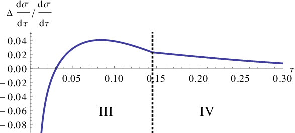

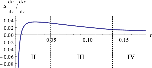
We conclude with a brief discussion of the numerical size of secondary bottom quark mass effects in the singular partonic thrust distribution at N3LL order1212 12 We use the canonical SCET counting, where N3LL order refers to matrix elements and matching conditions and four-loop renormalization group evolution. where all two-loop mass corrections were calculated from the massive gluon results via the dispersion method described above.1313 13 For the soft function the dispersion method leads to an approximate result for the two-loop non-logarithmic corrections which is however sufficient for the brief analysis carried out here. In Fig. 11a the blue solid line shows the result for the production of massless primary quarks at GeV with secondary production of the massless quarks and the bottom quark with mass GeV. The red dashed line shows the result when the bottom mass is zero. We use profile functions similar to the ones used in Ref. [29] to describe the thrust dependence of the jet and soft scale. More details are provided in Ref. [7]. The massive effects are quite sizeable. In the peak region the bottom mass leads to a reduction and in the tail region to an enhancement resulting in a reduced negative slope of the distribution. As can be seen from Fig. 11b, where the relative size of the mass effects with respect to the massless result is shown, the values of the thrust distributions are enhanced up to 4% in the dijet tail region . In the peak region the relative size of the reduction of the distribution is even larger and leads to a sizeable effect. Although non-perturbative effects have to be included for a more definite numerical analysis, it is clear that the secondary bottom mass effects are important for the analysis of event-shape distributions at lower c.m. energies from JADE [37] or from current B-factory data. In the figure we have also indicated the field theory scenarios needed to describe the respective thrust ranges according to the hierarchies of our profile functions: for GeV and GeV only scenarios III and IV can arise because for very small the bottom mass is located between the soft and the jet scale, which then increase for larger . We have implemented the factorization theorem with a strict expansion of all two-loop corrections in the product of the matching conditions and the jet and soft functions, and there is no displacement of the blue solid curve at the transition from scenario III to scenario IV. The change of slope visible at the transition point of scenarios III and IV is related to the use of the different dynamical flavor numbers for the renormalization group evolution.
An example where three scenarios are needed to describe the full thrust spectrum is the case of secondary top quark production with GeV for GeV. Here the top mass is between the hard and the jet scale for small , and also scenario II is required. The distributions with and without secondary top quark mass effects are displayed in Fig. 12a using the same labeling as in Fig. 11. We see that the behavior and the size of the secondary top quark mass corrections are very similar to the bottom quark case discussed before, albeit with the property that the peak region of the partonic distribution is confined to much smaller values due to the large c.m. energy . A more detailed numerical analysis is presented in Ref. [7].
VIII Conclusions
In this paper we have set up a method to deal with secondary massive quark radiation effects for inclusive jet cross sections. Depending on the mass value and the kinematic variables in the jet cross section, the jet invariant mass and the scale of soft large angle radiation can vary continuously crossing mass thresholds involving the secondary quark pair. This makes the theoretical method to deal with calculations of matrix elements, matching conditions and the summation of the correct large logarithmic terms complicated. We have set up an effective theory framework that combines the massless partonic modes described in soft-collinear effective theory with collinear and soft mass modes. While the collinear and soft modes for massless quarks and gluons in inclusive jets typically have different invariant masses, the mass-shell fluctuations of collinear and soft mass modes have the same invariant masses. Moreover, the mass modes can also fluctuate with invariant masses like their massless counterparts if the mass is small. This leads to different effective theories depending on the values of the mass and the kinematic variables. We have developed such an effective theory scheme for thrust in collisions considering the effects of secondary massive quark radiation (through gluon splitting) in massless quark pair production. The resulting scheme for thrust requires four different effective theories and allows for a continuous description from ultra-heavy quark masses in the decoupling limit down to the limit of vanishing quark mass where the massless description is recovered. The setup can thus be applied to every possible kinematic situation.
The mass mode setup is in the spirit of the variable flavor number scheme originally developed by Aivazis, Collins, Olness and Tung where infrared-safe hard Wilson coefficients were obtained with the subtraction of low-virtuality parton splitting terms to deal with quark masses in hadron collisions which are smaller than the hard scale but larger than . Our method represents an effective field theory realization of the variable flavor number scheme using the framework of soft-collinear effective theory for inclusive jet processes and its principles can be well applied to other processes involving heavy quark production including hadron collisions.
For thrust and other observables where the invariant mass of the massive quark pair enters the observable, it is possible to describe the secondary massive quarks through a dispersion integral involving the absorptive part of the massive quark vacuum polarization function and a massive “gluon” propagator. This allows to discuss the field theory setup for the simpler case of a spontaneously broken non-Abelian gauge theory combined with QCD involving massless quarks where the additional gauge bosons have a common mass. Conceptual as well as many technical aspects can be studied in great detail considering these massive “gluons”. In this work we have concentrated on developing the effective theory framework and the results concerning the massive gauge bosons, and we outlined the calculations required to obtain the results for secondary massive quarks. Other applications shall be addressed in subsequent work.
Acknowledgements.
We would like to thank Guido Bell and Vicent Mateu for helpful discussions and comments on the draft.References
- [1] M. Aivazis, J. C. Collins, F. I. Olness, and W.-K. Tung, Leptoproduction of heavy quarks. 2. A Unified QCD formulation of charged and neutral current processes from fixed target to collider energies, Phys. Rev. D50, 3102–3118 (1994).
- [2] M. Aivazis, F. I. Olness, and W.-K. Tung, Leptoproduction of heavy quarks. 1. General formalism and kinematics of charged current and neutral current production processes, Phys. Rev. D50, 3085–3101 (1994).
- [3] C. W. Bauer, S. Fleming, and M. E. Luke, Summing Sudakov logarithms in in effective field theory, Phys. Rev. D63, 014006 (2000).
- [4] C. W. Bauer, S. Fleming, D. Pirjol, and I. W. Stewart, An Effective field theory for collinear and soft gluons: Heavy to light decays, Phys. Rev. D63, 114020 (2001).
- [5] S. Fleming, A. H. Hoang, S. Mantry, and I. W. Stewart, Jets from massive unstable particles: Top-mass determination, Phys. Rev. D77, 074010 (2008).
- [6] S. Fleming, A. H. Hoang, S. Mantry, and I. W. Stewart, Top Jets in the Peak Region: Factorization Analysis with NLL Resummation, Phys. Rev. D77, 114003 (2008).
- [7] S. Gritschacher, A. Hoang, I. Jemos, and P. Pietrulewicz, in preparation.
- [8] I. W. Stewart, F. J. Tackmann, and W. J. Waalewijn, N-Jettiness: An Inclusive Event Shape to Veto Jets, Phys. Rev. Lett. 105, 092002 (2010).
- [9] B. A. Kniehl, M. Krawczyk, J. H. Kuhn, and R. Stuart, Hadronic Contributions to Radiative Corrections in Annihilation, Phys. Lett. B209, 337 (1988).
- [10] A. Hoang, M. Jezabek, J. H. Kuhn, and T. Teubner, Radiation of heavy quarks, Phys.Lett. B338, 330–335 (1994).
- [11] A. Hoang, J. H. Kuhn, and T. Teubner, Radiation of light fermions in heavy fermion production, Nucl. Phys. B452, 173–187 (1995).
- [12] J.-y. Chiu, F. Golf, R. Kelley, and A. V. Manohar, Electroweak Sudakov corrections using effective field theory, Phys. Rev. Lett. 100, 021802 (2008).
- [13] J.-y. Chiu, F. Golf, R. Kelley, and A. V. Manohar, Electroweak Corrections in High Energy Processes using Effective Field Theory, Phys. Rev. D77, 053004 (2008).
- [14] J.-y. Chiu, A. Fuhrer, A. H. Hoang, R. Kelley, and A. V. Manohar, Soft-Collinear Factorization and Zero-Bin Subtractions, Phys. Rev. D79, 053007 (2009).
- [15] T. Becher and M. Neubert, Drell-Yan production at small , transverse parton distributions and the collinear anomaly, Eur.Phys.J. C71, 1665 (2011).
- [16] T. Becher and G. Bell, Analytic Regularization in Soft-Collinear Effective Theory, Phys. Lett. B713, 41–46 (2012).
- [17] J.-y. Chiu, A. Jain, D. Neill, and I. Z. Rothstein, The Rapidity Renormalization Group, Phys.Rev.Lett. 108, 151601 (2012).
- [18] J.-Y. Chiu, A. Jain, D. Neill, and I. Z. Rothstein, A Formalism for the Systematic Treatment of Rapidity Logarithms in Quantum Field Theory, JHEP 1205, 084 (2012).
- [19] B. Jantzen and V. A. a. Smirnov, The Two-loop vector form-factor in the Sudakov limit, Eur. Phys. J. C47, 671–695 (2006).
- [20] S. Moch, J. Vermaseren, and A. Vogt, The Quark form-factor at higher orders, JHEP 0508, 049 (2005).
- [21] T. Becher and M. Neubert, Toward a NNLO calculation of the decay rate with a cut on photon energy. II. Two-loop result for the jet function, Phys. Lett. B637, 251–259 (2006).
- [22] A. H. Hoang and S. Kluth, Hemisphere Soft Function at O(alpha(s)**2) for Dijet Production in e+ e- Annihilation, (2008).
- [23] R. Kelley, M. D. Schwartz, R. M. Schabinger, and H. X. Zhu, The two-loop hemisphere soft function, Phys. Rev. D84, 045022 (2011).
- [24] A. Hornig, C. Lee, I. W. Stewart, J. R. Walsh, and S. Zuberi, Non-global Structure of the Dijet Soft Function, JHEP 1108, 054 (2011).
- [25] S. Moch, J. Vermaseren, and A. Vogt, The Three loop splitting functions in QCD: The Nonsinglet case, Nucl. Phys. B688, 101–134 (2004).
- [26] G. Heinrich, T. Huber, D. Kosower, and V. Smirnov, Nine-Propagator Master Integrals for Massless Three-Loop Form Factors, Phys.Lett. B678, 359–366 (2009).
- [27] R. Lee, A. Smirnov, and V. Smirnov, Analytic Results for Massless Three-Loop Form Factors, JHEP 1004, 020 (2010).
- [28] T. Becher and M. D. Schwartz, A Precise determination of from LEP thrust data using effective field theory, JHEP 0807, 034 (2008).
- [29] R. Abbate, M. Fickinger, A. H. Hoang, V. Mateu, and I. W. Stewart, Thrust at N3LL with Power Corrections and a Precision Global Fit for , Phys. Rev. D83, 074021 (2011).
- [30] A. K. Leibovich, Z. Ligeti, and M. B. Wise, Comment on quark masses in SCET, Phys. Lett. B564, 231–234 (2003).
- [31] A. Hoang, Applications of two loop calculations in the standard model and its minimal supersymmetric extension, (1995).
- [32] E. Gardi, Perturbative and nonperturbative aspects of moments of the thrust distribution in e+ e- annihilation, JHEP 0004, 030 (2000).
- [33] R. K. Ellis, D. Ross, and A. Terrano, The Perturbative Calculation of Jet Structure in Annihilation, Nucl. Phys. B178, 421 (1981).
- [34] A. V. Manohar and I. W. Stewart, The Zero-Bin and Mode Factorization in Quantum Field Theory, Phys. Rev. D76, 074002 (2007).
- [35] A. Idilbi and T. Mehen, Demonstration of the equivalence of soft and zero-bin subtractions, Phys.Rev. D76, 094015 (2007).
- [36] A. Idilbi and T. Mehen, On the equivalence of soft and zero-bin subtractions, Phys. Rev. D75, 114017 (2007).
- [37] P. Movilla Fernandez, O. Biebel, S. Bethke, S. Kluth, and P. Pfeifenschneider, A Study of event shapes and determinations of using data of annihilations at GeV to GeV, Eur. Phys. J. C1, 461–478 (1998).