During self-consistency cycles in a dft computation, recourse is made at each cycle to the Hartree energy,

Because siesta is a periodic code, in which the system and the dft mesh (typically one crystal unit cell) are replicated indefinitely in all directions, a particularly effective solution of eqn. (3) is obtained by transforming to $\textstyle k$-space using fast Fourier transforms (FFT). This method is ideal for crystals, but for finite molecular systems the dft mesh (periodic cell) must be made large enough to damp out interactions of the system with its periodic images. Physical properties may converge only slowly with the mesh size. Figure (1a,b) illustrates this for a toy model of an isolated water molecule. Although the molecule and its orbitals hold within a cube of side $5.7$ Å , a dft mesh of side 20 Å is required to achieve good convergence of the energy ($\approx-465.8$ eV) and dipole moment ($\approx 1.389$ D) in the periodic FFT computation.

We refer repeatedly to this model, using the standard double-zeta with polarisation basis set of siesta (dzp, energy shift parameter 0.02 Ry), in the local density approximation (lda, Ceperley-Alder exchange-correlation[25]). The mesh cutoff is 400 Ry. Heuristics in siesta cause the corresponding mesh step to vary slightly with the box size, in the range $0.08\pm 0.002$ Å in all calculations. The tolerances for convergence of the density matrix and energy are $10^{-6}$ and $10^{-6}$ eV respectively. Standard Troullier-Martins pseudo-potentials from the siesta library are used throughout. The model is used at the optimised geometry.

In fact, the solution of eqn. (3) for finite systems is determined uniquely by the values on a closed surface enclosing the charge density, i.e. Dirichlet boundary conditions. The dft mesh for a finite system can thus be made quite small, provided there is a recipe for accurately specifying the solution on the surface of the dft mesh.

A molecular computation thus needs; (i) an independent means of specifying the Dirichlet boundary conditions at the surface points of the finite dft mesh; (ii) an efficient solver for the boundary value problem of $V(\mathchoice{\mbox{\boldmath$\displaystyle r$}}{\mbox{\boldmath$\textstyle r$}}{\mbox{\boldmath$\scriptstyle r$}}{\mbox{\boldmath$\scriptscriptstyle r$}})$ in the interior of the domain.

Often it is desirable to assign charges to atomic centres, to be used as proxies for the full electronic density $\rho(\mathchoice{\mbox{\boldmath$\displaystyle r$}}{\mbox{\boldmath$\textstyle r$}}{\mbox{\boldmath$\scriptstyle r$}}{\mbox{\boldmath$\scriptscriptstyle r$}})$. Such schemes, e.g. Mulliken charges and ’atoms in molecules’ analysis[31], each have their own advantages and disadvantages. In classical molecular dynamics, partial atomic charges ’best fit’ to represent the Coulomb forces would be desirable. In practice, ’best fit’ representation of the Coulomb potential itself is much more tractable analytically and more common than fitting the gradient of the potential.

It long has been known[16] that matrix $\mathchoice{\mbox{\boldmath$\displaystyle A$}}{\mbox{\boldmath$\textstyle A$}}{\mbox{\boldmath$\scriptstyle A$}}{\mbox{\boldmath$\scriptscriptstyle A$}}^{\prime}$ may be ill-conditioned or singular, depending on the choice of the test points $\mathchoice{\mbox{\boldmath$\displaystyle S$}}{\mbox{\boldmath$\textstyle S$}}{\mbox{\boldmath$\scriptstyle S$}}{\mbox{\boldmath$\scriptscriptstyle S$}}_{j}$, because the far field of a set of charges is determined principally by their lowest order multipoles. In our implementation we use as $\mathchoice{\mbox{\boldmath$\displaystyle S$}}{\mbox{\boldmath$\textstyle S$}}{\mbox{\boldmath$\scriptstyle S$}}{\mbox{\boldmath$\scriptscriptstyle S$}}_{j}$’s a subset of the dft mesh points, since the full electrostatic potential is known already on the dft mesh at the end of the SCF cycles. Similar to a Connolly surface[11], the mesh points chosen are those at least at a distance $R_{\hbox{\scriptsize min}}$ from all nuclei, and at most $R_{\hbox{\scriptsize min}}+\delta R$ from some nucleus (the ’skin’ thickness $\delta R$ being in practice $\approx 0.1$ Å). Our experience with the finite support AO’s in siesta is that esp charges are physically sensible and relatively insensitive to $R_{\hbox{\scriptsize min}}$ when it is chosen from just greater than the largest AO radius, up to around $5$ Å beyond. For larger values, matrix $\mathchoice{\mbox{\boldmath$\displaystyle A$}}{\mbox{\boldmath$\textstyle A$}}{\mbox{\boldmath$\scriptstyle A$}}{\mbox{\boldmath$\scriptscriptstyle A$}}^{\prime}$ may indeed become singular. Typical mesh sizes generally lead to several thousand points within the skin, so that the main cause of any indetermination of the charges is the singularity of $\mathchoice{\mbox{\boldmath$\displaystyle A$}}{\mbox{\boldmath$\textstyle A$}}{\mbox{\boldmath$\scriptstyle A$}}{\mbox{\boldmath$\scriptscriptstyle A$}}^{\prime}$ when all the points are chosen too far away from the molecule.

We solve equation (4) using a truncated SVD algorithm, starting with $QR$ factorization of $\mathchoice{\mbox{\boldmath$\displaystyle A$}}{\mbox{\boldmath$\textstyle A$}}{\mbox{\boldmath$\scriptstyle A$}}{\mbox{\boldmath$\scriptscriptstyle A$}}^{\prime}$ as $\mathchoice{\mbox{\boldmath$\displaystyle A$}}{\mbox{\boldmath$\textstyle A$}}{\mbox{\boldmath$\scriptstyle A$}}{\mbox{\boldmath$\scriptscriptstyle A$}}^{\prime}=\mathchoice{\mbox{\boldmath$\displaystyle Q$}}{\mbox{\boldmath$\textstyle Q$}}{\mbox{\boldmath$\scriptstyle Q$}}{\mbox{\boldmath$\scriptscriptstyle Q$}}\mathchoice{\mbox{\boldmath$\displaystyle R$}}{\mbox{\boldmath$\textstyle R$}}{\mbox{\boldmath$\scriptstyle R$}}{\mbox{\boldmath$\scriptscriptstyle R$}}$, where $\textstyle Q$ is an orthogonal matrix and $\textstyle R$ is upper triangular. Singular value decomposition of $\textstyle R$ yields $\mathchoice{\mbox{\boldmath$\displaystyle R$}}{\mbox{\boldmath$\textstyle R$}}{\mbox{\boldmath$\scriptstyle R$}}{\mbox{\boldmath$\scriptscriptstyle R$}}=\mathchoice{\mbox{\boldmath$\displaystyle U$}}{\mbox{\boldmath$\textstyle U$}}{\mbox{\boldmath$\scriptstyle U$}}{\mbox{\boldmath$\scriptscriptstyle U$}}\mathchoice{\mbox{\boldmath$\displaystyle W$}}{\mbox{\boldmath$\textstyle W$}}{\mbox{\boldmath$\scriptstyle W$}}{\mbox{\boldmath$\scriptscriptstyle W$}}\mathchoice{\mbox{\boldmath$\displaystyle V$}}{\mbox{\boldmath$\textstyle V$}}{\mbox{\boldmath$\scriptstyle V$}}{\mbox{\boldmath$\scriptscriptstyle V$}}^{T}$, where $\textstyle U$ and $\textstyle V$ are orthogonal and $\textstyle W$ is diagonal (diagonal elements $w_{i}$). Small singular eigenvalues, signifying singularity of the matrix and indetermination of the $q_{i}$, are removed by setting $w_{i}=0$ if $\left|w_{i}/w_{\hbox{\scriptsize max}}\right|<\epsilon$. We standardly choose $\epsilon=10^{-9}$ . The solution, $\mathchoice{\mbox{\boldmath$\displaystyle q$}}{\mbox{\boldmath$\textstyle q$}}{\mbox{\boldmath$\scriptstyle q$}}{\mbox{\boldmath$\scriptscriptstyle q$}}^{\prime}$, of eqn. (4) is then

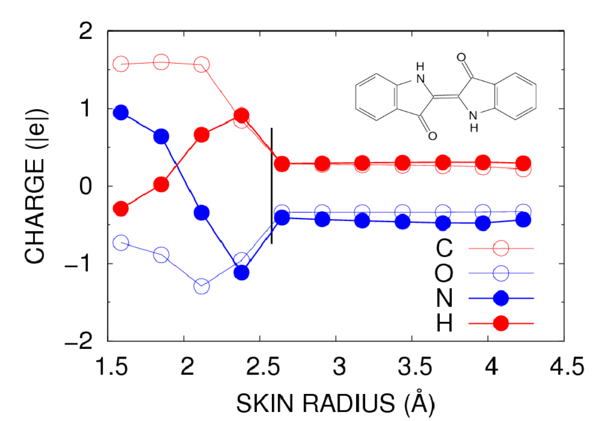
Figure (3) shows the esp charges found for polar groups in indigo, as a function of the esp shell radius $R_{\hbox{\scriptsize min}}$ ($\delta R=0.1$ Å ). Conditions are the same as for the toy water model in section 2.1. The Poisson equation was solved with the multi-grid method with Dirichlet boundary conditions from spherical harmonics up to order 4. It will be observed that the esp charges are insensitive to $R_{min}$ once the sample points are all outside the largest atomic orbital (radius $\sim 2.6$ Å). The charges on C,O,N and H are 0.28, -0.34, -0.42 and 0.29e .

It often is desirable to restrict the size of a quantum mechanical calculation to just the essential atoms for the problem at hand. Quantum mechanics/molecular mechanics (qm/mm) calculations are a prime example, as are cluster calculations in which a cluster of atoms of tractable size is cut out of a periodic material. In both cases it is necessary to correct dangling valencies left by the truncation, to reduce perturbation of the core region of the cluster. One way is to add capping atoms (usually hydrogens) to complete peripheral valencies.

Another is to turn dangling bonds into lone pairs, an approach developed by Xiao and Zhang[32] with a view to qm/mm calculations, cf. figure (4). Perturbation of the core of the cluster is then minimised by transforming the peripheral atom so capped into a ’design’ atom, with specific pseudo-potentials to mimic the electronic structure of the atom it replaces. We have extended this method to truncation on oxygen and applied it to larger systems, where we find the perturbation decays rapidly with distance from the cut bond.

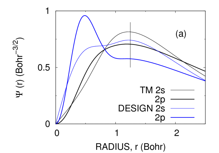
Pseudo-potentials may be produced and tested with the help of the atom program distributed with siesta. We coded ’design’ Troullier-Martins, norm conserving pseudo-potentials in atom. In the design atom approach for carbon, one adds an electron and increases the nuclear charge by one unit. But the design atom is not just nitrogen, since to minimise discrepancies between the full and the truncated molecule, it is further required that the electronic density of the design atom outside the core matches that of carbon. This constraint is achieved by rescaling the wave functions outside the core radius, per angular momentum channel, $l$, by $\eta_{l}=\left(N_{l}/N^{D}_{l}\right)^{1/2}$, where $N_{l}$ is the number of valence electrons of the original atom in shell $l$ and $N^{D}_{l}$ that in the same shell of the design atom.

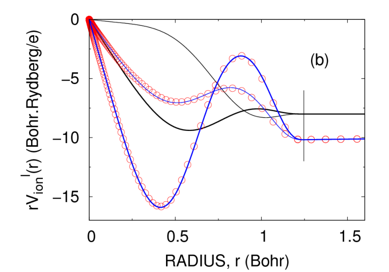
Thus, for carbon, $\eta_{\hbox{\scriptsize 2p}}=\sqrt{2/3}$, and one expects $\eta_{\hbox{\scriptsize 2s}}=1$. Compared to standard carbon, the radial 2p valence wavefunction of design carbon is therefore depressed outside the core radius, and exalted within, to accommodate the extra electron, figure (5a). In fact Xiao and Zhang adjusted $\eta_{\hbox{\scriptsize 2s}}$, optimising it with respect to the geometrical parameters of their target molecules, yielding in their case $\eta_{\hbox{\scriptsize 2s}}=0.91$. Our implementation closely follows ref. [32], and indeed our design carbon pseudo-potentials agree very closely with those of Xiao and Zhang, see figure (5b).

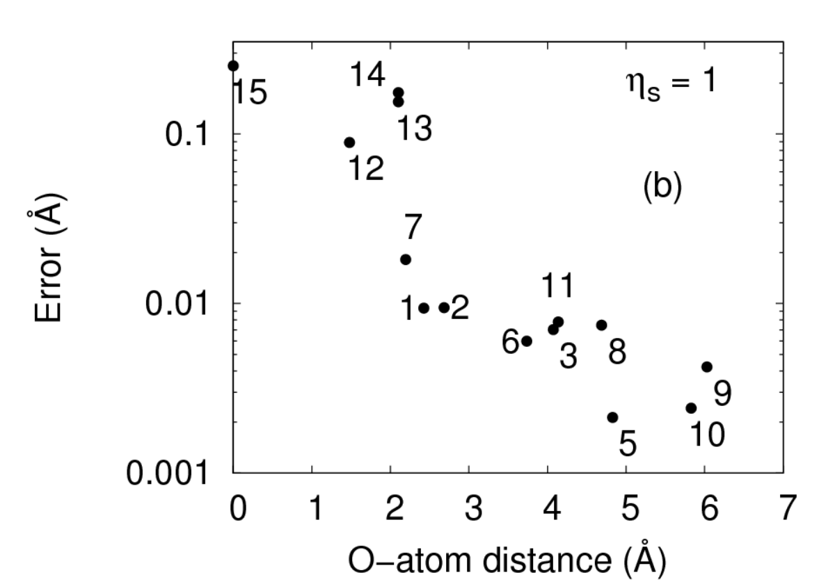
We extended the design atom approach to truncation on oxygen. In this case, $\eta_{\hbox{\scriptsize 2p}}=\sqrt{4/5}\sim 0.89$. We varied $\eta_{\hbox{\scriptsize 2s}}$ in a series of truncations on the oxygen atom of the toy benzyl carbamate in figure (6a), similar in structure to graftable photosensitizers of reactive oxygen species of interest to us[22]. Here, we show results for $\eta_{\hbox{\scriptsize 2s}}=1$; reducing it deteriorated the results. Figure (6b) compares the geometries of the full and the truncated forms, both fully optimised (lda, standard dzp basis). The important part of the molecule is the phenyl ring, standing in for the chromophore. Our measure of quality is therefore to bring three phenyl carbons (atoms 4,1 and 3 in fig. 6a), of both the full and the truncated molecules, respectively to the origin, on to the $Ox$ axis and into the $Oxy$ plane, and to compute the distances between corresponding atoms, shown in fig. (6b) as a scatter plot of error vs. distance to the oxygen atom before truncation. It will be observed that the error of placement of atoms in the fragment relative to the full molecule, drops off fast as a function of the distance from the design oxygen, being under 10^-2 Å for those in the ring. Complete $Z$-matrices are provided in the supplementary information.