Exact sum rules for inhomogeneous drums

Paolo Amore Email: paolo.amore@gmail.com Address: Facultad de Ciencias, CUICBAS, Universidad de Colima,
Bernal Díaz del Castillo 340, Colima, Colima, Mexico

Abstract

We derive general expressions for the sum rules of the eigenvalues of drums of arbitrary shape and arbitrary density, obeying different boundary conditions. The formulas that we present are a generalization of the analogous formulas for one dimensional inhomogeneous systems that we have obtained in a previous paper. We also discuss the extension of these formulas to higher dimensions. We show that in the special case of a density depending only on one variable the sum rules of any integer order can be expressed in terms of a single series. As an application of our result we derive exact sum rules for the a homogeneous circular annulus with different boundary conditions, for a homogeneous circular sector and for a radially inhomogeneous circular annulus with Dirichlet boundary conditions.

Keywords:

Helmholtz equation; inhomogeneous drum; sum rules

1 Introduction

This paper considers the problem of obtaining explicit expressions for the sum rules

\displaystyle Z(p)=\sum_{n}\frac{1}{E_{n}^{p}}\ \ ,\ \ p=2,3,\dots

(1)

where $E_{n}$ are the eigenvalues of the Helmholtz equation

\displaystyle(-\Delta)\psi_{n}(x,y)=E_{n}\Sigma(x,y)\psi_{n}(x,y)\ .

(2)

over a two dimensional domain $(x,y)\in\Omega$ . We assume that $\Omega$ is a domain where a orthonormal basis is known (square, circle, etc) since the more general problem on an arbitrary domain may be reduced to the form of eq.(2) using a conformal map. Here $n$ is the set of quantum numbers which fully specifies a solution and $\Sigma(x,y)$ may either be a physical density, a density obtained from a conformal map or a composition of the two.

Unfortunately, the evaluation of $Z(p)$ using eq.(1) requires the knowledge of the eigenvalues of the problem, which is granted only in special cases. In a recent paper, ref.[1], we have discussed an alternative approach which uses the representation of $Z(p)$ directly as the trace of the hermitian operator

\displaystyle\hat{Q}^{p}\equiv\left(\sqrt{\Sigma}(-\Delta)^{-1}\sqrt{\Sigma}\right)^{p}

(3)

where $p>1$ is a real exponent. We have proved there that the eigenvalues of $\hat{Q}$ are the reciprocals of the eigenvalues of eq.(2) and therefore the trace of $\hat{Q}^{p}$ provides the spectral zeta function associated with the problem of eq.(2). For integer values of $p$ it is possible to obtain explicit expressions for the trace $\hat{Q}^{p}$ and therefore for $Z(p)$ : we have discussed specific examples in ref. [1]. In the general case of non integer values of $p$ , we have shown in ref.[1] that it is possible to evaluate the trace using perturbation theory; although the expressions obtained following this approach are defined for $p>1$ (in $d$ dimensions, $p>d/2$ ) it is possible to perform their analytic continuation to $s<1$ : in this way we have obtained the Casimir energy of specific systems in one, two and three dimensions.

There is a large number of works where spectral sum rules for given sytems have been studied: these include the sum rules for quantum mechanical anharmonic oscillators [2, 3], for potentials $V(r)=gr^{p}$ ( $p>0$ , $g>0$ ) [4], for Aharonov-Bohm quantum billiards [5, 6], for the zeroes of Bessel functions [4, 7], for the Selberg’s zeta function for compact Riemann surfaces [8] (see also [9]), for quantum mechanical one dimensional potentials[10], for two dimensional domains close to the unit disk [11], for the cardioid and related domains[12], for a $\mathcal{PT}$ -symmetric hamiltonian [13, 14].

In this paper we provide a method to calculate the sum rules for the eigenvalues of the negative laplacian in two and higher dimensions, for systems of arbitrary density. The approach that we describe is based on the results of ref. [1], which are now expressed in terms of the appropriate Green’s functions and used to derive a general formula for the sum rule of arbitrary order $p>d/2$ ( $d$ are the dimensions of the problem). This formula is a generalization of the analogous formula for one-dimensional inhomogeneous systems obtained in ref. [15], where it has been applied to a number of examples (in the case of a particular inhomogeneous string we have been able to obtain sum rules up to order nine). In two dimensions the reference domain chosen for our calculation is a rectangle (for $d>2$ we use its generalization), although it can be any domain where a Green’s function is available. In particular in two dimensions, our formula should be compared with the equivalent formula obtained by Itzykson, Moussa and Luck [16], who expressed the sum rule of a given order $n$ for the Dirichlet eigenvalues of the negative laplacian on an arbitrary domain $T$ in terms of the Green’s function on the upper half plane; moreover Dittmar [17] has obtained a formula for the sum rule of order two for the eigenvalues of the negative laplacian on a two dimensional domain both for Dirichlet and Neumann boundary conditions in terms of the Green’s functions on a circle (see Theorems 2.1 and 3.3 of ref. [17]). The expressions that we derive in this paper apply to sum rules of arbitrary order, to different boundary conditions an both to homogenous and inhomogeneous systems.

The paper is organized as follows: in Section 2 we derive the expressions for the Green’s functions on a rectangle of sides $a$ and $b$ , with different boundary conditions; in Section 3 we obtain a general formula for the sum rules of arbitrary order in two dimensions; in Section 4 we discuss the generalization of this formula to higher dimensions; in Section 5 we consider some applications of our formula; finally, in Section 6 we draw our conclusions.

2 Green’s functions on a rectangle

In this section we derive explicit expressions for the Green’s functions of the negative laplacian on a rectangle of sides $a$ and $b$ and obeying different boundary conditions at the borders. We consider the cases of Dirichlet, Neumann and periodic bc on the borders of the rectangle, of mixed bc, Dirichlet-Neumann, Dirichlet-periodic, Neumann-periodic and mixed Neumann-Dirichlet boundary condition in one direction and periodic in the other direction.

2.1 Dirichlet boundary conditions

We consider the rectangular region $(-a/2,a/2)\times(-b/2,b/2)$ and assume Dirichlet boundary conditions at the border of this region; the Green’s function for the negative laplacian is

\displaystyle G^{(D)}(x,y;x^{\prime},y^{\prime})

\displaystyle=

\displaystyle\sum_{n_{x}=1}^{\infty}\sum_{n_{y}=1}^{\infty}\frac{\psi^{(D)}_{n_{x}}(x)\phi^{(D)}_{n_{y}}(y)\psi^{(D)}_{n_{x}}(x^{\prime})\phi^{(D)}_{n_{y}}(y^{\prime})}{\epsilon^{(D)}_{n_{x}}+\eta^{(D)}_{n_{y}}}\ .

(4)

Here $\psi_{n_{x}}(x)$ and $\phi_{n_{y}}(y)$ are the Dirichlet eigenfunction of the 1D negative laplacian on $x\in(-a/2,a/2)$ and $y\in(-b/2,b/2)$ respectively:

	$\displaystyle\psi_{n_{x}}(x)\equiv\sqrt{\frac{2}{a}}\ \sin\left(\frac{n_{x}\pi}{a}(x+a/2)\right)\ \ ,\ \ n_{x}$	$\displaystyle=$	$\displaystyle 1,2,\dots$		(5)
	$\displaystyle\psi_{n_{y}}(y)\equiv\sqrt{\frac{2}{b}}\ \sin\left(\frac{n_{y}\pi}{b}(y+b/2)\right)\ \ ,\ \ n_{y}$	$\displaystyle=$	$\displaystyle 1,2,\dots$		(6)

$\epsilon^{(D)}_{n_{x}}$ and $\eta^{(D)}_{n_{y}}$ are the Dirichlet eigenvalues of the 1D negative laplacian in the two directions:

\displaystyle\epsilon^{(D)}_{n_{x}}=\frac{n_{x}^{2}\pi^{2}}{a^{2}}\ \ \ ,\ \ \ \eta^{(D)}_{n_{y}}=\frac{n_{y}^{2}\pi^{2}}{b^{2}}\ .

(7)

Eq.(4) may be cast in the form:

\displaystyle G^{(D)}(x,y;x^{\prime},y^{\prime})

\displaystyle=

\displaystyle\sum_{n_{x}=1}^{\infty}g_{n_{x}}^{(D)}(y,y^{\prime})\psi^{(D)}_{n_{x}}(x)\psi^{(D)}_{n_{x}}(x^{\prime})\ ,

(8)

where (see Eq.(3.169) and problem 2.15 of Ref. [18]):

	$\displaystyle g_{n_{x}}^{(D)}(y,y^{\prime})$	$\displaystyle\equiv$	$\displaystyle\sum_{n_{y}=1}^{\infty}\frac{\phi^{(D)}_{n_{y}}(y)\phi^{(D)}_{n_{y}}(y^{\prime})}{\epsilon^{(D)}_{n_{x}}+\eta^{(D)}_{n_{y}}}$		(9)
		$\displaystyle=$	$\displaystyle\frac{\sinh\left(\sqrt{\epsilon_{n_{x}}^{(D)}}(y_{<}+b/2)\right)\sinh\left(\sqrt{\epsilon_{n_{x}}^{(D)}}(b/2-y_{>})\right)}{\sqrt{\epsilon_{n_{x}}^{(D)}}\sinh\sqrt{\epsilon_{n_{x}}^{(D)}}b}\ .$		(9)

We have introduced the notation $y_{<}\equiv\min(y,y^{\prime})$ and $y_{>}\equiv\max(y,y^{\prime})$ .

We also define

	$\displaystyle G^{(D)}(x,y;x^{\prime},y^{\prime})$	$\displaystyle\equiv$	$\displaystyle G_{+}^{(D)}(x,y;x^{\prime},y^{\prime})\theta(y-y^{\prime})$		(10)
		$\displaystyle+$	$\displaystyle G_{-}^{(D)}(x,y;x^{\prime},y^{\prime})\theta(y^{\prime}-y)\ ,$		(10)

where the explicit form of $G_{\pm}^{(D)}(x,y;x^{\prime},y^{\prime})$ is easily obtained from Eq. (8).

Notice also that

	$\displaystyle G_{+}^{(D)}(x,y;x^{\prime},y^{\prime})$	$\displaystyle=$	$\displaystyle G_{-}^{(D)}(x,-y;x^{\prime},-y^{\prime})$
	$\displaystyle G_{+}^{(D)}(x,y^{\prime};x^{\prime},y)$	$\displaystyle=$	$\displaystyle G_{-}^{(D)}(x,y;x^{\prime},y^{\prime})\ .$

It is also possible to express Eq.(8) in an alternative form, observing that

\displaystyle\frac{1}{\sinh\frac{\pi nb}{a}}=2\sum_{j=0}^{\infty}e^{-(2j+1)\pi nb/a}

(11)

Upon substitution of this expansion inside Eq.(8) we have

$\displaystyle G^{(D)}(x,y;x^{\prime},y^{\prime})$	$\displaystyle\equiv$	$\displaystyle\sum_{j=0}^{\infty}G_{j}^{(D)}(x,y;x^{\prime},y^{\prime})$	(12)
	$\displaystyle=$	$\displaystyle\frac{1}{4\pi}\sum_{j=0}^{\infty}\log\frac{\Omega_{j}(x_{-},x_{+},y_{-},y_{+})}{\Theta_{j}(x_{-},x_{+},y_{-},y_{+})}$
	$\displaystyle=$	$\displaystyle\frac{1}{4\pi}\log\prod_{j=0}^{\infty}\frac{\Omega_{j}(x_{-},x_{+},y_{-},y_{+})}{\Theta_{j}(x_{-},x_{+},y_{-},y_{+})}\ ,$

where

$\displaystyle\Omega_{j}(x_{-},x_{+},y_{-},y_{+})$	$\displaystyle\equiv$	$\displaystyle\left(\cosh\left(\frac{\pi(2bj+b-y_{+})}{a}\right)-\cos\left(\frac{\pi x_{-}}{a}\right)\right)$	(13)
	$\displaystyle\cdot$	$\displaystyle\left(\cosh\left(\frac{\pi(2bj+b+y_{+})}{a}\right)-\cos\left(\frac{\pi x_{-}}{a}\right)\right)$
	$\displaystyle\cdot$	$\displaystyle\left(\cosh\left(\frac{\pi(2b(j+1)-\|y_{-}\|)}{a}\right)+\cos\left(\frac{\pi x_{+}}{a}\right)\right)$
	$\displaystyle\cdot$	$\displaystyle\left(\cosh\left(\frac{\pi(\|y_{-}\|+2bj)}{a}\right)+\cos\left(\frac{\pi x_{+}}{a}\right)\right)$
$\displaystyle\Theta_{j}(x_{-},x_{+},y_{-},y_{+})$	$\displaystyle\equiv$	$\displaystyle\left(\cosh\left(\frac{\pi(2bj+b-y_{+})}{a}\right)+\cos\left(\frac{\pi x_{+}}{a}\right)\right)$	(14)
	$\displaystyle\cdot$	$\displaystyle\left(\cosh\left(\frac{\pi(2bj+b+y_{+})}{a}\right)+\cos\left(\frac{\pi x_{+}}{a}\right)\right)$
	$\displaystyle\cdot$	$\displaystyle\left(\cosh\left(\frac{\pi(2b(j+1)-\|y_{-}\|)}{a}\right)-\cos\left(\frac{\pi x_{-}}{a}\right)\right)$
	$\displaystyle\cdot$	$\displaystyle\left(\cosh\left(\frac{\pi(\|y_{-}\|+2bj)}{a}\right)-\cos\left(\frac{\pi x_{-}}{a}\right)\right)$

and $x_{\pm}\equiv x_{1}\pm x_{2}$ , $y_{\pm}\equiv y_{1}\pm y_{2}$ .

Notice that

\displaystyle\Theta_{0}(0,x_{+},0,y_{+})=0

and therefore $G^{(D)}(x,y;x^{\prime},y^{\prime})$ diverges logarithmically when $x_{2}\rightarrow x_{1}$ and $y_{2}\rightarrow y_{1}$ .

Although the series in Eq.(12) converges more rapidly than the series in Eq.(8), in general the latter is more appropriate for the evaluation of the sum rules.

2.2 Neumann boundary conditions

We now come to the calculation of the Green’s function for Neumann boundary conditions ¹¹ 1 We have not found references reporting the equivalent expressions of eq. (9) for boundary conditions other than Dirichlet. The results that we report for these cases have been derived in the present paper following the same approach used for eq. (9).; in this case we have

\displaystyle G^{(N)}(x,y;x^{\prime},y^{\prime})

\displaystyle=

\displaystyle\sum^{\prime}_{n_{x},u_{x},n_{y},u_{y}}\frac{\psi^{(N)}_{n_{x},u_{x}}(x)\phi^{(N)}_{n_{y},u_{y}}(y)\psi^{(N)}_{n_{x},u_{x}}(x^{\prime})\phi^{(N)}_{n_{y},u_{y}}(y^{\prime})}{\epsilon^{(N)}_{n_{x},u_{x}}+\eta^{(N)}_{n_{y},u_{y}}}\ ,

(15)

where $\sum^{\prime}_{n_{x},u_{x},n_{y},u_{y}}$ is the sum over all possible values of the quantum number, with the exclusion of the divergent term corresponding to $n_{x}=n_{y}=0$ and $u_{x}=u_{y}=1$ ²² 2 $\sum^{\prime}_{n_{x},u_{x},n_{y},u_{y}}c_{n_{x},u_{x},n_{y},u_{y}}\equiv\sum_{n_{x}=1}^{\infty}\sum_{u_{x}=1}^{2}c_{n_{x},u_{x},0,1}+\sum_{n_{y}=1}^{\infty}\sum_{u_{y}=1}^{2}c_{0,1,n_{y},u_{y}}+\sum_{n_{x}=1}^{\infty}\sum_{u_{x}=1}^{2}\sum_{n_{y}=1}^{\infty}\sum_{u_{y}=1}^{2}c_{n_{x},u_{x},n_{y},u_{y}}$ .

Here $\epsilon_{n_{x},u_{x}}^{(N)}$ and $\eta_{n_{y},u_{y}}^{(N)}$ are the Neumann eigenvalues of the negative laplacian in the two orthogonal directions;

	$\displaystyle\epsilon_{n_{x},u_{x}}^{(N)}$	$\displaystyle=$	$\displaystyle\left\{\begin{array}[]{ccccc}\frac{4n_{x}^{2}\pi^{2}}{a^{2}}&,&u_{x}=1&,&n_{x}=0,1,2,\dots\\ \frac{(2n_{x}-1)^{2}\pi^{2}}{a^{2}}&,&u_{x}=2&,&n_{x}=1,2,\dots\\ \end{array}\right.$
	$\displaystyle\eta_{n_{y},u_{y}}^{(N)}$	$\displaystyle=$	$\displaystyle\left\{\begin{array}[]{ccccc}\frac{4n_{y}^{2}\pi^{2}}{b^{2}}&,&u_{y}=1&,&n_{y}=0,1,2,\dots\\ \frac{(2n_{y}-1)^{2}\pi^{2}}{b^{2}}&,&u_{y}=2&,&n_{y}=1,2,\dots\\ \end{array}\right.$

and $\psi_{n_{x},u_{x}}^{(N)}(x)$ and $\phi_{n_{y},u_{y}}^{(N)}(y)$ are its eigenfunctions:

	$\displaystyle\psi_{n_{x},u_{x}}^{(N)}(x)$	$\displaystyle=$	$\displaystyle\left\{\begin{array}[]{ccc}\sqrt{\frac{1}{a}}&,&n_{x}=0\ ,\ u_{x}=1\\ \sqrt{\frac{2}{a}}\cos\frac{2n_{x}\pi x}{a}&,&n_{x}>0\ ,\ u_{x}=1\\ \sqrt{\frac{2}{a}}\sin\frac{(2n_{x}-1)\pi x}{a}&,&n_{x}\geq 0\ ,\ u_{x}=2\\ \end{array}\right.$
	$\displaystyle\phi_{n_{y},u_{y}}^{(N)}(y)$	$\displaystyle=$	$\displaystyle\left\{\begin{array}[]{ccc}\sqrt{\frac{1}{b}}&,&n_{y}=0\ ,\ u_{y}=1\\ \sqrt{\frac{2}{b}}\cos\frac{2n_{y}\pi y}{b}&,&n_{y}>0\ ,\ u_{y}=1\\ \sqrt{\frac{2}{b}}\sin\frac{(2n_{y}-1)\pi y}{b}&,&n_{y}\geq 0\ ,\ u_{y}=2\\ \end{array}\right.$

In this case Eq. (15) may be expressed as

	$\displaystyle G^{(N)}(x,y;x^{\prime},y^{\prime})$	$\displaystyle=$	$\displaystyle\frac{1}{a}g_{0,1}^{(N)}(y,y^{\prime})$		(30)
		$\displaystyle+$	$\displaystyle\sum_{n_{x}=1}^{\infty}\sum_{u_{x}=1}^{2}g_{n_{x},u_{x}}^{(N)}(y,y^{\prime})\psi^{(N)}_{n_{x},u_{x}}(x)\psi^{(N)}_{n_{x},u_{x}}(x^{\prime})$		(30)

where $g_{n_{x},u_{x}}^{(N)}(y,y^{\prime})$ is the analogous of Eq.(9) for Neumann boundary conditions:

\displaystyle g_{n_{x},u_{x}}^{(N)}(y,y^{\prime})

\displaystyle\equiv

\displaystyle\frac{1-\delta_{n_{x},0}}{b\epsilon^{(N)}_{n_{x},u_{x}}}+\sum_{u_{y}=1}^{2}\sum_{n_{y}=1}^{\infty}\frac{\phi^{(N)}_{n_{y},u_{y}}(y)\phi^{(N)}_{n_{y},u_{y}}(y^{\prime})}{\epsilon^{(N)}_{n_{x},u_{x}}+\eta^{(N)}_{n_{y},u_{y}}}.

For $n_{x}=0$ and $u_{x}=1$ , $g_{n_{x},u_{x}}^{(N)}(y,y^{\prime})$ reduces to the one-dimensional Green’s function with Neumann boundary conditions, which is reported in Ref. [15]:

\displaystyle g_{0,1}^{(N)}(y,y^{\prime})

\displaystyle=

\displaystyle\frac{b^{2}+6b(y_{<}-y_{>})+6\left(y_{>}^{2}+y_{<}^{2}\right)}{12b}\ .

(31)

For $n_{x}>0$ and $u_{x}=1,2$ we have

\displaystyle g_{n_{x},u_{x}}^{(N)}(y,y^{\prime})

\displaystyle=

\displaystyle\frac{\cosh\left(\sqrt{\eta^{(N)}_{n_{x},u_{x}}}\frac{(b-2y_{>})}{2}\right)\cosh\left(\sqrt{\eta^{(N)}_{n_{x},u_{x}}}\frac{(b+2y_{<})}{2}\right)}{\sqrt{\eta^{(N)}_{n_{x},u_{x}}}\sinh\left(\sqrt{\eta^{(N)}_{n_{x},u_{x}}}b\right)}\ .

(32)

2.3 Dirichlet-Neumann boundary conditions

We now come to the calculation of the Green’s function for mixed Dirichlet-Neumann boundary conditions; in this case we have

\displaystyle G^{(DN)}(x,y;x^{\prime},y^{\prime})

\displaystyle=

\displaystyle\sum_{n_{x},n_{y},u_{y}}\frac{\psi^{(D)}_{n_{x}}(x)\phi^{(N)}_{n_{y},u_{y}}(y)\psi^{(D)}_{n_{x}}(x^{\prime})\phi^{(N)}_{n_{y},u_{y}}(y^{\prime})}{\epsilon^{(D)}_{n_{x}}+\eta^{(N)}_{n_{y},u_{y}}}\ ,

(33)

where

\displaystyle\sum_{n_{x},n_{y},u_{y}}c_{n_{x},n_{y},u_{y}}=\sum_{n_{x}=1}^{\infty}c_{n_{x},0,1}+\sum_{n_{x}=1}^{\infty}\sum_{n_{y}=1}^{\infty}\sum_{u_{y}=1}^{2}c_{n_{x},n_{y},u_{y}}\ .

(34)

We may express eq.(33) as:

\displaystyle G^{(DN)}(x,y;x^{\prime},y^{\prime})

\displaystyle=

\displaystyle\frac{g_{0,1}^{(DN)}(x,x^{\prime})}{b}+\sum_{n_{y}=1}^{\infty}\sum_{u_{y}=1}^{2}g_{n_{y},u_{y}}^{(DN)}(x,x^{\prime})\phi^{(N)}_{n_{y},u_{y}}(y)\phi^{(N)}_{n_{y},u_{y}}(y^{\prime})

(35)

where

\displaystyle g_{n_{y},u_{y}}^{(DN)}(x,x^{\prime})

\displaystyle\equiv

\displaystyle\sum_{n_{x}=1}^{\infty}\frac{\psi^{(D)}_{n_{x}}(x)\psi^{(D)}_{n_{x}}(x^{\prime})}{\epsilon^{(D)}_{n_{x}}+\eta^{(N)}_{n_{y},u_{y}}}

(36)

For $n_{y}=0$ and $u_{y}=1$ $g_{n_{y},u_{y}}^{(DN)}(x,x^{\prime})$ is the 1D Green’s function for Dirichlet bc reported in Ref.[15]:

\displaystyle g_{0,1}^{(DN)}(x,x^{\prime})

\displaystyle=

\displaystyle\frac{(a-2x_{>})(a+2x_{<})}{4a}

(37)

while for $n_{y}>0$ and $u_{y}=1,2$

\displaystyle g_{n_{y},u_{y}}^{(DN)}(x,x^{\prime})

\displaystyle=

\displaystyle\frac{\sinh\left(\sqrt{\eta^{(N)}_{n_{y},u_{y}}}(x_{>}-\frac{a}{2})\right)\sinh\left(\sqrt{\eta^{(N)}_{n_{y},u_{y}}}(\frac{a}{2}+x_{<})\right)}{\sqrt{\eta^{(N)}_{n_{y},u_{y}}}\ \sinh\left(\sqrt{\eta^{(N)}_{n_{y},u_{y}}}\ a\right)}

(38)

for $n_{y}>0$ and $u_{y}=1,2$ .

Alternatively we may write the Green’s function as

\displaystyle G^{(DN)}(x,y;x^{\prime},y^{\prime})

\displaystyle=

\displaystyle\sum_{n_{x}=1}^{\infty}\tilde{g}_{n_{x}}^{(DN)}(y,y^{\prime})\psi^{(D)}_{n_{x}}(x)\psi^{(D)}_{n_{x}}(x^{\prime})

(39)

where

	$\displaystyle\tilde{g}_{n_{x}}^{(DN)}(y,y^{\prime})$	$\displaystyle\equiv$	$\displaystyle\frac{1}{b\ \epsilon^{(D)}_{n_{x}}}+\sum_{u_{y}=1}^{2}\sum_{n_{y}=1}^{\infty}\frac{\phi^{(N)}_{n_{y},u_{y}}(y)\phi^{(N)}_{n_{y},u_{y}}(y^{\prime})}{\epsilon^{(D)}_{n_{x}}+\eta^{(N)}_{n_{y},u_{y}}}$		(40)
		$\displaystyle=$	$\displaystyle\frac{\cosh\left(\sqrt{\epsilon_{n_{x}}^{(D)}}(b/2-y_{>})\right)\cosh\left(\sqrt{\epsilon_{n_{x}}^{(D)}}(b/2+y_{<})\right)}{\sqrt{\epsilon_{n_{x}}^{(D)}}\ \sinh(b\sqrt{\epsilon_{n_{x}}^{(D)}})}$		(40)

2.4 Periodic boundary conditions

We now come to the calculation of the Green’s function for periodic boundary conditions; in this case we have

\displaystyle G^{(P)}(x,y;x^{\prime},y^{\prime})

\displaystyle=

\displaystyle\sum_{n_{x},u_{x},n_{y},u_{y}}^{\prime}\frac{\psi^{(P)}_{n_{x},u_{x}}(x)\phi^{(P)}_{n_{y},u_{y}}(y)\psi^{(P)}_{n_{x},u_{x}}(x^{\prime})\phi^{(P)}_{n_{y},u_{y}}(y^{\prime})}{\epsilon^{(P)}_{n_{x},u_{x}}+\eta^{(P)}_{n_{y},u_{y}}}\ ,

(41)

where we have excluded from the sum the divergent term corresponding to $n_{x}=n_{y}=0$ and $u_{x}=u_{y}=1$ as for the case of Neumann bc.

Here $\epsilon_{n_{x},u_{x}}^{(P)}$ and $\eta_{n_{y},u_{y}}^{(P)}$ are the Neumann eigenvalues of the negative laplacian in the two orthogonal directions;

\displaystyle\epsilon_{n_{x},u_{x}}^{(P)}=\frac{4\pi^{2}n_{x}^{2}}{a^{2}}\ \ \ ,\ \ \ \eta_{n_{y},u_{y}}^{(N)}=\frac{4\pi^{2}n_{y}^{2}}{b^{2}}

(42)

and $\psi_{n_{x},u_{x}}^{(P)}(x)$ and $\phi_{n_{y},u_{y}}^{(P)}(y)$ are its eigenfunctions:

	$\displaystyle\psi_{n_{x},u_{x}}^{(P)}(x)$	$\displaystyle=$	$\displaystyle\left\{\begin{array}[]{ccc}\sqrt{\frac{1}{a}}&,&n_{x}=0\ ,\ u_{x}=1\\ \sqrt{\frac{2}{a}}\cos\frac{2n_{x}\pi x}{a}&,&n_{x}>0\ ,\ u_{x}=1\\ \sqrt{\frac{2}{a}}\sin\frac{2n_{x}\pi x}{a}&,&n_{x}\geq 0\ ,\ u_{x}=2\\ \end{array}\right.$
	$\displaystyle\phi_{n_{y},u_{y}}^{(P)}(y)$	$\displaystyle=$	$\displaystyle\left\{\begin{array}[]{ccc}\sqrt{\frac{1}{b}}&,&n_{y}=0\ ,\ u_{y}=1\\ \sqrt{\frac{2}{b}}\cos\frac{2n_{y}\pi y}{b}&,&n_{y}>0\ ,\ u_{y}=1\\ \sqrt{\frac{2}{b}}\sin\frac{2n_{y}\pi y}{b}&,&n_{y}\geq 0\ ,\ u_{y}=2\\ \end{array}\right.$

In this case Eq. (41) may be expressed as

\displaystyle G^{(P)}(x,y;x^{\prime},y^{\prime})

\displaystyle=

\displaystyle\frac{g_{0,1}^{(P)}(y,y^{\prime})}{a}+\sum_{n_{x}=1}^{\infty}\sum_{u_{x}=1}^{2}g_{n_{x},u_{x}}^{(P)}(y,y^{\prime})\psi^{(P)}_{n_{x},u_{x}}(x)\psi^{(P)}_{n_{x},u_{x}}(x^{\prime})

(51)

where

\displaystyle g_{n_{x},u_{x}}^{(P)}(y,y^{\prime})

\displaystyle\equiv

\displaystyle\frac{1-\delta_{n_{x},0}}{b\ \epsilon^{(P)}_{n_{x},u_{x}}}+\sum_{u_{y}=1}^{2}\sum_{n_{y}=1}^{\infty}\frac{\phi^{(P)}_{n_{y},u_{y}}(y)\phi^{(P)}_{n_{y},u_{y}}(y^{\prime})}{\epsilon^{(P)}_{n_{x},u_{x}}+\eta^{(P)}_{n_{y},u_{y}}}.

For $n_{x}=0$ and $u_{x}=1$ , $g_{n_{x},u_{x}}^{(P)}(y,y^{\prime})$ reduces to the one-dimensional Green’s function with periodic boundary conditions reported in ref. [15]:

\displaystyle g_{0,1}^{(P)}(y,y^{\prime})

\displaystyle=

\displaystyle\frac{b^{2}-6b|y-y^{\prime}|+6\left(y-y^{\prime}\right)^{2}}{12b}\ .

(52)

For $n_{x}>0$ and $u_{x}=1,2$ we have

\displaystyle g_{n_{x},u_{x}}^{(P)}(y,y^{\prime})

\displaystyle=

\displaystyle\frac{\cosh\left(\sqrt{\epsilon_{n_{x},u_{x}}^{(P)}}(|y-y^{\prime}|-b/2)\right)}{2\sqrt{\epsilon_{n_{x},u_{x}}^{(P)}}\sinh\left(\frac{b\sqrt{\epsilon_{n_{x},u_{x}}^{(P)}}}{2}\right)}

(53)

2.5 Dirichlet-Periodic boundary conditions

We now come to the calculation of the Green’s function for mixed Dirichlet-periodic boundary conditions; in this case we have

\displaystyle G^{(DP)}(x,y;x^{\prime},y^{\prime})

\displaystyle=

\displaystyle\sum_{n_{x},n_{y},u_{y}}\frac{\psi^{(D)}_{n_{x}}(x)\phi^{(P)}_{n_{y},u_{y}}(y)\psi^{(D)}_{n_{x}}(x^{\prime})\phi^{(P)}_{n_{y},u_{y}}(y^{\prime})}{\epsilon^{(D)}_{n_{x}}+\eta^{(P)}_{n_{y},u_{y}}}\ .

(54)

where $\sum_{n_{x},n_{y},u_{y}}$ is defined in eq.(34).

We may express this Green’s functions as

	$\displaystyle G^{(DP)}(x,y;x^{\prime},y^{\prime})$	$\displaystyle=$	$\displaystyle\frac{g_{0,1}^{(DP)}(x,x^{\prime})}{b}$		(55)
		$\displaystyle+$	$\displaystyle\sum_{n_{y}=1}^{\infty}\sum_{u_{y}=1}^{2}g_{n_{y},u_{y}}^{(DP)}(x,x^{\prime})\phi^{(P)}_{n_{y},u_{y}}(y)\phi^{(P)}_{n_{y},u_{y}}(y^{\prime})$		(55)

where

\displaystyle g_{n_{y},u_{y}}^{(DP)}(x,x^{\prime})

\displaystyle\equiv

\displaystyle\sum_{n_{x}=1}^{\infty}\frac{\psi^{(D)}_{n_{x}}(x)\psi^{(D)}_{n_{x}}(x^{\prime})}{\epsilon^{(D)}_{n_{x}}+\eta^{(P)}_{n_{y},u_{y}}}

(56)

For $n_{y}=0$ and $u_{y}=1$ , $g_{n_{y},u_{y}}^{(DP)}(x,x^{\prime})$ reduces to the 1D Green’s function for Dirichlet bc:

\displaystyle g_{0,1}^{(DP)}(x,x^{\prime})

\displaystyle=

\displaystyle\frac{(a-2x_{>})(a+2x_{<})}{4a}

(57)

For $n_{y}>0$ and $u_{y}=1,2$

\displaystyle g_{n_{y},u_{y}}^{(DP)}(x,x^{\prime})

\displaystyle=

\displaystyle\frac{\sinh\left(\sqrt{\eta^{(P)}_{n_{y},u_{y}}}(x_{>}-\frac{a}{2})\right)\sinh\left(\sqrt{\eta^{(P)}_{n_{y},u_{y}}}(\frac{a}{2}+x_{<})\right)}{\sqrt{\eta^{(P)}_{n_{y},u_{y}}}\ \sinh\left(\sqrt{\eta^{(P)}_{n_{y},u_{y}}}\ a\right)}

(58)

Alternatively we may write the Green’s function as

\displaystyle G^{(DP)}(x,y;x^{\prime},y^{\prime})

\displaystyle=

\displaystyle\sum_{n_{x}=1}^{\infty}\tilde{g}_{n_{x}}^{(DP)}(y,y^{\prime})\psi^{(D)}_{n_{x}}(x)\psi^{(D)}_{n_{x}}(x^{\prime})

(59)

where

	$\displaystyle\tilde{g}_{n_{x}}^{(DP)}(y,y^{\prime})$	$\displaystyle\equiv$	$\displaystyle\frac{1}{b\ \epsilon^{(D)}_{n_{x}}}+\sum_{u_{y}=1}^{2}\sum_{n_{y}=1}^{\infty}\frac{\phi^{(P)}_{n_{y},u_{y}}(y)\phi^{(P)}_{n_{y},u_{y}}(y^{\prime})}{\epsilon^{(D)}_{n_{x}}+\eta^{(P)}_{n_{y},u_{y}}}$		(60)
		$\displaystyle=$	$\displaystyle\frac{\cosh\left(\sqrt{\epsilon_{n_{x}}^{(D)}}(\|y-y^{\prime}\|-b/2)\right)}{2\sqrt{\epsilon_{n_{x}}^{(D)}}\sinh\left(\frac{b\sqrt{\epsilon_{n_{x}}^{(D)}}}{2}\right)}$		(60)

2.6 Neumann-Periodic boundary conditions

We now come to the calculation of the Green’s function for mixed Neumann-periodic boundary conditions:

\displaystyle G^{(NP)}(x,y;x^{\prime},y^{\prime})

\displaystyle=

\displaystyle\sum_{n_{x},u_{x},n_{y},u_{y}}^{\prime}\frac{\psi^{(N)}_{n_{x},u_{x}}(x)\phi^{(P)}_{n_{y},u_{y}}(y)\psi^{(N)}_{n_{x},u_{x}}(x^{\prime})\phi^{(P)}_{n_{y},u_{y}}(y^{\prime})}{\epsilon^{(N)}_{n_{x},u_{x}}+\eta^{(P)}_{n_{y},u_{y}}}\ .

(61)

where $\sum_{n_{x},u_{x},n_{y},u_{y}}^{\prime}$ has been defined earlier for the case of Neumann boundary conditions.

We may express the Green’s functions as

\displaystyle G^{(NP)}(x,y;x^{\prime},y^{\prime})

\displaystyle=

\displaystyle\frac{g_{01}^{(NP)}(x,x^{\prime})}{b}+\sum_{n_{y}=1}^{\infty}\sum_{u_{y}=1}^{2}g_{n_{y},u_{y}}^{(NP)}(x,x^{\prime})\phi^{(P)}_{n_{y},u_{y}}(y)\phi^{(P)}_{n_{y},u_{y}}(y^{\prime})

(62)

where

\displaystyle g_{n_{y},u_{y}}^{(NP)}(x,x^{\prime})

\displaystyle\equiv

\displaystyle\frac{1-\delta_{n_{y},0}}{a\ \eta^{(P)}_{n_{y},u_{y}}}+\sum_{n_{x}=1}^{\infty}\sum_{u_{x}=1}^{2}\frac{\psi^{(N)}_{n_{x},u_{x}}(x)\psi^{(N)}_{n_{x},u_{x}}(x^{\prime})}{\epsilon^{(N)}_{n_{x},u_{x}}+\eta^{(P)}_{n_{y},u_{y}}}\ .

(63)

For $n_{y}=0$ and $u_{y}=1$ , $g_{n_{y},u_{y}}^{(NP)}(x,x^{\prime})$ reduces to the 1D Green’s function for Neumann bc reported in Ref. [15]

\displaystyle g_{0,1}^{(NP)}(x,x^{\prime})

\displaystyle=

\displaystyle\frac{a^{2}-6a|x-x^{\prime}|+6(x^{2}+{x^{\prime}}^{2})}{12a}\ .

(64)

For $n_{y}>0$ and $u_{y}=1,2$

\displaystyle g_{n_{y},u_{y}}^{(NP)}(x,x^{\prime})

\displaystyle=

\displaystyle\frac{\cosh\left(\sqrt{\eta^{(P)}_{n_{y},u_{y}}}\frac{(a-2x_{>})}{2}\right)\cosh\left(\sqrt{\eta^{(P)}_{n_{y},u_{y}}}\frac{(a+2x_{<})}{2}\right)}{\sqrt{\eta^{(P)}_{n_{y},u_{y}}}\sinh\left(\sqrt{\eta^{(P)}_{n_{y},u_{y}}}a\right)}\ .

(65)

Alternatively we may write the Green’s function as

\displaystyle G^{(NP)}(x,y;x^{\prime},y^{\prime})

\displaystyle=

\displaystyle\frac{\tilde{g}_{01}^{(NP)}(y,y^{\prime})}{a}+\sum_{n_{x}=1}^{\infty}\sum_{u_{x}=1}^{2}\tilde{g}_{n_{x},u_{x}}^{(NP)}(y,y^{\prime})\psi^{(N)}_{n_{x},u_{x}}(x)\psi^{(N)}_{n_{x},u_{x}}(x^{\prime})

(66)

where

\displaystyle\tilde{g}_{n_{x},u_{x}}^{(NP)}(y,y^{\prime})

\displaystyle\equiv

\displaystyle\frac{1-\delta_{n_{x},0}}{b\ \epsilon^{(N)}_{n_{x},u_{x}}}+\sum_{u_{y}=1}^{2}\sum_{n_{y}=0}^{\infty}\frac{\phi^{(P)}_{n_{y},u_{y}}(y)\phi^{(P)}_{n_{y},u_{y}}(y^{\prime})}{\epsilon^{(N)}_{n_{x},u_{x}}+\eta^{(P)}_{n_{y},u_{y}}}\ .

(67)

For $n_{y}=0$ and $u_{y}=1$ , $\tilde{g}_{n_{y},u_{y}}^{(NP)}(x,x^{\prime})$ reduces to the 1D Green’s function for periodic bc reported in Ref. [15]

\displaystyle g_{0,1}^{(NP)}(y,y^{\prime})

\displaystyle=

\displaystyle\frac{b^{2}-6b|y-y^{\prime}|+6\left(y-y^{\prime}\right)^{2}}{12b}\ .

(68)

For $n_{y}>0$ and $u_{y}=1,2$

\displaystyle\tilde{g}_{n_{x},u_{x}}^{(NP)}(y,y^{\prime})

\displaystyle=

\displaystyle\frac{\cosh\left(\sqrt{\epsilon_{n_{x},u_{x}}^{(N)}}(|y-y^{\prime}|-b/2)\right)}{2\sqrt{\epsilon_{n_{x},u_{x}}^{(N)}}\sinh\left(\frac{b\sqrt{\epsilon_{n_{x},u_{x}}^{(N)}}}{2}\right)}\ .

2.7 Neumann-Dirichlet-Periodic boundary conditions

We now come to the calculation of the Green’s function for mixed Neumann-Dirichlet-periodic boundary conditions: in this case we assume Neumann bc at $x=-a/2$ , Dirichlet bc at $x=+a/2$ and periodic boundary conditions at $y=\pm b/2$ .

We have

\displaystyle G^{(NDP)}(x,y;x^{\prime},y^{\prime})

\displaystyle=

\displaystyle\sum_{n_{x},n_{y},u_{y}}\frac{\psi^{(ND)}_{n_{x}}(x)\phi^{(P)}_{n_{y},u_{y}}(y)\psi^{(ND)}_{n_{x}}(x^{\prime})\phi^{(P)}_{n_{y},u_{y}}(y^{\prime})}{\epsilon^{(ND)}_{n_{x}}+\eta^{(P)}_{n_{y},u_{y}}}

(69)

where $\sum_{n_{x},n_{y},u_{y}}$ is defined in eq.(34).

We have

\displaystyle\psi_{n_{x}}^{(ND)}(x)=\sqrt{\frac{2}{a}}\sin\left(\frac{\pi(2n_{x}-1)(3a+2x)}{4a}\right)

(70)

and

\displaystyle\epsilon^{(ND)}_{n_{x}}=\frac{(2n_{x}-1)^{2}\pi^{2}}{4a^{2}}

(71)

We may cast the Green’s function of Eq.(69) as

\displaystyle G^{(NDP)}(x,y;x^{\prime},y^{\prime})

\displaystyle=

\displaystyle\frac{g_{0,1}^{(NDP)}(x,x^{\prime})}{b}+\sum_{n_{y}=1}^{\infty}\sum_{u_{y}=1}^{2}g_{n_{y},u_{y}}^{(NDP)}(x,x^{\prime})\phi^{(P)}_{n_{y},u_{y}}(y))\phi^{(P)}_{n_{y},u_{y}}(y^{\prime})

(72)

where

\displaystyle g_{n_{y},u_{y}}^{(NDP)}(x,x^{\prime})

\displaystyle\equiv

\displaystyle\sum_{n_{x}=1}^{\infty}\frac{\psi^{(ND)}_{n_{x}}(x)\psi^{(ND)}_{n_{x}}(x^{\prime})}{\epsilon^{(ND)}_{n_{x}}+\eta^{(P)}_{n_{y},u_{y}}}\ .

(73)

For $n_{y}=0$ and $u_{y}=1$ we have the one-dimensional Green’s function for mixed Neumann-Dirichlet boundary conditions:

\displaystyle g_{0,1}^{(NDP)}(x,x^{\prime})

\displaystyle=

\displaystyle(-x_{>}+a/2)

(74)

For $n_{y}>0$ and $u_{y}=1,2$ we have

\displaystyle g_{n_{y},u_{y}}^{(NDP)}(x,x^{\prime})

\displaystyle=

\displaystyle\frac{{\rm sech}\left(a\sqrt{\epsilon_{n_{y},u_{y}}^{(P)}}\right)\sinh\left(\frac{1}{2}\sqrt{\epsilon_{n_{y},u_{y}}^{(P)}}(a-2x_{>})\right)\cosh\left(\frac{1}{2}\sqrt{\epsilon_{n_{y},u_{y}}^{(P)}}(a+2x_{<})\right)}{\sqrt{\epsilon_{n_{y},u_{y}}^{(P)}}}

(75)

Alternatively we may cast the Green’s function of Eq.(69) as

\displaystyle G^{(NDP)}(x,y;x^{\prime},y^{\prime})

\displaystyle=

\displaystyle\sum_{n_{x}=1}^{\infty}\tilde{g}_{n_{x}}^{(NDP)}(y,y^{\prime})\psi^{(ND)}_{n_{x}}(x))\psi^{(ND)}_{n_{x}}(x^{\prime})

(76)

where

	$\displaystyle\tilde{g}_{n_{x}}^{(NDP)}(y,y^{\prime})$	$\displaystyle\equiv$	$\displaystyle\frac{1}{b\ \epsilon^{(ND)}_{n_{x}}}+\sum_{n_{y}=1}^{\infty}\sum_{u_{y}=1}^{2}\frac{\phi^{(P)}_{n_{y}u_{y}}(y)\phi^{(P)}_{n_{y}u_{y}}(y^{\prime})}{\epsilon^{(ND)}_{n_{x}}+\eta^{(P)}_{n_{y},u_{y}}}$		(77)
		$\displaystyle=$	$\displaystyle\frac{\cosh\left(\sqrt{\epsilon_{n_{x}}^{(ND)}}(\|y-y^{\prime}\|-b/2)\right)}{2\sqrt{\epsilon_{n_{x}}^{(ND)}}\sinh\left(\frac{b\sqrt{\epsilon_{n_{x}}^{(ND)}}}{2}\right)}$		(77)

2.8 Dirichlet-Neumann-Periodic boundary conditions

In this case we assume Dirichlet bc at $x=-a/2$ , Neumann bc at $x=+a/2$ and periodic boundary conditions at $y=\pm b/2$ . This case is trivial since the basis with

\displaystyle\psi_{n_{x}}^{(DN)}(x)=\psi_{n_{x}}^{(ND)}(-x)

(78)

Therefore

\displaystyle g_{n_{y},u_{y}}^{(DNP)}(x,x^{\prime})

\displaystyle=

\displaystyle g_{n_{y},u_{y}}^{(NDP)}(-x,-x^{\prime})

(79)

3 Exact sum rules

In Ref. [15] we have derived a set of rules which allow one to obtain explicit expressions for the sum rules for the eigenvalues of an inhomogeneous string:

\displaystyle Z_{n}=\sum_{p}\frac{1}{E_{p}^{n}}\ ,

(80)

with $n=1,2,\dots$ .

These rules may be easily generalized to higher dimensions: in particular in two dimensions the sum rule of order $n$ may be expressed as

	$\displaystyle Z^{(D)}_{n}$	$\displaystyle=$	$\displaystyle\int d^{2}R_{1}\int d^{2}R_{2}\dots\int d^{2}R_{n}\ G({\bf R}_{n};{\bf R}_{1})$		(81)
		$\displaystyle\cdot$	$\displaystyle\prod_{i=1}^{n-1}\left[G({\bf R}_{i};{\bf R}_{i+1})\right]\prod_{i=1}^{n}\left[\Sigma({\bf R}_{i})\right]$		(81)

where ${\bf R}_{i}\equiv(x_{i},y_{i})$ and $|x_{i}|\leq a/2$ , $|y_{i}|\leq b/2$ . Here $G({\bf R}_{i};{\bf R}_{j})$ is the 2D Green’s function obeying the appropriate bc and $\Sigma({\bf R}_{i})$ is a density ³³ 3 Notice that $G({\bf R},{\bf R}^{\prime})$ is the Green’s function on any domain where a basis is known, such as a rectangle or a circle..

As done in Ref. [15] it is convenient to cast this expression in an alternative form, using the "y-ordered" Green’s function:

	$\displaystyle Z^{(D)}_{n}$	$\displaystyle=$	$\displaystyle\int_{-a/2}^{a/2}dx_{1}\int_{-a/2}^{a/2}dx_{2}\dots\int_{-a/2}^{a/2}dx_{n}\int_{-b/2}^{b/2}dy_{1}\ \int_{-b/2}^{y_{1}}dy_{2}\dots\int_{-b/2}^{y_{n-1}}dy_{n}$		(82)
		$\displaystyle\cdot$	$\displaystyle\mathcal{G}\left({\bf R}_{1},{\bf R}_{2},\dots,{\bf R}_{n}\right)\prod_{i=1}^{n}\left[\Sigma({\bf R}_{i})\right]\ ,$		(82)

where

\displaystyle\mathcal{G}\left({\bf R}_{1},{\bf R}_{2},\dots,{\bf R}_{n}\right)\equiv\left\{G({\bf R}_{n};{\bf R}_{1})\prod_{i=1}^{n-1}\left[G({\bf R}_{i};{\bf R}_{i+1})\right]\right\}_{\mathcal{P}}

(83)

and

\displaystyle\left\{f({\bf R}_{1},\dots,{\bf R}_{n})\right\}_{\mathcal{P}}\equiv\sum_{\rm permutations}f({\bf R}_{p_{1}},\dots,{\bf R}_{p_{n}})\ .

(84)

For example, the expressions for $\mathcal{G}$ up to order $4$ are:

$\displaystyle\mathcal{G}\left({\bf R}_{1}\right)$	$\displaystyle=$	$\displaystyle G_{+}(x_{1},y_{1};x_{1},y_{1})$
$\displaystyle\mathcal{G}\left({\bf R}_{1},{\bf R}_{2}\right)$	$\displaystyle=$	$\displaystyle 2\ \left[G_{+}(x_{1},y_{1};x_{2},y_{2})\right]^{2}$
$\displaystyle\mathcal{G}\left({\bf R}_{1},{\bf R}_{2},{\bf R}_{3}\right)$	$\displaystyle=$	$\displaystyle 6\ G_{+}(x_{1},y_{1};x_{2},y_{2})G_{+}(x_{2},y_{2};x_{3},y_{3})G_{+}(x_{1},y_{1};x_{3},y_{3})$
$\displaystyle\mathcal{G}\left({\bf R}_{1},{\bf R}_{2},{\bf R}_{3},{\bf R}_{4}\right)$	$\displaystyle=$	$\displaystyle 8\left[G_{+}(x_{1},y_{1};x_{2},y_{2})G_{+}(x_{1},y_{1};x_{4},y_{4})G_{+}(x_{2},y_{2};x_{3},y_{3})G_{+}(x_{3},y_{3};x_{4},y_{4})\right.$
	$\displaystyle+$	$\displaystyle\left.G_{+}(x_{1},y_{1};x_{3},y_{3})G_{+}(x_{1},y_{1};x_{4},y_{4})G_{+}(x_{2},y_{2};x_{3},y_{3})G_{+}(x_{2},y_{2};x_{4},y_{4})\right.$
	$\displaystyle+$	$\displaystyle\left.G_{+}(x_{1},y_{1};x_{2},y_{2})G_{+}(x_{1},y_{1};x_{3},y_{3})G_{+}(x_{2},y_{2};x_{4},y_{4})G_{+}(x_{3},y_{3};x_{4},y_{4})\right]$

We can therefore calculate $Z(n)$ with the diagrammatic rules:

1.

Draw n points ${\bf R}_{1},\dots,{\bf R}_{n}$ on a line;
2.

Connect each point to any two other points in all possible inequivalent ways excluding the disconnected diagrams and the diagrams corresponding to a cyclic permutation of the points;
3.

Associate a density $\Sigma({\bf R}_{i})$ at each point ${\bf R}_{i}$ ( $i=1,\dots,n$ );
4.

Associate a factor $G_{+}({\bf R}_{i};{\bf R}_{j})$ to each line connecting ${\bf R}_{i}$ to ${\bf R}_{j}$ ( $i<j$ );
5.

Multiply the result by a factor $2n$ , corresponding to the $n$ cyclic permutations of each inequivalent configuration and to the 2 possible directions in which each diagram can be traveled;

Integrate the expression obtained from the steps above over the internal points:

\displaystyle\int_{-a/2}^{a/2}dx_{1}\int_{-a/2}^{a/2}dx_{2}\dots\int_{-a/2}^{a/2}dx_{n}\int_{-b/2}^{b/2}dy_{1}\ \int_{-b/2}^{y_{1}}dy_{2}\dots\int_{-b/2}^{y_{n-1}}dy_{n}

It is easy to convince oneself that for the sum rule of order $n$ there are $n!/2n=(n-1)!/2$ independent diagrams (for $n>2$ ).

These rules imply that the sum rule of order $n$ for a general density contains $n$ series, one for each factor $G_{+}({\bf R}_{i};{\bf R}_{j})$ appearing in the expression; however, in the case of a density which depends only on one variable the orthogonality of the eigenfunctions along the homogeneous direction allow to reduce the multiple series to a single series, leaving only the integrals along the direction where the density varies.

Assuming for simplicity that $\Sigma=\Sigma(y)$ , and expressing for the Green’s function as

\displaystyle G_{+}(x,y;x^{\prime},y^{\prime})

\displaystyle=

\displaystyle\sum_{p}^{\infty}g_{p}^{(+)}(y,y^{\prime})\psi_{p}(x)\psi_{p}(x^{\prime})

(85)

we obtain:

\displaystyle Z^{(D)}_{n}

\displaystyle=

\displaystyle\sum_{p}\int_{-b/2}^{b/2}dy_{1}\ \int_{-b/2}^{y_{1}}dy_{2}\dots\int_{-b/2}^{y_{n-1}}dy_{n}\ \mathcal{Q}\left(y_{1},y_{2},\dots,y_{n}\right)\prod_{i=1}^{n}\left[\Sigma(y_{i})\right]\ ,

(86)

where

\displaystyle\mathcal{Q}\left(y_{1},y_{2},\dots,y_{n}\right)\equiv\left\{g_{p}(y_{n};y_{1})\prod_{i=1}^{n-1}\left[g_{p}(y_{i};y_{i+1})\right]\right\}_{\mathcal{P}}\ .

(87)

4 Higher dimensions

We briefly discuss how these results generalize to the case of $d>2$ dimensions; we consider a $d$ -dimensional region with $|x_{i}|\leq a_{i}/2$ and $i=1,\dots,d$ . For simplicity we restrict our analysis to Dirichlet boundary conditions, since the cases corresponding to the other boundary conditions can be obtained in an analogous way.

The Green’s function reads

	$\displaystyle G^{(D)}(x_{1},\dots,x_{d};x^{\prime}_{1},\dots,x^{\prime}_{d})$	$\displaystyle=$	$\displaystyle\sum_{n_{1}=1}^{\infty}\dots\sum_{n_{d}=1}^{\infty}\frac{1}{\epsilon^{(1D)}_{n_{1}}+\dots+\epsilon^{(dD)}_{n_{d}}}$		(88)
		$\displaystyle\cdot$	$\displaystyle\psi^{(1D)}_{n_{1}}(x_{1})\dots\psi^{(dD)}_{n_{d}}(x_{d})\psi^{(1D)}_{n_{1}}(x^{\prime}_{1})\dots\psi^{(dD)}_{n_{d}}(x^{\prime}_{d})$		(88)

where:

\displaystyle\psi^{(iD)}_{n_{i}}(x_{i})\equiv\sqrt{\frac{2}{a_{i}}}\ \sin\left(\frac{n_{i}\pi}{a_{i}}(x_{i}+a_{i}/2)\right)\ \ ,\ \ n_{i}

\displaystyle=

\displaystyle 1,2,\dots

and

\displaystyle\epsilon^{(iD)}_{n_{i}}\equiv\frac{n_{i}^{2}\pi^{2}}{a_{i}^{2}}\ \ ,\ \ n_{i}

\displaystyle=

\displaystyle 1,2,\dots\ .

(89)

We may now apply Eq.(9) on any of the $d$ series contained in Eq.(88); for instance, if we use it on the $d^{th}$ series we have

	$\displaystyle G^{(D)}(x_{1},\dots,x_{d};x^{\prime}_{1},\dots,x^{\prime}_{d})$	$\displaystyle=$	$\displaystyle\sum_{n_{1}=1}^{\infty}\dots\sum_{n_{d-1}=1}^{\infty}g_{n_{1},\dots,n_{d-1}}^{(D)}(x_{d},x^{\prime}_{d})$		(90)
		$\displaystyle\cdot$	$\displaystyle\psi^{(1D)}_{n_{1}}(x_{1})\dots\psi^{(d-1\ D)}_{n_{d-1}}(x_{d-1})\psi^{(1D)}_{n_{1}}(x^{\prime}_{1})\dots\psi^{(d-1\ D)}_{n_{d-1}}(x^{\prime}_{d-1})$		(90)

where

	$\displaystyle g_{n_{1},\dots,n_{d-1}}^{(D)}(x_{d},x^{\prime}_{d})$	$\displaystyle\equiv$	$\displaystyle\sum_{n_{d}=1}^{\infty}\frac{\psi^{(dD)}_{n_{d}}(x_{d})\psi^{(dD)}_{n_{d}}(x^{\prime}_{d})}{\epsilon^{(dD)}_{n_{d}}+\Gamma_{n_{1},\dots,n_{d-1}}}$		(91)
		$\displaystyle=$	$\displaystyle\frac{\sinh\left(\sqrt{\Gamma_{n_{1},\dots,n_{d-1}}}(x_{d<}+a_{d}/2)\right)\sinh\left(\sqrt{\Gamma_{n_{1},\dots,n_{d-1}}}(a_{d}/2-x_{d>})\right)}{\sqrt{\Gamma_{n_{1},\dots,n_{d-1}}}\sinh\sqrt{\Gamma_{n_{1},\dots,n_{d-1}}}a_{d}}$		(91)

and

\displaystyle\Gamma_{n_{1},\dots,n_{d-1}}\equiv\sum_{i=1}^{d-1}\epsilon^{(iD)}_{ni}\ .

(92)

The expressions for the sum rules in this case are the analogous of the ones discussed in the previous section, with the appropriate Green’s functions and density, which is now a function of $d$ variables.

It is interesting to see what happens in the case of a density which depends only on one direction, for instance $\Sigma=\Sigma(x_{d})$ . In this case, as for the two dimensional case, the eigenfunctions corresponding to the homogeneous directions can be eliminated from the expressions for the sum rules, using their orthogonality. Therefore the sum rules of any integer order for a d-dimensional system of this kind can be expressed in term of $d-1$ infinite series.

5 Applications

We now discuss few applications of the results obtained in the previous sections.

5.1 Circular annulus

In Refs.[1, 19] we have discussed the application of perturbation theory to the study of the spectrum of a circular annulus. In particular, in ref. [1] we have evaluated the sum rule of order two for the eigenvalues of the circular annulus of unit external radius and internal radius $r$ , using the matrix elements of the conformal density and we have calculated the Casimir energy of the annulus in the limit $r\rightarrow 1^{-}$ .

We will now apply the results of the previous sections to obtain explicit expressions for the sum rules for a circular annulus: the function

\displaystyle f(z)=e^{z+\frac{1}{2}\log r_{min}}

(93)

maps the rectangle $\left[\frac{1}{2}\log r_{min},-\frac{1}{2}\log r_{min}\right]\times\left[-\pi,\pi\right]$ onto a circular annulus of external radius $R=1$ and internal radius $r_{min}$ . Instead of solving the Helmholtz equation on the annulus, using the conformal map we may solve an equivalent Helmholtz equation for an inhomogeneous medium of density

\displaystyle\Sigma(x,y)=r_{min}\ e^{2x}

(94)

over the rectangle [1, 19, 22]. Since this density depends only on one coordinate, we will be able to obtain general expressions for the sum rules of the circular annulus in terms of a single series, as we have pointed out in the previous section.

Refer to caption — Figure 1: Circular annulus obtained acting with the map (93) the rectangle $\left[\frac{1}{2}\log r_{min},-\frac{1}{2}\log r_{min}\right]\times\left[-\pi,\pi\right]$ . Periodic boundary conditions are imposed on the dashed line.

We will discuss the two cases of an annulus with either Dirichlet or Neumann bc at the border: the first case corresponds to using Dirichlet bc along the $x$ direction and periodic bc along the $y$ direction; the second case corresponds to using Neumann bc along the $x$ direction and periodic bc along the $y$ direction. Notice that using Dirichlet bc along the $y$ direction would correspond to studying an annulus with a transverse cut [1].

Applying the general formulas derived in this paper it is possible to obtain explicit expressions for the sum rules of the circular annulus; for example the sum rule of order two is obtained as

	$\displaystyle Z^{(DP)}_{2}(r_{min})$	$\displaystyle=$	$\displaystyle 2\int_{\log r_{min}}^{-\log r_{min}}dx\ \int_{\log r_{min}}^{x}dx^{\prime}\left[g_{0,1}^{(DP)}(x,x^{\prime})\right]^{2}\Sigma(x)\Sigma(x^{\prime})$
		$\displaystyle+$	$\displaystyle 2\sum_{n_{y}=1}^{\infty}\sum_{u_{y}=1}^{2}\int_{\log r_{min}}^{-\log r_{min}}dx\ \int_{\log r_{min}}^{x}dx^{\prime}\left[g_{n_{y},u_{y}}^{(DP)}(x,x^{\prime})\right]^{2}\Sigma(x)\Sigma(x^{\prime})$

Using the explicit expression for $g_{0,1}^{(DP)}(x,x^{\prime})$ and performing the integrations one obtains

$\displaystyle Z^{(DP)}_{2}(r_{min})$	$\displaystyle=$	$\displaystyle\frac{r_{min}^{4}\log^{4}(r_{min})}{4-4r_{min}^{4}}-\frac{5}{64}\left(r_{min}^{4}-1\right)\log^{2}(r_{min})+\frac{1}{16}\left(r_{min}^{2}-1\right)^{2}\log(r_{min})$	(95)
	$\displaystyle+$	$\displaystyle\frac{r_{min}^{4}\log^{5}(r_{min})}{2\left(r_{min}^{2}-1\right)^{2}}-\frac{\log^{3}(r_{min})}{144\left(r_{min}^{2}+1\right)^{2}}\left(26r^{8}+73r_{min}^{6}+62r_{min}^{4}\right.$
	$\displaystyle+$	$\displaystyle\left.73r_{min}^{2}-3\pi^{2}\left(r_{min}^{2}+1\right)^{2}\left(r_{min}^{4}+1\right)+26\right)$
	$\displaystyle+$	$\displaystyle\sum_{n=3}^{\infty}\left[\frac{n\left(n^{2}+5\right)\left(r_{min}^{4}-1\right)r_{min}^{4n}}{8\left(n^{2}-4\right)\left(n^{2}-1\right)^{2}\left(r_{min}^{2n}-1\right)^{2}}+\frac{n^{2}\left(r_{min}^{2}-1\right)^{2}r_{min}^{2n}}{2\left(n^{2}-1\right)^{2}\left(r_{min}^{2n}-1\right)^{2}}\right]$

This expression may be cast in terms of a more rapidly convergent series observing that $0<r_{min}<1$ and expanding the factor $1/\left(r_{min}^{2n}-1\right)^{2}$ in powers of $r$ . After performing the summation over $n$ one is left with the new series:

$\displaystyle Z^{(DP)}_{2}(r_{min})$	$\displaystyle=$	$\displaystyle-\frac{\left(r_{min}^{4}-1\right)^{2}\left(r_{min}^{4}+1\right){\rm Li}_{2}\left(r_{min}^{4}\right)}{16r_{min}^{4}}+\frac{\left(r_{min}^{2}-1\right)^{2}\left(r_{min}^{4}+1\right){\rm Li}_{2}\left(r_{min}^{2}\right)}{8r_{min}^{2}}$	(96)
	$\displaystyle+$	$\displaystyle\frac{r^{4}\log(r_{min})}{4\left(1-r_{min}^{4}\right)}-\frac{5\left(r_{min}^{4}-1\right)}{64\log(r_{min})}+\frac{\left(r_{min}^{2}-1\right)^{2}}{16\log^{2}(r_{min})}$
	$\displaystyle-$	$\displaystyle\frac{\left(r_{min}^{2}-1\right)^{3}\left(r_{min}^{2}+1\right)\log\left(1-r_{min}^{2}\right)}{8r_{min}^{2}}$
	$\displaystyle-$	$\displaystyle\frac{\left(r_{min}^{4}-1\right)^{3}\left(r_{min}^{8}+r_{min}^{4}+1\right)\log\left(1-r_{min}^{4}\right)}{16r_{min}^{8}}+\frac{r_{min}^{4}\log^{2}(r_{min})}{2\left(r_{min}^{2}-1\right)^{2}}$
	$\displaystyle+$	$\displaystyle\frac{1}{576}\left[71r_{min}^{12}-202r_{min}^{8}+274r_{min}^{6}-297r_{min}^{4}+12\pi^{2}\left(r_{min}^{4}+1\right)\right.$
	$\displaystyle+$	$\displaystyle\left.\frac{36}{r_{min}^{4}}-66r_{min}^{2}+\frac{4\left(5r_{min}^{4}-54r_{min}^{2}-27\right)}{\left(r_{min}^{2}+1\right)^{2}}\right]$
	$\displaystyle+$	$\displaystyle\sum_{j=1}^{\infty}(j+1)\left[\frac{1}{16}\left(r_{min}^{4}-1\right)\left(r_{min}^{4j}-1\right)r_{min}^{-2j}{\rm Li}_{2}\left(r_{min}^{2j}\right)\right.$
	$\displaystyle-$	$\displaystyle\left.\frac{1}{16}\left(r_{min}^{4}-1\right)\left(r_{min}^{4j+8}-1\right)r_{min}^{-2(j+2)}{\rm Li}_{2}\left(r_{min}^{2j+4}\right)\right.$
	$\displaystyle+$	$\displaystyle\left.\frac{1}{8}\left(r_{min}^{2}-1\right)^{2}\left(r_{min}^{4j+4}+1\right)r_{min}^{-2(j+1)}{\rm Li}_{2}\left(r_{min}^{2j+2}\right)\right.$
	$\displaystyle+$	$\displaystyle\left.\frac{1}{16}\left(r_{min}^{4}-1\right)\left(r_{min}^{2j}-1\right)^{2}\left(r_{min}^{2j}+r_{min}^{4j}+1\right)r_{min}^{-4j}\log\left(1-r_{min}^{2j}\right)\right.$
	$\displaystyle-$	$\displaystyle\left.\frac{1}{16}\left(r_{min}^{4}-1\right)\left(r_{min}^{2j+4}-1\right)^{2}\left(r_{min}^{2j+4}+r_{min}^{4j+8}+1\right)r_{min}^{-4(j+2)}\log\left(1-r_{min}^{2j+4}\right)\right.$
	$\displaystyle-$	$\displaystyle\left.\frac{1}{8}\left(r_{min}^{2}-1\right)^{2}\left(r_{min}^{4j+4}-1\right)r_{min}^{-2(j+1)}\log\left(1-r_{min}^{2j+2}\right)\right.$
	$\displaystyle+$	$\displaystyle\left.\frac{r^{-2(j+2)}}{576}\left(-3\left(r_{min}^{2}-1\right)^{2}\left(r_{min}^{4}-4r_{min}^{2}+1\right)r_{min}^{4j+4}\right.\right.$
	$\displaystyle+$	$\displaystyle\left.\left.\left(r_{min}^{2}-1\right)^{2}\left(71r_{min}^{8}+142r_{min}^{6}+14r_{min}^{4}+142r_{min}^{2}+71\right)r_{min}^{6j+4}\right.\right.$
	$\displaystyle+$	$\displaystyle\left.\left.36\left(r_{min}^{4}-1\right)^{2}\right)\right]$

Clearly the rate of convergence of this series increases for $r_{min}\rightarrow 0^{+}$ : in this limit one obtains the behavior

	$\displaystyle Z^{(DP)}_{2}(r_{min})$	$\displaystyle\approx$	$\displaystyle\left(\frac{\pi^{2}}{48}-\frac{5}{32}\right)+\left(\frac{1}{16\log^{2}(r_{min})}+\frac{5}{64\log(r_{min})}\right)$		(97)
		$\displaystyle-$	$\displaystyle r_{min}^{2}\left(\frac{1}{8\log^{2}(r_{min})}+\frac{7}{48}\right)+\dots$		(97)

Notice that

\displaystyle\lim_{r_{min}\rightarrow 0^{+}}Z^{(DP)}_{2}(r_{min})=\left(\frac{\pi^{2}}{48}-\frac{5}{32}\right)\approx 0.04936675836

(98)

is the Dirichlet sum rule of order two for the unit circle.

Notice also that the derivative of $Z^{(DP)}_{2}(r_{min})$ diverges at $r=0$ :

\displaystyle\lim_{r_{min}\rightarrow 0^{+}}\frac{dZ^{(DP)}_{2}(r_{min})}{dr_{min}}=-\frac{1}{8r_{min}\log^{3}(r_{min})}-\frac{5}{64r_{min}\log^{2}(r_{min})}=-\infty

(99)

In a similar way we may obtain the sum rule of higher orders: although we have proved that these sum rules will involve a single series, since the density depends only on one direction, their expressions become lengthier and we do not see any advantage in reporting them here.

Instead, we investigate explicitly the limit of an infinitesimal hole, as done in the previous case:

$\displaystyle Z^{(DP)}_{3}(r_{min})$	$\displaystyle\approx$	$\displaystyle\left(\frac{\zeta(3)}{32}+\frac{35}{768}-\frac{\pi^{2}}{128}\right)$	(100)
	$\displaystyle+$	$\displaystyle\left(\frac{1}{64\log^{3}(r_{min})}+\frac{15}{512\log^{2}(r_{min})}+\frac{23}{1152\log(r_{min})}\right)$
	$\displaystyle-$	$\displaystyle r_{min}^{2}\left(\frac{3}{64\log^{3}(r_{min})}+\frac{15}{512\log^{2}(r_{min})}+\frac{19}{1536}\right)+\dots$

Notice that

\displaystyle\lim_{r_{min}\rightarrow 0^{+}}Z^{(DP)}_{3}(r_{min})=\frac{\zeta(3)}{32}+\frac{35}{768}-\frac{\pi^{2}}{128}\approx 0.006030910507

(101)

is the corresponding Dirichlet sum rule for a unit circle. Once again we see that the derivative of $Z^{(DP)}_{3}(r_{min})$ diverges at $r_{min}=0$ .

The last case that we examine is sum rule of order four: for $r_{min}\rightarrow 0^{+}$ it behaves as

$\displaystyle Z^{(DP)}_{4}(r_{min})$	$\displaystyle\approx$	$\displaystyle\left(-\frac{\zeta(3)}{64}-\frac{3491}{110592}+\frac{5\pi^{2}}{1152}+\frac{\pi^{4}}{11520}\right)$	(102)
	$\displaystyle+$	$\displaystyle\left(\frac{1}{256\log^{4}(r_{min})}+\frac{5}{512\log^{3}(r_{min})}+\frac{2147}{221184\log^{2}(r_{min})}+\frac{677}{147456\log(r_{min})}\right)$
	$\displaystyle-$	$\displaystyle r_{min}^{2}\left(\frac{1}{64\log^{4}(r_{min})}+\frac{5}{256\log^{3}(r_{min})}+\frac{23}{3456\log^{2}(r_{min})}+\frac{149}{138240}\right)+\dots$

We have

	$\displaystyle\lim_{r_{min}\rightarrow 0^{+}}Z^{(DP)}_{4}(r_{min})$	$\displaystyle=$	$\displaystyle\left(-\frac{\zeta(3)}{64}-\frac{3491}{110592}+\frac{5\pi^{2}}{1152}+\frac{\pi^{4}}{11520}\right)$		(103)
		$\displaystyle\approx$	$\displaystyle 0.0009438572210\ ,$		(103)

which is the corresponding sum rule for a unit circle with Dirichlet bc. The derivative of $Z^{(DP)}_{4}(r_{min})$ diverges at $r=0$ .

We now discuss the case of Neumann boundary conditions: the evaluation of these sum rules requires using the same expressions used for the case od Dirichlet bc, with $g_{n_{y},u_{y}}^{(NP)}(x,x^{\prime})$ instead of $g_{n_{y},u_{y}}^{(DP)}(x,x^{\prime})$ .

In the case of Neumann bc and of a circular annulus with an infinitesimal hole we find

$\displaystyle Z^{(NP)}_{2}(r_{min})$	$\displaystyle\approx$	$\displaystyle\left(\frac{\log^{2}(r_{min})}{36}+\frac{\log(r_{min})}{8}\right)+\left(\frac{5\pi^{2}}{48}-\frac{49}{96}\right)$	(104)
	$\displaystyle+$	$\displaystyle\left(\frac{7}{32\log^{2}(r_{min})}+\frac{25}{64\log(r_{min})}\right)$
	$\displaystyle+$	$\displaystyle r_{min}^{2}\left(\frac{77}{48}-\frac{1}{72}\log^{2}(r_{min})-\frac{7}{16\log^{2}(r_{min})}\right)+\dots$

The logarithmic divergence of this expression signals the presence of eigenvalues of infinitesimal magnitude as $r_{min}\rightarrow 0^{+}$ .

It interesting to study the sum rules of a circular annulus with an infinitesimal hole and mixed boundary conditions, either Neumann-Dirichlet or Dirichlet-Neumann on the internal and external borders respectively.

For the Neumann-Dirichlet case we find the sum rule of order two:

$\displaystyle Z^{(NDP)}_{2}(r_{min})$	$\displaystyle\approx$	$\displaystyle\left(\frac{\pi^{2}}{48}-\frac{5}{32}\right)-\frac{5r_{min}^{2}}{48}+r_{min}^{4}\left(\frac{5\pi^{2}}{48}-\frac{143}{288}\right)$	(105)
	$\displaystyle+$	$\displaystyle r_{min}^{4}\log(r_{min})\left(\frac{3}{4}\log(r_{min})+\frac{11}{8}\right)$
	$\displaystyle-$	$\displaystyle\frac{6377r_{min}^{6}}{2880}-r_{min}^{6}\log(r_{min})\left(\log(r_{min})+4\right)+\dots$

We notice that $Z^{(NDP)}_{2}(r_{min})$ tends to the corresponding sum rule for the unit circle with Dirichlet boundary conditions and that the first three derivatives of $Z^{(NDP)}_{2}(r_{min})$ are finite at $r_{min}=0^{+}$ and in particular that $\lim_{r_{min}\rightarrow 0^{+}}dZ^{(NDP)}_{2}(r_{min})/dr_{min}=0$ : however the presence of a term $r_{min}^{4}\log(r_{min})$ implies that $\lim_{r_{min}\rightarrow 0^{+}}d^{4}Z^{(NDP)}_{2}(r_{min})/dr_{min}^{4}=\infty$ .

Similarly we find the sum rule of order three:

$\displaystyle Z^{(NDP)}_{3}(r_{min})$	$\displaystyle\approx$	$\displaystyle\left(\frac{\zeta(3)}{32}-\frac{\pi^{2}}{128}+\frac{35}{768}\right)-\frac{71r_{min}^{2}}{1536}+\dots$	(106)
	$\displaystyle-$	$\displaystyle\frac{1781r_{min}^{4}}{23040}-\frac{19}{64}r_{min}^{4}\log(r_{min})+r_{min}^{6}\left(-\frac{7\zeta(3)}{32}-\frac{19\pi^{2}}{128}+\frac{162319}{92160}\right)$	(106)
	$\displaystyle-$	$\displaystyle r_{min}^{6}\log(r_{min})\left(\frac{1}{8}\log^{2}(r_{min})+\frac{57}{32}\log(r_{min})+\frac{85}{64}\right)+\dots$	(107)

In this case we observe that $Z^{(NDP)}_{3}(r_{min})$ tends to the corresponding sum rule for the unit circle with Dirichlet boundary conditions and that the first three derivatives of $Z^{(NDP)}_{3}(r_{min})$ are finite at $r_{min}=0^{+}$ and in particular that $\lim_{r_{min}\rightarrow 0^{+}}dZ^{(NDP)}_{3}(r_{min})/dr_{min}=0$ : however the presence of a term $r_{min}^{4}\log(r_{min})$ implies that $\lim_{r_{min}\rightarrow 0^{+}}d^{4}Z^{(NDP)}_{3}(r_{min})/dr_{min}^{4}=\infty$ .

For the sum rule of order four we have

$\displaystyle Z^{(NDP)}_{4}(r_{min})$	$\displaystyle\approx$	$\displaystyle\left(-\frac{\zeta(3)}{64}+\frac{\pi^{4}}{11520}+\frac{5\pi^{2}}{1152}-\frac{3491}{110592}\right)-\frac{1691r_{min}^{2}}{138240}$	(108)
	$\displaystyle+$	$\displaystyle\frac{40489r_{min}^{4}}{829440}-\frac{109r_{min}^{4}\log(r_{min})}{2304}$	(108)
	$\displaystyle+$	$\displaystyle\frac{13140797r_{min}^{6}}{116121600}-\frac{5}{96}r_{min}^{6}\log^{2}(r_{min})+\frac{571r_{min}^{6}\log(r_{min})}{1152}\dots$	(109)

Once again we observe that $Z^{(NDP)}_{4}(r_{min})$ tends to the corresponding sum rule for the unit circle with Dirichlet boundary conditions and that the first three derivatives of $Z^{(NDP)}_{4}(r_{min})$ are finite at $r_{min}=0^{+}$ and in particular that $\lim_{r_{min}\rightarrow 0^{+}}dZ^{(NDP)}_{4}(r_{min})/dr_{min}=0$ : however the presence of a term $r_{min}^{4}\log(r_{min})$ implies that $\lim_{r_{min}\rightarrow 0^{+}}d^{4}Z^{(NDP)}(4)/dr_{min}^{4}=\infty$ .

A different behavior is observed for the sum rules of the Dirichlet-Neumann case: for example, for the sum rule of order two we have

\displaystyle Z^{(DNP)}_{2}(r_{min})

\displaystyle\approx

\displaystyle\left(\frac{\log^{2}(r_{min})}{4}+\frac{3\log(r_{min})}{8}\right)+\left(\frac{5\pi^{2}}{48}-\frac{19}{32}\right)-\frac{85r_{min}^{2}}{48}+\dots

(110)

which diverges for $r_{min}\rightarrow 0^{+}$ , as in the analogous case of Neumann-Neumann boundary conditions.

5.2 Circular sector

We consider the circular sector represented in Fig.2: this domain is obtained applying the map (93) to the rectangle $\left[\frac{1}{2}\log r,-\frac{1}{2}\log r\right]\times\left[-\phi,\phi\right]$ , where $r\rightarrow 0^{+}$ . Therefore it is natural to extend the analysis that we have done for the case of the circular annulus to this case.

The eigenfunctions of the negative laplacian on this domain are

\displaystyle\Psi_{n,k}(r,\theta)=N_{nk}J_{\frac{n\pi}{2\phi}}(\alpha_{nk}r)\sin\left[\frac{n\pi}{2\phi}(\phi+\theta)\right]

(111)

where $N_{nk}$ is a normalization constant:

\displaystyle N_{nk}=\frac{\sqrt{2}}{\sqrt{\phi\left(J_{\frac{n\pi}{2\phi}}(\alpha_{nk}){}^{2}-J_{\frac{n\pi}{2\phi}-1}(\alpha_{nk})J_{\frac{\pi n}{2\phi}+1}(\alpha_{nk})\right)}}\ .

(112)

The eigenvalues of the negative domain are then:

\displaystyle E_{nk}=\alpha_{nk}^{2}\ ,

(113)

where $\alpha_{nk}$ is the $k^{th}$ zero of $J_{\frac{n\pi}{2\phi}}(x)$ .

We first discuss the case of Dirichlet boundary conditions at the borders of the circular sector; the general rules that we have derived in Section 3 can be applied straightforwardly.

The sum rule of order two is

	$\displaystyle Z_{2}^{(D)}(\phi)$	$\displaystyle=$	$\displaystyle\frac{1}{2}\sum_{n=1}^{\infty}\frac{1}{\left(\frac{\pi n}{\phi}+2\right)^{2}\left(\frac{\pi n}{\phi}+4\right)}$		(114)
		$\displaystyle=$	$\displaystyle\frac{\phi^{2}}{4\pi^{2}}\ \psi^{(1)}\left(\frac{2\phi}{\pi}+1\right)+\frac{\phi}{8\pi}\ \psi^{(0)}\left(\frac{2\phi}{\pi}+1\right)-\frac{\phi}{8\pi}\ \psi^{(0)}\left(\frac{4\phi}{\pi}+1\right)$		(114)

where $\psi^{(n)}\left(z\right)\equiv(-1)^{n+1}n!\sum_{k=0}^{\infty}\frac{1}{(k+z)^{n+1}}$ is a polygamma function.

The sum rule of order three is

$\displaystyle Z_{3}^{(D)}(\phi)$	$\displaystyle=$	$\displaystyle\sum_{n=1}^{\infty}\frac{1}{\left(\frac{\pi n}{\phi}+2\right)^{3}\left(\frac{\pi n}{\phi}+4\right)\left(\frac{\pi n}{\phi}+6\right)}$	(115)
	$\displaystyle=$	$\displaystyle-\frac{\phi^{3}}{16\pi^{3}}\ \psi^{(2)}\left(\frac{2\phi}{\pi}+1\right)-\frac{3\phi^{2}}{32\pi^{2}}\ \psi^{(1)}\left(\frac{2\phi}{\pi}+1\right)-\frac{7\phi}{128\pi}\ \psi^{(0)}\left(\frac{2\phi}{\pi}+1\right)$
	$\displaystyle+$	$\displaystyle\frac{\phi}{16\pi}\ \psi^{(0)}\left(\frac{4\phi}{\pi}+1\right)-\frac{\phi}{128\pi}\ \psi^{(0)}\left(\frac{6\phi}{\pi}+1\right)$

The sum rule of order four is

$\displaystyle Z_{4}^{(D)}(\phi)$	$\displaystyle=$	$\displaystyle\frac{1}{2}\sum_{n=1}^{\infty}\frac{\frac{5\pi n}{\phi}+22}{\left(\frac{\pi n}{\phi}+2\right)^{4}\left(\frac{\pi n}{\phi}+4\right)^{2}\left(\frac{\pi n}{\phi}+6\right)\left(\frac{\pi n}{\phi}+8\right)}$	(116)
	$\displaystyle=$	$\displaystyle\frac{\phi^{4}}{96\pi^{4}}\ \psi^{(3)}\left(\frac{2\phi}{\pi}+1\right)+\frac{\phi^{3}}{32\pi^{3}}\ \psi^{(2)}\left(\frac{2\phi}{\pi}+1\right)+\frac{17\phi^{2}}{384\pi^{2}}\ \psi^{(1)}\left(\frac{2\phi}{\pi}+1\right)$
	$\displaystyle+$	$\displaystyle\frac{\phi^{2}}{128\pi^{2}}\ \psi^{(1)}\left(\frac{4\phi}{\pi}+1\right)+\frac{127\phi}{4608\pi}\ \psi^{(0)}\left(\frac{2\phi}{\pi}+1\right)-\frac{15\phi}{512\pi}\ \psi^{(0)}\left(\frac{4\phi}{\pi}+1\right)$
	$\displaystyle+$	$\displaystyle\frac{\phi}{512\pi}\ \psi^{(0)}\left(\frac{6\phi}{\pi}+1\right)-\frac{\phi}{4608\pi}\ \psi^{(0)}\left(\frac{8\phi}{\pi}+1\right)$

Table 1: Dirichlet sum rules for circular sector at specific angular values

$\phi$	$Z_{2}^{(D)}(\phi)$
$\frac{\pi}{4}$	$-\frac{1}{32}+\frac{\pi^{2}}{128}-\frac{\log(4)}{32}$
$\frac{\pi}{2}$	$\frac{\pi^{2}}{96}-\frac{3}{32}$
$\frac{3\pi}{4}$	$-\frac{35}{64}+\frac{9\pi^{2}}{128}-\frac{3\log(4)}{32}$
$\pi$	$\frac{\pi^{2}}{24}-\frac{37}{96}$
$\phi$	$Z_{3}^{(D)}(\phi)$
$\frac{\pi}{4}$	$\frac{7\zeta(3)}{512}-\frac{7}{768}-\frac{3\pi^{2}}{1024}+\frac{\log(4)}{64}$
$\frac{\pi}{2}$	$\frac{\zeta(3)}{64}+\frac{31}{1536}-\frac{\pi^{2}}{256}$
$\frac{3\pi}{4}$	$\frac{189\zeta(3)}{512}-\frac{6653}{26880}-\frac{27\pi^{2}}{1024}+\frac{3\log(4)}{64}$
$\pi$	$\frac{\zeta(3)}{8}+\frac{43}{7680}-\frac{\pi^{2}}{64}$
$\phi$	$Z_{4}^{(D)}(\phi)$
$\frac{\pi}{4}$	$-\frac{7\zeta(3)}{1024}+\frac{1}{36864}+\frac{3\pi^{2}}{2048}+\frac{\pi^{4}}{24576}-\frac{17\log(4)}{2304}$
$\frac{\pi}{2}$	$-\frac{\zeta(3)}{128}-\frac{1795}{110592}+\frac{5\pi^{2}}{2304}+\frac{\pi^{4}}{23040}$
$\frac{3\pi}{4}$	$-\frac{189\zeta(3)}{1024}-\frac{256171}{1290240}+\frac{27\pi^{2}}{2048}+\frac{27\pi^{4}}{8192}-\frac{17\log(4)}{768}$
$\pi$	$-\frac{\zeta(3)}{16}-\frac{33569}{430080}+\frac{5\pi^{2}}{576}+\frac{\pi^{4}}{1440}$

5.3 Circular annulus with inhomogenous density

We now discuss the case of a circular annulus with a density which depends only on the radial coordinate. For simplicity we assume an annulus of internal radius $r_{min}$ and external radius $r_{max}=1$ and with density

\displaystyle\rho(r)=\frac{(b+2)\left(r_{min}^{2}-1\right)r^{b}}{2\left(r_{min}^{b+2}-1\right)}\ .

(117)

These drums all have the same mass $M=2\pi\int_{r_{min}}^{1}\rho(r)rdr=\pi(1-r_{min}^{2})$ .

The eigenmodes of these annular membranes are the eigensolutions of the Helmholtz equation

\displaystyle\left(-\Delta\right)\psi_{n}(r,\theta)=E_{n}\rho(r)\psi_{n}(r,\theta)

(118)

where $r\in(r_{min},1)$ and $\theta\in(0,2\pi)$ .

Using the conformal map (93) we convert the Helmholtz equation (118) into

\displaystyle-\left(\frac{\partial}{\partial x^{2}}+\frac{\partial}{\partial y^{2}}\right)\Phi_{n}(x,y)=E_{n}\tilde{\Sigma}(x)\Phi_{n}(x,y)

(119)

where $x\in(\log(r_{min})/2,-\log(r_{min})/2)$ and $y\in(-\pi,\pi)$ and

\displaystyle\tilde{\Sigma}(x)\equiv(r_{min}e^{2x})\rho(\sqrt{r_{min}}e^{x})

(120)

It is easy to check that

\displaystyle\left.\tilde{\Sigma}(x)\right|_{b=-2+\delta}=\left.\tilde{\Sigma}(-x)\right|_{b=-2-\delta}

and therefore we conclude that the annuli with exponents $b=-2\pm\delta$ are isospectral. Using $\delta=2$ we see that the uniform annulus is isospectral to the annulus with density $\rho(r)=r_{min}^{2}/r^{4}$ (this case has been studied by Gottlieb in ref. [20])⁴⁴ 4 A more general class of radially isospectral annular membrane is discussed in ref. [21]..

The sum rule of order two for this inhomogeneous annulus is

$\displaystyle Z_{2}^{(D)}(b)$	$\displaystyle=$	$\displaystyle\frac{\left(r_{min}^{2}-1\right)^{2}}{8(b+2)^{4}\left(r_{min}^{b+2}-1\right)^{2}\log^{2}(r_{min})}$	(121)
	$\displaystyle\cdot$	$\displaystyle\left[8\left(r_{min}^{b+2}-1\right)^{2}+(b+2)\log(r_{min})\left(-5r_{min}^{2b+4}+(b+2)\left(r_{min}^{2b+4}+1\right)\log(r_{min})+5\right)\right]$
	$\displaystyle+$	$\displaystyle\sum_{n=1}^{\infty}\frac{\mathcal{N}_{n}}{\mathcal{D}_{n}}$

where we have defined

$\displaystyle\mathcal{N}_{n}$	$\displaystyle\equiv$	$\displaystyle-\left(r_{min}^{2}-1\right)^{2}\left(-32n^{2}\left(n^{2}-(b+2)^{2}\right)r_{min}^{b+2}+\left((b+2)^{2}-4n^{2}\right)^{2}r_{min}^{2b+4}+\left((b+2)^{2}-4n^{2}\right)^{2}\right)$	(122)
	$\displaystyle+$	$\displaystyle\frac{1}{2}(b+2)\left(r_{min}^{2}-1\right)^{2}r_{min}^{-2n}\left((b+n+2)(b+2n+2)^{2}r_{min}^{2b+4}+(b-2n+2)^{2}(b-n+2)\right)$
	$\displaystyle+$	$\displaystyle\frac{1}{2}(b+2)\left(r_{min}^{2}-1\right)^{2}r_{min}^{2n}\left((b-2n+2)^{2}(b-n+2)r_{min}^{2b+4}+(b+n+2)(b+2n+2)^{2}\right)$
$\displaystyle\mathcal{D}_{n}$	$\displaystyle\equiv$	$\displaystyle 2\left(b^{2}+4b-4n^{2}+4\right)^{2}\left(b^{2}+4b-n^{2}+4\right)\left(r_{min}^{b+2}-1\right)^{2}\left(r_{min}^{-n}-r_{min}^{n}\right)^{2}$	(123)

In particular for $b=-2$ and $r_{min}\rightarrow 0^{+}$ we find:

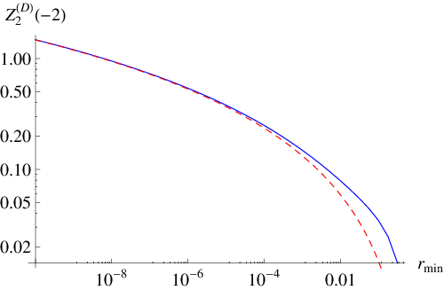
\displaystyle Z_{2}^{(D)}(-2)

\displaystyle\approx

\displaystyle\frac{\log^{2}(r_{min})}{360}-\frac{\zeta(3)}{8\log(r_{min})}-\frac{\pi^{4}}{360\log^{2}(r_{min})}+\dots

(124)

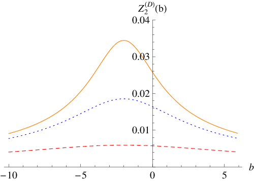
In Fig.3 we plot the sum rule $Z_{2}^{(D)}(b)$ at three different values of $r_{min}$ as a functions of $b$ . The curve is symmetric with respect to the axis $b=-2$ , as a result of the isospectrality discussed earlier.

In Fig.4 we plot the sum rule $Z_{2}^{(D)}(-2)$ as a function of $r_{min}$ (solid line); the dashed line is the asymptotic behavior of eq.(124).

6 Conclusions

We have extended the results of Ref. [15] to two dimensional domains of arbitrary shape and density; we have derived a general expression for the sum rule of integer order $n$ in terms of the Green’s functions of the homogeneous problem and we have proved that the sum rule of any integer order can be expressed in terms of a single series for the case in which the inhomogeneity is only along a direction. We have also discussed the generalization of these results to higher dimensions.

As an application of the formulas that we have derived, we have calculated the sum rules for an homogeneous circular annulus, for a homogeneous circular sector and for a circular annulus with a radially varying density. We have found explicit expressions for the sum rules of a circular annulus subject to different boundary conditions and with an infinitesimal internal hole: in the case of Dirichlet boundary conditions on the external border we have proved that the sum rules tend to the corresponding sum rules for the unit circle.

The possibility of obtaining exact expressions for the sum rules of the eigenvalues of the negative laplacian on arbitrary domains may be exploited to estimate the higher order coefficients in Weyl’s asymptotic law. This aspect would provide a natural extension of the present work and we plan to consider it in the future. As we have discussed in [15], following [5], the sum rules may be used to provide rigorous upper and lower bounds to the lowest eigenvalue.

Acknowledgements

This research was supported by the Sistema Nacional de Investigadores (México).

References

[1] P. Amore, J. Math. Phys. 53, 123519 (2012)
[2] A. Voros, Nucl. Phys.B 165, 209 (1980)
[3] A. Voros, J.Phys.A 32, 1301-1311 (1999)
[4] F. Steiner, Phys.Lett.B 159, 397-402 (1985)
[5] M.V.Berry, J.Phys.A 19, 2281-2296 (1986)
[6] F. Steiner, Fortschr. Phys.35, 87-114 (1987)
[7] E.Elizalde, S.Leseduarte and A.Romeo, J.Phys.A 26, 2409-2419 (1993)
[8] F. Steiner, Phys.Lett.B 188, 447-454 (1987)
[9] W. Arendt, R. Nittka, W. Peter and F.Steiner, "Weyl’s law: spectral properties of the Laplacian in Mathematics and Physics", in "Mathematical Analysis of Evolution, Information and Complexity", edited by W. Arendt et al., Wiley-VCH (2009), 1-71
[10] R.E. Crandall, J.Phys.A 29, 6795-6816 (1996)
[11] A.A. Kvitsinsky, J.Phys.A 29, 6379-6393 (1996)
[12] B. Dittmar and M. Hantke, Annales UMCS, Mathematica, 65(2), 29-44 (2011)
[13] G.A. Mezincescu, J.Phys.A 33, 4911 (2000)
[14] C.M.Bender and Q.Wang, J.Phys.A 34, 3325 (2001)
[15] P. Amore, "Exact sum rules for inhomogeneous strings" (2013)
[16] C. Itzykson, P. Moussa and J.M.Luck, J.Phys.A 19, L111-L115 (1986)
[17] B. Dittmar, Math. Nachr. 237, 45 – 61 (2002)
[18] Jackson, John David. Classical electrodynamics, Third edition, New York: Wiley, 1998.
[19] C. Alvarado and P. Amore, J. Math. Phys. 52, 063516 (2011)
[20] H.P.W. Gottlieb, ANZIAM Journal 47, C152-C167 (2006)
[21] H.P.W. Gottlieb, IMA Journal of Applied Mathematics 71, 583-589 (2006)
[22] P. Amore, J. Math. Phys. 51, 052105 (2010)