跳到论文正文
W Papers独立论文阅读器 arXiv:1302.4339 论文正文 计算阅读时间 · 0%
引用这篇论文根据当前论文元数据生成,正式投稿前建议核对。


License: arXiv.org perpetual non-exclusive license
arXiv:1302.4339v1 [math.PR] 18 Feb 2013


Diffusivity in multiple scattering systems

Timothy Chumley  Note: Washington University, Department of Mathematics, Campus Box 1146, St. Louis, MO 63130    Renato Feres11footnotemark: 1    Hong-Kun Zhang Note: Department of Mathematics and Statistics, University of Massachusetts, Amherst, MA 01003, USA
August 24, 2026
Abstract

Abstract

We consider random flights of point particles inside nn-dimensional channels of the form ℝk×𝔹n−k\mathbb{R}^{k}\times\mathbb{B}^{n-k}, where 𝔹n−k\mathbb{B}^{n-k} is a ball of radius rr in dimension n−kn-k. The particle velocities immediately after each collision with the boundary of the channel comprise a Markov chain with a transition probabilities operator PP that is determined by a choice of (billiard-like) random mechanical model of the particle-surface interaction at the “microscopic” scale. Our central concern is the relationship between the scattering properties encoded in PP and the constant of diffusivity of a Brownian motion obtained by an appropriate limit of the random flight in the channel. Markov operators obtained in this way are natural (definition below), which means, in particular, that (1) the (at the surface) Maxwell-Boltzmann velocity distribution with a given surface temperature, when the surface model contains moving parts, or (2) the so-called Knudsen cosine law, when this model is purely geometric, is the stationary distribution of PP. We show by a suitable generalization of a central limit theorem of Kipnis and Varadhan how the diffusivity is expressed in terms of the spectrum of PP and compute, in the case of 22-dimensional channels, the exact values of the diffusivity for a class of parametric microscopic surface models of the above geometric type (2).

1 Introduction and general definitions

We consider mathematical models of particle-surface systems involving multiple, or iterated, (classical) scattering. The purpose of this section is to motivate the main question regarding these systems and to introduce a few definitions needed to informally explain our results. More detailed statements will be given in the course of the paper.

1.1 An idealized experiment and the main question

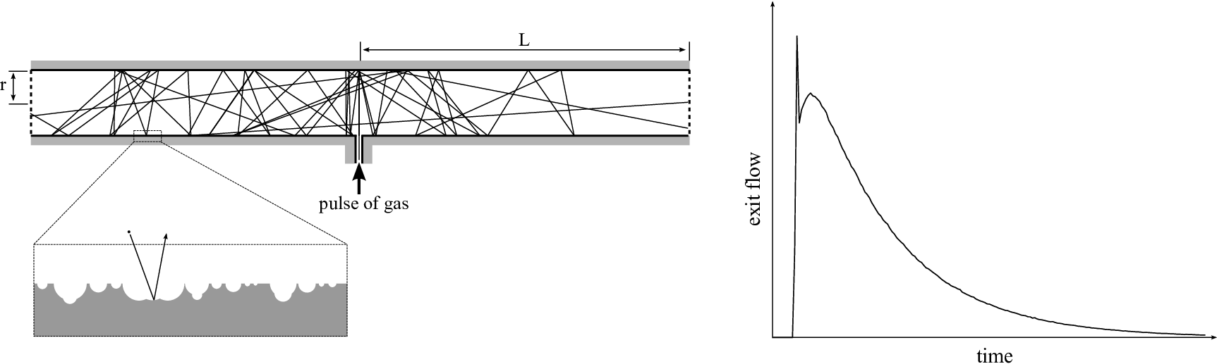
Figure 1.1 depicts an ideal experiment in which a small amount of gas composed of point-like, non-interacting masses is injected into a (for simplicity of exposition 22-dimensional) channel and the amount of outflowing gas per unit time is recorded. The graph on the right-hand side shows a typical exit flow curve. Possible gas transport characteristics that can be obtained from such an experiment are the mean value and higher moments of the molecular time of escape.

The central question then is: what can these time characteristics of the gas outflow tell us about the microscopic interaction (i.e., scattering properties) between gas molecules and the surface of the plates?

For a more precise formulation of this question, we begin by describing the classical surface scattering operators that model the microscopic collisions of the point mass. We refer to the boundary of the channel region as the (wall) surface, irrespective of its actual dimension.

Let ℍ\mathbb{H} denote the upper-half plane, consisting of vectors (v1,v2)(v_{1},v_{2}) with positive second component. Elements of ℍ\mathbb{H} represent velocities of a point mass immediately after a collision with the surface. By identifying (v1,−v2)(v_{1},-v_{2}) and (v1,v2)(v_{1},v_{2}), we may regard pre-collision velocities as also being in ℍ\mathbb{H}. A collision event is then specified by a measurable map v∈ℍ↦ηv∈𝒫⁡(ℍ),v\in\mathbb{H}\mapsto\eta_{v}\in\mathcal{P}(\mathbb{H}), where 𝒫⁡(ℍ)\mathcal{P}(\mathbb{H}) indicates the space of probability measures on the upper-half plane. The measurability condition is understood as follows: For every essentially bounded Borel measurable function ϕ\phi on ℍ\mathbb{H}, the function

v↦(P​ϕ)​(v):=∫ℍϕ⁡(u)​d​ηv​(u)v\mapsto(P\phi)(v):=\int_{\mathbb{H}}\phi(u)\,d\eta_{v}(u)

is also measurable. We refer to PP as the collision operator. This operator specifies the transition probabilities of Markov chains with state space ℍ\mathbb{H} giving the sequence of post-collision velocities from which the molecular random flight inside the channel can be obtained.
Refer to caption

Figure 1.1: Idealized experiment in which a small pulse of gas is injected into a 22-dimensional channel and the gas outflow is recorded. The graph on the right represents the rate at which gas escapes. From this function it is possible to derive mean exit time of escape τ\tau. The main problem is to relate easily measured properties of the gas outflow, such as τ\tau, to the microscopic scattering characteristics of the channel surface.

If now τ=τ⁡(L,r,s)\tau=\tau(L,r,s) denotes the expected exit time of the random flight, where ss is the molecular root-mean square velocity, then a more restricted form of the general question is to understand how τ\tau depends on PP. (This expected exit time is easily measured in actual experiments involving gas diffusion using the rate of gas outflow as represented on the right hand side of Figure 1.1; see, for example, [22] for so-called TAP-experiments in chemical kinetics.)

Although the analysis of PP is generally simpler in dimension 22, an interesting complication arises here that is not present in the case of a 33-dimensional cylinder; namely, with respect to the stationary distribution of velocities for natural collision operators (see the next subsection), molecular displacement between collisions has infinite variance and standard central limit theorems for Markov chains do not apply. The same is true for the random flight in the region ℝ2×[−r,r]\mathbb{R}^{2}\times[-r,r] between two parallel plates. In this regard, the random flight in a 33-dimensional cylindrical channel is simpler. (For an early study of two parallel plates case, see in [6].) Infinite variance of the in-between collisions displacements requires a generalization of the central limit theorem of Kipnis and Varadhan in [20] that is proved in this paper.

Now, from an appropriate central limit theorem we obtain for τ\tau the asymptotic expression

(1.1) τ⁡(L,r,s)∼L2𝒟​ln⁡(Lr)\tau(L,r,s)\sim\frac{L^{2}}{\mathcal{D}\ln\left(\frac{L}{r}\right)}

for long channels in dimension 22, i.e., for large values of L/rL/r, where 𝒟=𝒟⁡(r,s)\mathcal{D}=\mathcal{D}(r,s) is the diffusivity of a limit Brownian motion. Therefore, a more specific formulation of the problem is to understand how properties of the collision operator are reflected on 𝒟\mathcal{D}. A simple dimensional argument given in Subsection 2.2 shows that

𝒟⁡(r,s)=4​r​sπ​η,\mathcal{D}(r,s)=\frac{4rs}{\pi}\eta,

where η\eta only depends on the scattering characteristics at the microscopic scale determined by PP. The choice of constants will become clear shortly.

The typical, but not the only type of operator we consider here is defined by a choice of microscopic contour of the channel wall surface, as suggested by Figure 1.1. The main problem then amounts to finding the functional dependence of η\eta on geometric parameters of the surface microstructure. These parameters are scale invariant and are typically length ratios and angles. The presence of the logarithmic term in τ\tau is related to some surprising properties of 𝒟\mathcal{D}, as will be noted below, and for this reason we give somewhat greater prominence to the two-dimensional set-up in this paper.

1.2 Natural collision operators and microstructures

Let d​V​(v)dV(v) denote the standard volume element on nn-dimensional half-space ℍ:=ℍn\mathbb{H}:=\mathbb{H}^{n} and define the probability measure

d​μβ​(v)=2​π​(β​M2​π)n+12​⟨v,en⟩​exp⁡(−β​M2​|v|2)​d​V​(v).d\mu_{\beta}(v)=2\pi\left(\frac{\beta M}{2\pi}\right)^{\frac{n+1}{2}}\langle v,e_{n}\rangle\exp\left(-\frac{\beta M}{2}|v|^{2}\right)\,dV(v).

on ℍ\mathbb{H}. We refer to μβ\mu_{\beta} as the surface Maxwellian, or surface Maxwell-Boltzmann distribution, with parameter β\beta and particle mass MM. Here, ⟨v,en⟩\langle v,e_{n}\rangle denotes the standard inner product (dot product) of v∈ℍnv\in\mathbb{H}^{n} and the unit normal vector, ene_{n}, to the boundary surface at the origin. We often denote this normal vector by n=enn=e_{n}. It will be clear in context whether nn refers to dimension or to this normal vector.

In physics textbooks, β=1/κ​T\beta=1/\kappa T, where TT is absolute temperature and κ\kappa is the Boltzmann constant. A simple integral evaluation shows that the mean squared post-collision speed with respect to μβ\mu_{\beta} is

sm​s2:=∫ℍn|v|2​d​μβ​(v)=n+1β​M.s_{ms}^{2}:=\int_{\mathbb{H}^{n}}|v|^{2}\,d\mu_{\beta}(v)=\frac{n+1}{\beta M}.

Another distribution of collision velocities that arises naturally is concentrated on an hemisphere S+​(s):={v∈ℍ:|v|=s}S^{+}(s):=\{v\in\mathbb{H}:|v|=s\}; it is defined by

d​μ​(v)=Γ⁡(n+12)sn​πn−12​⟨v,n⟩​d​Vsph​(v)d\mu(v)=\frac{\Gamma\left(\frac{n+1}{2}\right)}{s^{n}\pi^{\frac{n-1}{2}}}\langle v,n\rangle\,dV_{\text{\tiny sph}}(v)

where d​Vsph​(v)dV_{\text{\tiny sph}}(v) is the volume element on the hemisphere of radius ss induced from the ambient Euclidean space. In dimension 22, d​μ​(v)=12​s2​⟨v,n⟩​d​S​(v),d\mu(v)=\frac{1}{2s^{2}}{\langle v,n\rangle}\,dS(v), where d​SdS indicates arclength element on S+​(s)S^{+}(s). Equivalently, d​μ​(θ)=12​cos⁡θ​d​θ,d\mu(\theta)=\frac{1}{2}\cos\theta d\theta, where θ\theta is the angle between vv and the normal vector nn.

Definition 1 (Natural collision operators).

The collision operator PP will be called natural if one of the following holds: (a) μβ\mu_{\beta} is the unique stationary distribution for PP, for some β\beta; (b) the process defined by PP does not change the particle speed and μ\mu is a stationary probability measure for PP for all ss. If case (a) holds we say that the surface with associated operator PP has temperature T=1/κ​βT=1/\kappa\beta; in case (b) we say that PP represents a random reflection. In addition, we demand in both cases that PP and its stationary probability satisfy the detailed balance condition (see equation (20.5) of [23]). We use ν\nu throughout the paper to indicate either μβ\mu_{\beta} or μ\mu.

Refer to caption

Figure 1.2: A periodic microstructure without moving parts. The cube containing a period of the microstructure defines a cell; the point in a kk-dimensional torus 𝕋k\mathbb{T}^{k} at which the particle enters a typical cell is assumed to be a uniform random variable. The particle enters with pre-collision velocity vv and exits with post-collision velocity VV. The corresponding PP describes a random reflection, as defined in the text.

The natural operators of particular interest to us are those defined by a choice of surface microscopic structure. We briefly described them here. (See [14], [15], [16], and [17] for more details.) By surface (micro-)structure we mean that the channel wall’s surface has a periodic relief composed of cells, each consisting of a mechanical system of moving masses or more simply a fixed geometric shape with no moving parts. (Natural collision operators specified by the former correspond to part (a) of the definition, while the latter correspond to part (b).) Moreover, the wall system, mechanical or purely geometric, is assumed to be at a “microscopic” length scale that, by definition, is incommensurate with that of the channel defined, say, by the radius of the ball factor 𝔹n−k\mathbb{B}^{n-k}. At a collision event, the point particle enters a cell of the wall system, undergoes one or more deterministic collisions with it, transferring energy between wall and particle in case (a), and leaves with a seemingly—from the perspective of the channel length scale—random velocity VV. (See Figure 1.2.) Because of this assumption of incommensurability between the micro and macro scales, the relevant scattering properties specifying PP are invariant under homotheties. Thus in dimension 22 we may, when convenient, assume that the width of each cell is 1.

This incommensurability also dictates our assumption that the particle position on the entrance of a cell at the beginning of a collision event is a uniformly distributed random variable. When the wall system has moving parts, the kinetic state of the cell at the moment the particle enters a cell is also drawn from a fixed probability distribution (a canonical Gibbs state at temperature TT). Under these assumptions, VV is an actual random variable and it can be shown (see [14]) that the associated collision operator PP is natural according to Definition 1. The periodicity condition is not essential—all the basic facts discussed here hold, for example, for random structures, defined as probabilistic mixtures of periodic micro-structures.

The operator PP can be expressed as follows. Let ff be, say, a continuous bounded function on ℍ\mathbb{H}, and let V+V_{+} be the random velocity immediately after the collision of a particle with incoming velocity V−=vV_{-}=v. Then

(P​f)​(v)=𝔼⁡[f⁡(V+)|V−=v].(Pf)(v)=\mathbb{E}[f(V_{+})|V_{-}=v].

For example, in the purely geometric case of random reflections in dimension 22, PP is given by

(P​f)​(θ)=∫01f⁡(Ψθ​(r))​𝑑r(Pf)(\theta)=\int_{0}^{1}f\left(\Psi_{\theta}(r)\right)dr

where Ψθ​(r)\Psi_{\theta}(r) is the angle VV makes with the normal vector nn and r∈[0,1]r\in[0,1] is the position at which the particle enters a cell before collision. A similar integral over 𝕋k\mathbb{T}^{k} defines PP in general dimension.

Refer to caption

Figure 1.3: An example of a wall system with moving parts. Mass m0m_{0} can move freely up and down, bouncing off elastically against the fixed floor and an upper limit that is permeable to m1m_{1}.

Figure 1.3 illustrates a wall system with micro-structure having moving parts. The periodic relief is assigned a mass m0m_{0} and can move vertically and freely over a short range of distances [0,a][0,a] from the fixed base, bouncing off elastically at the lower and upper limits. The point particle of mass m1m_{1} enters the wall system with velocity vv at a uniformly random location along [0,1][0,1]. Upon entrance, the velocity of the wall is assumed to be normally distributed with mean 00 and a given variance σ2\sigma^{2}, where m0​σ2m_{0}\sigma^{2} is proportional to the wall temperature; the particle then goes on to interact deterministically with the wall, leaving with random velocity VV. This is a very special example of wall system for which PP is natural. For other examples and details about random billiards with microstructures omitted here see [14]. See also [18] for a detailed analysis of this and other examples in the context of stochastic processes in velocity space ℍ\mathbb{H} having stationary measure μβ\mu_{\beta} or μ\mu.

If we assume that the wall is static and has infinite mass, the system of the figure becomes purely geometric and the particle mass plays no role. In this case the operator PP describes a random reflection. We refer to the subclass of natural operators derived from microscopic structures (either static or having moving parts, with arbitrary surface contours) as operators associated to surface microstructures. An interesting question suggested by [1] is whether general natural operators are limits of operators associated to surface microstructures.

Proposition 1.

The operators for the classes of examples of Figures 1.2 and 1.3 are natural.

Proof.

See [14, 18] for proofs of these basic issues related to stationary measures and more examples. ∎

Occasionally, ν\nu will stand for either of the two measures μβ\mu_{\beta} or μ\mu of Definition 1. Because PP and ν\nu are assumed to satisfy the detailed balance condition, PP is a self-adjoint operator of norm 11 on L2​(ℍ,ν)L^{2}(\mathbb{H},\nu). A further assumption for the main results below is that PP be quasi-compact; that is, the spectral radius of PP restricted to the orthogonal complement of the constant function in L2​(ℍ,ν)L^{2}(\mathbb{H},\nu) is strictly less than 11. Quasi-compactness for natural collision operators for the types of systems illustrated in Figure 1.2 is known to hold in a number of cases. The static version of the system of Figure 1.2 (for the specific shape shown in the figure) has this property (see [16], [17]), and the operator for the one-dimensional version of the moving wall is known to be compact (see [14]); the case of the two-dimensional moving wall is still open. Further examples of shapes of systems of the static type having quasi-compact PP will be provided later in this paper.

Noting the two roles of PP, as a self-adjoint operator on L2​(ℍ,ν)L^{2}(\mathbb{H},\nu) and as a Markov transition probabilities operator, a useful characterization of powers of PP is as follows. Let V0,V1,…V_{0},V_{1},\dots be a stationary Markov chain with transitions PP and initial distribution ν\nu and let Ψ,Φ∈L2​(ℍ,ν)\Psi,\Phi\in L^{2}(\mathbb{H},\nu). Then it is not difficult to show that

⟨Ψ,Pk​Φ⟩=𝔼ν​[Ψ⁡(Vi)​Φ​(Vi+k)]\left\langle\Psi,P^{k}\Phi\right\rangle=\mathbb{E}_{\nu}[\Psi(V_{i})\Phi(V_{i+k})]

for any i≥0i\geq 0, where 𝔼ν\mathbb{E}_{\nu} indicates expectation given that V0V_{0} is distributed according to ν\nu.

2 Random flight and diffusivity

2.1 Between-collisions displacements and times

The logarithmic term in Equation 1.1 is a special feature of the random billiard process in regions bounded by parallel plates in arbitrary dimensions (in particular 22-dimensional channels bounded by a pair of parallel lines), and it is not present in the more typical cylindrical channel region ℝk×𝔹n−k\mathbb{R}^{k}\times\mathbb{B}^{n-k} for k=1,…,n−2k=1,\dots,n-2. Ultimately, this is due to the mean square displacements being infinite in the two-plates case and finite in the other cases, as will be seen later. This elementary but key observation is highlighted in the next proposition.

Let 𝒞:=𝒞n:=ℝk×𝔹n−k\mathcal{C}:=\mathcal{C}^{n}:=\mathbb{R}^{k}\times\mathbb{B}^{n-k} denote the channel region. Of special interest are the low dimensional cases: n−k=1n-k=1, for n=2,3n=2,3 (two-dimensional channels and slabs in dimension 33) and k=1k=1, n=3n=3 (cylindrical channels in dimension 33). Let ℍq\mathbb{H}_{q} represent the upper-half space consisting of vectors v∈Tq​𝒞v\in T_{q}\mathcal{C}, q∈∂𝒞q\in\partial\mathcal{C}, such that ⟨n,v⟩>0\langle n,v\rangle>0, where nn is the unit vector in ℍq\mathbb{H}_{q} perpendicular to ∂𝒞\partial\mathcal{C} and ⟨⋅,⋅⟩\langle\cdot,\cdot\rangle is the inner product given by restriction of the standard dot product in ℝn\mathbb{R}^{n}. If q′q^{\prime} is the next collision point of the trajectory t↦q+t​vt\mapsto q+tv, let Z⁡(v)Z(v) denote the natural projection to the “horizontal” factor ℝk\mathbb{R}^{k} of the vector q′−q∈ℝnq^{\prime}-q\in\mathbb{R}^{n}. We refer to Z⁡(v)Z(v) as the (horizontal) displacement vector for the given vv. See Figure 2.1. The time of free flight between the collisions at qq and q′q^{\prime} will be indicated by τb​(v)\tau_{b}(v).

Refer to caption

Figure 2.1: The between-collisions displacement vector Z⁡(v)Z(v), where vv is the post-collision velocity at a boundary point of the channel region. The time between two consecutive collisions is denoted in this section τb​(v)\tau_{b}(v).
Proposition 2.

Let ν\nu be either of the two probability measures of Definition 1 (denoted there μβ\mu_{\beta} and μ\mu). This is a probability measure on ℍ≅Tq​𝒞\mathbb{H}\cong T_{q}\mathcal{C} (concentrated on a hemisphere in the case of μ\mu), for a given collision point q∈∂𝒞q\in\partial\mathcal{C}. Let ZaZ_{a} denote the product of ZZ and the indicator function of the cone ℍ⁡(a):={v∈ℍ:|Z⁡(v)|≤a​r}\mathbb{H}(a):=\{v\in\mathbb{H}:|Z(v)|\leq ar\} for a>0a>0. Also define for any unit vector u∈ℝku\in\mathbb{R}^{k} the orthogonal projection Zau:=⟨u,Za⟩Z_{a}^{u}:=\langle u,Z_{a}\rangle. Then, if n−k≥2n-k\geq 2,

𝔼ν​[(Zu)2]=lima→∞𝔼ν​[(Zau)2]=4​r2(n−k)2−1.\mathbb{E}_{\nu}\left[\left(Z^{u}\right)^{2}\right]=\lim_{a\rightarrow\infty}\mathbb{E}_{\nu}\left[\left(Z^{u}_{a}\right)^{2}\right]=\frac{4r^{2}}{(n-k)^{2}-1}.

If n−k=1n-k=1, then the asymptotic expression

𝔼ν​[(Zau)2]∼4​r2​ln⁡a\mathbb{E}_{\nu}\left[\left(Z_{a}^{u}\right)^{2}\right]\sim{4r^{2}}\ln a

holds. The expected time of free flight τb\tau_{b} (here ‘b’ is for ‘between collisions’) is finite for both types of measures and n−k≥1n-k\geq 1. For the stationary measure μ\mu supported on the hemisphere of speed ss,

𝔼μ​[τb]=2​r​πs⁡(n−k)​Γ⁡(n+12)Γ⁡(n2).\mathbb{E}_{\mu}\left[\tau_{b}\right]=\frac{2r\sqrt{\pi}}{s(n-k)}\frac{\Gamma\left(\frac{n+1}{2}\right)}{\Gamma\left(\frac{n}{2}\right)}.

For μβ\mu_{\beta}, the corresponding expression is

𝔼μβ​[τb]=rn−k​2​π​β​M\mathbb{E}_{\mu_{\beta}}\left[\tau_{b}\right]=\frac{r}{n-k}\sqrt{2\pi\beta M}

where MM is particle mass.

For a sketch of the proof, see Section 5.1.

Before considering random flights in 𝒞\mathcal{C}, we need to mention a technical point of geometric interest that only arises in dimensions n>3n>3, having to do with whether the operator PP actually gives rise to a well-defined process in 𝒞\mathcal{C}. The issue is that in order for a fixed PP to induce a scattering operator at each Tq​𝒞T_{q}\mathcal{C}, q∈∂𝒞q\in\partial\mathcal{C}, we need to be able to identify the positive part (say, inward pointing) of this tangent space with the half-space ℍ={v∈ℝn:⟨v,en⟩>0}\mathbb{H}=\{v\in\mathbb{R}^{n}:\langle v,e_{n}\rangle>0\}. Such identification amounts to specifying an orthonormal frame on the tangent space at each boundary point, which provides the information of how the model microstructure is “aligned” with the channel wall. Introducing a frame field on ∂𝒞\partial\mathcal{C} has, however, the effect that the scattering operator PqP_{q} at each boundary point qq becomes a conjugate of PP under an orthogonal transformation, rather than PP itself. For all the cases in dimensions 22 and 33, namely (n=2,k=1),(n=3,k=1),(n=3,k=2)(n=2,k=1),(n=3,k=1),(n=3,k=2), there is a natural frame (the parallel transported frame over the boundary of the channel) with respect to which Pq=PP_{q}=P for all qq. In the general case, Tq​𝒞T_{q}\mathcal{C} has a canonical orthogonal decomposition into a “horizontal” part, naturally identified with ℝk\mathbb{R}^{k}, and a vertical part that splits orthogonally into the normal direction ℝ​nq\mathbb{R}n_{q} and the complement 𝕍q\mathbb{V}_{q} of dimension n−k−1n-k-1. We can now understand the issue as follows: Let vv be a velocity vector of a particle that emerges from a collision at q∈∂𝒞q\in\partial\mathcal{C} and will collide again next at q′q^{\prime}. In order that the Markov chain in velocity space be given by iterates of the same operator PP, we need a field of orthonormal frames with respect to which vv, at qq, and its mirror reflection at q′q^{\prime} have the same representation as vectors in ℝn\mathbb{R}^{n}. The components of these two vectors in 𝕍q⟂\mathbb{V}^{\perp}_{q} and 𝕍q′⟂\mathbb{V}^{\perp}_{q^{\prime}}, respectively, agree if we choose the canonical (parallel) frame, but on the subspaces 𝕍q\mathbb{V}_{q} themselves no such frame exists in general. With this in mind, and to avoid complicating the picture by introducing such frame fields as additional structure, we simply assume without further mention that PP is 𝕍\mathbb{V}-isotropic, that is, it is invariant under conjugation by orthogonal linear maps that restrict to the identity on ℝk⊕ℝ​en\mathbb{R}^{k}\oplus\mathbb{R}e_{n}. Notice that this assumption is vacuous in dimensions 22 and 33.

2.2 Diffusivity, spectrum and mean exit time

Let X¯t\overline{X}_{t}, t≥0t\geq 0, be a piecewise linear path in the channel region 𝒞\mathcal{C} describing a random flight governed by a natural collision operator PP. Recall that PP is a self-adjoint operator on L2​(ℍ,ν)L^{2}(\mathbb{H},\nu). We assume throughout that PP is quasi-compact. (This is one of the conditions needed for Theorem 2, below.)

We wish to consider a diffusion process in ℝk\mathbb{R}^{k} obtained by an appropriate scaling limit of the projection of X¯t\overline{X}_{t} to the ℝk\mathbb{R}^{k} factor of 𝒞\mathcal{C}. Let this projection be denoted XtX_{t}, and assume X0=0X_{0}=0. The sequence of post-collision velocities of X¯t\overline{X}_{t} is a stationary Markov chain V0,V1,…V_{0},V_{1},\dots, with initial distribution ν\nu. The displacement vectors, previously defined, are random variables Z0,Z1,…Z_{0},Z_{1},\dots. Thus XtX_{t}, at collision times, are sums of the ZiZ_{i}. The aa-scaled random flight is defined as follows. Let h⁡(a)h(a), a>0a>0, be

h⁡(a)={a for ​n−k≥2a/log⁡a for ​n−k=1.h(a)=\begin{cases}a&\text{ for }n-k\geq 2\\ a/\log a&\text{ for }n-k=1.\end{cases}

Define the scaled channel system with scale parameter a>0a>0 to be the channel system with radius r/ar/a and root-mean-square velocity h⁡(a)​sm​sh(a)s_{ms}. (If ν=μ\nu=\mu, sm​ss_{ms} is the constant speed throughout the process and if ν=μβ\nu=\mu_{\beta}, sm​s2=(n+1)/β​Ms^{2}_{ms}=(n+1)/\beta M.) The random flight paths and their projection are defined as the paths for the aa-system. We denote them by X¯a,t\overline{X}_{a,t} and Xa,tX_{a,t}, respectively. The aa-scaled free displacement with post-collision velocity vector vv is a−1​Z​(v)a^{-1}Z(v), and the displacements associated to the VjV_{j} are a−1​Zja^{-1}Z_{j}. For any τ>0\tau>0, over a time interval [0,τ][0,\tau], the number of collisions of X¯t\overline{X}_{t} with ∂𝒞\partial\mathcal{C} will written NτN_{\tau}. For the aa-scaled system this number is Na,τ:=Na​h​(a)​τN_{a,\tau}:=N_{ah(a)\tau}. For the cases in which n−k=1n-k=1, when 𝔼ν​[|Z|2]\mathbb{E}_{\nu}\left[|Z|^{2}\right] is infinite, it will be necessary to also consider the aa-truncation ZaZ_{a} of ZZ introduced above in Proposition 2. The aa-scaled aa-truncation of ZZ and ZjZ_{j} will be written a−1​Zaa^{-1}Z_{a} and a−1​Za,ja^{-1}Z_{a,j}. Finally, we will like to follow the projected random flight along an axis set by a unit vector u∈ℝku\in\mathbb{R}^{k}. Thus we define ZuZ^{u}, XtuX^{u}_{t}, ZauZ_{a}^{u}, etc., to be the orthogonal projections of ZZ, XtX_{t}, ZaZ_{a}, etc., on ℝ​u\mathbb{R}u.

Theorem 1 below gives conditions under which Xa,tX_{a,t} converges to Brownian motion for large aa. In this subsection, we wish to focus on the variance (or diffusivity) of the limit Brownian motion, and provide an interpretation of this constant in a way that does not make use of the physically somewhat artificial scaling just introduced. The precise conditions for the diffusion limit to exist when ZZ has infinite variance relative to ν\nu (i.e., for n−k=1n-k=1) are not yet fully clear; for Theorem 1 we make the following additional assumption that will be verified in the examples discussed later.

Assumption 1.

Define for γ>1\gamma>1 the set ℍγ​(a):={v∈ℍ:|Zu​(v)|≤a​r/logγ⁡a}\mathbb{H}^{\gamma}(a):=\{v\in\mathbb{H}:|Z^{u}(v)|\leq ar/\log^{\gamma}a\} and let Za,γ,juZ^{u}_{a,\gamma,j} be the product of ZjuZ^{u}_{j} by the indicator function of  ℍγ​(a)\mathbb{H}^{\gamma}(a). Then, for any t>0t>0,

lima→∞𝔼ν​[(1a​∑j=0Na,tZa,γ,ju)2]\lim_{a\rightarrow\infty}\mathbb{E}_{\nu}\left[\left(\frac{1}{a}\sum_{j=0}^{N_{a,t}}Z^{u}_{a,\gamma,j}\right)^{2}\right]

exists for all unit vectors u∈ℝku\in\mathbb{R}^{k}.

This assumption, which will only be needed when n−k=1n-k=1, will be explained later in the context of Theorems 2 and 3. It is not needed for n−k≥2n-k\geq 2, when ZZ has finite variance and Theorem 1 is for the most part a consequence of well known limit theorems, in particular the central limit theorem for reversible Markov chains as formulated by Kipnis and Varadhan in [20].

Theorem 1 (Diffusion limit).

Let PP be quasi-compact and, if n−k=1n-k=1, suppose that Assumption 1 holds. Then the aa-scaled projected random path Xa,tuX^{u}_{a,t}, for a unit vector u∈ℝku\in\mathbb{R}^{k}, converges weakly as a→∞a\rightarrow\infty to a Brownian motion in ℝ​u\mathbb{R}u with diffusion constant 𝒟u\mathcal{D}^{u} further specified below. In particular, Xa,tuX^{u}_{a,t} converges in distribution for each t>0t>0 to a normal random variable in ℝ​u\mathbb{R}u with mean 00 and variance t​𝒟ut\mathcal{D}^{u}. The following statements concerning 𝒟u\mathcal{D}^{u} also hold:

  1. 1.

    For the purpose of having a baseline value for 𝒟u\mathcal{D}^{u}, suppose that PP maps probability measures to ν\nu. In other words, let the velocity process on ℍ\mathbb{H} be i.i.d. with probability measure ν\nu. Let n−k≥2n-k\geq 2. Then, denoting the constant 𝒟0u\mathcal{D}_{0}^{u} in this special case,

    𝒟0u=42​π​(n+1)​n−k(n−k)2−1​r​sm​s\mathcal{D}_{0}^{u}=\frac{4}{\sqrt{2\pi(n+1)}}\frac{n-k}{(n-k)^{2}-1}rs_{ms}

    when ν=μβ\nu=\mu_{\beta} and

    𝒟0u=2π​Γ⁡(n2)Γ⁡(n+12)​n−k(n−k)2−1​r​s\mathcal{D}^{u}_{0}=\frac{2}{\sqrt{\pi}}\frac{\Gamma\left(\frac{n}{2}\right)}{\Gamma\left(\frac{n+1}{2}\right)}\frac{n-k}{(n-k)^{2}-1}rs

    when ν=μ\nu=\mu. Recall that sm​ss_{ms} is the root-mean-square velocity for μβ\mu_{\beta}, and that μ\mu is concentrated on the hemisphere of radius ss in ℍ\mathbb{H}. Being independent of uu, we denote these values by 𝒟0\mathcal{D}_{0}.

  2. 2.

    For n−k=1n-k=1, the baseline diffusivities are

    𝒟0=42​π​(n+1)​r​sm​s\mathcal{D}_{0}=\frac{4}{\sqrt{2\pi(n+1)}}rs_{ms}

    when ν=μβ\nu=\mu_{\beta} and

    𝒟0=2π​Γ⁡(n2)Γ⁡(n+12)​r​s\mathcal{D}_{0}=\frac{2}{\sqrt{\pi}}\frac{\Gamma\left(\frac{n}{2}\right)}{\Gamma\left(\frac{n+1}{2}\right)}rs

    when ν=μ\nu=\mu, supported on the hemisphere of radius ss.

  3. 3.

    The diffusion constant for a general PP can now be written as 𝒟u=η⁡(u)​𝒟0\mathcal{D}^{u}=\eta(u)\mathcal{D}_{0}, where η⁡(u)\eta(u) has the following expression in terms of the spectrum of PP. First consider the case n−k≥2n-k\geq 2 and define a probability measure on the spectrum by

    Πu​(d​λ):=‖Zu‖−2​⟨Zu,Π⁡(d​λ)​Zu⟩,\Pi^{u}(d\lambda):=\|Z^{u}\|^{-2}\left\langle Z^{u},\Pi(d\lambda)Z^{u}\right\rangle,

    where Π\Pi is projection-valued spectral measure associated to PP and the inner product and norm are those of L2​(ℍ,ν)L^{2}(\mathbb{H},\nu). Then

    (2.1) η⁡(u)=∫−111+λ1−λ​Πu​(𝑑λ).\eta(u)=\int_{-1}^{1}\frac{1+\lambda}{1-\lambda}\,\Pi^{u}(d\lambda).

    Notice that η⁡(u)\eta(u) is quadratic in uu. Now suppose n−k=1n-k=1 and define for each aa the probability measure

    Πau​(d​λ):=‖Zau‖−2​⟨Zau,Π⁡(d​λ)​Zau⟩\Pi^{u}_{a}(d\lambda):=\|Z^{u}_{a}\|^{-2}\left\langle Z^{u}_{a},\Pi(d\lambda)Z^{u}_{a}\right\rangle

    on the spectrum and the function ηa​(u)=∫−111+λ1−λ​Πau​(𝑑λ)\eta_{a}(u)=\int_{-1}^{1}\frac{1+\lambda}{1-\lambda}\Pi_{a}^{u}(d\lambda). Then the limit lima→∞ηa​(u)\lim_{a\rightarrow\infty}\eta_{a}(u) exists and defines a quadratic function η⁡(u)\eta(u) of uu.

Proof.

The limit theorems in probability theory we require are standard in the case n−k≥2n-k\geq 2 and will be proved later for n−k=1n-k=1 in Theorems 2 and 3. Here we only indicate how 𝒟0\mathcal{D}_{0} and the expression for η⁡(u)\eta(u) in terms of the spectrum of PP are obtained.

Recall that Na,t=Na​h​(a)​tN_{a,t}=N_{ah(a)t} is the number of collisions of the aa-scaled random flight with the boundary of the (aa-scaled) channel region during time interval [0,t][0,t]. Let τj\tau_{j} denote the time duration of the step with (non-scaled) displacement ZjZ_{j}. Then, as

(τ0+⋯+τNT−1)/NT≤T/NT≤(τ0+⋯+τNT)/NT({\tau_{0}+\cdots+\tau_{N_{T}-1}})/{N_{T}}\leq{T}/{N_{T}}\leq({\tau_{0}+\cdots+\tau_{N_{T}}})/{N_{T}}

for any T>0T>0, we can apply Birkhoff’s ergodic theorem to obtain 𝔼ν​[τb]=limT→∞T/NT,\mathbb{E}_{\nu}[\tau_{b}]=\lim_{T\rightarrow\infty}{T}/{N_{T}}, where we have used a previous notation τb\tau_{b} for the random time between consecutive collisions.

Although not necessary in this case, we use here the truncated displacement ZaZ_{a}, so that the derivation of the spectral formula will also apply to the infinite variance case to be discussed later (under the more stringent conditions needed in that case). It will be shown later in Proposition 7 that, for any t>0t>0,

(2.2) 𝒟u=lima→∞1a2​t​𝔼ν​[(∑j=0Na,t−1Za,ju)2].\mathcal{D}^{u}=\lim_{a\rightarrow\infty}\frac{1}{a^{2}t}\mathbb{E}_{\nu}\left[\left(\sum_{j=0}^{N_{a,t}-1}Z^{u}_{a,j}\right)^{2}\right].

In the i.i.d. case, this gives

𝒟u=lima→∞𝔼ν​[(Zau)2]​Na,ta2​t=lima→∞h⁡(a)a​𝔼ν​[(Zau)2]​Na​h​(a)​ta​h​(a)​t=lima→∞h⁡(a)a​𝔼ν​[(Zau)2]𝔼ν​[τb].\mathcal{D}^{u}=\lim_{a\rightarrow\infty}\mathbb{E}_{\nu}\left[\left(Z^{u}_{a}\right)^{2}\right]\frac{N_{a,t}}{a^{2}t}=\lim_{a\rightarrow\infty}\frac{h(a)}{a}\mathbb{E}_{\nu}\left[\left(Z^{u}_{a}\right)^{2}\right]\frac{N_{ah(a)t}}{ah(a)t}=\lim_{a\rightarrow\infty}\frac{h(a)}{a}\frac{\mathbb{E}_{\nu}\left[\left(Z^{u}_{a}\right)^{2}\right]}{\mathbb{E}_{\nu}[\tau_{b}]}.

We can now invoke Proposition 2 to obtain the values claimed for 𝒟u\mathcal{D}^{u} in the i.i.d. case.

Next we obtain the spectral formula for η⁡(u)\eta(u), beginning from expression 2.2. This expression holds without further assumptions in the finite variance case, and it follows from Assumption 1 when n−k=1n-k=1 as will be shown later in Proposition 7. Because PP has positive spectral gap and ZauZ^{u}_{a} has zero mean, the measure Π\Pi has compact support in the interval (−1,1)(-1,1). In particular, 1−λ1-\lambda is bounded away from zero on the support of ⟨Zau,Π⁡(d​λ)​Zau⟩\left\langle Z_{a}^{u},\Pi(d\lambda)Z_{a}^{u}\right\rangle. Now observe that, for j≥ij\geq i,

𝔼ν​[Za,ju​Za,iu]=⟨Zau,Pj−i​Zau⟩=∫−11λj−i​‖Zau‖2​Πau​(𝑑λ).\mathbb{E}_{\nu}\left[Z^{u}_{a,j}Z^{u}_{a,i}\right]=\left\langle Z^{u}_{a},P^{j-i}Z^{u}_{a}\right\rangle=\int_{-1}^{1}\lambda^{j-i}\,\|Z_{a}^{u}\|^{2}\Pi^{u}_{a}(d\lambda).

With this in mind, we obtain for a fixed NN after some algebraic manipulation,

𝔼ν​[(∑j=0N−1Za,ju)2]=∫−11(N+2​∑j=1N−1∑i=0j−1λj−i)​‖Zau‖2​Πau​(𝑑λ)=∫−111+λ1−λ​[N+O⁡(1)]​‖Zau‖2​Πau​(𝑑λ).\mathbb{E}_{\nu}\left[\left(\sum_{j=0}^{N-1}Z^{u}_{a,j}\right)^{2}\right]=\int_{-1}^{1}\left(N+2\sum_{j=1}^{N-1}\sum_{i=0}^{j-1}\lambda^{j-i}\right)\,\|Z_{a}^{u}\|^{2}\Pi^{u}_{a}(d\lambda)=\int_{-1}^{1}\frac{1+\lambda}{1-\lambda}\left[N+O(1)\right]\,\|Z_{a}^{u}\|^{2}\Pi^{u}_{a}(d\lambda).

The expectation on the right-hand side of limit 2.2 can be written as

1a2​t​∑N=1∞𝔼ν​[(∑j=0N−1Za,ju)2]​ℙ​(Na,t=N)\displaystyle\frac{1}{a^{2}t}\sum_{N=1}^{\infty}\mathbb{E}_{\nu}\left[\left(\sum_{j=0}^{N-1}Z^{u}_{a,j}\right)^{2}\right]\mathbb{P}(N_{a,t}=N) =∫−111+λ1−λ​𝔼ν​[Na,t+O⁡(1)a​h​(a)​t]​h⁡(a)a​‖Zau‖2​Πau​(𝑑λ).\displaystyle=\int_{-1}^{1}\frac{1+\lambda}{1-\lambda}{\mathbb{E}_{\nu}\left[\frac{N_{a,t}+O(1)}{ah(a)t}\right]}\frac{h(a)}{a}\,\|Z_{a}^{u}\|^{2}{\Pi^{u}_{{a}}(d\lambda)}.

Keeping in mind the relationship between the expectation of Na,tN_{a,t} and 𝔼ν​[τb]\mathbb{E}_{\nu}[\tau_{b}] observed above in the derivation of the i.i.d. case, we have

lima→∞1a2​t​𝔼ν​[(∑j=0Na,t−1Za,ju)2]=lima→∞h⁡(a)a​𝔼ν​[(Zau)2]𝔼ν​[τb]​∫−111+λ1−λ​Πau​(𝑑λ)=𝒟0​∫−111+λ1−λ​Πu​(𝑑λ).\lim_{a\rightarrow\infty}\frac{1}{a^{2}t}\mathbb{E}_{\nu}\left[\left(\sum_{j=0}^{N_{a,t}-1}Z^{u}_{a,j}\right)^{2}\right]=\lim_{a\rightarrow\infty}\frac{h(a)}{a}\frac{\mathbb{E}_{\nu}\left[\left(Z^{u}_{a}\right)^{2}\right]}{\mathbb{E}_{\nu}[\tau_{b}]}\int_{-1}^{1}\frac{1+\lambda}{1-\lambda}\,{\Pi^{u}_{a}(d\lambda)}=\mathcal{D}_{0}\int_{-1}^{1}\frac{1+\lambda}{1-\lambda}\,\Pi^{u}(d\lambda).

This proves the claimed form of the diffusion constant. The necessary central limit theorem and weak invariance principle required to prove convergence to Brownian motion (in the case n−k=1n-k=1) will be shown later. ∎

We remark now on a simple interpretation of the diffusivity 𝒟\mathcal{D} in the context of the idealized experiment described earlier that allows us to obtain 𝒟\mathcal{D} without recourse to the somewhat physically artificial aa-scaling. In order to keep the discussion simple, only the case k=1k=1 is considered, although the main idea can be generalized in obvious ways.

Consider a channel 𝒞⁡(L)=[−L,L]×𝔹n−1​(r)\mathcal{C}(L)=[-L,L]\times\mathbb{B}^{n-1}(r) of length 2​L2L and recall that τ⁡(L,r,s)\tau(L,r,s) is the mean exit time from 𝒞⁡(L)\mathcal{C}(L), introduced in Subsection 1.1, where ss is root-mean-square speed. The following elementary dimensional properties are easily derived:

  1. (i)

    τ⁡(L,r,s)=τ⁡(a​L,a​r,a​s)\tau(L,r,s)=\tau(aL,ar,as)

  2. (ii)

    τ⁡(L,r,s)=a​τ​(L,r,a​s)\tau(L,r,s)=a\tau(L,r,as)

  3. (iii)

    τ⁡(a​L,r,s)=a​h​(a)​τ​(L,r/a,h⁡(a)​s)\tau(aL,r,s)=ah(a)\tau(L,r/a,h(a)s)

where the third property is a consequence of the first two. It also follows from (i) and (ii) that the function F⁡(L/r):=(s/r)​τ​(L,r,s)F(L/r):=(s/r)\tau(L,r,s) is independent of ss, dimensionless (that is, devoid of physical units), and scale invariant.

We are interested in the asymptotic behavior of τ⁡(L,r,s)\tau(L,r,s) as LL grows to infinity. Since the mean exit time from the interval [−r,r][-r,r] for Brownian motion with diffusivity 𝒟\mathcal{D} starting at 00 is r2/𝒟r^{2}/\mathcal{D} we expect, given Theorem 1 and the above properties of the mean exit time,

(2.3) τ⁡(L,r,s)∼{L2𝒟 if ​n−k≥2L2𝒟​ln⁡(L/r) if ​n−k=1.\tau(L,r,s)\sim\begin{cases}\frac{L^{2}}{\mathcal{D}}&\text{ if }n-k\geq 2\\ \frac{L^{2}}{\mathcal{D}\ln(L/r)}&\text{ if }n-k=1.\end{cases}

Notice, in particular, the expected relation

𝒟=C⁡(P)​r​s,\mathcal{D}=C(P)rs,

where C⁡(P)=lima→∞a​h​(a)/F⁡(a)C(P)=\lim_{a\rightarrow\infty}ah(a)/F(a), being independent of L,r,sL,r,s, is a characteristic number of the scattering process at a microscopic scale. This asymptotic expression is indeed true, and it is a consequence of the following proposition, which will be proved later.

Proposition 3.

Let L>0L>0 and 𝒯\mathcal{T} be the function on the space of continuous paths γ:[0,∞)→ℝ\gamma:[0,\infty)\rightarrow\mathbb{R} defined by 𝒯⁡(γ):=inf{t≥0:|γ⁡(t)|≥L},\mathcal{T}(\gamma):=\inf\{t\geq 0:|\gamma(t)|\geq L\}, where the infimum of the empty set is taken to be −∞-\infty. Let 𝔼0a\mathbb{E}_{0}^{a} denote expectation with respect to the law of the process t↦Xa,tt\mapsto X_{a,t}, conditioned to start at 00 and 𝔼0B\mathbb{E}_{0}^{B}, similarly defined, for the Brownian motion with diffusion constant 𝒟\mathcal{D}. Then

lima→∞𝔼0a​[𝒯]=𝔼0B​[𝒯]=𝒟−1​L2\lim_{a\rightarrow\infty}\mathbb{E}^{a}_{0}[\mathcal{T}]=\mathbb{E}_{0}^{B}[\mathcal{T}]={\mathcal{D}}^{-1}{L^{2}}

and the asymptotic expression 2.3 holds.

2.3 Generalized Maxwell-Smoluchowski models

Before examining diffusivity in examples of collision operators derived from geometric microstructures, we briefly mention an interesting generalization of a very classical example widely used in kinetic theory of gases, known as the Maxwell-Smoluchowski collision model. The collision operator for this model is PMS=α​Qβ+(1−α)​IP_{\text{\tiny MS}}=\alpha Q_{\beta}+(1-\alpha)I, where α∈[0,1]\alpha\in[0,1] is a constant, II is the identity operator, and QβQ_{\beta} is the projection into the subspace of constant functions:

(Qβ​φ)​(v):=∫ℍφ⁡(u)​d​μβ​(u).\left(Q_{\beta}\varphi\right)(v):=\int_{\mathbb{H}}\varphi(u)\,d\mu_{\beta}(u).

The interpretation is that, upon collision with the surface, a particle scatters according to μβ\mu_{\beta} (diffuse scattering; see definition of μβ\mu_{\beta} at the beginning of Subsection 1.2) with probability α\alpha, and reflects specularly with probability 1−α1-\alpha. Clearly, PMSP_{\text{\tiny MS}} is a natural collision operator according to Definition 1. A similar definition can be made for random reflection operators, with μ\mu in place of μβ\mu_{\beta}. In either case, the diffusivity is easily shown to be 𝒟=1+p1−p​𝒟0\mathcal{D}=\frac{1+p}{1-p}\mathcal{D}_{0}, where p=1−αp=1-\alpha is the probability of specular reflection and {1,p}\{1,p\} is the spectrum of PM​SP_{MS}. This simple model is very useful in providing a rough interpretation of the typical η\eta obtained from micro-structures.

A generalization is as follows. Let QQ be a collision operator, not necessarily natural, such that for v∈ℍv\in\mathbb{H} the measure

A↦Q⁡(v,A):=(Q​ 1A)​(v)A\mapsto Q(v,A):=(Q\,\mathbb{1}_{A})(v)

is absolutely continuous with respect to the standard area measure, where AA is a measurable set and 𝟙A\mathbb{1}_{A} denotes its indicator function. We say that operators such as QQ are diffuse. Let α:ℍ×ℍ→[0,1]\alpha:\mathbb{H}\times\mathbb{H}\rightarrow[0,1] be a measurable function. Now form the Metropolis-Hastings kernel with proposal QQ and acceptance probability α\alpha. The corresponding operator is

(P​φ)​(v)=φ⁡(v)+∫ℍα⁡(v,u)​[φ⁡(u)−φ⁡(v)]​Q​(v,𝑑u).\left(P\varphi\right)(v)=\varphi(v)+\int_{\mathbb{H}}\alpha(v,u)\left[\varphi(u)-\varphi(v)\right]\,Q(v,du).

The interpretation is that, for an incoming velocity vv, a candidate outgoing velocity VV is chosen according to Q⁡(v,⋅)Q(v,\cdot); then, with probability α⁡(v,V)\alpha(v,V), VV is accepted as the post-collision velocity, and with probability 1−α⁡(v,V)1-\alpha(v,V) the post-collision velocity is taken to be vv itself.

The standard Metropolis-Hastings method provides an explicit α\alpha for a given QQ such that the resulting PP is natural with respect to μβ\mu_{\beta}. See [26] for the general construction. This provides a large class of examples of natural collision operators satisfying the following definition.

Definition 2 (Generalized Maxwell-Smoluchowski models).

We say that the collision operator PP defines a generalized Maxwell-Smoluchowski model if it is a natural operator for a given μβ\mu_{\beta} and is of the Metropolis-Hastings type with a diffuse proposal operator QQ and acceptance function α\alpha.

Two families of examples of generalized Maxwell-Smoluchowski models are given in the next section. In the family where a flat transition of (scale-free) length hh is added between semicircles, the proposal QQ is simply the operator associated to the semicircle geometry and the acceptance function is the constant 1−h1-h. In the family where the semicircle is split and a flat floor of length hh is added, the acceptance function is more complicated as it depends on the incoming pre-collision angle.

Regarding these operators and their diffusivities, we only indicate the following very general comparison result. Let P1P_{1} and P2P_{2} be natural collision operators with the same stationary distribution μ\mu. We say that P1P_{1} dominates P2P_{2} off the diagonal if P1​(v,A∖{v})≥P2​(v,A∖{v})P_{1}\left(v,A\setminus\{v\}\right)\geq P_{2}\left(v,A\setminus\{v\}\right) for μ\mu-almost all vv. The next proposition holds with little modification to what is given in [26].

Proposition 4.

Let P1P_{1} and P2P_{2} be natural collision operators and let 𝒟1\mathcal{D}_{1} and 𝒟2\mathcal{D}_{2} be the associated diffusivities for the limit Brownian motion process in the scaled channel system. If P1P_{1} dominates P2P_{2} off the diagonal then 𝒟1≤𝒟2\mathcal{D}_{1}\leq\mathcal{D}_{2}.

In other words, an operator that is more dispersing in the sense just defined has slower diffusion. This result is illustrated by the example of Figure 2.3 of the next section featuring a flat transition between semicircles. The formula for 𝒟⁡(h)\mathcal{D}(h) (next section) shows that the diffusivity increases with hh, which is what is expected from the proposition. A similar comparison of operators does not hold for the example shown below where a flat floor is added.

2.4 Examples of diffusivity for geometric microstructures

We limit our attention in this subsection to operators associated to static microstructures in dimension 22. Therefore, the main question of interest in how the shape of the surface contour influences the signature parameter η=𝒟/𝒟0\eta=\mathcal{D}/\mathcal{D}_{0} of the particle-surface interaction. For the examples given here, η\eta can be obtained exactly. It will be noticed that the examples are variations on a theme: they are built out of arcs of circle and straight lines and correspond to focusing billiards.

Refer to caption

Figure 2.2: A geometric microstructure consisting of semicircular arcs.

For the focusing semicircle structure of Figure 2.2 it will be shown that

(2.4) η=1−14​log⁡31+14​log⁡3.\eta=\frac{1-\frac{1}{4}\log 3}{1+\frac{1}{4}\log 3}.

This value is reminiscent of the limit variance seen in central limit theorems for the stadium billiard of deterministic billiard dynamics (see [4]).

A simple modification of the semicircles contour is shown in Figure 2.3. It consists of semicircles as in the first example separated by flat sections. We introduce the parameter h=l/(l+2​r)∈(0,1)h=l/(l+2r)\in(0,1), which gives the proportion of the top line occupied by the flat part.

Refer to caption

Figure 2.3: Circles and flats. For the non-periodic shape on the right, we assume that the fraction of length comprising the flat part on top is well defined and equal to h=l/(l+2​r)h=l/(l+2r), where ll and rr are described on the left figure. The parameter η\eta is the same in both cases.

The diffusivity for the shapes of Figure 2.3, as a function of hh, is given by

(2.5) 𝒟⁡(h)=𝒟0​η+h1−h\mathcal{D}(h)=\mathcal{D}_{0}\frac{\eta+h}{1-h}

where η\eta is the signature diffusivity parameter of the example of Figure 2.2. Clearly, for the h=0h=0 limiting case, the microscopic cell is simply the semicircle and 𝒟⁡(0)=𝒟\mathcal{D}(0)=\mathcal{D}. At the other end, as hh approaches 1 the diffusivity increases without bound. Of course, for a completely flat surface, the transport ceases to be a diffusion at all and becomes (a much faster) deterministic motion.

The next example refers to the surface of Figure 2.4. In this case, the parameter hh measures the length of the middle wall relative to the period length of the contour.

Refer to caption

Figure 2.4: Semicircles with middle wall. Define the scale free parameter h=l/(2​r)h=l/(2r).

For the middle wall of relative height h<1/2h<1/2 and h=1/2h=1/2, the values are, respectively,

(2.6) 𝒟⁡(h)=𝒟0​1−14​log⁡31+14​log⁡3,𝒟⁡(1/2)=𝒟0​1+14​log⁡31−14​log⁡3.\mathcal{D}(h)=\mathcal{D}_{0}\frac{1-\frac{1}{4}\log 3}{1+\frac{1}{4}\log 3},\quad\mathcal{D}(1/2)=\mathcal{D}_{0}\frac{1+\frac{1}{4}\log 3}{1-\frac{1}{4}\log 3}.

Observe, in particular, that the diffusivity does not change, and has the same η\eta as the example of Figure 2.2, until the middle walls reach the top of the cell. At that point the diffusivity changes discontinuously to 𝒟⁡(1/2)\mathcal{D}(1/2).

A related phenomenon is seen in the next family of examples, shown in Figure 2.5. It is obtained from the first example by adding a flat floor of relative length h=l/(l+2​r)∈[0,1)h=l/(l+2r)\in[0,1). It will be shown for this parametric family that

(2.7) 𝒟⁡(h)=𝒟0​1+ζh1−ζh,\mathcal{D}(h)=\mathcal{D}_{0}\frac{1+\zeta_{h}}{1-\zeta_{h}},

where

ζh=−1+3​h4​1−h1+h​log⁡3+h1−h.\zeta_{h}=-\frac{1+3h}{4}\frac{1-h}{1+h}\log\frac{3+h}{1-h}.
Refer to caption

Figure 2.5: A family of geometric microstructures with parameter h=l/(l+2​r)h=l/(l+2r).

At the h=0h=0 limit we naturally have the same η\eta as for the first example. What happens when hh approaches 11 is perhaps more surprising. In this case 𝒟⁡(h)\mathcal{D}(h) approaches the baseline value 𝒟0\mathcal{D}_{0}. Recall that this is the diffusivity of the process where at each collision event the particle reflects, independent of the pre-collision angle, according to the stationary measure μ\mu. From the perspective of a single collision event, collisions are nearly mirror-like; on the other hand, from a multiple scattering perspective the collision process reaches equilibrium instantaneously making the surface ideally rough in a sense. This peculiar phenomenon and the discontinuity in 𝒟\mathcal{D} seen in the previous example are due to the fact that the diffusivity is determined only by collisions which occur at angles nearly parallel to the channel walls, a result made explicit in Proposition 7. An allusion to this property is found in [6].

The computation of 𝒟\mathcal{D} for these examples will be given in Section 4.

Refer to caption

Figure 2.6: The family of geometric microstructures of Figure 2.5 includes the above when ll is allowed to be negative. Let l=s−2​rl=s-2r, where rr is the radius of the arcs of circle and ss is the width of a period cell and ss is the length of the opening. For l≥−rl\geq-r, the diffusivity 𝒟⁡(h)\mathcal{D}(h), parametrized by h=l/(l+2​r)h={l}/({l+2r}), is still given by Equation 2.7.

3 The main limit theorems in the infinite variance case

Let PP be a natural collision operator with stationary measure ν\nu. Define for each v∈ℍv\in\mathbb{H} the measure P⁡(v,A)=(P​𝟙A)​(v)P(v,A)=\left(P\mathbb{1}_{A}\right)(v) for A⊂ℍA\subset\mathbb{H} measurable. Let Ω=ℍℕ\Omega=\mathbb{H}^{\mathbb{N}} and denote by ℱ\mathcal{F} the product Borel σ\sigma-algebra. Define a measure ℙ\mathbb{P} on cylinder sets as

ℙ({ω∈Ω:ω0∈A0,…,ωn∈An})=∫A0∫A1⋯∫AnP(ωn−1,dωn)⋯P(ω0,dω1)μ(dω0),\mathbb{P}\left(\{\omega\in\Omega:\omega_{0}\in A_{0},\ldots,\omega_{n}\in A_{n}\}\right)=\int_{A_{0}}\int_{A_{1}}\cdots\int_{A_{n}}P(\omega_{n-1},d\omega_{n})\cdots P(\omega_{0},d\omega_{1})\mu(d\omega_{0}),

for A0,…,An⊂ℍA_{0},\ldots,A_{n}\subset\mathbb{H} measurable and extend it to ℱ\mathcal{F}. The coordinate projections Vi:Ω→ℍV_{i}:\Omega\to\mathbb{H} given by Vi​(ω)=ωiV_{i}(\omega)=\omega_{i}, for i=0,1,…i=0,1,\dots, thought of as random variables on the probability space (Ω,ℱ,ℙ)(\Omega,\mathcal{F},\mathbb{P}), constitute a Markov chain. Because ν\nu is stationary for PP, it follows that the Markov chain is stationary.

Being a natural operator, PP together with ν\nu satisfy the detailed balance condition, which implies it is self-adjoint on L2​(ℍ,ν)L^{2}(\mathbb{H},\nu). We also assume from now on that PP is quasi-compact, and so has a spectral gap. These assumptions imply that the chain is ρ\rho-mixing. That is,

sup{corr(X,Y):X∈L2(ℱ0k),Y∈L2(ℱk+n∞),k≥1}=O(ρn),\sup\left\{\corr(X,Y):X\in L^{2}\left(\mathcal{F}_{0}^{k}\right),Y\in L^{2}\left(\mathcal{F}_{k+n}^{\infty}\right),k\geq 1\right\}=O\left(\rho^{n}\right),

for some ρ\rho such that 0<ρ<10<\rho<1, where the notations are as follows: corr⁡(X,Y)\corr(X,Y) is the correlation between XX and YY, L2​(ℱ0k)L^{2}\left(\mathcal{F}_{0}^{k}\right) is the space of square integrable functions measurable with respect to the σ\sigma-algebra ℱ0k\mathcal{F}_{0}^{k} generated by V0,…,VkV_{0},\ldots,V_{k} and L2​(ℱk+n∞)L^{2}\left(\mathcal{F}_{k+n}^{\infty}\right) is the space of square integrable functions for the σ\sigma-algebra generated by VjV_{j}, for j≥k+nj\geq k+n.

Consider the aa-scaled channel system, as defined earlier, with channel radius scaled down by aa and each post-collision velocity scaled up by the previously defined h⁡(a)h(a). Let Xa,tX_{a,t} be the position at time tt along the horizontal axis of the particle for the aa-scaled random flight starting at Xa,0=0X_{a,0}=0; let Na,tN_{a,t} be the number of collisions with the walls for the scaled system during the time interval [0,t][0,t]. Notice that Na,t=Na​h​(a)​tN_{a,t}=N_{ah(a)t}, where NsN_{s} is, by definition, the number of collisions during [0,s][0,s] for the non-scaled system.

In what follows, h⁡(a)=a/log⁡ah(a)=a/\log a and ZZ will be any real measurable function on ℍ\mathbb{H} slowly varying at infinity, in the sense that 𝔼ν​[Z2​𝟙|Z|≤a]∼C​log⁡a\mathbb{E}_{\nu}\left[Z^{2}\mathbb{1}_{|Z|\leq a}\right]\sim C\log a as a→∞a\rightarrow\infty, where C>0C>0 is a constant and an/bna_{n}/b_{n} means an/bn→1a_{n}/b_{n}\rightarrow 1 as n→∞n\rightarrow\infty. The various notations used before for the inter-collision displacement function will be used for this general ZZ. Thus, for example, Zj=Z⁡(Vj)Z_{j}=Z(V_{j}). However, the aa-truncation ZaZ_{a} of ZZ will be understood more generally as follows: If I⁡(a)I(a) is an interval whose endpoints are functions of the scaling parameter, we write ZI⁡(a):=Z𝟙{Z∈I(a)}Z^{I(a)}:=Z\mathbb{1}_{\{Z\in I(a)\}}, and if there is no ambiguity about which interval is being assumed we write Za:=ZI⁡(a)Z_{a}:=Z^{I(a)}. Combining notations, Za,j=Za​(Vj)Z_{a,j}=Z_{a}(V_{j}), for the non-scaled observable ZZ, while the corresponding aa-scaled quantity (for the aa-scaled system with radius r/ar/a and root-mean-square speed h⁡(a)​sh(a)s) is a−1​Za,ja^{-1}Z_{a,j}. Unless explicitly stated otherwise, ZaZ_{a} is associated to the interval I⁡(a)=[−a,a]I(a)=[-a,a]. The probability measure Πa​(d​λ)\Pi_{a}(d\lambda) on the spectrum on PP is defined as before for a general ZZ: Πa​(d​λ):=‖Za‖−2​⟨Za,Π⁡(d​λ)​Za⟩.\Pi_{a}(d\lambda):=\|Z_{a}\|^{-2}\left\langle Z_{a},\Pi(d\lambda)Z_{a}\right\rangle. While we make no claims on the existence of a weak limit of the measures Πa\Pi_{a} we note that there exists a subsequence of Πa\Pi_{a} that converges weakly to a probability measure which we will call Π0\Pi_{0}.

If a sequence of random variables converges in distribution to a normal random variable with mean 00 and variance σ2\sigma^{2}, we say for short that the sequence converges to 𝒩⁡(0,σ2)\mathcal{N}(0,\sigma^{2}).

Theorem 2 (Central limit theorem).

Suppose PP is a quasi-compact natural operator and that Assumption 1 holds. Then, for any t>0t>0, the sum ∑j=0Na,t−1a−1​Zj\sum_{j=0}^{N_{a,t}-1}a^{-1}Z_{j} converges to 𝒩⁡(0,t​𝒟)\mathcal{N}(0,t\mathcal{D}) as a→∞a\rightarrow\infty, where

𝒟=lima→∞1a2​t​𝔼ν​[(∑j=0Na,t−1Za,j)2].\mathcal{D}=\lim_{a\rightarrow\infty}\frac{1}{a^{2}t}\mathbb{E}_{\nu}\left[\left(\sum_{j=0}^{N_{a,t}-1}Z_{a,j}\right)^{2}\right].
Theorem 3 (Weak invariance principle).

Under the same assumptions as in Theorem 1, let Xa,t∈ℝkX_{a,t}\in\mathbb{R}^{k} be the particle at time tt in the aa-scaled system with radius r/ar/a and root-mean-square velocity h⁡(a)​sh(a)s. Then Xa,tX_{a,t} converges weakly to BtB_{t}, a Brownian motion with diffusivity given by the quadratic form 𝒟u\mathcal{D}^{u}.

We note that it is still possible, without Assumption 1, to prove a central limit theorem and weak invariance principle for the inter-collision displacements—only slight modifications of the statements and proofs are needed. However, Assumption 1 allows us to express the variance of the limit distribution in the central limit theorem in terms of the observable ZZ and the operator PP. So while more general statements can be made and proven, we choose when possible to emphasize the connection between macroscopic data—the limit variance in the central limit theorem—and microscopic data encoded in the operator PP and its spectrum.

We also note that Assumption 1 may be reduced to a statement about covariances. Observe that

𝔼⁡[(∑j=0Na,t−1a−1​Za,j)2]=𝔼⁡[a−2​∑j=0Na,t−1Za,j2]+𝔼⁡[a−2​∑0<|i−j|<Na,tZa,i​Za,j].\mathbb{E}\left[\left(\sum_{j=0}^{N_{a,t}-1}a^{-1}Z_{a,j}\right)^{2}\right]=\mathbb{E}\left[a^{-2}\sum_{j=0}^{N_{a,t}-1}Z_{a,j}^{2}\right]+\mathbb{E}\left[a^{-2}\sum_{0<|i-j|<N_{a,t}}Z_{a,i}Z_{a,j}\right].

As already seen in the proof of Theorem 1 the limit of the first summand exists in general. Thus the assumption may be restated as requiring the existence of the limit of the second summand of covariances. In the case of strictly stationary ρ\rho-mixing sequences with finite variance and a relatively light (less than exponential) condition on the rate of mixing, the scaled limit of variances is known to always exist (see for example [7]). As far as we are aware, the corresponding result in our setting—whether such a limit always exists for exponentially fast ρ\rho-mixing stationary sequences with infinite variance—has not been addressed.

The remainder of the paper is organized as follows. Section 3.1 outlines the proof of the central limit theorem as a sequence of technical lemmas, leaving the proofs of the lemmas for Section 5.2. In Section 3.2 we prove the weak invariance principle and Proposition 3 on convergence of mean exit times. The computation of diffusivity for the examples of Section 2.4 is given in Section 4. The first subsection there outlines a general technique for such computations, while the last two subsections are devoted to the computation of diffusivity for a periodic focusing semicircle micro-geometry and related parametric families.

3.1 Outline of proof of the central limit theorem

In this section we explain the skeleton of the proof of Theorem 2 as a sequence of lemmas, leaving the proofs of the lemmas for Section 5.2. Now ZZ represents more generally an integrable scalar (rather than vector) random variable so that 𝔼⁡[|Z|]<∞\mathbb{E}[|Z|]<\infty, having mean 00 and slowly varying at infinity; that is, 𝔼⁡[(Za)2]=O⁡(ln⁡a)\mathbb{E}\left[(Z_{a})^{2}\right]=O(\ln a). Although ZZ is more general than before, we find it convenient to continue to refer to ZZ as the displacement. The typical random variable we wish to apply the below theorems to are the projections of the displacement vector ZuZ^{u} considered before. For a channel in ℝ2\mathbb{R}^{2} bounded by parallel lines, we are mainly interested in Z⁡(v)=r​v1/v2Z(v)=rv_{1}/v_{2}, where v=(v1,v2)v=(v_{1},v_{2}), with vector (0,1)(0,1) being perpendicular to the boundary lines.

Lemma 1.

Let τb\tau_{b} be the random inter-collision time. Then (a​h​(a)​t)−1​Na,t(ah(a)t)^{-1}N_{a,t} converges to 1/𝔼ν​[τb]1/\mathbb{E}_{\nu}[\tau_{b}] almost surely for each t>0t>0 as a→∞a\rightarrow\infty. In particular, let

na,t:=[a​h​(a)​t𝔼ν​[τb]],n_{a,t}:=\left[\frac{ah(a)t}{\mathbb{E}_{\nu}[\tau_{b}]}\right],

where [x][x] denotes the integer part of xx. Then Na,t/na,t→1{N_{a,t}}/{n_{a,t}}\to 1 almost surely.

The proof of Lemma 1 has already been given in the proof of Theorem 1 in Section 2.2.

Lemma 2.

Let na,tn_{a,t} be defined as in Lemma 1. If ∑j=0na,t−1a−1​Zj\,\sum_{j=0}^{n_{a,t}-1}a^{-1}Z_{j} converges in distribution to 𝒩⁡(0,t​𝒟)\mathcal{N}(0,t\mathcal{D}) then so does ∑j=0Na,t−1a−1​Zj\sum_{j=0}^{N_{a,t}-1}a^{-1}Z_{j}.

The next lemma shows that one can work with the aa-truncated random variables Za,jZ_{a,j} instead of the ZjZ_{j}.

Lemma 3.

The quantity ∑j=0na,t−1a−1​(Zj−Za,j)\sum_{j=0}^{n_{a,t}-1}a^{-1}\left(Z_{j}-{Z}_{a,j}\right) converges to 00 in probability as a→∞a\rightarrow\infty.

To address the issue of statistical dependence among the displacements, we employ Bernstein’s big-small block technique. That is, we break the sum of truncated displacements into alternating big and small blocks in such a way that the small blocks are negligible and the big blocks are in a sense independent. Let α=0.01,β=0.6\alpha=0.01,\beta=0.6 and define ba,t=[na,tβ]b_{a,t}=\left[n_{a,t}^{\beta}\right] and sa,t=[na,tα].s_{a,t}=\left[n_{a,t}^{\alpha}\right]. These are the lengths of the big blocks and small blocks, respectively. Define the big blocks as

Ua,i=∑j=1ba,ta−1​Za,(i−1)​(ba,t+sa,t)+j,U_{a,i}=\sum_{j=1}^{b_{a,t}}a^{-1}{Z}_{a,(i-1)(b_{a,t}+s_{a,t})+j},

for 1≤i≤ka,t1\leq i\leq k_{a,t}, where ka,tk_{a,t} is the largest integer ii for which (i−1)​(ba,t+sa,t)+ba,t<na,t−1(i-1)(b_{a,t}+s_{a,t})+b_{a,t}<n_{a,t}-1. Note that ka,t∼na,t1−βk_{a,t}\sim n_{a,t}^{1-\beta}. Next define the small blocks Va,iV_{a,i} as the sums that remain between the big blocks. That is,

Va,i=∑j=1sa,ta−1​Za,(i−1)​(ba,t+sa,t)+ba,t+j,V_{a,i}=\sum_{j=1}^{s_{a,t}}a^{-1}{Z}_{a,(i-1)(b_{a,t}+s_{a,t})+b_{a,t}+j},

for 1≤i<ka,t1\leq i<k_{a,t}, and Va,ka,t=a−1​(Za,(ka,t−1)​(ba,t+sa,t)+ba,t+1+⋯+Za,na,t−1),V_{a,k_{a,t}}=a^{-1}\left({Z}_{a,(k_{a,t}-1)(b_{a,t}+s_{a,t})+b_{a,t}+1}+\cdots+{Z}_{a,n_{a,t}-1}\right), so that

∑j=0na,t−1a−1​Za,j=∑i=1ka,t(Ua,i+Va,i).\sum_{j=0}^{n_{a,t}-1}a^{-1}{Z}_{a,j}=\sum_{i=1}^{k_{a,t}}\left(U_{a,i}+V_{a,i}\right).

The next lemma shows that it will suffice to consider only the big blocks as the sum of the small blocks is negligible in probability.

Lemma 4.

The sum ∑i=1ka,tVa,i\sum_{i=1}^{k_{a,t}}V_{a,i} converges to 00 in probability as a→∞a\rightarrow\infty.

The proof of Theorem 2 has by now been reduced to showing that ∑i=1ka,tUa,i→𝒩⁡(0,t​𝒟)\sum_{i=1}^{k_{a,t}}U_{a,i}\rightarrow\mathcal{N}(0,t\mathcal{D}) as a→∞a\rightarrow\infty. Therefore, the theorem will be proved if we show that the characteristic function of this sum converges to the characteristic function of the normal random variable. By the next lemma, the big blocks are asymptotically independent in the sense that the characteristic function of their sum can be estimated by the product of their characteristic functions.

Lemma 5.

Convergence |𝔼⁡[exp⁡(i​μ​∑i=1ka,tUa,i)]−∏i=1ka,t𝔼⁡[exp⁡(i​μ​Ua,i)]|→0\left|\mathbb{E}\left[\exp\left(i\mu\sum_{i=1}^{k_{a,t}}U_{a,i}\right)\right]-\prod_{i=1}^{k_{a,t}}\mathbb{E}\left[\exp\left(i\mu\,U_{a,i}\right)\right]\right|\to 0 holds for all μ\mu in ℝ\mathbb{R} as a→∞a\to\infty.

Combining the above with the following lemma then gives the proof of Theorem 2.

Lemma 6.

The convergence ∏i=1ka,t𝔼⁡[exp⁡(i​s​Ua,i)]→exp⁡(−s22​t​𝒟)\prod_{i=1}^{k_{a,t}}\mathbb{E}\left[\exp\left(is\,U_{a,i}\right)\right]\to\exp\left(-\frac{s^{2}}{2}t\mathcal{D}\right) holds for all s∈ℝs\in\mathbb{R} as a→∞a\to\infty.

3.2 Proof of the weak invariance principle

We give now a proof of Theorem 3 and of Proposition 3. To show weak convergence in the space C[0,∞):=C([0,∞),ℝk)C[0,\infty):=C([0,\infty),\mathbb{R}^{k}) of continuous paths in ℝk\mathbb{R}^{k} it suffices to show that the finite dimensional distributions of the projection of XaX_{a} along each coordinate axis of ℝk\mathbb{R}^{k} converge weakly to those of Brownian motion BB and the collection XaX_{a} in C[0,∞)C[0,\infty) is tight (see, for example, [5]). In fact, with regard to the second condition it suffices to show tightness of the collection restricted to C⁡[0,t]C[0,t] for all t>0t>0 (see, for example, [28]). Thus the following two propositions are sufficient to prove the theorem. We assume without loss of generality that dimension k=1k=1.

Proposition 5.

Under the conditions of Theorem 3, the random vectors (Xa,t1,…,Xa,tl)(X_{a,t_{1}},\ldots,X_{a,t_{l}}) converge weakly to (Bt1,…,Btl)(B_{t_{1}},\ldots,B_{t_{l}}) as a→∞a\rightarrow\infty for all ll and all t1<⋯<tl∈[0,∞)t_{1}<\cdots<t_{l}\in[0,\infty).

Proof.

The proof is by induction on kk. For the case k=1k=1 we begin by writing

Xa,t1=(∑j=0Na,t1−1a−1​Zj)+Ra,t1,X_{a,t_{1}}=\left(\sum_{j=0}^{N_{a,t_{1}}-1}a^{-1}Z_{j}\right)+R_{a,t_{1}},

where Ra,t1R_{a,t_{1}} is the signed distance traveled in the time between collision Na,t1N_{a,t_{1}} and t1t_{1}. We claim that Ra,t1→0R_{a,t_{1}}\to 0 in probability as a→∞a\rightarrow\infty. Indeed note that |Ra,t1|≤|a−1​ZNa,t1||R_{a,t_{1}}|\leq|a^{-1}Z_{N_{a,t_{1}}}| so, for any ϵ>0\epsilon>0

ℙ⁡(|Ra,t1|>ϵ)≤ℙ⁡(|a−1​ZNa,t1|>ϵ)≤𝔼⁡[|Z|]ϵ​a,\mathbb{P}\left(\left|R_{a,t_{1}}\right|>\epsilon\right)\leq\mathbb{P}\left(\left|a^{-1}Z_{N_{a,t_{1}}}\right|>\epsilon\right)\leq\frac{\mathbb{E}[\left|Z\right|]}{\epsilon a},

which goes to 00 as a→∞a\rightarrow\infty. It follows that Xa,t1X_{a,t_{1}} converges in distribution to Bt1B_{t_{1}} by Theorem 2.

Next we consider the case l>1l>1. It suffices to show that ∑i=1lξi​Xa,ti\sum_{i=1}^{l}\xi_{i}X_{a,t_{i}} converges in distribution to ∑i=1lξi​Bti\sum_{i=1}^{l}\xi_{i}B_{t_{i}} as a→∞a\rightarrow\infty for any (ξ1,…,ξl)∈ℝl(\xi_{1},\ldots,\xi_{l})\in\mathbb{R}^{l}. We first write

∑i=1lξi​Xa,ti=ξ1​Xa,t1+⋯+ξl−2​Xa,tl−2+(ξl−1+ξl)​Xa,tl−1+ξl​(Xa,tl−Xa,tl−1)\sum_{i=1}^{l}\xi_{i}X_{a,t_{i}}=\xi_{1}X_{a,t_{1}}+\cdots+\xi_{l-2}X_{a,t_{l-2}}+\left(\xi_{l-1}+\xi_{l}\right)X_{a,t_{l-1}}+\xi_{l}\left(X_{a,t_{l}}-X_{a,t_{l-1}}\right)

Arguing as in the previous case and using the techniques of truncation and Bernstein’s method as in the proof of the central limit theorem we conclude that the first l−1l-1 summands above are asymptotically independent from the last so that, by the induction hypothesis, the sum

ξ1​Xa,t1+⋯+ξl−2​Xa,tl−2+(ξl−1+ξk)​Xa,tl−1+ξl​(Xa,tl−Xa,tl−1)\xi_{1}X_{a,t_{1}}+\cdots+\xi_{l-2}X_{a,t_{l-2}}+\left(\xi_{l-1}+\xi_{k}\right)X_{a,t_{l-1}}+\xi_{l}\left(X_{a,t_{l}}-X_{a,t_{l-1}}\right)

converges in distribution as a→∞a\rightarrow\infty to

ξ1​Bt1+⋯+ξl−2​Btl−2+(ξl−1+ξl)​Btl−1+ξl​Btl−tl−1=∑i=1lξi​Bti.\xi_{1}B_{t_{1}}+\cdots+\xi_{l-2}B_{t_{l-2}}+\left(\xi_{l-1}+\xi_{l}\right)B_{t_{l-1}}+\xi_{l}B_{t_{l}-t_{l-1}}=\sum_{i=1}^{l}\xi_{i}B_{t_{i}}.

This concludes the proof of the proposition. ∎

Proposition 6.

Let t>0t>0 and define u(a,δ):=sup{|Xa,u−Xa,v|:|u−v|<δ and u,v∈[0,t]}.u(a,\delta):=\sup\left\{\left|X_{a,u}-X_{a,v}\right|:|u-v|<\delta\text{ and }u,v\in[0,t]\right\}. Then limδ→0lima→∞ℙ⁡(u⁡(a,δ)>ϵ)=0\lim_{\delta\rightarrow 0}\lim_{a\rightarrow\infty}\mathbb{P}\left(u(a,\delta)>\epsilon\right)=0 for all ϵ>0\epsilon>0.

Proof.

Let ϵ>0\epsilon>0 and δ<t\delta<t. For simplicity we assume δ\delta divides tt and let n=t/δn=t/\delta. The argument holds in general with only minor modification. Let 0=t0<⋯<tn=t0=t_{0}<\cdots<t_{n}=t be the equidistant partition of [0,t][0,t]. Observe that

ℙ⁡(u⁡(a,δ)>ϵ)≤ℙ⁡(max⁡sups∈[tj,tj+1]0≤j≤n−1⁡|Xa,s−Xa,tj|>ϵ/3)≤∑j=0n−1ℙ⁡(sups∈[tj,tj+1]|Xa,s−Xa,tj|>ϵ/3).\mathbb{P}\left(u(a,\delta)>\epsilon\right)\leq\mathbb{P}\left(\max_{0\leq j\leq n-1}\sup_{s\in[t_{j},t_{j+1}]}\left|X_{a,s}-X_{a,t_{j}}\right|>\epsilon/3\right)\ \leq\sum_{j=0}^{n-1}\mathbb{P}\left(\sup_{s\in[t_{j},t_{j+1}]}\left|X_{a,s}-X_{a,t_{j}}\right|>\epsilon/3\right).

Introducing the notation Dkl:=∑j=kl−1Za,j−∑j=kNa,t−1Za,t,D_{k}^{l}:=\sum_{j=k}^{l-1}Z_{a,j}-\sum_{j=k}^{N_{a,t}-1}Z_{a,t}, then for any 0≤j≤n−10\leq j\leq n-1, the event sup{|Xa,s−Xa,tj|:s∈[tj,tj+1]}>ϵ/3\sup\left\{\left|X_{a,s}-X_{a,t_{j}}\right|:s\in\left[t_{j},t_{j+1}\right]\right\}>\epsilon/3 implies that maxNa,tj≤k≤Na,tj+1+1⁡|D0k|>a​ϵ/6.\max_{N_{a,t_{j}}\leq k\leq N_{a,t_{j+1}+1}}\left|D_{0}^{k}\right|>a\epsilon/6. Next let nδ=[a​h​(a)​δv/r​π]n_{\delta}=\left[\frac{ah(a)\delta}{v/r\pi}\right] and let A⁡(j,δ)A(j,\delta) denote the event Na,tj+1−Na,tj+1≤nδN_{a,t_{j+1}}-N_{a,t_{j}}+1\leq n_{\delta}. Then the probability ℙ(sups∈[tj,tj+1]|Xa,s−Xa,tj|>ϵ/3,A(j,δ))\mathbb{P}\left(\sup_{s\in[t_{j},t_{j+1}]}\left|X_{a,s}-X_{a,t_{j}}\right|>\epsilon/3,A(j,\delta)\right) is bounded above by

ℙ⁡(maxNa,tj≤k≤Na,tj+1+1⁡|D0k|>a​ϵ/6,A⁡(j,δ))\displaystyle\mathbb{P}\left(\max_{N_{a,t_{j}}\leq k\leq N_{a,t_{j+1}+1}}\left|D_{0}^{k}\right|>a\epsilon/6,A(j,\delta)\right) ≤ℙ⁡(maxNa,tj≤k≤Na,tj+nδ⁡|D0k|>a​ϵ/6)\displaystyle\leq\mathbb{P}\left(\max_{N_{a,t_{j}}\leq k\leq N_{a,t_{j}}+n_{\delta}}\left|D_{0}^{k}\right|>a\epsilon/6\right)
≤2​ℙ​(max1≤k≤nδ⁡|∑i=0k−1Zi|>a​ϵ/6)≤4​ℙ​(|∑i=0nδ−1Zi|>a​ϵ/6),\displaystyle\leq 2\mathbb{P}\left(\max_{1\leq k\leq n_{\delta}}\left|\sum_{i=0}^{k-1}Z_{i}\right|>a\epsilon/6\right)\leq 4\mathbb{P}\left(\left|\sum_{i=0}^{n_{\delta}-1}Z_{i}\right|>a\epsilon/6\right),

where the last two inequalities follow as in the proof of Lemma 2. Therefore,

ℙ⁡(u⁡(a,δ)>ϵ)\displaystyle\mathbb{P}\left(u(a,\delta)>\epsilon\right) ≤∑j=0n−1ℙ⁡(sups∈[tj,tj+1]|Xa,s−Xa,tj|>ϵ/3)≤∑j=0n−1(4​ℙ​(|∑i=0nδ−1Zi|>a​ϵ/6)+ℙ⁡(A​(j,δ)c))\displaystyle\leq\sum_{j=0}^{n-1}\mathbb{P}\left(\sup_{s\in[t_{j},t_{j+1}]}\left|X_{a,s}-X_{a,t_{j}}\right|>\epsilon/3\right)\leq\sum_{j=0}^{n-1}\left(4\mathbb{P}\left(\left|\sum_{i=0}^{n_{\delta}-1}Z_{i}\right|>a\epsilon/6\right)+\mathbb{P}\left(A(j,\delta)^{c}\right)\right)
=n⁡(4​ℙ​(|∑i=0nδ−1Zi|>a​ϵ/6)+ℙ⁡(A​(j,δ)c))=tδ​(4​ℙ​(|∑i=0nδ−1Zi|>a​ϵ/6)+ℙ⁡(A​(j,δ)c)).\displaystyle=n\left(4\mathbb{P}\left(\left|\sum_{i=0}^{n_{\delta}-1}Z_{i}\right|>a\epsilon/6\right)+\mathbb{P}\left(A(j,\delta)^{c}\right)\right)=\frac{t}{\delta}\left(4\mathbb{P}\left(\left|\sum_{i=0}^{n_{\delta}-1}Z_{i}\right|>a\epsilon/6\right)+\mathbb{P}\left(A(j,\delta)^{c}\right)\right).

Notice that the number of collisions in the interval [tj,tj+1][t_{j},t_{j+1}] is precisely Na,tj+1−Na,tj+1N_{a,t_{j+1}}-N_{a,t_{j}}+1 and so by Lemma 1, 1nδ​(Na,tj+1−Na,tj+1)→1\frac{1}{n_{\delta}}\left({N_{a,t_{j+1}}-N_{a,t_{j}}+1}\right)\to 1 almost surely as a→∞a\to\infty. From this it follows that ℙ⁡(A​(j,δ)c)→0\mathbb{P}\left(A(j,\delta)^{c}\right)\to 0 almost surely as a→∞a\to\infty, independent of jj and δ\delta. From Theorem 2

1δℙ(|∑i=0nδ−1a−1Zi|>ϵ/6)→2δ3/2​2​π​𝒟∫ϵ/6∞e−x2/2δ𝒟dx\frac{1}{\delta}\mathbb{P}\left(\left|\sum_{i=0}^{n_{\delta}-1}a^{-1}Z_{i}\right|>\epsilon/6\right)\to\frac{2}{\delta^{3/2}\sqrt{2\pi\mathcal{D}}}\int_{\epsilon/6}^{\infty}e^{-x^{2}/2\delta\mathcal{D}}\,dx

as a→∞a\to\infty. Letting δ→0\delta\to 0 on the right-hand side above then gives the result. ∎

Proof of Proposition 3.

The equality in the statement of theproposition is a standard fact on the mean exit time of Brownian motion from an interval. We prove here only the convergence of mean exit times. Note that by the continuous mapping theorem τ⁡(Xa)\tau(X_{a}) converges in distribution to τ⁡(B).\tau(B). (Of course τ\tau is not continuous on all of C[0,∞)C[0,\infty) but it’s not difficult to show that it is ℙ0B\mathbb{P}_{0}^{B}-a.s. continuous.) Therefore, to show the convergence of mean exit times it suffices to show that the collection of τ⁡(Xa)\tau(X_{a}) is uniformly integrable. That is, it suffices to show that for any ϵ>0\epsilon>0 there exists M>0M>0 such that 𝔼0a[τ𝟙{τ>M}]<ϵ\mathbb{E}_{0}^{a}\left[\tau\mathbb{1}_{\{\tau>M\}}\right]<\epsilon for all aa.

Note that for all ϵ>0\epsilon>0 there exists δ∈(0,1)\delta\in(0,1) such that ℙxB​(τ<ϵ)>δ\mathbb{P}_{x}^{B}(\tau<\epsilon)>\delta for all x∈(−L,L)x\in(-L,L). Since τ⁡(Xa)\tau(X_{a}) converges to τ⁡(B)\tau(B) in distribution it follows, similarly, that for any ϵ>0\epsilon>0 there exists some δ∈(0,1)\delta\in(0,1) and a0a_{0} such that ℙxa​(τ<ϵ)>δ\mathbb{P}_{x}^{a}(\tau<\epsilon)>\delta for all a≥a0a\geq a_{0} and for all x∈(−L,L)x\in(-L,L). If we let ϵ=1\epsilon=1 and let δ\delta be the corresponding value in (0,1)(0,1) then it follows by induction and the strong Markov property that ℙ0a​(τ>k)≤(1−δ)k\mathbb{P}_{0}^{a}(\tau>k)\leq(1-\delta)^{k} for every positive integer kk and a≥a0a\geq a_{0}. Therefore, if we choose M′M^{\prime} large enough so that ∑k=M′∞(k+1)​(1−δ)k<ϵ\sum_{k=M^{\prime}}^{\infty}(k+1)(1-\delta)^{k}<\epsilon, then for a≥a0a\geq a_{0}

𝔼0a[τ𝟙{τ>M′}]≤∑k=M′∞(k+1)ℙ0a(τ>k)≤∑k=M′∞(k+1)(1−δ)k<ϵ.\mathbb{E}_{0}^{a}\left[\tau\mathbb{1}_{\{\tau>M^{\prime}\}}\right]\leq\sum_{k=M^{\prime}}^{\infty}(k+1)\mathbb{P}_{0}^{a}(\tau>k)\leq\sum_{k=M^{\prime}}^{\infty}(k+1)(1-\delta)^{k}<\epsilon.

It is also straightforward to see that there exists M′′>0M^{\prime\prime}>0 such that 𝔼0a[τ𝟙{τ>M′′}]<ϵ\mathbb{E}_{0}^{a}\left[\tau\mathbb{1}_{\{\tau>M^{\prime\prime}\}}\right]<\epsilon for a<a0a<a_{0}. Letting M=max⁡{M′,M′′}M=\max\{M^{\prime},M^{\prime\prime}\} then gives the uniform integrability. ∎

4 Examples

This section is devoted to showing how the diffusivity 𝒟\mathcal{D} encodes surface microscopic structure when our operator PP represents a random reflection. The structure of the section is as follows. The first subsection gives a general outline for computing 𝒟\mathcal{D} independent of any given surface microscopic structure. The second subsection computes 𝒟\mathcal{D} in the case that the surface of the walls is given by a periodic arrangement of focusing semicircles. The last subsection gives 𝒟\mathcal{D} for certain parametric families of surfaces derived from the semicircle example of the previous subsection.

4.1 General Technique

While in general, under Assumption 1, the diffusivity is given by

t​𝒟=lima→∞𝔼⁡[(a−1​∑j=0Na,t−1ZjI⁡(a))2],t\mathcal{D}=\lim_{a\to\infty}\mathbb{E}\left[\left(a^{-1}\sum_{j=0}^{N_{a,t}-1}Z^{I(a)}_{j}\right)^{2}\right],

where I⁡(a)I(a) is the interval given in Theorem 2, it is possible to consider a significantly reduced truncation without altering the value of 𝒟\mathcal{D}.

Let η∈(0,1)\eta\in(0,1) and define J⁡(a):={x:exp⁡(logη⁡a)<|x|<a/logγ⁡a}J(a):=\{x:\exp\left(\log^{\eta}a\right)<|x|<a/\log^{\gamma}a\}. The following proposition shows that we may use the truncated displacements ZJ⁡(a)Z^{J(a)} in computing 𝒟\mathcal{D} so that in fact a vanishingly small cone of trajectories determine the diffusivity.

Proposition 7.

Under the assumptions of Theorem 2,

t​𝒟=lima→∞𝔼⁡[(a−1​∑j=0Na,t−1ZjJ⁡(a))2].t\mathcal{D}=\lim_{a\to\infty}\mathbb{E}\left[\left(a^{-1}\sum_{j=0}^{N_{a,t}-1}Z^{J(a)}_{j}\right)^{2}\right].
Proof.

As in the proof of Theorem 1, the second moment on the right above may be expressed as the spectral integral

𝔼⁡[(a−1​∑j=0Na,t−1ZjJ⁡(a))2]=∫−111+λ1−λ​𝔼⁡[Na,t+O⁡(1)]a​h​(a)​(h⁡(a)a​‖ZJ⁡(a)‖2)​ΠZJ⁡(a)​(𝑑λ).\mathbb{E}\left[\left(a^{-1}\sum_{j=0}^{N_{a,t}-1}Z^{J(a)}_{j}\right)^{2}\right]=\int_{-1}^{1}\frac{1+\lambda}{1-\lambda}\frac{\mathbb{E}\left[N_{a,t}+O(1)\right]}{ah(a)}\left(\frac{h(a)}{a}\left\|Z^{J(a)}\right\|^{2}\right)\Pi_{Z^{J(a)}}(d\lambda).

where ΠZJ⁡(a)​(d​λ)=‖ZJ⁡(a)‖−2​⟨ZJ⁡(a),Π⁡(d​λ)​ZJ⁡(a)⟩\Pi_{Z^{J(a)}}(d\lambda)=\left\|Z^{J(a)}\right\|^{-2}\left\langle Z^{J(a)},\Pi(d\lambda)Z^{J(a)}\right\rangle is a probability measure on the spectrum of PP. Now observe that if W:=ZI⁡(a)∖J⁡(a)W:=Z^{I(a)\setminus J(a)}, then

⟨ZJ⁡(a),Π⁡(d​λ)​ZJ⁡(a)⟩\displaystyle\left\langle Z^{J(a)},\Pi(d\lambda)Z^{J(a)}\right\rangle =⟨ZI⁡(a)−W,Π⁡(d​λ)​(ZI⁡(a)−W)⟩\displaystyle=\left\langle Z^{I(a)}-W,\Pi(d\lambda)\left(Z^{I(a)}-W\right)\right\rangle
=⟨ZI⁡(a),Π⁡(d​λ)​ZI⁡(a)⟩−2​⟨W,Π⁡(d​λ)​ZI⁡(a)⟩+⟨W,Π⁡(d​λ)​W⟩\displaystyle=\left\langle Z^{I(a)},\Pi(d\lambda)Z^{I(a)}\right\rangle-2\left\langle W,\Pi(d\lambda)Z^{I(a)}\right\rangle+\left\langle W,\Pi(d\lambda)W\right\rangle

and ‖W‖22=O⁡(lnη⁡a)\|W\|_{2}^{2}=O(\ln^{\eta}a). Therefore,

|‖ZJ⁡(a)‖22−‖ZI⁡(a)‖22|≤2​‖W‖2​‖ZI⁡(a)‖2+‖W‖22=O⁡(lnη′⁡a)\left|\left\|Z^{J(a)}\right\|_{2}^{2}-\left\|Z^{I(a)}\right\|_{2}^{2}\right|\leq 2\|W\|_{2}\left\|Z^{I(a)}\right\|_{2}+\|W\|_{2}^{2}=O(\ln^{\eta^{\prime}}a)

for some η′∈(0,1)\eta^{\prime}\in(0,1). Multiplying both sides of the inequality by h⁡(a)/a=1/ln⁡ah(a)/a=1/\ln a and taking the limit as a→∞a\rightarrow\infty implies that ZJ⁡(a)Z^{J(a)} and ZI⁡(a)Z^{I(a)} grow at the same rate, and that in the limit formula for 𝒟\mathcal{D} we can use ZJ⁡(a)Z^{J(a)} rather than ZI⁡(a)Z^{I(a)}. ∎

With the previous proposition in mind we use the shorthand notation Za:=ZJ⁡(a)Z_{a}:=Z^{J(a)} through the rest of the subsection without the risk of ambiguity.

If we expand

𝔼⁡[(a−1​∑j=0Na,t−1Za,j)2]=𝔼⁡[a−2​∑j=0Na,t−1Za,j2]+𝔼⁡[2​a−2​∑1≤i<j≤Na,t−1Za,i​Za,j],\mathbb{E}\left[\left(a^{-1}\sum_{j=0}^{N_{a,t}-1}Z_{a,j}\right)^{2}\right]=\mathbb{E}\left[a^{-2}\sum_{j=0}^{N_{a,t}-1}Z_{a,j}^{2}\right]+\mathbb{E}\left[2a^{-2}\sum_{1\leq i<j\leq N_{a,t}-1}Z_{a,i}Z_{a,j}\right],

the limit of the first term has been shown in the proof of Theorem 1 to be 𝒟0\mathcal{D}_{0}, which is independent of the microstructure. Let C⁡(a)C(a) be a function that increases slower than a​h​(a)ah(a) but is otherwise to be determined by a specific microstructure. For the second term we break the sum into two pieces as follows

a−2​𝔼​[2​∑1≤i<j≤Na,t−1Za,i​Za,j]=a−2​𝔼​[∑0<|i−j|<C⁡(a)Za,i​Za,j]+a−2​𝔼​[∑C⁡(a)≤|i−j|≤Na,t−1Za,i​Za,j].a^{-2}\mathbb{E}\left[2\sum_{1\leq i<j\leq N_{a,t}-1}Z_{a,i}Z_{a,j}\right]=a^{-2}\mathbb{E}\left[\sum_{0<|i-j|<C(a)}Z_{a,i}Z_{a,j}\right]+a^{-2}\mathbb{E}\left[\sum_{C(a)\leq|i-j|\leq N_{a,t}-1}Z_{a,i}Z_{a,j}\right].

The first term on the right above will be determined by the microstructure, but the second term actually vanishes.

Lemma 7.

We have lima→∞a−2​𝔼​[∑C⁡(a)≤|i−j|≤Na,t−1Za,i​Za,j]=0.\lim_{a\to\infty}a^{-2}\mathbb{E}\left[\sum_{C(a)\leq|i-j|\leq N_{a,t}-1}Z_{a,i}Z_{a,j}\right]=0.

Proof.

Observe that

a−2​∑C⁡(a)≤|i−j|≤Na,t−1|𝔼⁡[Za,i​Za,j]|\displaystyle a^{-2}\sum_{C(a)\leq|i-j|\leq N_{a,t}-1}\left|\mathbb{E}\left[Z_{a,i}Z_{a,j}\right]\right| =a−2​∑i=1Na,t−C⁡(a)∑j=iNa,t−C⁡(a)|𝔼⁡[Za,i​Za,j+C⁡(a)]|\displaystyle=a^{-2}\sum_{i=1}^{N_{a,t}-C(a)}\sum_{j=i}^{N_{a,t}-C(a)}\left|\mathbb{E}\left[Z_{a,i}Z_{a,j+C(a)}\right]\right|
=2​a−2​𝔼​[Za,02]​∑i=1Na,t−C⁡(a)∑j=iNa,t−C⁡(a)|corr⁡(Za,i,Za,j+C⁡(a))|\displaystyle=2a^{-2}\,\mathbb{E}\left[Z_{a,0}^{2}\right]\sum_{i=1}^{N_{a,t}-C(a)}\sum_{j=i}^{N_{a,t}-C(a)}\left|\corr(Z_{a,i},Z_{a,j+C(a)})\right|
≤2​a−2​𝔼​[Za,02]​∑i=1Na,t−C⁡(a)∑j=iNa,t−C⁡(a)|ρ⁡(C⁡(a)+j−i)|\displaystyle\leq 2a^{-2}\,\mathbb{E}\left[Z_{a,0}^{2}\right]\sum_{i=1}^{N_{a,t}-C(a)}\sum_{j=i}^{N_{a,t}-C(a)}\left|\rho(C(a)+j-i)\right|
≤Ma​h​(a)​∑i=1Na,t−C⁡(a)∑j=iNa,t−C⁡(a)ρC⁡(a)+j−i,\displaystyle\leq\frac{M}{ah(a)}\sum_{i=1}^{N_{a,t}-C(a)}\sum_{j=i}^{N_{a,t}-C(a)}\rho^{C(a)+j-i},

where M>0M>0 is a constant and 0<ρ<10<\rho<1 is the essential spectral radius. Further,

∑i=1Na,t−C⁡(a)∑j=iNa,t−C⁡(a)ρC⁡(a)+j−i=ρC⁡(a)1−ρ​(Na,t−C⁡(a)−1−ρNa,t−C⁡(a)+11−ρ+1).\sum_{i=1}^{N_{a,t}-C(a)}\sum_{j=i}^{N_{a,t}-C(a)}\rho^{C(a)+j-i}=\frac{\rho^{C(a)}}{1-\rho}\left(N_{a,t}-C(a)-\frac{1-\rho^{N_{a,t}-C(a)+1}}{1-\rho}+1\right).

Taking expectation and letting a→∞a\to\infty then gives the result. ∎

4.2 Semicircle Microstructure

This section is devoted to computing the diffusivity of the channel system whose walls consist of a periodic focusing semicircle microscopic structure. The first subsection is devoted to a thorough analysis of the operator PP for this geometry. We show that PP is quasicompact and give an explicit formula for PP for a certain range of pre-collision angles. The second subsection is devoted to the computation of 𝒟\mathcal{D} using the method outlined in the above section.

4.2.1 A closer look at PP

To show that PP is quasicompact we employ the technique of conditioning (see [16] and [17] for more details). The general idea of conditioning in this setting is to obtain a compact operator by considering PP conditional on the event that trajectories satisfy a given property. As we will see, the compactness of this conditional operator will imply PP is quasicompact.

Let QQ denote the the microscopic cell bounded by the semicircle and its diameter such that ∂Q=Γ0∪Γ1\partial Q=\Gamma_{0}\cup\Gamma_{1} where we renormalize so that the diameter Γ0\Gamma_{0} is identified with [0,1][0,1] and Γ1\Gamma_{1} is the semicircle with radius 1/21/2. Let Ψθ​(r)∈[0,π]\Psi_{\theta}(r)\in[0,\pi] denote the angle between the outgoing vector VV and Γ0\Gamma_{0} given that the trajectory enters QQ with angle θ\theta at position rr.

We define a measurable partition of M=I×V=[0,1]×[0,π]M=I\times V=[0,1]\times[0,\pi] as follows: let M1⊂MM_{1}\subset M be the subset of initial conditions whose billiard trajectories undergo exactly one or two collisions with ∂Q\partial Q before returning to Γ0\Gamma_{0}. Define P1P_{1} as PP conditional on the event M1M_{1}, and similarly define P2P_{2} from M2=M∖M1M_{2}=M\setminus M_{1}. More precisely, if we let Mj​(θ)={r∈I:(r,θ)∈Mj}M_{j}(\theta)=\{r\in I:(r,\theta)\in M_{j}\} and define αj​(θ)=λ⁡(Mj​(θ))\alpha_{j}(\theta)=\lambda(M_{j}(\theta)) for each j=1,2j=1,2 and θ∈V\theta\in V, then for each f∈L∞​(V,μ)f\in L^{\infty}(V,\mu), define

(Pj​f)​(θ)={1αj​(θ)​∫Mj​(θ)f⁡(Ψθ​(r))​dr,αj​(θ)≠00,αj​(θ)=0.(P_{j}f)(\theta)=\left\{\begin{array}[]{ll}\frac{1}{\alpha_{j}(\theta)}\int_{M_{j}(\theta)}f(\Psi_{\theta}(r))dr,&\alpha_{j}(\theta)\neq 0\\ 0,&\alpha_{j}(\theta)=0.\end{array}\right.

We call PjP_{j} the conditional operators associated to the partition MjM_{j}. Note that it makes sense to write P​f=α1​P1​f+α2​P2​f.Pf=\alpha_{1}P_{1}f+\alpha_{2}P_{2}f. Let μj\mu_{j} be the measure on VV defined such that d​μj=αj(λ×μ)​(Mj)​d​μd\mu_{j}=\frac{\alpha_{j}}{(\lambda\times\mu)(M_{j})}d\mu. It follows that PjP_{j} is self adjoint on L2​(V,μj)L^{2}(V,\mu_{j}).

Next note that P1P_{1} has an integral kernel. Let Wθi={r∈I:(r,θ)∈Mi}W_{\theta}^{i}=\{r\in I:(r,\theta)\in M_{i}\}. Then Wθ1W_{\theta}^{1} is the countable (or finite) union of open intervals Wθ,jW_{\theta,j} for which the restriction Ψθ,j=Ψθ|Wθ,j\Psi_{\theta,j}=\Psi_{\theta}|_{W_{\theta,j}} is a diffeomorphism from Wθ,jW_{\theta,j} onto its image Vθ,jV_{\theta,j}. Define Γθ​(φ)=∑jχVθ,j​(φ)​Λθ,j​(φ)−1\Gamma_{\theta}(\varphi)=\sum_{j}\chi_{V_{\theta,j}}(\varphi)\Lambda_{\theta,j}(\varphi)^{-1}, where Λθ,j​(φ)=12​|Ψθ′​(Ψθ,j−1​(φ))|​sin⁡φ.\Lambda_{\theta,j}(\varphi)=\frac{1}{2}\left|\Psi_{\theta}^{\prime}(\Psi_{\theta,j}^{-1}(\varphi))\right|\sin\varphi. Let

ω1​(θ,φ)=(λ×μ)​(M1)​Γθ​(φ)α1​(θ)​α1​(φ).\omega_{1}(\theta,\varphi)=\frac{(\lambda\times\mu)(M_{1})\Gamma_{\theta}(\varphi)}{\alpha_{1}(\theta)\alpha_{1}(\varphi)}.

It follows by way of change of variables that the operator P1P_{1} on L2​(V,μ1)L^{2}(V,\mu_{1}) is given by

(P1​f)​(θ)=∫Vf⁡(φ)​ω1​(θ,φ)​d​μ1​(φ).(P_{1}f)(\theta)=\int_{V}f(\varphi)\omega_{1}(\theta,\varphi)d\mu_{1}(\varphi).

To show P1P_{1} is compact, it will suffice to show ω1\omega_{1} is square integrable on V×VV\times V. To this end, we first look at the function Ψθ​(r)\Psi_{\theta}(r). By the symmetry of the semicircle Ψθ​(r)\Psi_{\theta}(r) satisfies

Ψθ​(r)=π−Ψπ−θ​(1−r).\Psi_{\theta}(r)=\pi-\Psi_{\pi-\theta}(1-r).

It follows that it suffices to consider only θ∈(0,π/2)\theta\in(0,\pi/2).

Proposition 8.

The function Ψθ​(r)\Psi_{\theta}(r) has the following properties:

  1. 1.

    Let θ∈(0,π/2)\theta\in(0,\pi/2) and let n≥1n\geq 1 be the number of collisions a trajectory with initial data (r,θ)(r,\theta) makes with the semicircle. Then

    Ψθ​(r)={2​n​sin−1⁡((2​r−1)​sin⁡θ)+n​π−θ,r∈[0,1/2]2​n​sin−1⁡((2​r−1)​sin⁡θ)−(n−2)​π−θ,r∈(1/2,1].\Psi_{\theta}(r)=\left\{\begin{array}[]{ll}2n\sin^{-1}((2r-1)\sin\theta)+n\pi-\theta,&r\in[0,1/2]\\ 2n\sin^{-1}((2r-1)\sin\theta)-(n-2)\pi-\theta,&r\in(1/2,1].\end{array}\right.
  2. 2.

    Let θ∈(π/4,π/2)\theta\in(\pi/4,\pi/2). Then Ψθ​(r)\Psi_{\theta}(r) has the following points of discontinuity in [0,1][0,1]:

    r0(n)=12−sin⁡[(n​π−θ)/(2​n+1)]2​sin⁡θ,r1(n)=12+sin⁡[((n−1)​π+θ)/(2​n+1)]2​sin⁡θ,r_{0}^{(n)}=\frac{1}{2}-\frac{\sin[(n\pi-\theta)/(2n+1)]}{2\sin\theta},\quad r_{1}^{(n)}=\frac{1}{2}+\frac{\sin[((n-1)\pi+\theta)/(2n+1)]}{2\sin\theta},

    n≥1n\geq 1.

  3. 3.

    Let θ∈(0,π/4)\theta\in(0,\pi/4). Then Ψθ​(r)\Psi_{\theta}(r) has only one point of discontinuity given by

    r′=12+sin⁡θ/32​sin⁡θ.r^{\prime}=\frac{1}{2}+\frac{\sin\theta/3}{2\sin\theta}.

We remark that if θ∈(0,π/4)\theta\in(0,\pi/4) then at most two collisions in the semicircle are possible and hence the formula in 1. is only valid for n=1,2n=1,2. Further, we make more precise what is meant by the points of discontinuity given in 2. and 3. If r∈(r0(1),r1(1))r\in\left(r_{0}^{(1)},r_{1}^{(1)}\right), then the initial conditions (r,θ)(r,\theta) give a billiard trajectory which makes only one intermediary collision. And for n≥2n\geq 2, if r∈(r0(n),r0(n−1))∪(r1(n−1),r1(n))r\in\left(r_{0}^{(n)},r_{0}^{(n-1)}\right)\cup\left(r_{1}^{(n-1)},r_{1}^{(n)}\right), then the initial conditions (r,θ)(r,\theta) give a billiard trajectory which makes nn intermediary collisions. For 0<θ<π/40<\theta<\pi/4, the situation is simpler. The initial conditions (r,θ)(r,\theta) for r∈(0,r′)r\in(0,r^{\prime}), give one intermediary collision, and for rr in the complementary subinterval of II, there are two intermediary collisions. The proof of the proposition is by elementary trigonometry.

Refer to caption

Figure 4.1: Definition of r¯\overline{r}.
Proposition 9.

The operator P1P_{1} on L2​(V,μ1)L^{2}(V,\mu_{1}) is compact.

Proof.

As P1P_{1} is given as an integral operator (P1​f)​(θ)=∫Vf⁡(φ)​ω1​(θ,φ)​d​μ1​(φ)(P_{1}f)(\theta)=\int_{V}f(\varphi)\omega_{1}(\theta,\varphi)d\mu_{1}(\varphi) it suffices to show that ω1∈L2​(V×V,μ1×μ1)\omega_{1}\in L^{2}(V\times V,\mu_{1}\times\mu_{1}). By symmetry, we have the identity ω1​(θ,φ)=ω1​(π−θ,π−φ)\omega_{1}(\theta,\varphi)=\omega_{1}(\pi-\theta,\pi-\varphi) and the square of the L2L^{2}-norm of ω1\omega_{1} is

2​∫0π/2∫Vω12​(θ,φ)​d​μ1​(φ)​d​μ1​(θ).2\int_{0}^{\pi/2}\int_{V}\omega_{1}^{2}(\theta,\varphi)d\mu_{1}(\varphi)d\mu_{1}(\theta).

Thus we show that the following two integrals are finite:

(4.1) ∫0π/4∫Vω12​(θ,φ)​d​μ1​(φ)​d​μ1​(θ),∫π/4π/2∫Vω12​(θ,φ)​d​μ1​(φ)​d​μ1​(θ).\int_{0}^{\pi/4}\int_{V}\omega_{1}^{2}(\theta,\varphi)d\mu_{1}(\varphi)d\mu_{1}(\theta),\quad\int_{\pi/4}^{\pi/2}\int_{V}\omega_{1}^{2}(\theta,\varphi)d\mu_{1}(\varphi)d\mu_{1}(\theta).

First consider the second integral. Let π/4<θ<π/2\pi/4<\theta<\pi/2. Using the notation established in the previous proposition and further above, Wθ1W_{\theta}^{1} is given by the single interval Wθ,1=(r0(1),r1(1))W_{\theta,1}=(r_{0}^{(1)},r_{1}^{(1)}). Correspondingly, Vθ,1=(π/3−θ/3,π−θ/3)V_{\theta,1}=(\pi/3-\theta/3,\pi-\theta/3). Moreover, Ψθ,1​(r)=π−θ+2​sin−1⁡((2​r−1)​sin⁡θ)\Psi_{\theta,1}(r)=\pi-\theta+2\sin^{-1}((2r-1)\sin\theta). It follows that

|Ψθ′​(Ψθ,1−1​(φ))|=4​sin⁡θsin⁡(φ+θ2)|\Psi_{\theta}^{\prime}(\Psi_{\theta,1}^{-1}(\varphi))|=\frac{4\sin\theta}{\sin\left(\frac{\varphi+\theta}{2}\right)}

Now observe that

∫π/4π/2∫Vω12​(θ,φ)​d​μ1​(φ)​d​μ1​(θ)\displaystyle\int_{\pi/4}^{\pi/2}\int_{V}\omega_{1}^{2}(\theta,\varphi)d\mu_{1}(\varphi)d\mu_{1}(\theta) =∫π/4π/2∫VΓθ​(φ)2α1​(θ)​α1​(φ)​𝑑μ​(φ)​𝑑μ​(θ)\displaystyle=\int_{\pi/4}^{\pi/2}\int_{V}\frac{\Gamma_{\theta}(\varphi)^{2}}{\alpha_{1}(\theta)\alpha_{1}(\varphi)}d\mu(\varphi)d\mu(\theta)
=∫π/4π/2∫Vθ,1sin⁡θα1​(θ)​α1​(φ)​|Ψθ′​(Ψθ,1−1​(φ))|2​sin⁡φ​𝑑φ​𝑑θ.\displaystyle=\int_{\pi/4}^{\pi/2}\int_{V_{\theta,1}}\frac{\sin\theta}{\alpha_{1}(\theta)\alpha_{1}(\varphi)|\Psi_{\theta}^{\prime}(\Psi_{\theta,1}^{-1}(\varphi))|^{2}\sin\varphi}d\varphi d\theta.

Now because θ,ϕ\theta,\phi are bounded away from zero in the above integrals and because α1​(θ)>0\alpha_{1}(\theta)>0 for all θ\theta, it follows that the above integral is finite.

We show that the first integral in (4.1) is finite. Let 0<θ<π/40<\theta<\pi/4. Here Wθ1W_{\theta}^{1} is given by the single interval Wθ,1=(0,r′)W_{\theta,1}=(0,r^{\prime}) and Vθ,1=(π−3​θ,π−θ/3)V_{\theta,1}=(\pi-3\theta,\pi-\theta/3). Moreover, Ψθ,1​(r)=π−θ+2​sin−1⁡((2​r−1)​sin⁡θ)\Psi_{\theta,1}(r)=\pi-\theta+2\sin^{-1}((2r-1)\sin\theta) as in the previous case. Hence |Ψθ′​(Ψθ,1−1​(φ))||\Psi_{\theta}^{\prime}(\Psi_{\theta,1}^{-1}(\varphi))| is also as above. It follows that it suffices to show the following integral is finite:

∫0π/4∫π−3​θπ−θ/3sin2⁡(φ+θ2)sin⁡θ​sin⁡φ​𝑑φ​𝑑θ.\int_{0}^{\pi/4}\int_{\pi-3\theta}^{\pi-\theta/3}\frac{\sin^{2}\left(\frac{\varphi+\theta}{2}\right)}{\sin\theta\sin\varphi}d\varphi d\theta.

Note that for π−3​θ<φ<π−θ/3\pi-3\theta<\varphi<\pi-\theta/3, we have φ≥θ\varphi\geq\theta, which implies sin⁡(φ+θ2)≤sin2⁡φ\sin\left(\frac{\varphi+\theta}{2}\right)\leq\sin^{2}\varphi. Therefore,

∫0π/4∫π−3​θπ−θ/3sin2⁡(φ+θ2)sin⁡θ​sin⁡φ​𝑑φ​𝑑θ\displaystyle\int_{0}^{\pi/4}\int_{\pi-3\theta}^{\pi-\theta/3}\frac{\sin^{2}\left(\frac{\varphi+\theta}{2}\right)}{\sin\theta\sin\varphi}d\varphi d\theta ≤∫0π/4∫π−3​θπ−θ/3sin⁡φsin⁡θ​𝑑φ​𝑑θ\displaystyle\leq\int_{0}^{\pi/4}\int_{\pi-3\theta}^{\pi-\theta/3}\frac{\sin\varphi}{\sin\theta}d\varphi d\theta
=∫0π/4∫θ/33​θ​sin⁡φsin⁡θ​𝑑φ​𝑑θ\displaystyle=\int_{0}^{\pi/4}\int_{\theta/3}{3\theta}\frac{\sin\varphi}{\sin\theta}d\varphi d\theta
≤∫0π/41sin⁡θ​((3​θ)2−(θ/3)22)​𝑑θ,\displaystyle\leq\int_{0}^{\pi/4}\frac{1}{\sin\theta}\left(\frac{(3\theta)^{2}-(\theta/3)^{2}}{2}\right)d\theta,

which is finite. ∎

Having shown that P1P_{1} is compact we are now ready to show that PP is quasicompact. This this a consequence of the following general fact. (See Theorem 9.9 in [27].)

Proposition 10.

Let KK and TT be bounded self adjoint operators on a Hilbert space and suppose that KK is compact. Then the essential spectrum of T+KT+K is contained in the essential spectrum of TT. In particular, if ‖T+K‖=1\left\|T+K\right\|=1 and ‖T‖<1\left\|T\right\|<1, then the spectral gap γ⁡(T+K)\gamma(T+K) of T+KT+K satisfies

γ⁡(T+K)≥min⁡{1−‖T‖,γ⁡(K)}.\gamma(T+K)\geq\min\{1-\left\|T\right\|,\gamma(K)\}.

The quasicompactness of PP then follows from letting K=α1​P1K=\alpha_{1}P_{1} and T=α2​P2T=\alpha_{2}P_{2} and noting that 1−‖T‖≥infα1>01-\left\|T\right\|\geq\inf\alpha_{1}>0.

4.2.2 Computation of 𝒟\mathcal{D}

In this subsection we use the shorthand Za:=ZJ⁡(a)Z_{a}:=Z^{J(a)} and Za,j:=ZJ⁡(a)​(Θj)Z_{a,j}:=Z^{J(a)}(\Theta_{j}) where J⁡(a)J(a) is as given at the start of Section 4.1.

We show, for the example of Figure 2.2, that 𝒟=4​r​vπ​1+ζ1−ζ\mathcal{D}=\frac{4rv}{\pi}\frac{1+\zeta}{1-\zeta} where ζ=−14​log⁡3.\zeta=-\frac{1}{4}\log 3. Following the discussion in Section 4.1 we aim to compute

lima→∞a−2​∑0<|i−j|<C⁡(a)𝔼⁡[Za,i​Za,j]\lim_{a\to\infty}a^{-2}\sum_{0<|i-j|<C(a)}\mathbb{E}\left[Z_{a,i}Z_{a,j}\right]

where we choose C⁡(a)=log3⁡log⁡a.C(a)=\log_{3}\log a. By stationarity, we are interested in computing 𝔼⁡[Za,0​Za,j]\mathbb{E}\left[Z_{a,0}Z_{a,j}\right] for j<C⁡(a)j<C(a). That is, we are interested in the first C⁡(a)C(a) collisions of trajectories with a shallow initial angle. Now although we’ve chosen these truncations of the between collision displacements because, as seen in the previous section, the transition probability kernel has a straightforward explicit formula for such pre-collision angles, they are not without their own complications. It’s clear that to keep track of the trajectories whose jjth displacement falls out of the truncation range, making Za,0​Za,jZ_{a,0}Z_{a,j} vanish, quickly becomes intractable. For this reason, we introduce the following so-called widened truncation, which, as we will show, will not change the diffusivity.

Consider a trajectory for which Z0∈J⁡(a)Z_{0}\in J(a). I follows that, for large enough aa,

|Z⁡(3j​Θ0)|≤|Zj|≤|Z⁡(3−j​Θ0)|.|Z(3^{j}\Theta_{0})|\leq|Z_{j}|\leq|Z(3^{-j}\Theta_{0})|.

for all j<C⁡(a)j<C(a). A straightforward estimate then shows that

3−j​exp⁡(logη⁡a)−C1<|Zj|<3j​a/logγ⁡a+C13^{-j}\exp(\log^{\eta}a)-C_{1}<|Z_{j}|<3^{j}a/\log^{\gamma}a+C_{1}

where C1>0C_{1}>0.

Define K⁡(a):={x:3−C⁡(a)​exp⁡(logη⁡a)<|x|<3C⁡(a)​a/logγ⁡a+C1}K(a):=\{x:3^{-C(a)}\exp(\log^{\eta}a)<|x|<3^{C(a)}a/\log^{\gamma}a+C_{1}\}. For the rest of the subsection we will consider the new truncated displacement ZK⁡(a)Z^{K(a)} as well as ZJ⁡(a)Z^{J(a)}, which we will continue to denote ZaZ_{a}. Note that each ZjK⁡(a)=ZK⁡(a)​(Θj)Z^{K(a)}_{j}=Z^{K(a)}(\Theta_{j}) is nonzero. Moreover, the following lemma shows that it suffices to compute 𝔼⁡[Za,i​ZjK⁡(a)]\mathbb{E}\left[Z_{a,i}Z^{K(a)}_{j}\right].

Lemma 8.

The following equality of limits holds:

lima→∞∑0<|i−j|<C⁡(a)a−2​𝔼​[Za,i​Za,j]=lima→∞a−2​∑0<|i−j|<C⁡(a)𝔼⁡[Za,i​ZjK⁡(a)]\lim_{a\to\infty}\sum_{0<|i-j|<C(a)}a^{-2}\mathbb{E}\left[Z_{a,i}Z_{a,j}\right]=\lim_{a\to\infty}a^{-2}\sum_{0<|i-j|<C(a)}\mathbb{E}\left[Z_{a,i}Z^{K(a)}_{j}\right]
Proof.

Define I1:={x:3−C⁡(a)​exp⁡(logη⁡a)<|x|<exp⁡(logη⁡a)}I_{1}:=\{x:3^{-C(a)}\exp(\log^{\eta}a)<|x|<\exp(\log^{\eta}a)\} and I2:={x:a/logγ⁡a<|x|<3C⁡(a)​a/logγ⁡a+C1}I_{2}:=\{x:a/\log^{\gamma}a<|x|<3^{C(a)}a/\log^{\gamma}a+C_{1}\}. Note that K⁡(a)=I1​(a)∪I2​(a)K(a)=I_{1}(a)\cup I_{2}(a). Hence it suffices to show

lima→∞a−2​∑0<|i−j|<C⁡(a)𝔼⁡[Za,i​(ZjI1​(a)+ZjI2​(a))]=0.\lim_{a\to\infty}a^{-2}\sum_{0<|i-j|<C(a)}\mathbb{E}\left[Z_{a,i}\left(Z^{I_{1}(a)}_{j}+Z^{I_{2}(a)}_{j}\right)\right]=0.

Observe that

a−2​|𝔼⁡[Za,i​(ZjI1​(a)+ZjI2​(a))]|\displaystyle a^{-2}\left|\mathbb{E}\left[Z_{a,i}\left(Z^{I_{1}(a)}_{j}+Z^{I_{2}(a)}_{j}\right)\right]\right| ≤a−2​𝔼1/2​[Za,i2]​(𝔼1/2​[(ZjI1​(a))2]+𝔼1/2​[(ZjI2​(a))2])\displaystyle\leq a^{-2}\mathbb{E}^{1/2}\left[Z_{a,i}^{2}\right]\left(\mathbb{E}^{1/2}\left[\left(Z^{I_{1}(a)}_{j}\right)^{2}\right]+\mathbb{E}^{1/2}\left[\left(Z^{I_{2}(a)}_{j}\right)^{2}\right]\right)
=O⁡(a−2​log1/2​a​(log⁡log⁡a)1/2),\displaystyle=O\left(a^{-2}\log^{1/2}a(\log\log a)^{1/2}\right),

where the last step is due to 𝔼⁡[Za,i2]=O⁡(log⁡a)\mathbb{E}\left[Z_{a,i}^{2}\right]=O(\log a) and 𝔼⁡[(ZjIi​(a))2]=O⁡(log⁡log⁡a)\mathbb{E}\left[\left(Z^{I_{i}(a)}_{j}\right)^{2}\right]=O(\log\log a). Since the sum contains roughly O⁡(Na,t​C​(a))=O⁡(a2​log⁡log​alog⁡a)O(N_{a,t}C(a))=O\left(\frac{a^{2}\log\log a}{\log a}\right) such terms, the result follows. ∎

Let qi=Zi/Zi−1q_{i}={Z_{i}}/{Z_{i-1}} for i≥1i\geq 1. The next lemma is a key technical tool in the computation.

Lemma 9.

Let 1≤j<O⁡(|log⁡θ|)1\leq j<O(|\log\theta|). Then 𝔼[q1⋯qj∣Θ0=θ]=ζj+ABj−1θ2+O(θ4)\mathbb{E}\left[q_{1}\cdots q_{j}\mid\Theta_{0}=\theta\right]=\zeta^{j}+AB^{j-1}\theta^{2}+O\left(\theta^{4}\right) for constants A,BA,B independent of θ\theta.

Proof.

Observe that for θ\theta sufficiently small, using the integral kernel for PP derived in the previous subsection

𝔼⁡[q1∣Θ0=θ]\displaystyle\mathbb{E}\left[q_{1}\mid\Theta_{0}=\theta\right] =1cot⁡θ​(∫π−3​θπ−θ/3cot⁡φ​cos⁡(φ+θ−π2)4​sin⁡θ​𝑑φ+∫θ/33​θcot⁡φ​cos⁡(φ+θ4)8​sin⁡θ​𝑑φ)\displaystyle=\frac{1}{\cot\theta}\left(\int_{\pi-3\theta}^{\pi-\theta/3}\cot\varphi\frac{\cos\left(\frac{\varphi+\theta-\pi}{2}\right)}{4\sin\theta}\,d\varphi+\int_{\theta/3}^{3\theta}\cot\varphi\frac{\cos\left(\frac{\varphi+\theta}{4}\right)}{8\sin\theta}\,d\varphi\right)
=1cos⁡θ(−14∫θ/33​θcotφcos(φ−θ2)dφ+18∫θ/33​θcotφcos(φ+θ4)dφ).\displaystyle=\frac{1}{\cos\theta}\left(-\frac{1}{4}\int_{\theta/3}^{3\theta}\cot\varphi\cos\left(\frac{\varphi-\theta}{2}\right)\,d\varphi+\frac{1}{8}\int_{\theta/3}^{3\theta}\cot\varphi\cos\left(\frac{\varphi+\theta}{4}\right)\,d\varphi\right).

One may check that

1cos⁡θ​∫θ/33​θcot⁡φ​cos⁡(φ−θ2)​𝑑φ=2​log⁡3+D1​θ2+O⁡(θ4),\frac{1}{\cos\theta}\int_{\theta/3}^{3\theta}\cot\varphi\cos\left(\frac{\varphi-\theta}{2}\right)\,d\varphi=2\log 3+D_{1}\theta^{2}+O(\theta^{4}),

where D1D_{1} is a constant, and likewise for the second integral above, albeit with a constant different from D1D_{1}. The case j=1j=1 then follows.

Let Vθ=(θ/3,3​θ)∪(π−3​θ,π−θ/3)V_{\theta}=(\theta/3,3\theta)\cup(\pi-3\theta,\pi-\theta/3). Observe that

𝔼⁡[q1​q2∣Θ0=θ]\displaystyle\mathbb{E}\left[q_{1}q_{2}\mid\Theta_{0}=\theta\right] =𝔼[𝔼[q1q2∣Θ0=θ,Θ1=φ]∣Θ0=θ]=∫Vθ𝔼[q1q2∣Θ0=θ,Θ1=φ]P(θ,dφ)\displaystyle=\mathbb{E}\left[\mathbb{E}\left[q_{1}q_{2}\mid\Theta_{0}=\theta,\Theta_{1}=\varphi\right]\mid\Theta_{0}=\theta\right]=\int_{V_{\theta}}\mathbb{E}\left[q_{1}q_{2}\mid\Theta_{0}=\theta,\Theta_{1}=\varphi\right]\,P(\theta,d\varphi)
=∫Vθz⁡(φ)z⁡(θ)𝔼[q2∣Θ0=θ,Θ1=φ]P(θ,dφ)=∫Vθz⁡(φ)z⁡(θ)(ζ+Aφ2+O(φ4))P(θ,dφ)\displaystyle=\int_{V_{\theta}}\frac{z(\varphi)}{z(\theta)}\mathbb{E}\left[q_{2}\mid\Theta_{0}=\theta,\Theta_{1}=\varphi\right]\,P(\theta,d\varphi)=\int_{V_{\theta}}\frac{z(\varphi)}{z(\theta)}\left(\zeta+A\varphi^{2}+O(\varphi^{4})\right)P(\theta,d\varphi)
=ζ​𝔼​[q1∣Θ0=θ]+∫Vθz⁡(φ)z⁡(θ)​(A​φ2+O⁡(φ4))​P​(θ,𝑑φ)\displaystyle=\zeta\,\mathbb{E}\left[q_{1}\mid\Theta_{0}=\theta\right]+\int_{V_{\theta}}\frac{z(\varphi)}{z(\theta)}\left(A\varphi^{2}+O(\varphi^{4})\right)P(\theta,d\varphi)
=ζ2+A​θ2+O⁡(θ4)+∫Vθz⁡(φ)z⁡(θ)​(A​φ2+O⁡(φ4))​P​(θ,𝑑φ).\displaystyle=\zeta^{2}+A\theta^{2}+O\left(\theta^{4}\right)+\int_{V_{\theta}}\frac{z(\varphi)}{z(\theta)}\left(A\varphi^{2}+O(\varphi^{4})\right)P(\theta,d\varphi).

Next, one may check that

∫Vθz⁡(φ)z⁡(θ)​(A​φ2+O⁡(φ4))​P​(θ,𝑑φ)\displaystyle\int_{V_{\theta}}\frac{z(\varphi)}{z(\theta)}\left(A\varphi^{2}+O(\varphi^{4})\right)P(\theta,d\varphi) =1cos⁡θ(−14∫θ/33​θcotφ(Aφ2+O(φ4))cos(φ−θ2)dφ\displaystyle=\frac{1}{\cos\theta}\left(-\frac{1}{4}\int_{\theta/3}^{3\theta}\cot\varphi\left(A\varphi^{2}+O(\varphi^{4})\right)\cos\left(\frac{\varphi-\theta}{2}\right)\,d\varphi\right.
+18∫θ/33​θcotφ(Aφ2+O(φ4))cos(φ+θ4)dφ)=ABθ2+O(θ4)\displaystyle\left.+\frac{1}{8}\int_{\theta/3}^{3\theta}\cot\varphi\left(A\varphi^{2}+O(\varphi^{4})\right)\cos\left(\frac{\varphi+\theta}{4}\right)\,d\varphi\right)=AB\theta^{2}+O\left(\theta^{4}\right)

The case j=2j=2 follows. The rest of the argument follows by a similar induction argument. ∎

With the above lemma in place we are ready to compute the correlations.

Lemma 10.

For 1≤j<C⁡(a)1\leq j<C(a), 𝔼⁡[Za,0​ZjK⁡(a)]=4​r2​ζj​Λ​(a)+A​Bj−1​Γ​(a),\mathbb{E}\left[Z_{a,0}Z^{K(a)}_{j}\right]=4r^{2}\zeta^{j}\Lambda(a)+AB^{j-1}\Gamma(a), where Λ⁡(a)∼log⁡a\Lambda(a)\sim\log a, Γ⁡(a)=O⁡(exp⁡(−2​logη​a))\Gamma(a)=O\left(\exp(-2\log^{\eta}a)\right), and A,BA,B are the constants given in Lemma 9.

Proof.

Recall the interval J⁡(a)={x:exp⁡(logη⁡a)<|x|<a/logγ⁡a}J(a)=\{x:\exp\left(\log^{\eta}a\right)<|x|<a/\log^{\gamma}a\}. Observe that

𝔼⁡[Za,0​ZjK⁡(a)]\displaystyle\mathbb{E}\left[Z_{a,0}Z^{K(a)}_{j}\right] =∫0πZa(θ)2𝔼(q1⋯qj∣Θ0=θ)μ(dθ)\displaystyle=\int_{0}^{\pi}Z_{a}(\theta)^{2}\mathbb{E}\left(q_{1}\cdots q_{j}\mid\Theta_{0}=\theta\right)\,\mu(d\theta)
=2∫0πZ(θ)2𝔼(q1⋯qj∣Θ0=θ)𝟙J⁡(a)μ(dθ)\displaystyle=2\int_{0}^{\pi}Z(\theta)^{2}\mathbb{E}\left(q_{1}\cdots q_{j}\mid\Theta_{0}=\theta\right)\mathbb{1}_{J(a)}\,\mu(d\theta)
=2​∫0πZ​(θ)2​(ζj+A​Bj−1​θ2+O⁡(θ4))​𝟙J⁡(a)​μ​(𝑑θ).\displaystyle=2\int_{0}^{\pi}Z(\theta)^{2}\left(\zeta^{j}+AB^{j-1}\theta^{2}+O\left(\theta^{4}\right)\right)\mathbb{1}_{J(a)}\,\mu(d\theta).

We remark that because we are only considering here θ\theta such that exp⁡(logη⁡a)<Z⁡(θ)<a/logγ⁡a\exp(\log^{\eta}a)<Z(\theta)<a/\log^{\gamma}a, and hence |log⁡θ|<C​log⁡a|\log\theta|<C\log a for some constant CC, it follows that j<C⁡(a)j<C(a) is sufficiently small so that we may apply Lemma 9.

It is straightforward to compute ∫0πZ​(θ)2​𝟙J⁡(a)​μ​(𝑑θ)∼2​r2​log⁡a.\int_{0}^{\pi}Z(\theta)^{2}\mathbb{1}_{J(a)}\,\mu(d\theta)\sim 2r^{2}\log a. And moreover

∫0πZ​(θ)2​O​(θ2)​𝟙J⁡(a)​μ​(𝑑θ)=∫0πO⁡(θ)​𝟙J⁡(a)​𝑑θ=O⁡((exp⁡(logη⁡a))−2).\int_{0}^{\pi}Z(\theta)^{2}O(\theta^{2})\mathbb{1}_{J(a)}\,\mu(d\theta)=\int_{0}^{\pi}O(\theta)\mathbb{1}_{J(a)}\,d\theta=O\left((\exp(\log^{\eta}a))^{-2}\right).

The result now follows. ∎

The summation of correlations is the final piece to our computation.

Proposition 11.

Let U⁡(a)=∑0<|i−j|<C⁡(a)𝔼⁡[Za,i​ZjK⁡(a)]U(a)=\sum_{0<|i-j|<C(a)}\mathbb{E}\left[Z_{a,i}Z^{K(a)}_{j}\right]. Then lima→∞a−2​U​(a)=8​t​r​vπ​ζ1−ζ.\lim_{a\to\infty}a^{-2}U(a)=\frac{8trv}{\pi}\frac{\zeta}{1-\zeta}.

Proof.

Observe that

U⁡(a)\displaystyle U(a) =2​[(Na,t−C⁡(a)+1)​∑i=1C⁡(a)−1𝔼⁡[Za,0​ZiK⁡(a)]+∑i=1C⁡(a)−2∑j=1C⁡(a)−i−1𝔼⁡[Za,0​ZjK⁡(a)]]\displaystyle=2\left[(N_{a,t}-C(a)+1)\sum_{i=1}^{C(a)-1}\mathbb{E}\left[Z_{a,0}Z^{K(a)}_{i}\right]+\sum_{i=1}^{C(a)-2}\sum_{j=1}^{C(a)-i-1}\mathbb{E}\left[Z_{a,0}Z^{K(a)}_{j}\right]\right]
=2[(Na,t−C(a)+1)∑i=1C⁡(a)−1(4r2ζjΛ(a)+ABj−1Γ(a))\displaystyle=2\left[(N_{a,t}-C(a)+1)\sum_{i=1}^{C(a)-1}\left(4r^{2}\zeta^{j}\Lambda(a)+AB^{j-1}\Gamma(a)\right)\right.
+∑i=1C⁡(a)−2∑j=1C⁡(a)−i−1(4r2ζjΛ(a)+ABj−1Γ(a))]\displaystyle\,\,\,\,\,\,\,\,+\left.\sum_{i=1}^{C(a)-2}\sum_{j=1}^{C(a)-i-1}\left(4r^{2}\zeta^{j}\Lambda(a)+AB^{j-1}\Gamma(a)\right)\right]
=2[AΓ(a)((Na,t−C(a)+1)BC⁡(a)−BB⁡(B−1)+BC⁡(a)+B⁡(C⁡(a)−2)−B2​(C⁡(a)−1)B​(B−1)2)\displaystyle=2\left[A\Gamma(a)\left((N_{a,t}-C(a)+1)\frac{B^{C(a)}-B}{B(B-1)}+\frac{B^{C(a)}+B(C(a)-2)-B^{2}(C(a)-1)}{B(B-1)^{2}}\right)\right.
+4r2Λ(a)((Na,t−C(a)+1)ζC⁡(a)−ζζ−1+ζC⁡(a)+ζ⁡(C⁡(a)−2)−ζ2​(C⁡(a)−1)(ζ−1)2)].\displaystyle\,\,\,\,\,\,\,\,+\left.4r^{2}\Lambda(a)\left((N_{a,t}-C(a)+1)\frac{\zeta^{C(a)}-\zeta}{\zeta-1}+\frac{\zeta^{C(a)}+\zeta(C(a)-2)-\zeta^{2}(C(a)-1)}{(\zeta-1)^{2}}\right)\right].

Dividing by a2a^{2} and letting a→∞a\to\infty gives the result. ∎

The value of 𝒟\mathcal{D} then follows from adding the value from the proposition above to 4​t​r​v/π4trv/\pi as discussed in Section 4.1.

4.3 Parametric Families

In this section we consider three different parametric families which are derived from the semicircle. Of primary interest will be how the diffusivity of the limiting process for each family changes as a function of the parameter.

We begin with the family formed by adding a middle wall of height hh to the semicircle as shown in the figure above. Suppose h<1/2h<1/2; that is, the wall does not extend to the center of the semicircle. It is apparent by inspection that trajectories with a sufficiently small pre-collision angle will never, so to speak, notice the middle wall. And moreover, those trajectories with initial data (r,θ)(r,\theta) that do notice the wall will behave like trajectories in the semicircle with no wall with initial data (1−r,π−θ)(1-r,\pi-\theta) by symmetry. That is, if Ψθh​(r)\Psi_{\theta}^{h}(r) denotes the post-collision angle of a trajectory with initial data (r,θ)(r,\theta) in the middle wall geometry and similarly Ψθ​(r)=Ψθ0​(r)\Psi_{\theta}(r)=\Psi_{\theta}^{0}(r), then Ψθh​(r)=Ψπ−θ​(1−r)\Psi_{\theta}^{h}(r)=\Psi_{\pi-\theta}(1-r) for initial conditions (r,θ)(r,\theta) for which the trajectory hits the middle wall. It follows that the operator PhP_{h} for the middle wall geometry is quasicompact. Moreover, as pointed out earlier, the diffusivity 𝒟h\mathcal{D}_{h} for PhP_{h} depends only on trajectories with arbitrarily shallow angles by the formula in Proposition 7. It follows that the diffusivity 𝒟⁡(h)\mathcal{D}(h) is constant and equal to the diffusivity for the semicircle with no wall for all h<1/2h<1/2.

Further, using the symmetry Ψθh​(r)=Ψπ−θ​(1−r)\Psi_{\theta}^{h}(r)=\Psi_{\pi-\theta}(1-r) and following the proof given for the semicircle, the diffusivity 𝒟⁡(1/2)\mathcal{D}({1/2}) for the geometry with a middle that extends exactly to the center of the semicircle is given by 𝒟⁡(1/2)=4​r​vπ​1−ζ1+ζ\mathcal{D}({1/2})=\frac{4rv}{\pi}\frac{1-\zeta}{1+\zeta} where ζ=−14​log⁡3\zeta=-\frac{1}{4}\log 3 as in the semicircle. We summarize these facts as follows.

Proposition 12.

For the middle wall modification of the semicircle with middle wall height hh, 𝒟⁡(h)=𝒟,\mathcal{D}(h)=\mathcal{D}, for h<1/2h<1/2, where 𝒟\mathcal{D} is the diffusivity for the semicircle with no wall, and for h=1/2h=1/2 the diffusivity is given by

𝒟⁡(1/2)=4​r​vπ​1−ζ1+ζ,\mathcal{D}({1/2})=\frac{4rv}{\pi}\frac{1-\zeta}{1+\zeta},

where ζ=−1/4log3\zeta=-1/4\log 3.

It is interesting to note that the diffusivity is not a continuous function of the parameter. We also remark that the case h>1/2h>1/2 when the middle wall extends outside the semicircle requires a different analysis altogether, which we leave for a future paper.

Next we look to the geometry formed by splitting the semicircle and adding a flat bottom of length h∈(0,1)h\in(0,1) as shown above. We renormalize the size of the semicircles so that they have radius (1−h)/2(1-h)/2. We also establish the notation a=(1+h)/2a=(1+h)/{2}, b=(1−h)/2.b=(1-h)/{2}. While qualitatively similar to the semicircle, the angle function Ψθh​(r)\Psi_{\theta}^{h}(r) requires a new detailed analysis, which we sketch here.

We begin by noting that by symmetry it again suffices to consider only pre-collision angles θ∈(0,π/2)\theta\in(0,\pi/2). And moreover, for sufficiently small pre-collision angles θ\theta at most two intermediary collisions are possible within the cell. In the discussion that follows we consider only such θ\theta. Let r′∈(0,1)r^{\prime}\in(0,1) be the point of entry for which Ψθh​(r)\Psi_{\theta}^{h}(r) is discontinuous. That is, r′r^{\prime} is chosen such that trajectories with initial data (r,θ)(r,\theta) for r∈(0,r′)r\in(0,r^{\prime}) experience one intermediary collision, and for those with r∈(r′,1)r\in(r^{\prime},1), there are two intermediary collisions. It follows that Ψθh​(r)=π−θ−2​β1​(r)\Psi_{\theta}^{h}(r)=\pi-\theta-2\beta_{1}(r) for r∈(0,r′)r\in(0,r^{\prime}) where β1=β1​(r)\beta_{1}=\beta_{1}(r) satisfies bsinβ1=(a−r)sinθ.b\sin\beta_{1}=(a-r)\sin\theta. We may also characterize r′r^{\prime} as the value of rr that satisfies asin(θ−2β1)=bsinβ1.a\sin(\theta-2\beta_{1})=b\sin\beta_{1}. From these observations it follows that

Ψθh​(0)=π−3+h1−h​θ+O⁡(θ3),limr→(r′)−Ψθh​(r)=π−1−h3+h​θ+O⁡(θ3).\Psi_{\theta}^{h}(0)=\pi-\frac{3+h}{1-h}\theta+O\left(\theta^{3}\right),\quad\lim_{r\to(r^{\prime})^{-}}\Psi_{\theta}^{h}(r)=\pi-\frac{1-h}{3+h}\theta+O\left(\theta^{3}\right).

Following the notation established in the discussion on the semicircle,

Vθ,1=[π−3+h1−h​θ+O⁡(θ3),π−1−h3+h​θ+O⁡(θ3)].V_{\theta,1}=\left[\pi-\frac{3+h}{1-h}\theta+O\left(\theta^{3}\right),\pi-\frac{1-h}{3+h}\theta+O\left(\theta^{3}\right)\right].

Moreover, if we let Θ=Ψθ​(r)\Theta=\Psi_{\theta}(r) it follows from implicit differentiation that

Θ′​(r)=11−h​4​sin⁡θcos⁡(Θ+θ−π2)\Theta^{\prime}(r)=\frac{1}{1-h}\frac{4\sin\theta}{\cos\left(\frac{\Theta+\theta-\pi}{2}\right)}

which is the corresponding value in the semicircle case except for the factor of (1−h)−1(1-h)^{-1}.

Refer to caption

Figure 4.2:

For r∈(r′,1)r\in(r^{\prime},1), we have Ψθh​(r)=2​β1​(r)+2​β2​(r)−θ,\Psi_{\theta}^{h}(r)=2\beta_{1}(r)+2\beta_{2}(r)-\theta, where β1​(r)\beta_{1}(r) is as above and β2=β2​(r)\beta_{2}=\beta_{2}(r) satisfies bsinβ2=hsin(2β1−θ)+sinβ1.b\sin\beta_{2}=h\sin(2\beta_{1}-\theta)+\sin\beta_{1}. It follows by symmetry that

Vθ,2=[1−h3+h​θ+O⁡(θ3),3+h1−h​θ+O⁡(θ3)].V_{\theta,2}=\left[\frac{1-h}{3+h}\theta+O\left(\theta^{3}\right),\frac{3+h}{1-h}\theta+O\left(\theta^{3}\right)\right].

Further, by implicit differentiation again

Θ′​(r)=1+h(1−h)2​8​sin⁡θcos⁡(Θ+θ4),\Theta^{\prime}(r)=\frac{1+h}{(1-h)^{2}}\frac{8\sin\theta}{\cos\left(\frac{\Theta+\theta}{4}\right)},

which again resembles the semicircle case but for the factor of (1+h)​(1−h)−2(1+h)(1-h)^{-2}. As in the computation of the diffusivity for the semicircle we find the following.

Proposition 13.

For the flat bottom of length h∈(0,1)h\in(0,1) modification of the semicircle, we have the following value of diffusivity as a function of hh:

𝒟⁡(h)=4​r​vπ​1+ζh1−ζh,\mathcal{D}(h)=\frac{4rv}{\pi}\frac{1+\zeta_{h}}{1-\zeta_{h}},

where

ζh=−1+3​h4​1−h1+h​log⁡3+h1−h.\zeta_{h}=-\frac{1+3h}{4}\frac{1-h}{1+h}\log\frac{3+h}{1-h}.

Notice that the limiting case h=0h=0 gives the diffusivity of the semicircle while h=1h=1 gives ζh=0\zeta_{h}=0 which gives the diffusivity in the case that at each post-collision angle is chosen independently according to the distribution μ\mu.

The final family of interest is formed by adding a flat side of length h∈(0,1)h\in(0,1) between semicircles as shown above. The key observation here is that the operator PhP_{h} corresponding to such a geometry can be thought of as a sum of conditional operators given by Ph=(1−h)​P+h​IP_{h}=(1-h)P+hI where PP is the operator corresponding to the semicircle geometry and II is the identity operator. Such an operator is a generalized Maxwell-Smoluchowski model as discussed in the introduction. Next notice that since PP and II commute the spectra of PhP_{h} and PP are the same, and in fact every spectral value of PhP_{h} is given by (1−h)​λ+h(1-h)\lambda+h for some unique spectral value λ\lambda of PP. It follows that

∫−111+λ1−λ​Πah​(𝑑λ)=∫−111+(1−h)​λ+h1−(1−h)​λ−h​Πa​(𝑑λ)=∫−11(11−h​1+λ1−λ+h1−h)​Πa​(𝑑λ),\int_{-1}^{1}\frac{1+\lambda}{1-\lambda}\Pi_{a}^{h}(d\lambda)=\int_{-1}^{1}\frac{1+(1-h)\lambda+h}{1-(1-h)\lambda-h}\Pi_{a}(d\lambda)=\int_{-1}^{1}\left(\frac{1}{1-h}\frac{1+\lambda}{1-\lambda}+\frac{h}{1-h}\right)\Pi_{a}(d\lambda),

where Πa\Pi_{a} is the spectral measure as given in the statement of Theorem 2, and similary Πah\Pi_{a}^{h} is derived from the projection valued measure Πh\Pi^{h} associated to PhP_{h} given by the spectral theorem. The following proposition then follows from the discussion above and the spectral formulation of the diffusivity.

Proposition 14.

For the flat top of length h∈(0,1)h\in(0,1) modification of the semicircle, we have the following value of diffusivity as a function of hh:

𝒟⁡(h)=11−h​𝒟+h1−h​4​r​vπ=4​r​vπ⁡(1−h)​(h+1+ζ1−ζ),\mathcal{D}(h)=\frac{1}{1-h}\mathcal{D}+\frac{h}{1-h}\frac{4rv}{\pi}=\frac{4rv}{\pi(1-h)}\left(h+\frac{1+\zeta}{1-\zeta}\right),

where 𝒟\mathcal{D} is the diffusivity for the unmodified semicircle and ζ=−1/4log3\zeta=-1/4\log 3.

5 Additional proofs

We collect here proofs of some of the more technical propositions and lemmas from earlier parts of the paper.

5.1 Sketch of proof of Proposition 2

The proposition results from tedious but elementary and straightforward integrations. We show a few steps to convey the flavor.

By identifying the tangent space to 𝒞\mathcal{C} at q∈∂𝒞q\in\partial\mathcal{C} with ℝk⊕ℝn−k\mathbb{R}^{k}\oplus\mathbb{R}^{n-k}, the unit normal vector nn is identified with en=(0,…,0,1)e_{n}=(0,\dots,0,1) and ℍq\mathbb{H}_{q} is identified with the half-space consisting of vectors v=(v1,v2)∈ℝk⊕ℝn−kv=(v_{1},v_{2})\in\mathbb{R}^{k}\oplus\mathbb{R}^{n-k} such that ⟨v,en⟩>0\langle v,e_{n}\rangle>0. For such a post-collision velocity vv, the point of next collision with the channel boundary is q+τ​vq+\tau v, where τb=2​r​⟨v,en⟩/|v2|2\tau_{b}=2r\langle v,e_{n}\rangle/|v_{2}|^{2} is the time interval between the two collisions and Z⁡(v)=2​r​⟨v,en⟩​v1/|v2|2Z(v)=2r\langle v,e_{n}\rangle v_{1}/|v_{2}|^{2} is the between-collisions displacement vector in “horizontal” factor ℝk\mathbb{R}^{k} as represented in Figure 2.1. We assume that ν\nu has the following general form:

d​ν​(v)=C⁡⟨v,n⟩​f​(|v|2)​d​V​(v),d\nu(v)=C\langle v,n\rangle f\left(|v|^{2}\right)\,dV(v),

in which f⁡(x)f(x) is a nonnegative function on [0,∞)[0,\infty) such that ∫0∞xn​f​(x2)​𝑑x<∞.\int_{0}^{\infty}x^{n}f\left(x^{2}\right)\,dx<\infty. We allow ff to be distributional (a delta-measure concentrated on a fixed value of |v||v|) so as to include the case where ν\nu is supported on an hemisphere. Let S+:=S+n−1S_{+}:=S^{n-1}_{+} be the unit hemisphere in ℍ\mathbb{H}. Then ℍ\mathbb{H} is diffeomorphic to S+×(0,∞)S_{+}\times(0,\infty) under polar coordinates v↦(w,ρ)v\mapsto(w,\rho), where w=v/|v|w=v/|v| and ρ=|v|\rho=|v|, and d​V​(v)=ρn−1​d​Vsph​(w)​d​ρdV(v)=\rho^{n-1}\,dV_{\text{\tiny sph}}(w)\,d\rho. Also define the notations S+a:=S+∩ℍ⁡(a)S_{+a}:=S_{+}\cap\mathbb{H}(a) and E⁡(a):=Eν​[|Z|2,ℍ⁡(a)]E(a):=E_{\nu}\left[|Z|^{2},\mathbb{H}(a)\right]. Then

E⁡(a)=C​∫0∞∫S+aρn​f​(ρ2)​|Z⁡(w)|2​⟨w,n⟩​d​Vsph​(w)​𝑑ρ=C′​∫S+a|Z⁡(w)|2​⟨w,n⟩​d​Vsph​(w),E(a)=C\int_{0}^{\infty}\int_{S_{+a}}\rho^{n}f\left(\rho^{2}\right)\ |Z(w)|^{2}\langle w,n\rangle\,dV_{\text{\tiny sph}}(w)\,d\rho=C^{\prime}\int_{S_{+a}}|Z(w)|^{2}\langle w,n\rangle\,dV_{\text{\tiny sph}}(w),

where we have used that Z⁡(v)=Z⁡(w)Z(v)=Z(w). Here and below, C,C′,C′′C,C^{\prime},C^{\prime\prime} are positive constants that can be obtained explicitly.

The image of S+aS_{+a} under the projection map π:w∈S+↦w¯∈𝔹n−1\pi:w\in S_{+}\mapsto\overline{w}\in\mathbb{B}^{n-1} contains the ball 𝔹an−1\mathbb{B}^{n-1}_{a} of radius (1+(2/a)2)−1/2\left(1+(2/a)^{2}\right)^{-1/2}, and it is equal to 𝔹an−1\mathbb{B}^{n-1}_{a} when n−k=1n-k=1. The volume elements d​VsphdV_{\text{\tiny sph}} on the hemisphere and d​Vn−1dV_{n-1} on the ball are related under π\pi by ⟨w,n⟩​d​Vsph​(w)=d​Vn−1​(w¯).\langle w,n\rangle dV_{\text{\tiny sph}}(w)=dV_{n-1}(\overline{w}). Also let x1=π1​(x)x_{1}=\pi_{1}(x) be the natural projection from the unit ball in ℝn−1\mathbb{R}^{n-1} to the unit ball 𝔹k\mathbb{B}^{k} in the horizontal factor ℝk\mathbb{R}^{k}, and x2=π2​(x)x_{2}=\pi_{2}(x) the projection to the complementary factor ℝn−k−1\mathbb{R}^{n-k-1} in ℝn−1\mathbb{R}^{n-1}. Then the limit as a→∞a\rightarrow\infty of ∫S+a|Z⁡(w)|2​⟨w,n⟩​d​Vsph​(w)\int_{S_{+a}}|Z(w)|^{2}\langle w,n\rangle\,dV_{\text{\tiny sph}}(w) is, up to multiplicative positive constant, the same as the limit of

∫𝔹an−1(1−|x1|2−|x2|2)​|x1|2(1−|x1|2)2​d​Vn−1​(x)\displaystyle\int_{\mathbb{B}^{n-1}_{a}}\frac{\left(1-|x_{1}|^{2}-|x_{2}|^{2}\right)|x_{1}|^{2}}{\left(1-|x_{1}|^{2}\right)^{2}}\,dV_{n-1}(x) =∫𝔹ak∫𝔹|x1|n−k−1|x1|2​(1−|x1|2−|x2|2)(1−|x1|2)2​d​Vn−k−1​(x2)​d​Vk​(z1)\displaystyle=\int_{\mathbb{B}^{k}_{a}}\int_{\mathbb{B}^{n-k-1}_{|x_{1}|}}\frac{|x_{1}|^{2}\left(1-|x_{1}|^{2}-|x_{2}|^{2}\right)}{\left(1-|x_{1}|^{2}\right)^{2}}\,dV_{n-k-1}(x_{2})\,dV_{k}(z_{1})
=2​Vol​(𝔹n−k−1)n−k+1​∫𝔹ϵk|x1|2​(1−|x1|2)n−k−32​d​Vk​(x1)\displaystyle=\frac{2\text{Vol}(\mathbb{B}^{n-k-1})}{n-k+1}\int_{\mathbb{B}^{k}_{\epsilon}}|x_{1}|^{2}\left(1-|x_{1}|^{2}\right)^{\frac{n-k-3}{2}}\,dV_{k}(x_{1})
=kn−k+1​Vol​(𝔹n−k−1)​Vol​(𝔹k)​∫0a24+a2sk2​(1−s)n−k−32​𝑑s\displaystyle=\frac{k}{n-k+1}\text{Vol}\left(\mathbb{B}^{n-k-1}\right)\text{Vol}\left(\mathbb{B}^{k}\right)\int_{0}^{\frac{a^{2}}{4+a^{2}}}s^{\frac{k}{2}}(1-s)^{\frac{n-k-3}{2}}\,ds

where the iterated integrals were carried out in polar coordinates, in which volume elements are related by d​Vn​(v)=|v|n−1​d​Vsph​(v/|v|)​d​|v|dV_{n}(v)=|v|^{n-1}\,dV_{\text{\tiny sph}}(v/|v|)\,d|v|. The limit of the remaining integral, as aa goes to ∞\infty, is a Beta-function of the exponents of ss in the integrand; it, and the volumes of unit balls, can be written in terms of Gamma-functions and further simplified.

The expected values of τb​(v)=2​r​⟨v,n⟩/|v2|2\tau_{b}(v)=2r\langle v,n\rangle/|v_{2}|^{2} are shown by similar computations to take the form

Eμ​[τb]=2​rs​Γ⁡(n+12)πn−12​I​(n,k),Eμβ​[τb]=r​(2​β​M)12​Γ⁡(n2)πn−12​I​(n,k),E_{\mu}\left[\tau_{b}\right]=\frac{2r}{s}\frac{\Gamma\left(\frac{n+1}{2}\right)}{\pi^{\frac{n-1}{2}}}I(n,k),\ \ E_{\mu_{\beta}}\left[\tau_{b}\right]=r\left(2\beta M\right)^{\frac{1}{2}}\frac{\Gamma\left(\frac{n}{2}\right)}{\pi^{\frac{n-1}{2}}}I(n,k),

where ss is the speed (or radius) of the hemisphere on which μ\mu is supported and

I⁡(n,k):=∫S+⟨x,n⟩2|x2|2​d​Vsph​(x)=πn2(n−k)​Γ​(n2),I(n,k):=\int_{S_{+}}\frac{\langle x,n\rangle^{2}}{|x_{2}|^{2}}\,dV_{\text{\tiny sph}}(x)=\frac{\pi^{\frac{n}{2}}}{(n-k)\Gamma\left(\frac{n}{2}\right)},

S+S_{+} being the hemisphere of radius 11 in ℍ\mathbb{H}.

Finally, observed that 𝔼ν​[(Zau)2]=𝔼ν​[|Za|2]/k\mathbb{E}_{\nu}\left[\left(Z^{u}_{a}\right)^{2}\right]=\mathbb{E}_{\nu}\left[|Z_{a}|^{2}\right]/k since ν\nu is rotationally symmetric in the ℝk\mathbb{R}^{k} subspace. The proposition is now a consequence of these observations.

5.2 Proofs of CLT lemmas

Proof of Lemma 2.

We again employ the notation Dkl:=∑j=kl−1Za,j−∑j=kna,t−1Za,t.D_{k}^{l}:=\sum_{j=k}^{l-1}Z_{a,j}-\sum_{j=k}^{n_{a,t}-1}Z_{a,t}. Since ∑j=0Na,t−1Za,j=∑j=0na,t−1Za,j+D0Na,t\sum_{j=0}^{N_{a,t}-1}Z_{a,j}=\sum_{j=0}^{n_{a,t}-1}Z_{a,j}+D_{0}^{N_{a,t}} it suffices to show D0Na,t→0D_{0}^{N_{a,t}}\to 0 in probability. Before getting to this directly, we begin with a few technical remarks to be used in what follows.

Let ν>1\nu>1 and define

n1=[(1−ϵ2​ν2)​na,t]+1,n2=[(1+ϵ2​ν2)​na,t]−1.n_{1}=\left[\left(1-\frac{\epsilon^{2\nu}}{2}\right)n_{a,t}\right]+1,\quad n_{2}=\left[\left(1+\frac{\epsilon^{2\nu}}{2}\right)n_{a,t}\right]-1.

Then ℙ⁡(n1≤Na,t≤n2)≥1−ϵ\mathbb{P}(n_{1}\leq N_{a,t}\leq n_{2})\geq 1-\epsilon for aa large enough. Let a∗=ϵν​a,na,t∗=na∗,t.a^{*}=\epsilon^{\nu}a,\quad n_{a,t}^{*}=n_{a^{*},t}. Observe that

ϵ2​ν​na,t≤ϵ2​ν​a​h​(a)​t𝔼⁡[τb]≤a∗​h​(a∗)​t𝔼⁡[τb]≤na,t∗+1.\epsilon^{2\nu}n_{a,t}\leq\epsilon^{2\nu}\frac{ah(a)t}{\mathbb{E}[\tau_{b}]}\leq\frac{a^{*}h(a^{*})t}{\mathbb{E}[\tau_{b}]}\leq n_{a,t}^{*}+1.

Therefore, n2−n1≤ϵ2​ν​na,t−1≤na,t∗.n_{2}-n_{1}\leq\epsilon^{2\nu}n_{a,t}-1\leq n_{a,t}^{*}. We are now ready to address the convergence in probability. Observe that

ℙ⁡(|D1Na,t|>a​ϵ)\displaystyle\mathbb{P}\left(\left|D_{1}^{N_{a,t}}\right|>a\epsilon\right) =∑j=1∞ℙ⁡(Na,t=j,|D1Na,t|>a​ϵ)\displaystyle=\sum_{j=1}^{\infty}\mathbb{P}\left(N_{a,t}=j,\left|D_{1}^{N_{a,t}}\right|>a\epsilon\right)
=∑j=n1n2ℙ⁡(Na,t=j,|D1Na,t|>a​ϵ)+∑j∉[n1,n2]ℙ⁡(Na,t=j,|D1Na,t|>a​ϵ)\displaystyle=\sum_{j=n_{1}}^{n_{2}}\mathbb{P}\left(N_{a,t}=j,\left|D_{1}^{N_{a,t}}\right|>a\epsilon\right)+\sum_{j\not\in[n_{1},n_{2}]}\mathbb{P}\left(N_{a,t}=j,\left|D_{1}^{N_{a,t}}\right|>a\epsilon\right)

Notice for the second term above that

∑j∉[n1,n2]ℙ⁡(Na,t=j,|D1Na,t|>a​ϵ)≤∑j∉[n1,n2]ℙ⁡(Na,t=j)=1−ℙ⁡(n1≤Na,t≤n2)≤ϵ.\sum_{j\not\in[n_{1},n_{2}]}\mathbb{P}\left(N_{a,t}=j,\left|D_{1}^{N_{a,t}}\right|>a\epsilon\right)\leq\sum_{j\not\in[n_{1},n_{2}]}\mathbb{P}\left(N_{a,t}=j\right)=1-\mathbb{P}(n_{1}\leq N_{a,t}\leq n_{2})\leq\epsilon.

For the first term observe that

∑j=n1n2ℙ⁡(Na,t=j,|D1Na,t|>a​ϵ)≤∑j=n1n2ℙ⁡(Na,t=j,maxn1≤k≤n2⁡|D1k|>a​ϵ)≤ℙ⁡(maxn1≤k≤n2⁡|D1k|>a​ϵ).\sum_{j=n_{1}}^{n_{2}}\mathbb{P}\left(N_{a,t}=j,\left|D_{1}^{N_{a,t}}\right|>a\epsilon\right)\leq\sum_{j=n_{1}}^{n_{2}}\mathbb{P}\left(N_{a,t}=j,\max_{n_{1}\leq k\leq n_{2}}\left|D_{1}^{k}\right|>a\epsilon\right)\leq\mathbb{P}\left(\max_{n_{1}\leq k\leq n_{2}}\left|D_{1}^{k}\right|>a\epsilon\right).

And notice that

ℙ⁡(maxna,t<k≤n2⁡|D1k|>a​ϵ)\displaystyle\mathbb{P}\left(\max_{n_{a,t}<k\leq n_{2}}\left|D_{1}^{k}\right|>a\epsilon\right) =ℙ⁡(maxna,t<k≤n2⁡|∑i=na,t+1kZa,i|>a​ϵ)\displaystyle=\mathbb{P}\left(\max_{n_{a,t}<k\leq n_{2}}\left|\sum_{i=n_{a,t}+1}^{k}Z_{a,i}\right|>a\epsilon\right)
=ℙ⁡(max1≤k≤n2−na,t⁡|∑i=1kZa,i|>a​ϵ)≤ℙ⁡(max1≤k≤n2−n1⁡|∑i=1kZa,i|>a​ϵ).\displaystyle=\mathbb{P}\left(\max_{1\leq k\leq n_{2}-n_{a,t}}\left|\sum_{i=1}^{k}Z_{a,i}\right|>a\epsilon\right)\leq\mathbb{P}\left(\max_{1\leq k\leq n_{2}-n_{1}}\left|\sum_{i=1}^{k}Z_{a,i}\right|>a\epsilon\right).

Similarly,

ℙ⁡(maxn1≤k<na,t⁡|D1k|>a​ϵ)≤ℙ⁡(max1≤k≤n2−n1⁡|∑i=1kZa,i|>a​ϵ).\mathbb{P}\left(\max_{n_{1}\leq k<n_{a,t}}\left|D_{1}^{k}\right|>a\epsilon\right)\leq\mathbb{P}\left(\max_{1\leq k\leq n_{2}-n_{1}}\left|\sum_{i=1}^{k}Z_{a,i}\right|>a\epsilon\right).

It then follows that

ℙ⁡(maxn1≤k≤n2⁡|D1k|>a​ϵ)≤2​ℙ​(max1≤k≤n2−n1⁡|∑i=1kZa,i|>a​ϵ)≤2​ℙ​(max1≤k≤na,t∗⁡|∑i=1kZa,i|>a​ϵ).\mathbb{P}\left(\max_{n_{1}\leq k\leq n_{2}}\left|D_{1}^{k}\right|>a\epsilon\right)\leq 2\mathbb{P}\left(\max_{1\leq k\leq n_{2}-n_{1}}\left|\sum_{i=1}^{k}Z_{a,i}\right|>a\epsilon\right)\leq 2\mathbb{P}\left(\max_{1\leq k\leq n_{a,t}^{*}}\left|\sum_{i=1}^{k}Z_{a,i}\right|>a\epsilon\right).

Next observe that by the symmetry of Za,iZ_{a,i},

ℙ⁡(|∑i=1na,t∗Za,i|>a​ϵ,max1≤k≤na,t∗⁡|∑i=1kZa,i|>a​ϵ)ℙ⁡(max1≤k≤na,t∗⁡|∑i=1kZa,i|>a​ϵ)=ℙ⁡(|∑i=1na,t∗Za,i|>a​ϵ|max1≤k≤na,t∗⁡|∑i=1kZa,i|>a​ϵ)≥12,\frac{\mathbb{P}\left(\left|\sum_{i=1}^{n_{a,t}^{*}}Z_{a,i}\right|>a\epsilon,\max_{1\leq k\leq n_{a,t}^{*}}\left|\sum_{i=1}^{k}Z_{a,i}\right|>a\epsilon\right)}{\mathbb{P}\left(\max_{1\leq k\leq n_{a,t}^{*}}\left|\sum_{i=1}^{k}Z_{a,i}\right|>a\epsilon\right)}=\mathbb{P}\left(\left|\sum_{i=1}^{n_{a,t}^{*}}Z_{a,i}\right|>a\epsilon\;\middle|\;\max_{1\leq k\leq n_{a,t}^{*}}\left|\sum_{i=1}^{k}Z_{a,i}\right|>a\epsilon\right)\geq\frac{1}{2},

which implies

ℙ⁡(max1≤k≤na,t∗⁡|∑i=1kZa,i|>a​ϵ)≤2​ℙ​(|∑i=1na,t∗Za,i|>a​ϵ,max1≤k≤na,t∗⁡|∑i=1kZa,i|>a​ϵ)≤2​ℙ​(|∑i=1na,t∗Za,i|>a​ϵ).\mathbb{P}\left(\max_{1\leq k\leq n_{a,t}^{*}}\left|\sum_{i=1}^{k}Z_{a,i}\right|>a\epsilon\right)\leq 2\mathbb{P}\left(\left|\sum_{i=1}^{n_{a,t}^{*}}Z_{a,i}\right|>a\epsilon,\max_{1\leq k\leq n_{a,t}^{*}}\left|\sum_{i=1}^{k}Z_{a,i}\right|>a\epsilon\right)\leq 2\mathbb{P}\left(\left|\sum_{i=1}^{n_{a,t}^{*}}Z_{a,i}\right|>a\epsilon\right).

We summarize and observe that by assumption

∑j=n1n2ℙ⁡(Na,t=j,|D1Na,t|>a​ϵ)\displaystyle\sum_{j=n_{1}}^{n_{2}}\mathbb{P}\left(N_{a,t}=j,\left|D_{1}^{N_{a,t}}\right|>a\epsilon\right) ≤4​ℙ​(|∑i=1na,t∗Za,i|>a​ϵ)=4​ℙ​(|∑i=1na,t∗Za,i|>a∗​ϵ1−ν)\displaystyle\leq 4\mathbb{P}\left(\left|\sum_{i=1}^{n_{a,t}^{*}}Z_{a,i}\right|>a\epsilon\right)=4\mathbb{P}\left(\left|\sum_{i=1}^{n_{a,t}^{*}}Z_{a,i}\right|>a^{*}\epsilon^{1-\nu}\right)
→82​π​t​𝒟∫ϵ1−ν∞e−x2/2t𝒟dx,\displaystyle\to\frac{8}{\sqrt{2\pi t\mathcal{D}}}\int_{\epsilon^{1-\nu}}^{\infty}e^{-x^{2}/2t\mathcal{D}}\,dx,

as a→∞a\to\infty. In letting ϵ→0\epsilon\to 0 the last line above vanishes. ∎

Proof of Lemma 3.

Let I1​(a):={x:a/logγ⁡(a)<|x|<a​log⁡log⁡a}I_{1}(a):=\{x:a/\log^{\gamma}(a)<|x|<a\log\log a\} and I2:={x:|x|>a​log⁡log⁡a}I_{2}:=\{x:|x|>a\log\log a\}. It will suffice to show that each of the sums ∑j=0Na,t−1a−1​ZjIi​(a)\sum_{j=0}^{N_{a,t}-1}a^{-1}Z^{I_{i}(a)}_{j} for i=1,2i=1,2 converges to zero in probability.

We first consider the truncation by I2I_{2}. As there is no ambiguity, we use the shorthand Za:=ZI2Z_{a}:=Z^{I_{2}} and Za,j=ZI2​(Θj)Z_{a,j}=Z^{I_{2}}(\Theta_{j}). Let ϵ>0\epsilon>0 and observe that

ℙ⁡(|∑j=0Na,t−1Za,j|>a​ϵ)\displaystyle\mathbb{P}\left(\left|\sum_{j=0}^{N_{a,t}-1}Z_{a,j}\right|>a\epsilon\right) ≤ℙ⁡(∑j=0Na,t−1|Za,j|>a​ϵ)=∑N=1∞ℙ⁡(∑j=0N|Za,j|>a​ϵ)​ℙ​(Na,t=N)\displaystyle\leq\mathbb{P}\left(\sum_{j=0}^{N_{a,t}-1}\left|Z_{a,j}\right|>a\epsilon\right)=\sum_{N=1}^{\infty}\mathbb{P}\left(\sum_{j=0}^{N}\left|Z_{a,j}\right|>a\epsilon\right)\mathbb{P}\left(N_{a,t}=N\right)
≤∑N=1∞ℙ(Zj∈I2 for some j,0≤j≤N−1)ℙ(Na,t=N)\displaystyle\leq\sum_{N=1}^{\infty}\mathbb{P}\left(Z_{j}\in I_{2}\text{ for some $j$},0\leq j\leq N-1\right)\mathbb{P}(N_{a,t}=N)
≤∑N=1∞∑j=0N−1ℙ⁡(Zj∈I2)​ℙ​(Na,t=N)\displaystyle\leq\sum_{N=1}^{\infty}\sum_{j=0}^{N-1}\mathbb{P}(Z_{j}\in I_{2})\mathbb{P}(N_{a,t}=N)
=𝔼⁡[Na,t]​ℙ​(Z0∈I2).\displaystyle=\mathbb{E}\left[N_{a,t}\right]\mathbb{P}(Z_{0}\in I_{2}).

Next note that

ℙ⁡(Z0∈I2)\displaystyle\mathbb{P}(Z_{0}\in I_{2}) =∫0cot−1⁡(a​log⁡log⁡a/(2​r))sin⁡θ​𝑑θ\displaystyle=\int_{0}^{\cot^{-1}(a\log\log a/(2r))}\sin\theta\,d\theta
=1−cos⁡(cot−1⁡(a​log⁡log⁡a/(2​r)))=O⁡((a​log⁡log⁡a)−2).\displaystyle=1-\cos\left(\cot^{-1}\left(a\log\log a/(2r)\right)\right)=O\left((a\log\log a)^{-2}\right).

Moreover, a straightforward application of Lemma 1 and the dominated convergence theorem shows that 𝔼⁡[Na,t]=O⁡(a​h​(a))\mathbb{E}\left[N_{a,t}\right]=O(ah(a)). It follows that

ℙ⁡(|∑j=0Na,t−1Za,j|>a​ϵ)≤O⁡(1log⁡a⋅(log⁡log⁡a)2)→0\mathbb{P}\left(\left|\sum_{j=0}^{N_{a,t}-1}Z_{a,j}\right|>a\epsilon\right)\leq O\left(\frac{1}{\log a\cdot(\log\log a)^{2}}\right)\to 0

as a→∞a\to\infty.

Next we consider the truncation by I1I_{1}. As before we use the shorthand Za:=ZI1Z_{a}:=Z^{I_{1}}. To show that the sum ∑j=0Na,t−1a−1​Za,j\sum_{j=0}^{N_{a,t}-1}a^{-1}Z_{a,j} converges to zero in probability, we use Chebyshev’s inequality. To this end, observe that as in the proof of Theorem 1

𝔼⁡[(∑j=0Na,t−1a−1​Za,j)2]\displaystyle\mathbb{E}\left[\left(\sum_{j=0}^{N_{a,t}-1}a^{-1}Z_{a,j}\right)^{2}\right] =∫−111+λ1−λ​𝔼⁡[Na,t+O⁡(1)]a​h​(a)​h⁡(a)a​‖Za‖2​Πa​(𝑑λ),\displaystyle=\int_{-1}^{1}\frac{1+\lambda}{1-\lambda}\frac{\mathbb{E}\left[N_{a,t}+O(1)\right]}{ah(a)}\frac{h(a)}{a}\left\|Z_{a}\right\|^{2}\Pi_{a}(d\lambda),

where we recall Πa=‖Za‖−2​⟨Za,Π⁡(d​λ)​Za⟩\Pi_{a}=\left\|Z_{a}\right\|^{-2}\left\langle Z_{a},\Pi(d\lambda)Z_{a}\right\rangle is the spectral measure associated to ZaZ_{a}. Note ‖Za‖2=O⁡(log⁡log⁡a)\left\|Z_{a}\right\|^{2}=O(\log\log a) and h⁡(a)/a=1/log⁡ah(a)/a=1/\log a, while all other factors in the integrand are bounded as a→∞a\to\infty. The result follows. ∎

Proof of Lemma 4.

Because of the slight difference in definitions, we show separately that ∑i=1ka,t−1Va,i→0\sum_{i=1}^{k_{a,t}-1}V_{a,i}\to 0 and Va,ka,t→0.V_{a,k_{a,t}}\to 0. To prove each of these, note that by Chebyshev’s inequality, it suffices to show

𝔼⁡[(∑i=1ka,t−1Va,i)2]→0,𝔼⁡[Va,ka,t2]→0,\mathbb{E}\left[\left(\sum_{i=1}^{k_{a,t}-1}V_{a,i}\right)^{2}\right]\to 0,\quad\mathbb{E}\left[V_{a,k_{a,t}}^{2}\right]\to 0,

respectively. We start with the first. Observe that

𝔼⁡[(∑i=1ka,t−1Va,i)2]=ka,t​𝔼​[Va,12]+2​∑1≤i<j≤ka,t−1𝔼⁡[Va,i​Va,j]\mathbb{E}\left[\left(\sum_{i=1}^{k_{a,t}-1}V_{a,i}\right)^{2}\right]=k_{a,t}\mathbb{E}\left[V_{a,1}^{2}\right]+2\sum_{1\leq i<j\leq k_{a,t}-1}\mathbb{E}\left[V_{a,i}V_{a,j}\right]

and

𝔼⁡[Va,12]=𝔼⁡[(∑j=0sa,t−1a−1​Za,j)2]=∫σ1+λ1−λ​sa,t+O⁡(1)a​h​(a)​h⁡(a)a​‖Za‖2​Πa​(𝑑λ)=O⁡((a​h​(a))α−1).\mathbb{E}\left[V_{a,1}^{2}\right]=\mathbb{E}\left[\left(\sum_{j=0}^{s_{a,t}-1}a^{-1}Z_{a,j}\right)^{2}\right]=\int_{\sigma}\frac{1+\lambda}{1-\lambda}\frac{s_{a,t}+O(1)}{ah(a)}\frac{h(a)}{a}\left\|Z_{a}\right\|^{2}\Pi_{a}(d\lambda)=O\left((ah(a))^{\alpha-1}\right).

Therefore, ka,t​𝔼​[Va,12]=O⁡((a​h​(a))α−β)→0.k_{a,t}\mathbb{E}\left[V_{a,1}^{2}\right]=O\left((ah(a))^{\alpha-\beta}\right)\to 0. The number of terms in ∑1≤i<j≤ra,t−1Va,i​Va,j\sum_{1\leq i<j\leq r_{a,t}-1}V_{a,i}V_{a,j} is (ka,t−1)​(ka,t−2)(k_{a,t}-1)(k_{a,t}-2) and each term Va,i​Va,jV_{a,i}V_{a,j} itself contains sa,t2s_{a,t}^{2} terms of the form a−2​Za,m​Za,na^{-2}Z_{a,m}Z_{a,n}. It follows that

2​∑1≤i<j≤ka,t−1𝔼⁡[Va,i​Va,j]=O⁡((a​h​(a))2​(1−β)+2​α−1)→0.2\sum_{1\leq i<j\leq k_{a,t}-1}\mathbb{E}\left[V_{a,i}V_{a,j}\right]=O((ah(a))^{2(1-\beta)+2\alpha-1})\to 0.

Finally, the sum in Va,ka,tV_{a,k_{a,t}} contains by definition less than ba,t+sa,tb_{a,t}+s_{a,t} terms. Just as above, it follows that 𝔼⁡[Va,ka,t2]≤O⁡((a​h​(a))β−1)→0.\mathbb{E}\left[V_{a,k_{a,t}}^{2}\right]\leq O((ah(a))^{\beta-1})\to 0. ∎

Proof of Lemma 5.

Let wi=exp⁡(i​μ​Ua,i)w_{i}=\exp(i\mu U_{a,i}) for 1≤i≤ka,t1\leq i\leq k_{a,t}. Also let σwi2=𝔼⁡[wi2]−𝔼2​[wi]\sigma^{2}_{w_{i}}=\mathbb{E}\left[w_{i}^{2}\right]-\mathbb{E}^{2}\left[w_{i}\right]. Define ℰ⁡(w1,w2):=𝔼⁡[w1​w2]−𝔼⁡[w1]​𝔼​[w2].\mathcal{E}(w_{1},w_{2}):=\mathbb{E}\left[w_{1}w_{2}\right]-\mathbb{E}\left[w_{1}\right]\mathbb{E}\left[w_{2}\right]. Because of the small block gap of size sa,ts_{a,t} between big blocks, |ℰ⁡(w1,w2)|=|σw1|​|σw2|​|corr⁡(w1,w2)|≤4|corr⁡(w1,w2)|≤4​|ρ⁡(sa,t)|.|\mathcal{E}(w_{1},w_{2})|=|\sigma_{w_{1}}||\sigma_{w_{2}}||\corr(w_{1},w_{2})|\leq 4|\corr(w_{1},w_{2})|\leq 4|\rho(s_{a,t})|. Moreover,

|𝔼⁡[w1​w2​w3]−𝔼⁡[w1]​𝔼​[w2]​𝔼​[w3]|\displaystyle|\mathbb{E}\left[w_{1}w_{2}w_{3}\right]-\mathbb{E}\left[w_{1}\right]\mathbb{E}\left[w_{2}\right]\mathbb{E}\left[w_{3}\right]| ≤|ℰ⁡(w1,w2​w3)|+|𝔼⁡[w1]​ℰ​(w2,w3)|\displaystyle\leq|\mathcal{E}(w_{1},w_{2}w_{3})|+|\mathbb{E}\left[w_{1}\right]\mathcal{E}(w_{2},w_{3})|
=|σw1​‖σw2​w3‖​corr⁡(w1,w2​w3)|+|𝔼⁡[w1]​ℰ​(w2,w3)|\displaystyle=|\sigma_{w_{1}}||\sigma_{w_{2}w_{3}}||\corr(w_{1},w_{2}w_{3})|+|\mathbb{E}[w_{1}]\mathcal{E}(w_{2},w_{3})|
≤4​|ρ⁡(sa,t)|+4​|ρ⁡(sa,t)|.\displaystyle\leq 4|\rho(s_{a,t})|+4|\rho(s_{a,t})|.

It then follows by induction that

|𝔼[exp(iμ∑i=1ka,tUa,i))−∏i=1ka,t𝔼[exp(iμUa,i))|≤4ka,t|ρ(sa,t)|→0\left|\mathbb{E}\left[\exp\left(i\mu\sum_{i=1}^{k_{a,t}}U_{a,i}\right)\right)-\prod_{i=1}^{k_{a,t}}\mathbb{E}\left[\exp\left(i\mu U_{a,i}\right)\right)\right|\leq 4k_{a,t}|\rho(s_{a,t})|\to 0

as a→∞a\to\infty. ∎

Proof of Lemma 6.

A simple induction argument shows that if z1,…​zm,w1,…,wm∈ℂz_{1},\ldots z_{m},w_{1},\ldots,w_{m}\in\mathbb{C} are of modulus at most 1, then

|∏i=1mzi−∏i=1mwi|≤∑i=1m|zi−wi|.\left|\prod_{i=1}^{m}z_{i}-\prod_{i=1}^{m}w_{i}\right|\leq\sum_{i=1}^{m}|z_{i}-w_{i}|.

Applying the remark to |𝔼[exp(iμUa,i))|\left|\mathbb{E}\left[\exp\left(i\mu U_{a,i}\right)\right)\right| and, for large enough aa, |1−μ22​ka,t​t​𝒟|\left|1-\frac{\mu^{2}}{2k_{a,t}}t\mathcal{D}\right|, we see

|∏i=1ka,t𝔼⁡[exp⁡(i​μ​Ua,i)]−(1−μ22​ka,t​t​𝒟)ka,t|\displaystyle\left|\prod_{i=1}^{k_{a,t}}\mathbb{E}\left[\exp\left(i\mu U_{a,i}\right)\right]-\left(1-\frac{\mu^{2}}{2k_{a,t}}t\mathcal{D}\right)^{k_{a,t}}\right| ≤∑i=1ka,t|𝔼⁡[exp⁡(i​μ​Ua,i)]−(1−μ22​ka,t​t​𝒟)|\displaystyle\leq\sum_{i=1}^{k_{a,t}}\left|\mathbb{E}\left[\exp\left(i\mu U_{a,i}\right)\right]-\left(1-\frac{\mu^{2}}{2k_{a,t}}t\mathcal{D}\right)\right|
=ka,t​|𝔼⁡[exp⁡(i​μ​Ua,1)]−(1−μ22​ka,t​t​𝒟)|\displaystyle=k_{a,t}\left|\mathbb{E}\left[\exp\left(i\mu U_{a,1}\right)\right]-\left(1-\frac{\mu^{2}}{2k_{a,t}}t\mathcal{D}\right)\right|
=ka,t|1−μ22𝔼[Ua,12]+O(𝔼[Ua,13)]−(1−μ22​ka,tt𝒟)|\displaystyle=k_{a,t}\left|1-\frac{\mu^{2}}{2}\mathbb{E}\left[U_{a,1}^{2}\right]+O\left(\mathbb{E}\left[U_{a,1}^{3}\right)\right]-\left(1-\frac{\mu^{2}}{2k_{a,t}}t\mathcal{D}\right)\right|
≤μ22​|ka,t​𝔼​[Ua,12]−t​𝒟|+|ka,t​O​(𝔼⁡[Ua,13])|.\displaystyle\leq\frac{\mu^{2}}{2}\left|k_{a,t}\mathbb{E}\left[U_{a,1}^{2}\right]-t\mathcal{D}\right|+\left|k_{a,t}O\left(\mathbb{E}\left[U_{a,1}^{3}\right]\right)\right|.

Now, it follows from the spectral representation of 𝒟\mathcal{D} that |ka,t​𝔼​[Ua,12]−t​𝒟|→0.\left|k_{a,t}\mathbb{E}\left[U_{a,1}^{2}\right]-t\mathcal{D}\right|\to 0.

Expanding Ua,13U_{a,1}^{3} results in ba,t3b_{a,t}^{3} terms of the form a−3​Za,i​Za,j​Za,ka^{-3}Z_{a,i}Z_{a,j}Z_{a,k}. Suppose i≤j≤ki\leq j\leq k and let D1=j−iD_{1}=j-i and D2=k−jD_{2}=k-j. Let C⁡(a)=C​log⁡aC(a)=C\log a, where C>4​βC>4\beta. We separate the terms in the expansion of Ua,13U_{a,1}^{3} into one group containing those terms whose indices satisfy D1≤C⁡(a)D_{1}\leq C(a) and D2≤C⁡(a)D_{2}\leq C(a); and another group with those terms for which D1>C⁡(a)D_{1}>C(a) or D2>C⁡(a)D_{2}>C(a). Suppose Za,i​Za,j​Za,kZ_{a,i}Z_{a,j}Z_{a,k} is in the first group. Then

𝔼⁡[Za,i​Za,j​Za,k]≤𝔼1/3​[|Za,i|3]​𝔼1/3​[|Za,j|3]​𝔼1/3​[|Za,k|3]=𝔼⁡[|Za,i|3]=O⁡(a/logγ⁡a).\mathbb{E}\left[Z_{a,i}Z_{a,j}Z_{a,k}\right]\leq\mathbb{E}^{1/3}\left[\left|Z_{a,i}\right|^{3}\right]\mathbb{E}^{1/3}\left[\left|Z_{a,j}\right|^{3}\right]\mathbb{E}^{1/3}\left[\left|Z_{a,k}\right|^{3}\right]=\mathbb{E}\left[\left|Z_{a,i}\right|^{3}\right]=O\left(a/\log^{\gamma}a\right).

Moreover, of the ba,t3b_{a,t}^{3} total terms, O⁡(ba,t​C​(a)2)O\left(b_{a,t}C(a)^{2}\right) of them fall into this first group. Thus the contribution of these terms to |ka,t​O​(𝔼⁡[Ua,13])|\left|k_{a,t}O\left(\mathbb{E}\left[U_{a,1}^{3}\right]\right)\right| is at most of the order O⁡(log1−γ⁡a)O\left(\log^{1-\gamma}a\right) which is negligible as a→∞a\to\infty.

Suppose next that Za,i​Za,j​Za,kZ_{a,i}Z_{a,j}Z_{a,k} is in the second group and assume without loss of generality that D1>C⁡(a)D_{1}>C(a). Observe that

𝔼⁡[Za,i​Za,j​Za,k]=corr⁡(Za,i,Za,j​Za,k)​𝔼1/2​[Za,i2]​(𝔼⁡[(Za,j​Za,k)2]−𝔼2​[Za,j​Za,k])1/2.\mathbb{E}\left[Z_{a,i}Z_{a,j}Z_{a,k}\right]=\corr(Z_{a,i},Z_{a,j}Z_{a,k})\,\mathbb{E}^{1/2}\left[Z_{a,i}^{2}\right]\,\left(\mathbb{E}\left[\left(Z_{a,j}Z_{a,k}\right)^{2}\right]-\mathbb{E}^{2}\left[Z_{a,j}Z_{a,k}\right]\right)^{1/2}.

Recall that 𝔼⁡[Za,i2]=O⁡(log⁡a)\mathbb{E}\left[Z_{a,i}^{2}\right]=O\left(\log a\right). Moreover, by the Cauchy-Schwarz inequality, stationarity, and further direct computation of moments

𝔼⁡[(Za,j​Za,k)2]≤𝔼⁡[Za,i4]=O⁡(a2/log2​γ⁡a)​ and ​𝔼2​[Za,j​Za,k]≤𝔼2​[Za,j2]=O⁡(log2⁡a).\mathbb{E}\left[\left(Z_{a,j}Z_{a,k}\right)^{2}\right]\leq\mathbb{E}\left[Z_{a,i}^{4}\right]=O\left(a^{2}/\log^{2\gamma}a\right)\text{ and }\mathbb{E}^{2}\left[Z_{a,j}Z_{a,k}\right]\leq\mathbb{E}^{2}\left[Z_{a,j}^{2}\right]=O\left(\log^{2}a\right).

Finally, using the mixing properties of the process corr⁡(Za,i,Za,j​Za,k)≤ρ⁡(C⁡(a))=O⁡(a−C).\corr\left(Z_{a,i},Z_{a,j}Z_{a,k}\right)\leq\rho\left(C(a)\right)=O\left(a^{-C}\right). Putting these three estimates together, we see that

a−3​𝔼​[Za,i​Za,j​Za,k]≤O⁡(a−(C+2)​log1/2−γ​a)a^{-3}\mathbb{E}\left[Z_{a,i}Z_{a,j}Z_{a,k}\right]\leq O\left(a^{-(C+2)}\log^{1/2-\gamma}a\right)

Since, O⁡(ba,t3−ba,t​C​(a)2)=O⁡(ba,t3)=O⁡(a6​β​log−3​β​a)O\left(b_{a,t}^{3}-b_{a,t}C(a)^{2}\right)=O\left(b_{a,t}^{3}\right)=O\left(a^{6\beta}\log^{-3\beta}a\right) terms are in this second group, their contribution to |ka,t​O​(𝔼⁡[Ua,13])|\left|k_{a,t}O\left(\mathbb{E}\left[U_{a,1}^{3}\right]\right)\right| will be of order at most O(a4​β−Clog−1/2−2β−γa)O\left(a^{4\beta-C}\log^{-1/2-2\beta-\gamma}a\right), which is indeed negligible with our choice of CC. The lemma now follows. ∎

References

  • [1] O. Angel, K. Burdzy, and S. Sheffield. Deterministic Approximations of Random Reflectiors, arXiv:1203.0801v2, 2012.
  • [2] G. Arya, H.-C. Chang, and E. J. Maginn. Knudsen Diffusivity of a Hard Sphere in a Rough Slit Pore, Physical Review Letters, 91, No. 2, July 2003, 026102(4).
  • [3] H. Babovsky. On Knudsen flows within thin tubes, J. Stat. Phys., 44, Nos. 5/6, 865-878, 1986.
  • [4] P.B. Bàlint and S. Gouëzel, Limit theorems in the stadium billiard. Comm. Math. Phys. 263, 451-512, 2006.
  • [5] P. Billingsley, Convergence of Probability Measures, John Wiley & Sons, New York, 1968.
  • [6] C. Börgers, C. Greengard, and E. Thomann. The diffusion limit of free molecular flow in thin plane channels, SIAM J. Appl. Math. 52, No. 4, 1057-1075, 1992.
  • [7] R.C. Bradley. A Sufficient Condition for Linear Growth of Variances in a Stationary Random Sequence, Proceedings of the American Mathematical Society , Vol. 83, No. 3 (Nov., 1981), pp. 586-589
  • [8] C. Cercignani and D. H. Sattinger, Scaling Limits and Models in Physical Processes, DMV Seminar Band 28, Birkäuser, 1998.
  • [9] F. Celestini and F. Mortessagne, Cosine law at the atomic scale: toward realistic simulations of Knudsen diffusion, Physical Review E 77, 021202 (2008).
  • [10] N. Chernov and R. Markarian, Chaotic Billiards, Mathematical Surveys and Monographs, 127, American Mathematical Society, 2006.
  • [11] T. Chumley, S. Cook and R. Feres, From billiards to thermodynamics, 2012, arXiv:1207.5878v1
  • [12] F. Comets, S. Popov, G. M. Schutz, M. Vachkovskaia, Billiards in a general domain with random reflections. Arch. Ration. Mech. Anal. 191 (2008), 497-537.
  • [13] F. Comets, S. Popov, G. M. Schutz, M. Vachkovskaia, Knudsen gas in a finite random tube: transport diffusion and first passage properties, J. Stat. Phys. 140, 948-984 (2010).
  • [14] S. Cook and R. Feres, Random billiards with wall temperature and associated Markov chains, Nonlinearity 25 (2012) 2503-2541.
  • [15] R. Feres, Random walks derived from billiards, in Dynamics, Ergodic Theory, and Geometry, Ed. Boris Hasselblatt, MSRI Publications, Cambridge University Press, (2007) 179-222.
  • [16] R. Feres and H-K. Zhang, The spectrum of the billiard Laplacian of a family of random billiards, Journal of Statistical Physics, V. 141, N. 6 (2010) 1030-1054.
  • [17] R. Feres and H-K. Zhang, Spectral Gap for a Class of Random Billiards, Comm. Math. Phys. 313, 479-515, 2012.
  • [18] R. Feres, J. Ng, and H-K. Zhang, Multiple scattering in random mechanical systems and diffusion approximation. (2012) http://arxiv.org/abs/1208.3776
  • [19] S. Harris, An introduction to the theory of the Boltzmann equation, Dover, 1999.
  • [20] C. Kipnis and S. R. S. Varadhan. Central Limit Theorem for Additive Functionals of Reversible Markov Processes and Applications to Simple Exclusions, Commun. Math. Phys. 104, 1-19, 1986.
  • [21] P. E. Kloeden and E. Platen, Numerical Solutions of Stochastic Differential Equations, Springer, 1995.
  • [22] G. Marin and G.S. Yablonsky. Kinetics of Chemical Reactions, Wiley-VCH, 2011.
  • [23] S. Meyn and R. L. Tweedie, Markov Chains and Stochastic Stability, second edition, Cambridge University Press, 2009.
  • [24] B. Oksendal, Stochastic Differential Equations, Springer, 1998.
  • [25] D. W. Stroock, S. R. S. Varadhan, Multidimensional Diffusion Processes. Classics in Mathematics, Springer, 2006.
  • [26] L. Tierney, A note on Metropolis-Hastings kernels for general state spaces. The Annals of Applied Probability (1998), Vol. 8, No. 1, 1-9.
  • [27] J. Weidmann, Linear operators in Hilbert spaces. Springer-Verlag, New York 1980
  • [28] W. Whitt . Weak convergence of probability measures on the function space C[0,∞)C[0,\infty). Ann. Math. Statist. 41 (1970) 939–944