跳到论文正文
W Papers独立论文阅读器 arXiv:1302.4316 论文正文 计算阅读时间 · 0%
引用这篇论文根据当前论文元数据生成,正式投稿前建议核对。


License: arXiv.org perpetual non-exclusive license
arXiv:1302.4316v1 [cond-mat.dis-nn] 18 Feb 2013

Avalanche dynamics of elastic interfaces                              LPTENS-13/02

Pierre Le Doussal and Kay Jörg Wiese Address: CNRS-Laboratoire de Physique Théorique de l’Ecole Normale Supérieure, 24 rue Lhomond, 75005 Paris, France
Abstract

Slowly driven elastic interfaces, such as domain walls in dirty magnets, contact lines wetting a non-homogenous substrate, or cracks in brittle disordered material proceed via intermittent motion, called avalanches. Here we develop a field-theoretic treatment to calculate, from first principles, the space-time statistics of instantaneous velocities within an avalanche. For elastic interfaces at (or above) their (internal) upper critical dimension d≥ducd\geq d_{\rm uc} (duc=2,4d_{\rm uc}=2,4 respectively for long-ranged and short-ranged elasticity) we show that the field theory for the center of mass reduces to the motion of a point particle in a random-force landscape, which is itself a random walk (ABBM model). Furthermore, the full spatial dependence of the velocity correlations is described by the Brownian-force model (BFM) where each point of the interface sees an independent Brownian-force landscape. Both ABBM and BFM can be solved exactly in any dimension dd (for monotonous driving) by summing tree graphs, equivalent to solving a (non-linear) instanton equation. We focus on the limit of slow uniform driving. This tree approximation is the mean-field theory (MFT) for realistic interfaces in short-ranged disorder, up to the renormalization of two parameters at d=ducd=d_{\rm uc}. We calculate a number of observables of direct experimental interest: Both for the center of mass, and for a given Fourier mode qq, we obtain various correlations and probability distribution functions (PDF’s) of the velocity inside an avalanche, as well as the avalanche shape and its fluctuations (second shape). Within MFT we find that velocity correlations at non-zero qq are asymmetric under time reversal. Next we calculate, beyond MFT, i.e. including loop corrections, the 1-time PDF of the center-of-mass velocity u˙\dot{u} for dimension d<ducd<d_{\rm uc}. The singularity at small velocity 𝒫⁡(u˙)∼1/u˙𝖺{\cal P}(\dot{u})\sim 1/\dot{u}^{\sf a} is substantially reduced from 𝖺=𝟣\sf a=1 (MFT) to 𝖺=1−29​(4−d)+…{\sf a}=1-\frac{2}{9}(4-d)+... (short-ranged elasticity) and 𝖺=1−49​(2−d)+…{\sf a}=1-\frac{4}{9}(2-d)+... (long-ranged elasticity). We show how the dynamical theory recovers the avalanche-size distribution, and how the instanton relates to the response to an infinitesimal step in the force.

I Introduction

Elastic interfaces driven through a disordered medium have been proposed as efficient mesoscopic models for a number of different physical systems and situations, such as the motion of domain walls in soft magnets [1, 2, 3, 4, 5, 6, 7, 8], fluid contact lines on a rough surface [9, 10, 11], or strike-slip faults in geophysics [12, 13, 14, 15]. Their response to external driving is not smooth, but exhibits discontinuous and collective jumps called avalanches which extend over a broad range of space and time scales. Physically, these are detected e.g. as pulses of Barkhausen noise in magnets [1, 4, 16, 17, 18], slip instabilities leading to earthquakes on geological faults [19, 20, 21, 22, 5, 12], or in fracture experiments [23, 24, 25, 26, 27, 28, 29, 30, 31, 32, 33]. While the microscopic details of the dynamics are specific to each system, an important question is whether the large-scale features are universal [34]. The most prominent example are the exponents of the power-law distribution of avalanche sizes P⁡(S)∼S−τP(S)\sim S^{-\tau} (for earthquakes, the well-known Gutenberg-Richter distribution [35, 36, 37]) and durations, which are believed to be universal. Beyond scaling exponents, the question of whether the shape of an avalanche is universal is of great current interest [38]. Understanding whether and how universality arises, and obtaining quantitative predictions for avalanche statistics beyond phenomenological models are some of the main challenges in the field.

Historically, the elastic interface model has allowed for analytical progress thanks to a powerful method, the Functional Renormalization group (FRG). This method was first developed to calculate either the static (equilibrium) deformations of an interface pinned by a random potential (e.g. the roughness exponent) [39, 40, 41, 42], or the critical dynamics at the depinning transition which occurs when applying an external force f>fcf>f_{c} [43, 44, 45, 46, 47, 41, 48, 49, 50]. These results are obtained in an expansion in the internal spatial dimension dd of the interface, around the upper critical dimension ducd_{\rm uc}, in a loop expansion. Despite these successes the study of avalanches in elastic systems has remained centered on toy models [13, 2, 3] or on scaling arguments and numerics [51, 52, 53, 45, 6, 54, 55, 56]. Several other important models have been used to describe avalanches, such as the random-field Ising model [57, 58, 59] and discrete automata known as sandpile models, for which analytical results exist [60, 61, 62, 63, 64, 65, 66, 67]. However, exact results on the avalanche statistics are notably hard to obtain.

One simplifying feature of the interface model in its basic version, i.e. with over-damped dynamics, is that it satisfies the no-crossing rule, or Middleton theorem, which guarantees only forward motion after a finite time, and uniqueness of the sliding state [68, 69, 70]. This allows to define unambiguously, at fixed driving velocity vv, a quasi-static limit v=0+v=0^{+} which we have studied with high precision both from numerics and using the FRG, testing the agreement up to two-loop accuracy [71]. Recently, we have developed FRG methods [72, 73, 74, 75, 76] to calculate the statistics of avalanches for elastic interfaces, both in a static, and quasi-static framework, obtaining e.g. the distribution P⁡(S)P(S) of their size, i.e. the total area swept during an avalanche. Initially our calculation focused on static avalanches, i.e. switches in the ground state. However, thanks to Middleton’s theorem, it can be extended to quasi-static driving: Since the system visits a unique sequence of metastable states, we define quasi-static avalanches in a stationary regime (for v=0+v=0^{+}) as jumps from one metastable state to the next. The avalanche size SS depends only on the initial and final configuration, and is a property of the quasi-static limit. We found [73, 77] that to 1-loop accuracy P⁡(S)P(S) is the same as for depinning as for the statics, although we expect them to differ at 2-loop order.

In this paper we extend our study to the dynamics inside an avalanche; we calculate the probability distribution of the instantaneous velocity during an avalanche. Although we focus on the small-driving-velocity limit, it is a truly dynamical calculation. To properly define the avalanche statistics, we found it important to separate two very different velocity scales: (i) the small driving velocity vv, which allows to separate different avalanches and to define a stationary regime; (ii) the motion inside an avalanche, which is much faster than the driving velocity vv, and independent of it for small vv. It is this fast motion that we study here.

To this aim, we consider the following over-damped equation of motion, which reads, in its simplest form (for short-ranged elasticity of the interface),

η0​u˙​(x,t)=c​∇2u​(x,t)+F⁡(u⁡(x,t),x)+m2​[w⁡(t)−u⁡(x,t)].\eta_{0}\dot{u}(x,t)=c\nabla^{2}u(x,t)+F(u(x,t),x)+m^{2}[w(t)-u(x,t)]\ . (1)

Here and below, we denote indifferently by u˙​(x,t)\dot{u}(x,t) or ∂tu⁡(x,t)\partial_{t}u(x,t) the local interface velocity. The time-dependent scalar function u⁡(x,t)u(x,t), x∈ℝdx\in\mathbb{R}^{d} describes the displacement of a dd-dimensional interface in a d+1d+1-dimensional system. The quenched random force F⁡(u,x)F(u,x) can be taken as a Gaussian random variable, short-ranged in xx-direction, but with arbitrary correlations in uu-direction,

F⁡(u,x)​F​(u′,x′)¯=δd​(x−x′)​Δ0​(u−u′).\overline{F(u,x)F(u^{\prime},x^{\prime})}=\delta^{d}(x-x^{\prime})\Delta_{0}(u-u^{\prime})\ . (2)

In most applications, the disorder Δ0​(u)\Delta_{0}(u) is a short-ranged function. The interface is driven and confined by a parabolic well of curvature m2m^{2}, which advances according to

w⁡(t)=v​t.w(t)=vt\ . (3)

This model, and this type of driving, is of experimental relevance for the systems mentioned above. In some cases, it requires an extension of the elastic kernel to non-local elasticity, which amounts to replacing in Eq. (1), in Fourier space,

c​q2+m2→ϵ⁡(q)=g​(q)−1.cq^{2}+m^{2}\to\epsilon(q)=g(q)^{-1}\ . (4)

The combination ϵ⁡(q)​|uq|2\epsilon(q)|u_{q}|^{2} is the energy associated to the mode qq, which includes the elastic energy plus the coupling to the quadratic well. We have defined its inverse g⁡(q),g(q), i.e. the (static) propagator, which we use extensively below. One example is ϵ⁡(q)=c​(q2+μ2)γ/2\epsilon(q)=c(q^{2}+\mu^{2})^{\gamma/2}, or more complicated kernels, and we always denote g⁡(q=0)=1/m2g(q=0)=1/m^{2} and ϵ⁡(q)∼qγ\epsilon(q)\sim q^{\gamma} at large qq. For a contact line, mm is related to the inverse capillary length μ\mu (usually called κ\kappa), set by surface tension and gravity [78] and γ=1\gamma=1. For a magnet, mm is set by the so-called demagnetizing field [4, 6, 7] and γ=1\gamma=1 in some situations dominated by dipolar forces, while γ=2\gamma=2 in others. In fracture experiments, e.g. when breaking apart two plates which have been sintered together [23, 24, 25, 26, 27], m2m^{2} is proportional to the inverse thickness of the plates, and usually γ=1\gamma=1.

A toy model to describe the avalanche dynamics which results from Eq. (1) has been proposed by Alessandro, Beatrice, Bertotti and Montorsi (ABBM) [2, 3], and further developed in [5, 79, 80, 38, 81]. It approximates the motion of the domain wall, i.e. a system with many degrees of freedom, by the motion of a point, at position u⁡(t)u(t), which satisfies the equation of motion

η​u˙​(t)=F⁡(u⁡(t))−m2​[u⁡(t)−w⁡(t)].\eta\dot{u}(t)=F\big(u(t)\big)-m^{2}\big[u(t)-w(t)\big]. (5)

In [2], the random pinning force F⁡(u)F(u) acting on this point was postulated to be a Gaussian with the correlations of a random walk,

[F⁡(u1)−F⁡(u2)]2¯=2​σ​|u1−u2|,\overline{\left[F(u_{1})-F(u_{2})\right]^{2}}=2\sigma|u_{1}-u_{2}|\ , (6)

where σ>0\sigma>0 characterizes the disorder strength. One of the motivations for this assumption was that the model becomes solvable. Although a crude description, it was used extensively to compare with Barkhausen-noise experiments on magnets, with success in some cases (systems with long-ranged elasticity) and failures in others [6, 22, 7, 5, 12]. The most natural interpretation is that u⁡(t)u(t) may represent the average height of the interface, u⁡(t)=1Ld​∫dd​x​u​(x,t)u(t)=\frac{1}{L^{d}}\int{\mathrm{d}}^{d}x\,u(x,t), and that the ABBM model gives a mean-field description of the elastic interface. The random force F⁡(u)F(u) is then interpreted as an effective random force, sum of the local pinning forces in some correlation volume. This is in agreement with the remark [6, 5] that for infinite-range interactions the effective disorder is indeed correlated as in (6). Thus this view has been taken for granted for a while. However, until now, there was no derivation from first principles starting from the realistic microscopic model of an elastic interface.

In this article, we go beyond this simple toy-model description of avalanches, and consider the motion of an elastic interface given by Eq. (1). We use the dynamical field theory and methods from the functional renormalization group (FRG). Let us recall that the upper critical dimension is du​c=2​γd_{\mathrm{u}c}=2\gamma in general, hence du​c=4d_{\mathrm{u}c}=4 for short-ranged elasticity, and du​c=2d_{\mathrm{u}c}=2 for the most common long-ranged elasticity, i.e. magnetic systems with dipolar forces, the contact line or fracture. In this article, we will show:

  1. (i)

    In the small driving-velocity limit, all correlation functions (in time and space) of the instantaneous velocity u˙​(x,t)\dot{u}(x,t) can be computed (to lowest order in vv) in a dimensional expansion around ducd_{\rm uc}. This is done by computing averages of exponentials of the velocities (generating functions), whose O⁡(v)O(v) contribution allows to extract the full probability distribution of the velocity field u˙​(x,t)\dot{u}(x,t) during an avalanche.

  2. (ii)

    At the upper critical dimension d=ducd=d_{\rm uc}, and in the small-mm limit, the velocity field in an avalanche has the same space-time statistics as the Brownian Force Model (BFM) with renormalized parameters η→ηm\eta\to\eta_{m} and σ→σm\sigma\to\sigma_{m}. The BFM is a model for an interface described by (1) where F⁡(u,x)F(u,x) are Brownian motions in uu, of variance σ\sigma, uncorrelated in xx. It is a generalization of the ABBM model to a set of elastically coupled ABBM models. For the BFM the generating functions of the velocity are obtained exactly in any dimension dd by summing only tree graphs. Furthermore one can consider that the “tree theory” is the correct mean-field theory and describes the system for d≥ducd\geq d_{\rm uc}, with full universality at d=ducd=d_{\rm uc} and small mm.

  3. (iii)

    The ABBM model (5) with the force-force correlator (6) correctly describes the avalanche motion of the center of mass of the interface for d≥ducd\geq d_{\rm uc} in the limit v=0+v=0^{+}. Universality arises for d=ducd=d_{\rm uc} and small mm, with a dependence of the effective parameters η→ηm\eta\to\eta_{m} and σ→σm\sigma\to\sigma_{m} that we computed.

  4. (iv)

    Even for d=ducd=d_{\rm uc} the original ABBM model is not sufficient to describe the velocity correlations of different points on the interface, or the statistics of Fourier modes q≠0q\neq 0. The latter can however be obtained from the tree theory (i.e. the BFM) which we show to be equivalent to solving a non-linear instanton equation. From this we obtain e.g. the avalanche shape at finite qq at d=ducd=d_{\rm uc}.

  5. (v)

    Finally, for d<ducd<d_{\rm uc} the velocity field in an avalanche has universal statistics not given by the BFM, nor, for the center of mass, by the ABBM model. It can be obtained within an ϵ=duc−d\epsilon=d_{\rm uc}-d expansion. We show that the one-time center-of-mass velocity distribution diverges at small velocity not as P⁡(u˙)∼1/u˙P(\dot{u})\sim 1/\dot{u}, but with a modified exponent

    P⁡(u˙)∼1u˙𝖺.P(\dot{u})\sim\frac{1}{\dot{u}^{\sf a}}\ . (7)

    For short-ranged elasticity the exponent is (with ϵ=4−d\epsilon=4-d):

    𝖺=1−29​ϵ+O⁡(ϵ2) non-periodic, RF\displaystyle{\sf a}=1-\frac{2}{9}\epsilon+O(\epsilon^{2})\quad\mbox{ non-periodic, RF}~~~~ (8)
    𝖺=1−13​ϵ+O⁡(ϵ2)periodic.\displaystyle{\sf a}=1-\frac{1}{3}\epsilon+O(\epsilon^{2})\quad{\rm periodic\ .} (9)

    For long-ranged elasticity (γ=1\gamma=1), the exponent is (with ϵ=2−d\epsilon=2-d):

    𝖺=1−49ϵ+O(ϵ2) non-periodic, RF\displaystyle{\sf a}=1-\frac{4}{9}\epsilon+O(\epsilon^{2})\quad\mbox{ non-periodic, RF}~~~~ (10)
    𝖺=1−23​ϵ+O⁡(ϵ2)periodic.\displaystyle{\sf a}=1-\frac{2}{3}\epsilon+O(\epsilon^{2})\quad{\rm periodic\ .} (11)

A short report of some of our results has already appeared as a Letter [82]. The present study is the starting point of a calculation of the avalanche shape and duration to order O⁡(ϵ)O(\epsilon) [83].

Since the methods used here (based on the dynamical MSR path integral) are quite different from the usual Fokker-Planck approach to solve the ABBM model [2, 3], our study also provides a new way to solve the ABBM model. In particular, we find that generating functions can be obtained from the solution of the non-linear instanton equation. This new connection has been exploited and extended in [84] to derive new results for the ABBM model (and elastically coupled ABBM models) for finite v>0v>0 and for a non-stationary avalanche dynamics.

One should emphasize that the methods introduced in the present work strongly rely on the Middleton theorem. Although specific results are obtained for an over-damped dynamics, the present methods can be extended to any dynamics which satisfies the Middleton theorem. As an example, we have recently studied the ABBM model in presence of retardation [83]. A much greater challenge for the future would be to extend these methods to models where the no-passing rule does not apply, such as models with inertia or relaxation which have been proposed, e.g. to study earthquake dynamics [85]. There the very existence of a quasi-static limit is much less clear, and may depend on details of the dynamics. Some steps in that directions have been taken in [86]. Finally, let us also mention related studies of static avalanches in spin glasses using Replica Symmetry Breaking [87, 88], and in the Random-field Ising model [89].

The outline of this article is as follows:

In section II we introduce the interface model, define important observables, and explain our strategy for their calculation. We also review the expected scaling relations for the avalanche statistics.

In section III, we construct the theory at tree level. We start with calculating the moments of the instantaneous velocity in subsection III.1, before introducing in subsection III.2 a non-linear equation, which we call the instanton equation, to efficiently resum them. In subsection III.3 we calculate the joint probability distribution for the center-of-mass velocity at one and several times. From that we extract various velocity probability distributions, and calculate the average shape of an avalanche, as well as its variance which we call the second shape. In subsection III.4 we show that the solution of the instanton equation encodes the response to a small step in the applied force. In subsection III.6 we recover the quasi-static avalanche-size distribution. In Section III.7 we discuss the relation between the tree theory and the mean-field theory: We show that the tree theory is equivalent to (i.e. is exact for) the Brownian force model, and, for the center of mass only, to the ABBM model. We also show that the so-called improved tree theory, i.e. the tree theory with renormalized values for the disorder and the friction parameters, is the correct mean-field limit (for d=ducd=d_{\rm uc}) of the underlying field theory to be discussed in the following section IV. Our approach is based on the Langevin equation and on the MSR dynamical action; alternatively one can use a Fokker-Planck description, as is explained in subsection III.7.4. It is this latter description which was introduced by ABBM [2, 3] for a particle, but whose use seems to be restricted to the latter. In subsection III.8 we obtain a number of results beyond the center-of-mass motion, such as the local averaged shape following a local step in the force, as well as the spatial and time dependence of the second shape.

In section IV, we study the loop corrections, for d<ducd<d_{\rm uc}. We explain the general framework in subsection IV.1, before introducing a simplified theory in section IV.2, containing all the needed ingredients for the one-loop calculation. The latter is solved perturbatively in subsection IV.3. We then discuss in detail the 1-loop, i.e. O⁡(ϵ)O(\epsilon), corrections to the velocity distribution in subsection IV.4. We derive the necessary counter-terms in subsection IV.6. The extension to long-ranged elasticity is detailed in subsection IV.7.

The above theory was developed in terms of the velocity u˙\dot{u} as the dynamical variable. In section V we discuss how to perform the same calculations using the more standard theory in terms of the position uu. While this is more involved, it avoids certain technical problems which may be present in the velocity theory, and confirms the validity of the latter.

Several technical issues are presented in appendices A to P.

II Model, observables and program

II.1 The bare model

We consider an elastic interface of internal dimension dd, with no overhangs, parameterized by a time-dependent real valued displacement (or height) field u⁡(x,t)≡ux​t∈ℝu(x,t)\equiv u_{xt}\in\mathbb{R}, with x∈ℝdx\in\mathbb{R}^{d}. It evolves in presence of a random pinning force F⁡(u,x)F(u,x) according to the simplest possible overdamped equation of motion,

η0​∂tux​t=∫x′(g−1)x​x′​(wx′​t−ux′​t)+F⁡(ux​t,x).\eta_{0}\partial_{t}u_{xt}=\int_{x^{\prime}}(g^{-1})_{xx^{\prime}}(w_{x^{\prime}t}-u_{x^{\prime}t})+F(u_{xt},x)\ . (12)

Here η0\eta_{0} is the bare friction coefficient and (g−1)x​x′(g^{-1})_{xx^{\prime}} is the elastic matrix, with propagator gx​x′=gx−x′g_{xx^{\prime}}=g_{x-x^{\prime}} and g⁡(q)≡gq=∫xei​q​x​gxg(q)\equiv g_{q}=\int_{x}e^{iqx}g_{x} in Fourier space and we define the (squared) mass m2=gq=0−1m^{2}=g_{q=0}^{-1}. Everywhere we denote equivalently ∫x:=∫ddx\int_{x}:=\int{\mathrm{d}}^{d}x and ∫t:=∫dt\int_{t}:=\int{\mathrm{d}}t. The interface is driven by an external quadratic potential centered at position wx​tw_{xt}. The total external force acting on the interface is noted

fx​t=∫x′(g−1)x​x′​wx′​t,f_{xt}=\int_{x^{\prime}}(g^{-1})_{xx^{\prime}}w_{x^{\prime}t\ ,} (13)

with ft=m2​wtf_{t}=m^{2}w_{t} for spatially uniform driving. Equivalently, for inhomogeneous driving, wx​tw_{xt} denotes the reference interface position in the absence of disorder and in the limit of very slow driving (hence this notation is useful in the statics and the quasi-statics). We focus on the case of local or short range elasticity gq−1:=q2+m2g_{q}^{-1}:=q^{2}+m^{2}, with an elastic constant set to unity by choice of units. We will however also give the results for more general non-local elasticity, see the discussion after Eq. (4). We focus on a uniform driving at fixed velocity vv, wx​t=wt=v​tw_{xt}=w_{t}=vt. This leads to Eq. (1) in the introduction.

The pinning force is chosen as indicated in Eq. (2), where Δ0​(u)\Delta_{0}(u) is the microscopic (bare) disorder correlator and ⋯¯\overline{\cdots} denotes disorder averages. For realistic disorder the bare disorder correlator is smooth. Note that for the bare model, we always assume (unless stated otherwise) a small-scale cutoff in xx, either a lattice spacing aa, or that Δ0​(u)\Delta_{0}(u) decays on a finite correlation length rfr_{\rm f}. This insures the existence of a Larkin scale LcL_{\rm c} [90], which produces a small-scale cutoff for avalanches. We denote S0S_{0} the small-scale cutoff on their size.

The above model exhibits two important properties: Due to statistical translational invariance of the disorder and its δ\delta-correlations in internal space, the model possesses the so-called statistical tilt symmetry (STS) which guarantees that the elasticity gqg_{q} is uncorrected by fluctuations (loop corrections), see e.g. [73] for notations and some definitions in this section. The second important property of the model is the Middleton theorem11 1 For a model discrete in xx, this is the case if (g−1)x​x′≤0(g^{-1})_{xx^{\prime}}\leq 0 for x≠x′x\neq x^{\prime}. Then u˙x​t≥0\dot{u}_{xt}\geq 0 if f˙x​t≥0\dot{f}_{xt}\geq 0 and u˙x​ti≥0\dot{u}_{xt_{i}}\geq 0 at some initial time tit_{i}.: If the driving force m2​wtm^{2}w_{t} is an increasing function of time, w˙t≥0\dot{w}_{t}\geq 0 (positive driving), and if velocities are all positive at t=0t=0, u˙x,t=0≥0\dot{u}_{x,t=0}\geq 0, then they remain so at all times [68]. In particular, for a finite interface (of size LL), submitted to positive driving, all velocities become positive after a finite driving distance, and the memory of the initial condition is erased.

II.2 Quasi-static observables

In this paper we focus on the stationary state of the model with fixed driving velocity wt=v​tw_{t}=vt, hence u˙x​t¯=v\overline{\dot{u}_{xt}}=v. We focus on the small-velocity limit v=0+v=0^{+}, i.e. on the vicinity of the quasi-static depinning transition. At a qualitative level, it is expected that because of disorder, at scales larger than the Larkin length LcL_{c}, the interface is rough at all times, i.e. self-affine (ux​t−ux′​t)2¯∼|x−x′|2​ζ\overline{(u_{xt}-u_{x^{\prime}t})^{2}}\sim|x-x^{\prime}|^{2\zeta}, with the roughness exponent ζ=ζdep\zeta=\zeta_{\rm dep} of the depinning transition [91, 92, 93]. Because of the mass term, the interface flattens for scales |x−x′|>Lm|x-x^{\prime}|>L_{m}, (ux​t−ux′​t)2¯∼Lm2​ζ\overline{(u_{xt}-u_{x^{\prime}t})^{2}}\sim L_{m}^{2\zeta} with Lm∼1/mL_{m}\sim 1/m for local elasticity. We are interested in the universality which arises in the small-mm limit, i.e. for Lm≫LcL_{m}\gg L_{c}.

It is also expected that on scales larger than the Larkin scale, the motion is not smooth but proceeds by avalanches, i.e. the system jumps from one rough metastable state to the next one. Thanks to the Middleton theorem there is a well-defined quasi-static limit, i.e. a function ux​(w)u_{x}(w) such that for v=0+v=0^{+} one has ux​t=ux​(wt)u_{xt}=u_{x}(w_{t}) where wt=v​tw_{t}=vt is the position of the center of the quadratic well. The sequence of visited states is unique. The quasi-static process ux​(w)u_{x}(w) was defined in [94] and studied numerically in [71, 75], see also [9] for an experimental realization. Note that the process ux​(w)u_{x}(w) is different from uxstat​(w)u^{\rm stat}_{x}(w) defined in the statics [73] which describes shocks, i.e. switches in the ground state22 2 uxstat​(w)u^{\rm stat}_{x}(w) is the minimum-energy configuration for a given ww. In contrast, for a particle u⁡(w)u(w) is the smallest root of the equation m2​w=F⁡(u)−m2​um^{2}w=F(u)-m^{2}u and, similarly, for an interface ux​(w)u_{x}(w) is the metastable state with the smallest ux​(w)u_{x}(w) for all xx.. However, there are close analogies, hence similarities in notations in this section and in Ref. [73]. The quasi-static process jumps at a set of discrete locations wiw_{i}, i.e.

ux​(w)=∑iSi​x​θ​(w−wi).u_{x}(w)=\sum_{i}S_{ix}\theta(w-w_{i})\ . (14)

We also consider the motion of the center of mass of the interface, denoted

ut:=L−d​∫xux​t.u_{t}:=L^{-d}\int_{x}u_{xt}\ . (15)

For v=0+v=0^{+}, it converges to the quasi-static process ut=u⁡(wt)u_{t}=u(w_{t}) for the center of mass, denoted

u⁡(w)=L−d​∫xux​(w)=L−d​∑iSi​θ​(w−wi).u(w)=L^{-d}\int_{x}u_{x}(w)=L^{-d}\sum_{i}S_{i}\theta(w-w_{i})\ . (16)

Here SiS_{i} is the size of the ii-th avalanche. In the statics, the statistics of these shocks was studied in Ref. [73]. Here one can also define their size density (per unit ww) as

ρ⁡(S)=ρ0​P​(S)=∑iδ⁡(S−Si)​δ​(w−wi)¯.\rho(S)=\rho_{0}P(S)=\overline{\sum_{i}\delta(S-S_{i})\delta(w-w_{i})}\ . (17)

The probability distribution P⁡(S)P(S) of the size is normalized to unity. Since one can show that [94, 81]

m2​[w−u⁡(w)]¯=fc​(m),m^{2}\overline{[w-u(w)]}=f_{c}(m)\ , (18)

the critical force at fixed mm, it implies u⁡(w)¯≈w\overline{u(w)}\approx w, hence the process follows the center of the well, although with a delay. This shows that the total density ρ0\rho_{0} per unit ww is related to the average size as

ρ0=Ld⟨S⟩,\rho_{0}=\frac{L^{d}}{\langle S\rangle}\ , (19)

where here and below ⟨f⁡(S)⟩=∫d​S​P​(S)​f​(S)\langle f(S)\rangle=\int{\mathrm{d}}S\,P(S)f(S) denotes the (normalized) average of f⁡(S)f(S). Note that the existence of a short-scale cutoff (and a Larkin scale) guarantees that ρ0\rho_{0} is finite, although it may diverge if these cutoff scales go to zero.

As shown in [73] there is an exact relation between the second moment of the avalanche-size distribution and the cusp in the renormalized disorder correlator,

Sm:=⟨S2⟩2​⟨S⟩=−Δ′​(0+)m4.S_{m}:=\frac{\langle S^{2}\rangle}{2\langle S\rangle}=\frac{-\Delta^{\prime}(0^{+})}{m^{4}}\ . (20)

It defines the avalanche-size scale SmS_{m}, which behaves as Sm∼m−(d+ζ)S_{m}\sim m^{-(d+\zeta)} at small mm. The definition of the renormalized disorder correlator Δ⁡(u)\Delta(u) is recalled below and its salient property is that it is non-analytic, even if the bare disorder is smooth. This relation holds in any dimension, for statics and quasi-statics, i.e. depinning (with, accordingly different values for Δ′​(0+)\Delta^{\prime}(0^{+}) and the roughness exponents). The only assumption is that all motion takes place in shocks or avalanches, as in (14), which usually holds for small enough mm (see [87] for a case where the contribution from the smooth part of u⁡(w)u(w) is calculated explicitly).

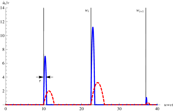
The convergence to the quasi-statics in the small-vv limit occurs on time scales tw:=δ​w/vt_{w}:=\delta w/v where δ​w∼wi+1−wi\delta w\sim w_{i+1}-w_{i} is the typical avalanche separation. twt_{w} is called the waiting time (until the next avalanche). On the other hand, the motion inside an avalanche occurs on the so-called duration time scale

τ∼Lmz≪δ​w/v,\tau\sim L_{m}^{z}\ll\delta w/v\ , (21)

where zz is the dynamical exponent at depinning. In this paper we always assume vv small enough so that the order of scales is as given by Eq. (21), i.e., the avalanche duration is much smaller than the waiting time between avalanches, so that successive avalanches are well separated. In practice, when L≫LmL\gg L_{m} and at least for SR elasticity, it may be sufficient to ask that successive avalanches occurring in the same region of space be well separated, i.e. that (21) holds when δ​w\delta w is the typical separation of avalanches in the same region of space. The condition (21) is equivalent to the condition Lm≪ξvL_{m}\ll\xi_{v}, where ξv\xi_{v} is the correlation length near the depinning transition [43, 44, 45].
Refer to caption
Figure 1: Schematic plot of the instantaneous velocity as a function of v​tvt for different vv. The area under the curve is the avalanche size hence is constant as v→0+v\to 0^{+}. The quasi-static avalanche positions wiw_{i} are indicated.

II.3 Dynamical observables

Our aim is to obtain information about the dynamics in an avalanche. For simplicity we will first consider the nn-times (instantaneous) velocity cumulants u˙t1​…​u˙tn¯c\overline{\dot{u}_{t_{1}}...\dot{u}_{t_{n}}}^{\rm c} for the center of mass, and discuss space dependence later. The important property about avalanches, and non-smooth motion in general, is that in the limit v→0+v\to 0^{+}

u˙t1​…​u˙tn¯c\displaystyle\overline{\dot{u}_{t_{1}}...\dot{u}_{t_{n}}}^{\rm c} =\displaystyle= v​f​(t1,…,tn)+O⁡(v2)\displaystyle vf(t_{1},...,t_{n})+O(v^{2}) (22)
u˙t1​…​u˙tn¯\displaystyle\overline{\dot{u}_{t_{1}}...\dot{u}_{t_{n}}} =\displaystyle= v​f​(t1,…,tn)+O⁡(v2).\displaystyle vf(t_{1},...,t_{n})+O(v^{2})\ . (23)

This means that cumulants and moments are O⁡(v)O(v), and have the same leading time dependence. This is very different from a smooth motion, for which they would be O⁡(vn)O(v^{n}). Here we are considering times much shorter that the waiting-time scale δ​w/v\delta w/v, hence a single avalanche. The result (22) can be understood as follows: The above cumulants are non-negligible only when all times are inside the same avalanche. When that occurs, the velocities are O⁡(v0)O(v^{0}), with a magnitude studied below. Let us suppose that the separation of the times tit_{i} is of the order of TT. The above cumulants are thus dominated by the probability that exactly one avalanche occurs in a time interval of duration TT (with T≪Δ​w/vT\ll\Delta w/v). This probability is in terms of the total avalanche density ρ0\rho_{0}

Prob(one avalanche in[−T/2,T/2])=ρ0vT≪1.\mbox{Prob}(\text{one avalanche in}[-T/2,T/2])=\rho_{0}vT\ll 1\ . (24)

More precisely, one can establish the sum rule

Ln​d∫[−T/2,T/2]ndt1…dtnu˙t1​…​u˙tn¯=ρ0vT⟨Sn⟩+O(v2),L^{nd}\int\limits_{[-T/2,T/2]^{n}}{\mathrm{d}}t_{1}...{\mathrm{d}}t_{n}\,\overline{\dot{u}_{t_{1}}...\dot{u}_{t_{n}}}=\rho_{0}vT\langle S^{n}\rangle+O(v^{2})\ , (25)

which is valid as long as ρ0​v​T≪1\rho_{0}vT\ll 1. It comes from the fact that the total displacement Ld​∫d​t​u˙tL^{d}\int{\mathrm{d}}t\,\dot{u}_{t} during the avalanche ii is equal to its size,

Si=Ld​∫d​t​u˙t.S_{i}=L^{d}\int{\mathrm{d}}t\,\dot{u}_{t}\ . (26)

It is clear from the above that the difference between moments and cumulants is at most of O⁡(v2)O(v^{2}). The sum rule (24) thus connects dynamical quantities to quasi-static ones. It provides a valuable consistency check for our dynamical calculations.

II.4 Strategy

Let us now summarize our strategy. We will calculate the velocity cumulants from perturbation theory in an expansion in the disorder. Naively this expansion is in the bare disorder Δ0​(u)\Delta_{0}(u). To lowest order the nn-times cumulant (22) is O⁡(Δ0n−1)O(\Delta_{0}^{n-1}) and, as we will see below, is obtained from tree graphs in the graphical representation of perturbation theory. For each nn, 1-loop graphs only occur at the next order, i.e. O⁡(Δ0n)O(\Delta_{0}^{n}), and so on for higher-loop graphs. Hence we start by examining the perturbation theory at tree level in the next section. We compute explicitly the lowest moments, and then show that there exists a much more powerful method, based on a simplified field theory, which allows to sum all tree diagrams and compute directly the Laplace transform of the joint probability distribution P⁡(u˙t1,…,u˙tn)P(\dot{u}_{t_{1}},...,\dot{u}_{t_{n}}) of the velocities at nn times.

In practice it is in fact more accurate to work with the renormalized disorder. We recall that the renormalized disorder correlator Δ⁡(u)\Delta(u) is defined in the quasi-static theory from the center-of-mass fluctuations as

m4​[u⁡(w)−w]​[u⁡(w′)−w′]¯c=L−d​Δ​(w−w′).m^{4}\overline{[u(w)-w][u(w^{\prime})-w^{\prime}]}^{\rm c}=L^{-d}\Delta(w-w^{\prime})\ . (27)

The function Δ⁡(u)\Delta(u) depends on mm, with Δ​(u)=Δ0​(u)\Delta(u)=\Delta_{0}(u) for m→∞m\to\infty. At small mm it takes the universal scaling form

Δ⁡(w)\displaystyle\Delta(w) =\displaystyle= 1ϵ​I~2​mϵ−2​ζ​Δ~​(mζ​w),\displaystyle\frac{1}{\epsilon\tilde{I}_{2}}m^{\epsilon-2\zeta}\tilde{\Delta}(m^{\zeta}w)\ , (28)
I~2\displaystyle\tilde{I}_{2} =\displaystyle= ∫q1(q2+1)2.\displaystyle\int_{q}\frac{1}{(q^{2}+1)^{2}}\ . (29)

It is given here for SR elasticity. The rescaled correlator Δ~​(w)\tilde{\Delta}(w) converges to a (non-analytic) fixed-point form Δ~​(w)−−⟶m→0Δ~∗​(w)=O⁡(ϵ)\tilde{\Delta}(w)\stackrel{{\scriptstyle m\to 0}}{{-\!\!\!-\!\!\!\longrightarrow}}\tilde{\Delta}^{*}(w)=O(\epsilon). Here ζ\zeta is the roughness exponent at depinning. The rescaled correlator Δ~​(w)\tilde{\Delta}(w) obeys, as a function of mm, a FRG flow equation which was obtained at the depinning transition, together with its fixed points, to two loops in [41, 48] and checked in [71] where Δ⁡(u)\Delta(u) was measured from numerics.

Since it is the renormalized disorder, which is small, we then reexpress the perturbative expressions of the velocity cumulants in terms of Δ⁡(w)\Delta(w) directly. Thus we generate an expansion in powers of ϵ\epsilon for these quantities. The leading order is determined solely by tree graphs in the renormalized disorder Δ\Delta (each cumulant being of order Δn−1\Delta^{n-1}) and is valid for d=ducd=d_{\rm uc} (to some extent it is also valid for d>ducd>d_{\rm uc}, see the discussion below). This leads to the tree-level result for the velocity probabilities. Corrections to the tree-level result are obtained in the next section by adding the contribution of one-loop diagrams, i.e. the next order in Δ~∗=O⁡(ϵ)\tilde{\Delta}^{*}=O(\epsilon).

In the remainder of the paper we will switch to the comoving frame, unless explicitly indicated. Hence we define for w=v​tw=vt

ux​t=v​t+u˘x​t,u_{xt}=vt+\breve{u}_{xt}\ , (30)

where u˘x​t\breve{u}_{xt} satisfies the equation of motion:

η​∂tu˘x​t=∇x2u˘x​t+F⁡(v​t+u˘x​t,x)−m2​u˘x​t−η​v.\eta\partial_{t}\breve{u}_{xt}=\nabla_{x}^{2}\breve{u}_{xt}+F(vt+\breve{u}_{xt},x)-m^{2}\breve{u}_{xt}-\eta v\ . (31)

Below we will denote u˘\breve{u} by uu for simplicity.

II.5 Expected scaling forms for avalanche statistics

II.5.1 Size distribution

The size distribution is by now the best known one. Let us first recall our previous results [72, 73] for the avalanche-size distribution in the small-mm limit, i.e. Sm≫S0S_{m}\gg S_{0}, where S0S_{0} is the microscopic cutoff, and SmS_{m} the scale of the large avalanches, given by Eq. (20). For S≫S0S\gg S_{0}, the size distribution P⁡(S)P(S) takes the form

Psize​(S)≡P⁡(S)=⟨S⟩Sm2​p​(S/Sm).P_{\rm size}(S)\equiv P(S)=\frac{\langle S\rangle}{S_{m}^{2}}p(S/S_{m})\ . (32)

Depending on the dimension dd, p⁡(s)p(s) takes different forms: (i) for d=ducd=d_{\rm uc}

p(s)=ptree(s)=12​πs−3/2e−s/4.p(s)=p^{\rm tree}(s)=\frac{1}{2\sqrt{\pi}}s^{-3/2}{\mathrm{e}}^{-s/4}\ . (33)

(ii) for d<ducd<d_{\rm uc},

p⁡(s)=A2​π​s−τ​exp⁡(C​s−B4​sδ),p(s)=\frac{A}{2\sqrt{\pi}}s^{-\tau}\exp\!\left(C\sqrt{s}-\frac{B}{4}s^{\delta}\right)\ , (34)

to first order in O⁡(ϵ=duc−d)O(\epsilon=d_{\rm uc}-d), where A−1,B−1,C=O⁡(ϵ)A-1,B-1,C=O(\epsilon) are given in [73]. The exponent δ=1+112​(ϵ−ζ)+O⁡(ϵ2)\delta=1+\frac{1}{12}(\epsilon-\zeta)+O(\epsilon^{2}) and the avalanche exponent

τ=32−18​(ϵ−ζ)+O⁡(ϵ2)\tau=\frac{3}{2}-\frac{1}{8}(\epsilon-\zeta)+O(\epsilon^{2}) (35)

were agree to first order in ϵ\epsilon with the Narayan-Fisher (NF) conjecture [45, 6], which relates the avalanche-size exponent and the roughness exponent via

τ=2−γd+ζ.\tau=2-\frac{\gamma}{d+\zeta}\ . (36)

Here γ=2\gamma=2 for SR elasticity, γ=1\gamma=1 for LR elasticity33 3 The exponent γ\gamma is often called μ\mu in the literature, see e.g. [7]. and duc=2​γd_{\rm uc}=2\gamma. This conjecture agrees well with numerics for d=1,2,3d=1,2,3 [72, 75], both for the statics and quasi-statics (with the respective values for ζ\zeta), but it is not known if it is exact (see the discussion in section VIII-A of [73]). It was proposed by NF for depinning only, but recently we have found a general argument for the statics as well, based on droplet considerations [87, 88].

Here we will recover the above results, within a dynamical calculation, to tree level in d=ducd=d_{\rm uc}, and to one loop, O⁡(ϵ)O(\epsilon), for d<ducd<d_{\rm uc}.

II.5.2 Duration distribution

Assuming one can define unambiguously the duration TT of an avalanche (see the discussion below in Section III.7.3) the duration exponent α\alpha is defined through the small-TT behavior of the duration distribution 44 4 In Section IV the notation α\alpha is used for a different quantity, see Eq. (299). :

Pduration​(T)=1Tα​f​(T/T0),P_{\rm duration}(T)=\frac{1}{T^{\alpha}}f(T/T_{0})\ , (37)

where T0T_{0} is a large-time cutoff, and f⁡(0)f(0) a constant. This form has been conjectured in various articles, see e.g. [6]. A simple scaling argument relates α\alpha to τ\tau and zz, the dynamical exponent. One writes S∼Ld+ζS\sim L^{d+\zeta} and T∼LzT\sim L^{z}, hence S∼T(d+ζ)/zS\sim T^{(d+\zeta)/z}. Then

Pduration​(T)∼Psize​(S∼T(d+ζ)/z)​d​Sd​T∼T−αP_{\rm duration}(T)\sim P_{\rm size}\Big(S\sim T^{(d+\zeta)/z}\Big)\frac{{\mathrm{d}}S}{{\mathrm{d}}T}\sim T^{-\alpha} (38)

with

α=1+(τ−1)​(d+ζ)z.\alpha=1+\frac{(\tau-1)(d+\zeta)}{z}\ . (39)

If we use in addition the NF conjecture (36) one obtains

α=1+d+ζ−γz,\alpha=1+\frac{d+\zeta-\gamma}{z}\ , (40)

a relation which was conjectured previously, see e.g. [6]. It is not known at present whether these conjectures are exact. The methods of the present paper allow to determine Pduration​(T)P_{\rm duration}(T). Here we obtain it to tree level, and in [83] to one loop.

II.5.3 Velocity distribution

Here we obtain the distribution of velocities in an avalanche in the form

𝒫⁡(u˙)∼1u˙a.{\cal P}(\dot{u})\sim\frac{1}{\dot{u}^{a}}\ . (41)

We will obtain a=1a=1 at the mean-field level (tree theory), as in the ABBM model, and a<1a<1 for d<ducd<d_{\rm uc}. It turns out that our result for the exponent aa is not straightforward to derive from scaling arguments. Hence it may be a new independent exponent.

III Tree-level theory

In this section we implement the program explained above to lowest order, i.e. at tree level. Hence we construct the proper mean-field theory for the interface. We will use systematically the notation Δ\Delta for the disorder vertices and η\eta for the friction. Hence, if one substitutes Δ0\Delta_{0} and η0\eta_{0} one gets the naive perturbation result, i.e. genuine tree graphs. If one considers Δ\Delta and η\eta as the renormalized disorder correlator and friction, one obtains the result using the so-called “improved action”, i.e. the limit for d=ducd=d_{\rm uc} of the effective action (see Refs. [73, 74] for more details on these definitions). This amounts to summing tree graphs plus those loop diagrams which renormalize friction or disorder at d=ducd=d_{\rm uc}. Sometimes we will denote Δ→Δm\Delta\to\Delta_{m} and η→ηm\eta\to\eta_{m} to remind that these quantities are mm dependent. In simple terms, the results expressed in terms of Δm\Delta_{m} and ηm\eta_{m} are numerically accurate at d=ducd=d_{\rm uc}, with the correct, and universal, dependence on mm for small mm.

It is useful to recall here the result of [73] for the generating function and avalanche-size distribution at tree level,

ZS​(λ)\displaystyle Z_{S}(\lambda) :⁣=\displaystyle:= ⟨eλ​S−1⟩⟨S⟩,\displaystyle\frac{\left<{\mathrm{e}}^{\lambda S}-1\right>}{\left<S\right>}\ , (42)
ZStree​(λ)\displaystyle Z_{S}^{\mathrm{\rm tree}}(\lambda) =\displaystyle= 12​Sm​(1−1−4​λ​Sm).\displaystyle\frac{1}{2S_{m}}\left(1-\sqrt{1-4\lambda S_{m}}\right)\ . (43)

We have added the subscript SS to distinguish from the notation for the dynamical generating functions introduced below; let us also note that we use indistinguishably the three suffixes “tree”, “MF”, and “00”, to indicate tree, i.e. mean-field quantities. Eq. (43) holds both for the statics and quasi-statics, and will be recovered below in the dynamical approach.

III.1 Calculation of moments

The equation of motion (31) in the comoving frame can also be written as

ux​t=∫x′​t′Rx​t,x′​t′​[F⁡(v​t+ux′​t′,x′)−η​v],u_{xt}=\int_{x^{\prime}t^{\prime}}R_{xt,x^{\prime}t^{\prime}}\Big[F(vt+u_{x^{\prime}t^{\prime}},x^{\prime})-\eta v\Big]\ , (44)

where

Rx​t,x′​t′=Rx−x′,t−t′=(η​∂tδt​t′+gx​x′−1​δt​t′)x​t,x​t′−1R_{xt,x^{\prime}t^{\prime}}=R_{x-x^{\prime},t-t^{\prime}}=\big(\eta\partial_{t}\delta_{tt^{\prime}}+g^{-1}_{xx^{\prime}}\delta_{tt^{\prime}}\big)_{xt,xt^{\prime}}^{-1} (45)

is the bare response function with Rx​t=∫qei​q​x​Rq​tR_{xt}=\int_{q}e^{iqx}R_{qt}. In Fourier space it reads

Rq​t=1ηθ(t)e−(q2+m2)t/η.R_{qt}=\frac{1}{\eta}\theta(t)e^{-(q^{2}+m^{2})t/\eta}\ . (46)

III.1.1 First moment

We start with the first moment, which defines the critical force fc=fc​(m,v)f_{c}=f_{c}(m,v). Taking the disorder average of (44) we have

m2​ux​t¯=fc−η​v\displaystyle m^{2}\overline{u_{xt}}=f_{c}-\eta v (47)
fc:=F⁡(v​t+ux​t,x)¯.\displaystyle f_{c}:=\overline{F(vt+u_{xt},x)\ }\ . (48)

This yields the exact equation

ux​t−ux​t¯=∫x′​t′Rx−x′,t−t′​[F⁡(v​t+ux′​t′,x′)−fc],u_{xt}-\overline{u_{xt}}=\int_{x^{\prime}t^{\prime}}R_{x-x^{\prime},t-t^{\prime}}\big[F(vt+u_{x^{\prime}t^{\prime}},x^{\prime})-f_{c}\big]\ , (49)

from which we now compute the cumulants to leading order in perturbation theory.

III.1.2 Second moment

To lowest order in Δ\Delta one finds from Eq. (49) that

ux1​t1​ux2​t2¯c=∫x′​t′​t′′Rx1−x′,t1−t′​Rx2−x′,t2−t′′​Δ​(v⁡(t′−t′′)).\overline{u_{x_{1}t_{1}}u_{x_{2}t_{2}}}^{\rm c}=\int_{x^{\prime}t^{\prime}t^{\prime\prime}}R_{x_{1}-x^{\prime},t_{1}-t^{\prime}}R_{x_{2}-x^{\prime},t_{2}-t^{\prime\prime}}\Delta\big(v(t^{\prime}-t^{\prime\prime})\big). (50)

From this we obtain the cumulant of the center-of-mass velocity,

u˙t1​u˙t2¯c=L−d​∂t1∂t21η2\displaystyle\overline{\dot{u}_{t_{1}}\dot{u}_{t_{2}}}^{\rm c}=L^{-d}\partial_{t_{1}}\partial_{t_{2}}\frac{1}{\eta^{2}}
×∫s1<t1,s2<t2e−m2η​(t1−s1)−m2η​(t2−s2)​Δ​(v⁡(s1−s2))\displaystyle\times\int_{s_{1}<t_{1},s_{2}<t_{2}}{\mathrm{e}}^{-\frac{m^{2}}{\eta}(t_{1}-s_{1})-\frac{m^{2}}{\eta}(t_{2}-s_{2})}\Delta\big(v(s_{1}-s_{2})\big)
=−L−dv2η2∫τ1>0,τ2>0e−m2η​(τ1+τ2)Δ′′(v(t1−t2−τ1+τ2)).\displaystyle=-L^{-d}\frac{v^{2}}{\eta^{2}}\int\limits_{\tau_{1}>0,\tau_{2}>0}\!\!\!\!\!\!\!{\mathrm{e}}^{-\frac{m^{2}}{\eta}(\tau_{1}+\tau_{2})}\Delta^{\prime\prime}\big(v(t_{1}-t_{2}-\tau_{1}+\tau_{2})\big).

Let us now consider the limit of v→0+v\to 0^{+}, and assume that Δ⁡(u)\Delta(u) has a cusp, i.e.

Δ′′​(u)=2​Δ′​(0+)​δ​(u)+Δ′′​(0)+O⁡(|u|).\Delta^{\prime\prime}(u)=2\Delta^{\prime}(0^{+})\delta(u)+\Delta^{\prime\prime}(0)+O(|u|)\ . (52)

Then we find that

u˙t1​u˙t2¯c\displaystyle\overline{\dot{u}_{t_{1}}\dot{u}_{t_{2}}}^{\rm c} =\displaystyle= −2L−dΔ′(0+)vη2∫τ1>0e−m2η​(2​τ1−t1+t2)\displaystyle-2L^{-d}\Delta^{\prime}(0^{+})\frac{v}{\eta^{2}}\int_{\tau_{1}>0}{\mathrm{e}}^{-\frac{m^{2}}{\eta}(2\tau_{1}-t_{1}+t_{2})} (53)
−L−dv2η2Δ′′(0)∫τ1>0,τ2>0e−m2η​(τ1+τ2)\displaystyle-L^{-d}\frac{v^{2}}{\eta^{2}}\Delta^{\prime\prime}(0)\int\limits_{\tau_{1}>0,\tau_{2}>0}\!\!\!\!{\mathrm{e}}^{-\frac{m^{2}}{\eta}(\tau_{1}+\tau_{2})}
+O⁡(v3).\displaystyle+O(v^{3})\ .

Hence we obtain

u˙t1​u˙t2¯c\displaystyle\overline{\dot{u}_{t_{1}}\dot{u}_{t_{2}}}^{\rm c} =\displaystyle= −L−d​Δ′​(0+)​vm2​η​e−m2η​|t2−t1|\displaystyle-L^{-d}\Delta^{\prime}(0^{+})\frac{v}{m^{2}\eta}{\mathrm{e}}^{-\frac{m^{2}}{\eta}|t_{2}-t_{1}|} (54)
−L−d​Δ′′​(0)​v2m4+O⁡(v3).\displaystyle-L^{-d}\Delta^{\prime\prime}(0)\frac{v^{2}}{m^{4}}+O(v^{3})\ .

Note that the cusp is crucial to get non-smooth, avalanche motion: Since u˙¯=v\overline{\dot{u}}=v, the term of order vv in the above equation is possible only since the manifold moves with velocity u˙\dot{u} of order one (i.e. independent of vv) for a time of order 1/v1/v. In the absence of a cusp, u˙∼v\dot{u}\sim v, and the second cumulant of the velocity is O⁡(v2)O(v^{2}) indicating a smooth motion. To this order, the typical time scale τm\tau_{m} of an avalanche is read off from the exponential in the first line of Eq. (54), as

τm=ηm2.\tau_{m}=\frac{\eta}{m^{2}}\ . (55)

In the improved action, η\eta will be renormalized to η≡ηm\eta\equiv\eta_{m}, as is discussed below.

Using that the size of an avalanche is S=Ld​∫tu˙tS=L^{d}\int_{t}\dot{u}_{t}, we can now integrate over the time difference to obtain

ρ0​v​⟨S2⟩≡L2​d​∫−∞∞d​t​u˙0​u˙t¯c=−2​v​Ld​Δ′​(0+)m4.\rho_{0}v\langle S^{2}\rangle\equiv L^{2d}\int_{-\infty}^{\infty}{\mathrm{d}}t~\overline{\dot{u}_{0}\dot{u}_{t}}^{\rm c}=-2vL^{d}\frac{\Delta^{\prime}(0^{+})}{m^{4}}\ . (56)

Using Eq. (19), i.e. ρ0=Ld/⟨S⟩\rho_{0}=L^{d}/\left<S\right>, this exact relation agrees with the general sum rule for n=2n=2, provided Eq. (20) holds. This is indeed an exact relation obtained both in the statics and in the quasi-static limit in [82, 73]; it relates the cusp to the second moment of the avalanche-size distribution.

In order to simplify the notations for the calculation of higher cumulants, we now switch to dimensionless units. They amount to replacing

x→x/m,L→L/m,t→t​τm,v→v/τmx\to x/m,\quad L\to L/m,\quad t\to t\tau_{m},\quad v\to v/\tau_{m} (57)

and Δ′​(0+)→m4−d​Δ′​(0+)\Delta^{\prime}(0^{+})\to m^{4-d}\Delta^{\prime}(0^{+}). In effect this is equivalent to setting η=m2=1\eta=m^{2}=1.

We now reproduce the above result, introducing a graphical representation which will be useful for the calculation of the higher cumulants. Let us consider Eq. (50) integrated over space and rewrite it graphically as

Ld​ut1​ut2¯c=s1t1​[Uncaptioned image]​s2t2.L^{d}\overline{u_{t_{1}}u_{t_{2}}}^{\rm c}=\rule[-5.69054pt]{0.0pt}{19.91692pt}^{t_{1}}_{s_{1}}\!\!\parbox{37.24228pt}{\hskip 3.44444pt\includegraphics[scale={0.35}]{./figures/cumul2d}\hskip 3.44444pt}\!\rule[-5.69054pt]{0.0pt}{19.91692pt}^{t_{2}}_{s_{2}}\ . (58)

Here the dashed line represents the disorder vertex Δ\Delta which is bilocal in time and the full lines are response functions (46), here taken at zero momentum q=0q=0. (For details on this standard graphical representation see e.g. [48].) The second velocity cumulant thus reads

Ld​u˙t1​u˙t2¯c=∂t1∂t2s1t1​[Uncaptioned image]​s2t2.\!\!\!L^{d}\overline{\dot{u}_{t_{1}}\dot{u}_{t_{2}}}^{\rm c}=\partial_{t_{1}}\partial_{t_{2}}\rule[-5.69054pt]{0.0pt}{19.91692pt}^{t_{1}}_{s_{1}}\!\!\parbox{37.24228pt}{\hskip 3.44444pt\includegraphics[scale={0.35}]{./figures/cumul2d}\hskip 3.44444pt}\!\rule[-5.69054pt]{0.0pt}{19.91692pt}^{t_{2}}_{s_{2}}\ . (59)

Hence the time derivatives act on the external legs. We now use the fact that the response function depends only on the time difference, i.e.,

∂t1Rq,t1−s1=−∂s1Rq,t1−s1,\partial_{t_{1}}R_{q,t_{1}-s_{1}}=-\partial_{s_{1}}R_{q,t_{1}-s_{1}}\ , (60)

where here and below we denote Rt:=Rq=0,t=θ⁡(t)​e−tR_{t}:=R_{q=0,t}=\theta(t)e^{-t} in our dimensionless units. Hence, by partial integration, we can move both time derivatives to act on the disorder vertex as ∂s1∂s2\partial_{s_{1}}\partial_{s_{2}} which produces the term −v2​Δ′′​(v⁡(s1−s2))-v^{2}\Delta^{\prime\prime}(v(s_{1}-s_{2})) as in Eq. (53). To lowest order in vv this can be replaced by −2​v​Δ′​(0+)​δ​(s1−s2)-2v\Delta^{\prime}(0^{+})\delta(s_{1}-s_{2}), hence the two internal times are identified. This can be represented as

Ld​u˙t1​u˙t2¯c=−2​v​Δ′​(0+)​[Uncaptioned image]\displaystyle\!\!\!L^{d}\overline{\dot{u}_{t_{1}}\dot{u}_{t_{2}}}^{\rm c}=-2v\Delta^{\prime}(0^{+})\parbox{32.90608pt}{\hskip 3.44444pt\includegraphics[scale={0.35}]{./figures/cumul2-sum}\hskip 3.44444pt}
=−2vΔ′(0+)∫s1<min⁡(t1,t2)e−(2​s1−t1−t2)\displaystyle=-2v\Delta^{\prime}(0^{+})\int_{s_{1}<\min(t_{1},t_{2})}e^{-(2s_{1}-t_{1}-t_{2})}
=−v​Δ′​(0+)​e−|t1−t2|,\displaystyle=-v\Delta^{\prime}(0^{+})\,{\mathrm{e}}^{-|t_{1}-t_{2}|}\ , (61)

recovering the above result (54) to lowest order in vv.

III.1.3 Third moment

We are now ready to compute the third cumulant. Here and below we label external times by tit_{i} and internal times by sis_{i} (black dots). To lowest order in the disorder, one finds from Eq. (49):

L2​d​u˙t1​u˙t2​u˙t3¯c=∂t1∂t2∂t3[6​Sym  [Uncaptioned image]  ]L^{2d}\overline{\dot{u}_{t_{1}}\dot{u}_{t_{2}}\dot{u}_{t_{3}}}^{\rm c}=\partial_{t_{1}}\partial_{t_{2}}\partial_{t_{3}}\left[6\,\mbox{Sym}\parbox{71.20918pt}{\hskip 3.44444pt\includegraphics[scale={0.35}]{./figures/cumul3d}\hskip 3.44444pt}\right] (62)

where Sym{\rm Sym} denotes symmetrization w.r.t. the external times tit_{i}. Hence one has

L2​d​u˙t1​u˙t2​u˙t3¯=6​Sym​∂t1∂t2∂t3[Uncaptioned image],.L^{2d}\overline{\dot{{u}}_{t_{1}}\dot{{u}}_{t_{2}}\dot{{u}}_{t_{3}}}=6\,\mbox{Sym}\,\partial_{t_{1}}\partial_{t_{2}}\partial_{t_{3}}\parbox{71.20918pt}{\hskip 3.44444pt\includegraphics[scale={0.35}]{./figures/cumul3d}\hskip 3.44444pt}\ ,\ . (63)

The first thing one could do is to perform the ∂t3\partial_{t_{3}} derivative, using partial integrations

∫s4∂t3Rt3−s4​Δ′​(s3−s4)\displaystyle\int_{s_{4}}\partial_{t_{3}}R_{t_{3}-s_{4}}\Delta^{\prime}(s_{3}-s_{4})
=−∫s4∂s4Rt3−s4Δ′(s3−s4)\displaystyle\qquad=-\int_{s_{4}}\partial_{s_{4}}R_{t_{3}-s_{4}}\Delta^{\prime}(s_{3}-s_{4})
=∫s4Rt3−s4​∂s4Δ′​(s3−s4)\displaystyle\qquad=\int_{s_{4}}R_{t_{3}-s_{4}}\partial_{s_{4}}\Delta^{\prime}(s_{3}-s_{4})
=−2Δ′(0+)∫s4Rt3−s4δ(s3−s4).\displaystyle\qquad=-2\Delta^{\prime}(0^{+})\int_{s_{4}}R_{t_{3}-s_{4}}\delta(s_{3}-s_{4})\ .~~~ (64)

Note that we have safely replaced Δ′​(v⁡(s3−s4))\Delta^{\prime}(v(s_{3}-s_{4})) by Δ′​(s3−s4)\Delta^{\prime}(s_{3}-s_{4}) since we anticipate that to lowest order we will need only Δ′​(u)=Δ′​(0+)​sgn​(u)+O⁡(u)\Delta^{\prime}(u)=\Delta^{\prime}(0^{+}){\rm sgn}(u)+O(u). Note that there is no boundary term if time integrals are performed from [−∞,∞][-\infty,\infty] and the theta function is included in RR. By this procedure, the term Δ⁡(s3−s4)\Delta(s_{3}-s_{4}) will have exactly two derivatives. However, to be able to proceed further, it is better to consider ∂t2∂t3\partial_{t_{2}}\partial_{t_{3}} simultaneously, while symmetrizing at the same time leading instead to (passing always one external derivative onto each disorder vertex-end):

12​∂t2∂t3[[Uncaptioned image]+[Uncaptioned image]]\displaystyle\!\!\!\frac{1}{2}\partial_{t_{2}}\partial_{t_{3}}\left[\parbox{43.02388pt}{\hskip 3.44444pt\includegraphics[scale={0.35}]{./figures/cumul-brick1}\hskip 3.44444pt}+\parbox{43.02388pt}{\hskip 3.44444pt\includegraphics[scale={0.35}]{./figures/cumul-brick2}\hskip 3.44444pt}\right] (65)
=\displaystyle= −Δ′(0+)∫s4[∂t2R(t2−s3)R(t3−s4)δ(s3−s4)\displaystyle-\Delta^{\prime}(0^{+})\int_{s_{4}}\Big[\partial_{t_{2}}R(t_{2}-s_{3})R(t_{3}-s_{4})\delta(s_{3}-s_{4})
+R(t2−s4)∂t3R(t3−s3)δ(s3−s4)]\displaystyle~~~~~~~~~~~~~~~~~~~~~~~+R(t_{2}-s_{4})\partial_{t_{3}}R(t_{3}-s_{3})\delta(s_{3}-s_{4})\Big]
=\displaystyle= −Δ′(0+)(∂t2+∂t3)[R(t2−s3)R(t3−s3)]\displaystyle-\Delta^{\prime}(0^{+})\left(\partial_{t_{2}}+\partial_{t_{3}}\right)\Big[R(t_{2}-s_{3})R(t_{3}-s_{3})\Big]
=\displaystyle= Δ′​(0+)​∂s3[R⁡(t2−s3)​R​(t3−s3)].\displaystyle\Delta^{\prime}(0^{+})\partial_{s_{3}}\Big[R(t_{2}-s_{3})R(t_{3}-s_{3})\Big]\ .

Integration by part w.r.t. s3s_{3} is then possible, and together with taking ∂t1\partial_{t_{1}} on the left branch and using time translational invariance of Rs3−s2R_{s_{3}-s_{2}} and Rt1−s1R_{t_{1}-s_{1}} respectively leads to two derivatives on the lower vertex Δ⁡(s1−s2)\Delta(s_{1}-s_{2}).

In summary, we find that the surplus external derivatives can always be passed down in the tree, so that at the end each vertex receives exactly two derivatives. This means that we can rewrite (63) as

L2​d​u˙t1​u˙t2​u˙t3¯=6​v​Δ′​(0+)2​Sym​∫s1∫s2[Uncaptioned image],L^{2d}\overline{\dot{{u}}_{t_{1}}\dot{{u}}_{t_{2}}\dot{{u}}_{t_{3}}}=6v\Delta^{\prime}(0^{+})^{2}\,\mbox{Sym}\,\int_{s_{1}}\int_{s_{2}}\parbox{50.97359pt}{\hskip 3.44444pt\includegraphics[scale={0.35}]{./figures/cumul3-sum}\hskip 3.44444pt}\ , (66)

where the points are intermediate times, and the arrows standard response functions. We now have to compute this new diagram, with the huge simplification that vertices are now local in time and which apart from the vertices contains only response functions.

We also note that the single vv factor comes from the lower vertex: This can be interpreted as the point in space and time, where an avalanche is triggered with rate vv.

Let us now complete the integration over internal times. To this aim, let us fix the smallest internal time s1s_{1}, and integrate over s2s_{2}:

∫s2[Uncaptioned image]=Rt1−s1​∫s2Rt2−s2​Rt3−s2​Rs2−s1\displaystyle\int_{s_{2}}\parbox{50.97359pt}{\hskip 3.44444pt\includegraphics[scale={0.35}]{./figures/cumul3-sum}\hskip 3.44444pt}=R_{t_{1}-s_{1}}\int_{s_{2}}R_{t_{2}-s_{2}}R_{t_{3}-s_{2}}R_{s_{2}-s_{1}} (67)
=\displaystyle= Rt1−s1​[e−[max⁡(t2,t3)−s1]−e−(t2−s1)−(t3−s1)]\displaystyle R_{t_{1}-s_{1}}\left[{\mathrm{e}}^{-[\max(t_{2},t_{3})-s_{1}]}-{\mathrm{e}}^{-(t_{2}-s_{1})-(t_{3}-s_{1})}\right]
×Θ⁡(s1<min⁡(t2,t3)).\displaystyle\times\Theta(s_{1}<\min(t_{2},t_{3}))\ .

Integrating once more gives

∫s1,s2[Uncaptioned image]\displaystyle\int_{s_{1},s_{2}}\parbox{50.97359pt}{\hskip 3.44444pt\includegraphics[scale={0.35}]{./figures/cumul3-sum}\hskip 3.44444pt} =\displaystyle= 12​e2​min⁡(t1,t2,t3)−t1−max⁡(t2,t3)\displaystyle\frac{1}{2}{\mathrm{e}}^{2\min(t_{1},t_{2},t_{3})-t_{1}-\max(t_{2},t_{3})} (68)
−\displaystyle- 13​e3​min⁡(t1,t2,t3)−t1−t2−t3.\displaystyle\frac{1}{3}{\mathrm{e}}^{3\min(t_{1},t_{2},t_{3})-t_{1}-t_{2}-t_{3}}\ .

Finally, after symmetrization it simplifies into

6​Sym​∫s1,s2[Uncaptioned image]\displaystyle\!\!\!6\,\mbox{Sym}\int_{s_{1},s_{2}}\parbox{50.97359pt}{\hskip 3.44444pt\includegraphics[scale={0.35}]{./figures/cumul3-sum}\hskip 3.44444pt}
=emin⁡(t1,t2,t3)−max⁡(t1,t2,t3).\displaystyle={\mathrm{e}}^{\min(t_{1},t_{2},t_{3})-\max(t_{1},t_{2},t_{3})}\ . (69)

Hence, assuming that the external times are ordered as t1<t2<t3t_{1}<t_{2}<t_{3} we obtain our final result for the third velocity cumulant as

L2​d​u˙t1​u˙t2​u˙t3¯c\displaystyle L^{2d}\overline{\dot{{u}}_{t_{1}}\dot{{u}}_{t_{2}}\dot{{u}}_{t_{3}}}^{\rm c} =\displaystyle= 2​v​Δ′​(0+)2​et1−t3\displaystyle 2v\Delta^{\prime}(0^{+})^{2}{\mathrm{e}}^{t_{1}-t_{3}} (70)
=\displaystyle= 2vΔ′(0+)2e−(|t1−t2|+|t1−t3|+|t2−t3|)/2.\displaystyle 2v\Delta^{\prime}(0^{+})^{2}{\mathrm{e}}^{-(|t_{1}-t_{2}|+|t_{1}-t_{3}|+|t_{2}-t_{3}|)/2}\ .\quad

Note that the final expression is simple, while the starting one was quite non-trivial.

We can now check that the sum rule (25) is satisfied. Indeed

v​⟨S3⟩⟨S⟩\displaystyle v\frac{\langle S^{3}\rangle}{\langle S\rangle} =\displaystyle= L2​d​∫t2∫t3u˙t1​u˙t2​u˙t3¯c\displaystyle L^{2d}\int_{t_{2}}\int_{t_{3}}\overline{\dot{{u}}_{t_{1}}\dot{{u}}_{t_{2}}\dot{{u}}_{t_{3}}}^{\rm c} (71)
=\displaystyle= 12​v​Δ′​(0+)2​∫0=t1<t2<t3et1−t3\displaystyle 12\,v\Delta^{\prime}(0^{+})^{2}\int_{0=t_{1}<t_{2}<t_{3}}{\mathrm{e}}^{t_{1}-t_{3}}~~~~~~~~
=\displaystyle= 12​v​Δ′​(0+)2\displaystyle 12v\Delta^{\prime}(0^{+})^{2}

recovering the result of [73], and which can be obtained by expanding (43) for the third moment of the avalanche-size distribution.

III.1.4 Fourth moment

The higher moments can be computed using the same method, as the same simplifying features can be generalized. The result for the fourth cumulant is, supposing the times are ordered as t1<t2<t3<t4t_{1}<t_{2}<t_{3}<t_{4}:

L3​d​u˙t1​u˙t2​u˙t3​u˙t4¯\displaystyle L^{3d}\overline{\dot{{u}}_{t_{1}}\dot{{u}}_{t_{2}}\dot{{u}}_{t_{3}}\dot{{u}}_{t_{4}}} (73)
=\displaystyle= −24vΔ′(0+)3Sym[[Uncaptioned image]\displaystyle-24v\Delta^{\prime}(0^{+})^{3}\,\mbox{Sym}\left[\parbox{68.31839pt}{\hskip 3.44444pt\includegraphics[scale={0.35}]{./figures/cumul4-sum-2}\hskip 3.44444pt}\right.
= - 24 v Δ’(0^+)^3 Sym+4[Uncaptioned image]]\displaystyle\hphantom{= - 24 v \Delta'(0^+)^3 \,\mbox{Sym}}+4\left.\parbox{69.04109pt}{\hskip 3.44444pt\includegraphics[scale={0.35}]{./figures/cumul4-sum-1}\hskip 3.44444pt}\right]
=v​|Δ′​(0+)|3​[4​et1−t4+2​et1+t2−t3−t4]\displaystyle=v|\Delta^{\prime}(0^{+})|^{3}[4{\mathrm{e}}^{t_{1}-t_{4}}+2{\mathrm{e}}^{t_{1}+t_{2}-t_{3}-t_{4}}]

The sum rule gives

v​⟨S4⟩⟨S⟩=L3​d​∫t2,t3,t4u˙t1​u˙t2​u˙t3​u˙t4¯=120​v​|Δ′​(0+)|3,v\frac{\langle S^{4}\rangle}{\langle S\rangle}=L^{3d}\int_{t_{2},t_{3},t_{4}}\overline{\dot{{u}}_{t_{1}}\dot{{u}}_{t_{2}}\dot{{u}}_{t_{3}}\dot{{u}}_{t_{4}}}=120v|\Delta^{\prime}(0^{+})|^{3}\ , (74)

which coincides with the result for the fourth moment of Eq. (43).

III.1.5 Fifth moment

Finally, we give the fifth moment

L4​d​u˙t1​u˙t2​u˙t3​u˙t4​u˙t5¯\displaystyle L^{4d}\overline{\dot{{u}}_{t_{1}}\dot{{u}}_{t_{2}}\dot{{u}}_{t_{3}}\dot{{u}}_{t_{4}}\dot{{u}}_{t_{5}}}
=v​Δ′​(0+)4​5!​Sym​[8​[Uncaptioned image]+2​[Uncaptioned image]+4​[Uncaptioned image]]\displaystyle=v\Delta^{\prime}(0^{+})^{4}5!\,\mbox{Sym}\left[8\parbox{87.10858pt}{\hskip 3.44444pt\includegraphics[scale={0.35}]{./figures/cumul5-sum-2}\hskip 3.44444pt}+2\parbox{87.10858pt}{\hskip 3.44444pt\includegraphics[scale={0.35}]{./figures/cumul5-sum-1}\hskip 3.44444pt}+4\parbox{87.10858pt}{\hskip 3.44444pt\includegraphics[scale={0.35}]{./figures/cumul5-sum-3}\hskip 3.44444pt}\right]
=v​Δ′​(0+)4​[8​et1−t4+4​et1+t2−t3−t5+8​et1+t2−t4−t5+4​et1+t3−t4−t5]\displaystyle=v\Delta^{\prime}(0^{+})^{4}[8{\mathrm{e}}^{t_{1}-t_{4}}+4{\mathrm{e}}^{t_{1}+t_{2}-t_{3}-t_{5}}+8{\mathrm{e}}^{t_{1}+t_{2}-t_{4}-t_{5}}+4{\mathrm{e}}^{t_{1}+t_{3}-t_{4}-t_{5}}] (75)

We check that

v​⟨S4⟩⟨S⟩=L4​d​∫t2,t3,t4,t5u˙t1​u˙t2​u˙t3​u˙t4​u˙t5¯=5!×14​v​Δ′​(0+)4v\frac{\langle S^{4}\rangle}{\langle S\rangle}=L^{4d}\int_{t_{2},t_{3},t_{4},t_{5}}\overline{\dot{{u}}_{t_{1}}\dot{{u}}_{t_{2}}\dot{{u}}_{t_{3}}\dot{{u}}_{t_{4}}\dot{{u}}_{t_{5}}}=5!\times 14v\Delta^{\prime}(0^{+})^{4} (76)

coincides with the result for the fifth moment of (43).

The above results suggest that there is an underlying simplification at the level of tree diagrams of the original field theory, which is non-local in time, into a field theory which is local in time. We now show how the latter arises.

III.2 Generating function and instanton equation: Simplified (tree) field theory

Since here we want to study the temporal and spatial statistics of the instantaneous velocity field, we define the following generating functional of a (possibly space- and time-dependent) source field λx​t\lambda_{xt},

G⁡[λ]:=e∫tλx​t​(v+u˙x​t)¯.G[\lambda]:=\overline{{\mathrm{e}}^{\int_{t}\lambda_{xt}(v+\dot{u}_{xt})}}\ . (77)

We remind that we are working in the comoving frame, i.e. v+u˙x​tv+\dot{u}_{xt} is the velocity of the manifold in the laboratory frame. The functional G⁡[λ]G[\lambda] encodes all possible information. In particular, all moments can be recovered by differentiation w.r.t. the source. In this article we focus on the small driving-velocity limit. In view of the results of the previous sections, it will be sufficient to compute the generating function,

Z⁡[λ]:=L−d​∂vG⁡[λ]|v=0+,Z[\lambda]:=L^{-d}\partial_{v}G[\lambda]\Big|_{v=0^{+}}\ , (78)

which contains the leading O⁡(v)O(v) dependence of all moments in the limit of small velocity v=0+v=0^{+}.

It turns out that, within the tree level theory, it is possible to compute these generating functions and obtain all cumulants at once, as well as the velocity distribution. We now show how this simplification occurs.

We start not from the equation of motion (1), but from its time derivative in the comoving frame55 5 Below, when indicated, we will alternatively use this equation in the laboratory frame, which amounts to setting v=0v=0 in Eq. (79).

(η∂t−∇x2+m2)u˙x​t=∂tF(vt+ux​t,x)+f˙x​t−m2v.(\eta\partial_{t}-\nabla^{2}_{x}+m^{2})\dot{u}_{xt}=\partial_{t}F(vt+u_{xt},x)+\dot{f}_{xt}-m^{2}v\ . (79)

For completeness we wrote it for arbitrary driving fx​t=(m2−∇x2)​wx​tf_{xt}=(m^{2}-\nabla^{2}_{x})w_{xt}, however we will mostly specialize to uniform driving, i.e. w˙x​t=v\dot{w}_{xt}=v, f˙x​t=m2​v\dot{f}_{xt}=m^{2}v, in which case the last term is zero. We denote indifferently time derivatives by u˙\dot{u} or ∂tu\partial_{t}u, and for now we use the original (microscopic) units. Again, one has to set η→η0\eta\to\eta_{0}, Δ→Δ0\Delta\to\Delta_{0} for a derivation starting from the bare model, or the renormalized parameters if one deals with the improved action.

We now average over disorder (and initial conditions) using the MSR dynamical action SS associated to the equation of motion (79):

𝒮\displaystyle{\cal S} =\displaystyle= 𝒮0+𝒮dis\displaystyle{\cal S}_{0}+{\cal S}_{\mathrm{dis}} (80)
𝒮0\displaystyle{\cal S}_{0} =\displaystyle= ∫x​tu~x​t(η∂t−∇x2+m2)u˙x​t\displaystyle\int_{xt}\tilde{u}_{xt}(\eta\partial_{t}-\nabla_{x}^{2}+m^{2})\dot{u}_{xt} (81)
𝒮dis\displaystyle{\cal S}_{\rm dis} =\displaystyle= −12∫x​t​t′u~x​tu~x​t′∂t∂t′Δ(v(t−t′)+ux​t−ux​t′).\displaystyle-\frac{1}{2}\int_{xtt^{\prime}}\tilde{u}_{xt}\tilde{u}_{xt^{\prime}}\partial_{t}\partial_{t^{\prime}}\Delta\big(v(t{-}t^{\prime})+u_{xt}{-}u_{xt^{\prime}}\big).~~~~~~~~~ (82)

Note that this is the dynamical action associated to the velocity theory, i.e. in terms of u~x​t\tilde{u}_{xt} and u˙x​t\dot{u}_{xt} to be distinguished from the one usually considered, associated to the position theory, in terms of u^x​t\hat{u}_{xt} and ux​tu_{xt}, to be discussed below.

The generating function (77) can then be written as

G⁡[λ]\displaystyle G[\lambda] =\displaystyle= ∫𝒟⁡[u˙]​𝒟​[u~]​e−𝒮λ\displaystyle\int{\cal D}[\dot{u}]{\cal D}[\tilde{u}]e^{-{\cal S}_{\lambda}} (83)
𝒮λ\displaystyle{\cal S}_{\lambda} =\displaystyle= 𝒮−∫x​tλx​t​(v+u˙x​t),\displaystyle{\cal S}-\int_{xt}\lambda_{xt}(v+\dot{u}_{xt})\ , (84)

with G⁡[0]=1G[0]=1 and Z⁡[0]=0,Z[0]=0, since the dynamical partition function is normalized to unity. We can rewrite for the time-derivatives appearing in Eq. (82)

∂t∂t′Δ⁡(v⁡(t−t′)+ux​t−ux​t′)\displaystyle\partial_{t}\partial_{t^{\prime}}\Delta(v(t-t^{\prime})+u_{xt}-u_{xt^{\prime}}) (85)
=(v+u˙x​t)​∂t′Δ′​(v⁡(t−t′)+ux​t−ux​t′)\displaystyle=(v+\dot{u}_{xt})\partial_{t^{\prime}}\Delta^{\prime}(v(t-t^{\prime})+u_{xt}-u_{xt^{\prime}})
=(v+u˙x​t)​Δ′​(0+)​∂t′sgn⁡(t−t′)+….\displaystyle=(v+\dot{u}_{xt})\Delta^{\prime}(0^{+})\partial_{t^{\prime}}{\rm sgn}(t-t^{\prime})+...\ .

Here we have used that sgn⁡(v⁡(t−t′)+ux​t−ux​t′)=sgn⁡(t−t′){\rm sgn}(v(t-t^{\prime})+u_{xt}-u_{xt^{\prime}})={\rm sgn}(t-t^{\prime}), i.e. the motion for v>0v>0 is monotonously forward, as guaranteed by the Middleton theorem [68]. The neglected terms in Eq. (85) are higher derivatives of Δ⁡(u)|u=0+\Delta(u)|_{u=0^{+}}. As we discuss below at length, they contribute only to O⁡(ϵ=4−d)O(\epsilon=4-d) to Z⁡[λ],Z[\lambda], hence they can be neglected at tree level. This is consistent with our findings in the previous section that only Δ′​(0+)\Delta^{\prime}(0^{+}) appears at tree level. Hence we can rewrite the disorder part 𝒮dis{\cal S}_{\mathrm{dis}} of the dynamical action, which is a priori non-local in time, as 𝒮dis=𝒮distree+…{\cal S}_{\mathrm{dis}}={\cal S}^{\mathrm{tree}}_{\mathrm{dis}}+..., where

𝒮distree=Δ′​(0+)​∫x​tu~x​t​u~x​t​(v+u˙x​t){\cal S}^{\mathrm{tree}}_{\mathrm{dis}}=\Delta^{\prime}(0^{+})\int_{xt}\tilde{u}_{xt}\tilde{u}_{xt}(v+\dot{u}_{xt}) (86)

is an action local in time. Furthermore we recognize the cubic vertex which generates the simple graphs obtained in the previous sections by a systematic perturbation expansion. The action

𝒮tree:=𝒮0+𝒮distree{\cal S}^{\mathrm{tree}}:={\cal S}_{0}+{\cal S}_{\mathrm{dis}}^{\mathrm{tree}} (87)

is the so-called tree-level, or mean-field, action. Note that if we use the improved action, it then includes the loop corrections to η\eta and Δ\Delta, and yields the correct result for d=duc=4d=d_{\rm uc}=4, making the dependence in mm explicit as η→ηm\eta\to\eta_{m} and Δ→Δm\Delta\to\Delta_{m}, see the discussion below and in Ref. [73]. Note that due to the STS symmetry mentioned above, m2m^{2}, the elastic coefficient in front of ∇2ux​t\nabla^{2}u_{xt}, and vv are not corrected.

We can now study algebraically the tree approximation

Ztree​[λ]\displaystyle Z^{\mathrm{tree}}[\lambda] =\displaystyle= L−d​∂vGtree​[λ]|v=0+\displaystyle L^{-d}\partial_{v}G^{\mathrm{tree}}[\lambda]\Big|_{v=0^{+}} (88)
Gtree​[λ]\displaystyle G^{\mathrm{tree}}[\lambda] =\displaystyle= ∫𝒟⁡[u˙]​𝒟​[u~]​e−𝒮λtree\displaystyle\int{\cal D}[\dot{u}]{\cal D}[\tilde{u}]e^{-{\cal S}^{\mathrm{tree}}_{\lambda}} (89)
𝒮λtree\displaystyle{\cal S}^{\mathrm{tree}}_{\lambda} =\displaystyle= 𝒮tree−∫tλx​t​(v+u˙x​t).\displaystyle{\cal S}^{\mathrm{tree}}-\int_{t}\lambda_{xt}(v+\dot{u}_{xt})\ . (90)

Note that the highly non-linear action (81) (82) has been reduced to a much simpler cubic theory. Cubic theories among others describe branching processes, such as the Reggeon field theory [95] for directed percolation. The present theory however is simpler, and can be reduced to a non-linear equation as we now explain.

Remarkably, considering (88), one notices that u˙x​t\dot{u}_{xt} appears in 𝒮λtree{\cal S}^{\mathrm{tree}}_{\lambda} only linearly, i.e. in the form ∫x​tu˙x​t​Ox​t​[u~,λ]\int_{xt}\dot{u}_{xt}O_{xt}[\tilde{u},\lambda]. It can thus be integrated out, leading to a δ\delta-function constraint66 6 Equivalently one can view u˙x​t\dot{u}_{xt} as a response field associated to the equation Ox​t​[u~,λ]=0.O_{xt}[\tilde{u},\lambda]=0. ∏x​tδ⁡(Ox​t​[u~,λ])\prod_{xt}\delta(O_{xt}[\tilde{u},\lambda]). Hence in the tree-level theory the field u~x​t\tilde{u}_{xt} is not fluctuating, but given by the non-linear equation

(η∂t+∇x2−m2)u~x​t−Δ′(0+)u~x​t2+λx​t=0.(\eta\partial_{t}+\nabla_{x}^{2}-m^{2})\tilde{u}_{xt}-\Delta^{\prime}(0^{+})\tilde{u}_{xt}^{2}+\lambda_{xt}=0\ . (91)

This equation is the saddle-point equation w.r.t. u˙\dot{u} of 𝒮λtree{\cal S}^{\mathrm{tree}}_{\lambda} in presence of a source, and is satisfied exactly. We also call it the instanton equation. We denote u~x​tλ\tilde{u}^{\lambda}_{xt} the solution of this equation for a given source field λx​t\lambda_{xt} with u~λ=0=0\tilde{u}^{\lambda=0}=0. After integration over u˙x​t\dot{u}_{xt}, we thus obtain from Eqs. (87) to (90):

G⁡[λ]\displaystyle G[\lambda] =\displaystyle= ev​Ld​Z​[λ]\displaystyle e^{vL^{d}Z[\lambda]} (92)
Z⁡[λ]\displaystyle Z[\lambda] =\displaystyle= L−d​∫x​t[λx​t−Δ′​(0+)​(u~x​tλ)2]\displaystyle L^{-d}\int_{xt}[\lambda_{xt}-\Delta^{\prime}(0^{+})(\tilde{u}_{xt}^{\lambda})^{2}] (93)
=\displaystyle= −L−d∫x​t(η∂t+∇x2−m2)u~x​tλ\displaystyle-L^{-d}\int_{xt}(\eta\partial_{t}+\nabla_{x}^{2}-m^{2})\tilde{u}^{\lambda}_{xt}
=\displaystyle= m2​L−d​∫x​tu~x​tλ.\displaystyle m^{2}L^{-d}\int_{xt}\tilde{u}^{\lambda}_{xt}\ .

Here we have used the saddle-point equation (91) and, in the last equality, assumed that u~x​tλ\tilde{u}_{xt}^{\lambda} (resp. ∇xu~λ\nabla_{x}\tilde{u}^{\lambda}) vanishes at large tt (resp. xx). This is insured if the source vanishes at infinity which we assume in the following. Note that since Z⁡[λ]Z[\lambda] is independent of the velocity, Eq. (92) gives the full dependence at finite vv, a fact which is exploited and studied in detail in Ref. [84].

In summary we find that the calculation of Z⁡[λ]Z[\lambda], i.e. of all cumulants of the velocity field, is equivalent to solving the non-linear equation (91). The solution u~x​tλ\tilde{u}^{\lambda}_{xt} can be constructed perturbatively in an expansion in powers of the source λx​t\lambda_{xt}. To lowest order

u~x′​t′λ=∫x,tλx​t​Rx​t,x′​t′+O⁡(λ2),\tilde{u}^{\lambda}_{x^{\prime}t^{\prime}}=\int_{x,t}\lambda_{xt}R_{xt,x^{\prime}t^{\prime}}+O(\lambda^{2})\ , (94)

where Rx​t,x′​t′R_{xt,x^{\prime}t^{\prime}} is the usual bare response function (45). Integrating Eq. (99) or (94), one finds

Z⁡(λ)=L−d​∫x​tλx​t+O⁡(λ2),Z(\lambda)=L^{-d}\int_{xt}\lambda_{xt}+O(\lambda^{2})\ , (95)

which is consistent with u˙x​t¯=0\overline{\dot{u}_{xt}}=0 (vv is uncorrected). Pursuing to O⁡(λ2)O(\lambda^{2}) and higher orders, one recovers the velocity cumulants obtained in the previous sections, and in addition obtains their full spatial dependence. Instead of working perturbatively, we obtain and analyze in the next subsection the (joint) probability distributions of the velocity at one (and several) times, focusing on the simplest observable, the center-of-mass velocity u˙t\dot{u}_{t}.

Let us note that the simplified (tree) theory defined above does not contain all tree graphs. There are other tree graphs involving Δ′′​(0)\Delta^{\prime\prime}(0) and higher derivatives, as e.g. the following configurations of order v2v^{2},

[Uncaptioned image]+[Uncaptioned image]+[Uncaptioned image].\parbox{43.02388pt}{\hskip 3.44444pt\includegraphics[scale={0.35}]{./figures/cumul-brick4}\hskip 3.44444pt}+\parbox{42.30118pt}{\hskip 3.44444pt\includegraphics[scale={0.35}]{./figures/cumul-brick3}\hskip 3.44444pt}+\parbox{42.30118pt}{\hskip 3.44444pt\includegraphics[scale={0.35}]{./figures/cumul-brick5}\hskip 3.44444pt}. (96)

While they are similar to those in Eq. (58), different classes of trees appear starting at the fourth moment, as e.g.

[Uncaptioned image].\parbox{96.5037pt}{\hskip 3.44444pt\includegraphics[scale={0.35}]{./figures/cumul-brick6}\hskip 3.44444pt}\ . (97)

These diagrams are characterized by the fact that they have two (or more) roots (lowest vertices), and are of order v2v^{2} (or higher). The full tree theory is studied in section V and can be reduced to two non-linear saddle-point equations. However since these additional tree graphs lead to contributions which are of higher order in vv, to study a single avalanche in the small-vv limit, they are not needed.

Finally, it is important to stress that the above simplified tree theory corresponds to the problem of an elastic manifold in a random-force landscape made out of uncorrelated Brownian motions, for which it is exact for monotonous driving. This is the BFM, discussed in Section III.7.

III.3 Joint probability distributions for the center-of-mass velocity

To analyze the results, it is convenient to use dimensionless equations, hence replacing x→x/mx\to x/m, and t→τm​tt\to\tau_{m}t. In mean field τm=η/m2\tau_{m}=\eta/m^{2}, λ→λ​τm/Sm\lambda\to\lambda\tau_{m}/S_{m}, u~x​t→u~x​t/(m2​Sm)\tilde{u}_{xt}\to\tilde{u}_{xt}/(m^{2}S_{m}), and v→v​vmv\to vv_{m}, where vm=Sm​md/τmv_{m}=S_{m}m^{d}/\tau_{m}, L→L/mL\to L/m. We start by using these units and, whenever indicated, switch back to dimension-full units in discussing the final results. We also keep the factor of LdL^{d} in the beginning, but later on we find it convenient to suppress it. That amounts to a further change of units as v→v​v~mv\to v\tilde{v}_{m} with v~m=(m​L)−d​vm\tilde{v}_{m}=(mL)^{-d}v_{m} whenever indicated below.

III.3.1 1-time center-of-mass velocity distribution

The center-of-mass velocity distribution is obtained by choosing a uniform λx​t=λt\lambda_{xt}=\lambda_{t}. The 1-time probability is obtained from the inverse Laplace transform of Z~​(λ)\tilde{Z}(\lambda), choosing λt:=λ​δ​(t)\lambda_{t}:=\lambda\delta(t),

Z~​(λ)=L−d​∂veLd​λ​(v+u˙)¯|v=0+.\tilde{Z}(\lambda)=L^{-d}\partial_{v}\overline{e^{L^{d}\lambda(v+\dot{u})}}|_{v=0^{+}}\ . (98)

Here u˙=u˙t=0\dot{u}=\dot{u}_{t=0}, and the tilde on Z~​(λ)\tilde{Z}(\lambda) reminds us that we use dimensionless units. The saddle-point equation (91) admits a spatially uniform solution u~x​t=u~t\tilde{u}_{xt}=\tilde{u}_{t}, thus we need to solve

(∂t−1)u~t+u~t2=−λδ(t).(\partial_{t}-1)\tilde{u}_{t}+\tilde{u}_{t}^{2}=-\lambda\delta(t)\ . (99)

The boundary condition is u~t→0\tilde{u}_{t}\to 0 at t=±∞t=\pm\infty, leading to

u~t=λλ+(1−λ)​e−t​θ​(−t).\tilde{u}_{t}=\frac{\lambda}{\lambda+(1-\lambda)e^{-t}}\theta(-t)\ . (100)

This gives the generating function

Z~​(λ)=∫tu~t=−ln⁡(1−λ).\tilde{Z}(\lambda)=\int_{t}\tilde{u}_{t}=-\ln(1-\lambda)\ . (101)

We now want to infer from this the 1-time velocity distribution in an avalanche. Before doing so, let us restore dimension-full units. We assume that in the limit v=0+v=0^{+} there are times when the velocity is exactly zero, i.e. v+u˙=0v+\dot{u}=0 (since we use the co-moving frame) and times (when an avalanche is proceeding) when the velocity is non-zero. This picture is confirmed by results below 77 7 This gives the universal regime for u˙≫v0\dot{u}\gg v_{0}. For velocities smaller than the cutoff v0v_{0} one expects a dependence on the details of the dynamics.. Hence the 1-time velocity probability (at say time t=0t=0) must take the form

P⁡(u˙)=(1−pa)​δ​(v+u˙)+pa​𝒫​(u˙).P(\dot{u})=(1-p_{a})\delta(v+\dot{u})+p_{a}{{\cal P}}(\dot{u})\ . (102)

Here pap_{a} is the probability that t=0t=0 belongs to an avalanche, and 𝒫⁡(u˙){{\cal P}}(\dot{u}) is the conditional probability of velocity, given that t=0t=0 belongs to an avalanche. Both 𝒫{{\cal P}} and PP are normalized to unity. One notes the two (always) exact relations ⟨u˙⟩P=0\langle\dot{u}\rangle_{P}=0 and pa​⟨v+u˙⟩𝒫=vp_{a}\langle v+\dot{u}\rangle_{{{\cal P}}}=v. It is easy to see that

pa=ρ0​v​⟨τ⟩.p_{a}=\rho_{0}v\langle\tau\rangle\ . (103)

The mean duration of an avalanche is ⟨τ⟩=1Na​∑iτi\langle\tau\rangle=\frac{1}{N_{a}}\sum_{i}\tau_{i} where NaN_{a} is the total number of avalanches and τi\tau_{i} the duration of the ii-th avalanche88 8 Note that we are implicitly working to lowest order in vv, at small vv. Hence the fact that pap_{a} increases linearly with vv, while ⟨τ⟩\left<\tau\right> remains constant, does not conflict with the requirement that pa<1p_{a}<1, since we study here the regime of small pap_{a}. At larger vv, avalanches will merge, and formula (103) ceases to be valid.. Now from Eq. (102) one has

eλ​Ld​(v+u˙)¯=1+pa​∫d​u˙​𝒫​(u˙)​(eLd​λ​(v+u˙)−1).\overline{e^{\lambda L^{d}(v+\dot{u})}}=1+p_{a}\int{\mathrm{d}}\dot{u}\,{{\cal P}}(\dot{u})\left(e^{L^{d}\lambda(v+\dot{u})}-1\right)\ . (104)

Taking a derivative w.r.t. vv, one obtains to leading order in v=0+v=0^{+}

Z⁡(λ)\displaystyle Z(\lambda) =\displaystyle= 1m−d​vm​Z~​(m−d​vm​λ)\displaystyle\frac{1}{m^{-d}v_{m}}\tilde{Z}(m^{-d}v_{m}\lambda) (105)
=\displaystyle= L−d​ρ0​⟨τ⟩​∫d​u˙​𝒫​(u˙)​(eLd​λ​u˙−1).\displaystyle L^{-d}\rho_{0}\langle\tau\rangle\int{\mathrm{d}}\dot{u}\,{{\cal P}}(\dot{u})\left(e^{L^{d}\lambda\dot{u}}-1\right)\ .

The identity

Z~​(λ)=−ln⁡(1−λ)=∫0∞d​𝗑𝗑​e−𝗑​(eλ​𝗑−1)\tilde{Z}(\lambda)=-\ln(1-\lambda)=\int_{0}^{\infty}\frac{{\mathrm{d}}{\sf x}}{{\sf x}}e^{-{\sf x}}\left(e^{\lambda{\sf x}}-1\right) (106)

allows to perform the inverse Laplace transform99 9 In practice one performs the Laplace inversion on Z~′​(λ)\tilde{Z}^{\prime}(\lambda) which yields u˙​𝒫​(u˙)\dot{u}{{\cal P}}(\dot{u}), thus has no singularity at u˙=0\dot{u}=0. of Eq. (101). We thus obtain, in the slow-driving limit, the distribution of the instantaneous velocity of the center of mass for v0≪u˙v_{0}\ll\dot{u} (where v0v_{0} is a small-velocity cutoff) as

𝒫⁡(u˙)=1ρ0​⟨τ⟩​v~m2​p​(u˙v~m),p⁡(𝗑)=1𝗑​e−𝗑.{{\cal P}}(\dot{u})=\frac{1}{\rho_{0}\langle\tau\rangle\tilde{v}_{m}^{2}}\,p\!\left(\frac{\dot{u}}{\tilde{v}_{m}}\right)\ ,\qquad p({\sf x})=\frac{1}{{\sf x}}e^{-{\sf x}\ }\ . (107)

We have defined v~m=(m​L)−d​vm=L−d​Sm/τm\tilde{v}_{m}=(mL)^{-d}v_{m}=L^{-d}S_{m}/\tau_{m}. This agrees with the above exact relation which becomes ρ0​⟨τ⟩​⟨u˙⟩𝒫=1\rho_{0}\langle\tau\rangle\langle\dot{u}\rangle_{{{\cal P}}}=1 in the limit of v=0+v=0^{+}. One notes that the distribution of small velocities diverges with a non-integrable 1/u˙1/\dot{u} weight. Since 𝒫⁡(u˙){{\cal P}}(\dot{u}) should be normalized to unity, the ensuing logarithmic divergence requires a small-velocity cutoff v0v_{0}. This leads to the additional relation

ρ0​⟨τ⟩​v~m≈ln⁡(v~mv0).\rho_{0}\langle\tau\rangle\tilde{v}_{m}\approx\ln\left(\frac{\tilde{v}_{m}}{v_{0}}\right)\ . (108)

Hence we already anticipate that the average avalanche duration will exhibit a logarithmic dependence on the small-scale cutoff, as confirmed below. Let us note that the rescaled function p⁡(𝗑)p({\sf x}) is not a bona-fide probability, rather it is normalized such that ∫d​𝗑​𝗑​p​(𝗑)=1\int{\mathrm{d}}{\sf x}\,{\sf x}\,p({\sf x})=1. Finally let us comment on the typical scale of the center-of-mass velocity, v~m\tilde{v}_{m}. Since u˙t=L−d​∫xu˙x​t\dot{u}_{t}=L^{-d}\int_{x}\dot{u}_{xt} we find that the scaling variable 𝗑{\sf x} entering p⁡(𝗑)p({\sf x}) is the ratio of the instantaneous increase in the total area swept by the interface, ∫xu˙x​t\int_{x}\dot{u}_{xt}, divided by its typical value Sm/τmS_{m}/\tau_{m} (hence it does not contain the factor of L−dL^{-d}).

Refer to caption
Figure 2: Solution u~t\tilde{u}_{t} of the instanton equation (99) as a function of tt for a source λ⁡(t)=λ1​δ​(t−t1)+λ2​δ​(t−t2)\lambda(t)=\lambda_{1}\delta(t-t_{1})+\lambda_{2}\delta(t-t_{2}), with t1=0t_{1}=0, and t2=−1<t1t_{2}=-1<t_{1}. The function u~t\tilde{u}_{t} has the following properties: (i) It has the form u~​(t)=1a​e−t−1\tilde{u}(t)=\frac{1}{a{\mathrm{e}}^{-t}-1} on any interval where the source λ⁡(t)\lambda(t) vanishes. (ii) It is zero for for t>t1t>t_{1} by causality. (ii) It jumps by λ1\lambda_{1} (here −0.5-0.5) at t=t1t=t_{1} and by λ2\lambda_{2} (here −0.155-0.155) at t=t2t=t_{2}.

Let us indicate here for completeness the 1-time instanton solution in dimension-full units, as well as the generating function:

u~t\displaystyle\tilde{u}_{t} =\displaystyle= 1m2​Sm​u~tdimless​(t/τm,λ​Sm/τm)\displaystyle\frac{1}{m^{2}S_{m}}\tilde{u}_{t}^{\rm dimless}(t/\tau_{m},\lambda S_{m}/\tau_{m}) (109)
G⁡(λ)\displaystyle G(\lambda) =\displaystyle= ev​m2​Ld​∫d​t​u~t=ev​τmSm​Ld​Z~​(λ​Sm/τm).\displaystyle e^{vm^{2}L^{d}\int{\mathrm{d}}t\,\tilde{u}_{t}}=e^{v\frac{\tau_{m}}{S_{m}}L^{d}\tilde{Z}(\lambda S_{m}/\tau_{m})}\ . (110)

We recall that (107), and all formulae concerning the center-of-mass velocity distribution, assume that the driving velocity vv is small enough at fixed LL so that only a single avalanche occurs, pa≪1p_{a}\ll 1; hence vv scales as ∼L−d\sim L^{-d}. If LL goes to infinity first, at fixed small vv, multiple avalanches occur along the interface. For small enough vv they occur at far away locations (distances ≫1/m\gg 1/m) and are statistically independent. In that case the center-of-mass velocity distribution can be computed from convolutions of the distribution (107). It tends to a Gaussian distribution for large LL and fixed vv. The present results thus describes mesoscopic fluctuations.

III.3.2 Exact result for the pp-time generating function

We now obtain the generating function for the pp-time distribution of the center-of-mass velocity,

Z~p​(λ1,…,λp)=L−d​∂veLd​∑i=1pλi​(v+u˙ti)¯|v=0+,\tilde{Z}_{p}(\lambda_{1},...,\lambda_{p})=L^{-d}\partial_{v}\overline{e^{L^{d}\sum_{i=1}^{p}\lambda_{i}(v+\dot{u}_{t_{i}})}}\Big|_{v=0^{+}}\ , (111)

by solving Eq. (99) in presence of the source λt=∑j=1pλj​δ​(t−tj)\lambda_{t}=\sum_{j=1}^{p}\lambda_{j}\delta(t-t_{j}). In this subsection we order the times as tp+1=−∞<tp<⋯<t1t_{p+1}=-\infty<t_{p}<\dots<t_{1}, although in the following subsections we will choose the opposite order.

The solution reads

u~t=∑j=1pθ⁡(tj+1<t<tj)​u~tj−(1−u~tj−)​etj−t+u~tj−\tilde{u}_{t}=\sum_{j={1}}^{p}\frac{\theta(t_{j+1}<t<t_{j})\tilde{u}_{t_{j}^{-}}}{(1-\tilde{u}_{t_{j}^{-}})e^{t_{j}-t}+\tilde{u}_{t_{j}^{-}}} (112)

with tp+1=−∞<tp<⋯<t1t_{p+1}=-\infty<t_{p}<\dots<t_{1}, u~tj−=λj+u~tj+\tilde{u}_{t_{j}^{-}}=\lambda_{j}+\tilde{u}_{t_{j}^{+}} and u~t1+=0\tilde{u}_{t_{1}^{+}}=0. Integration of (112) leads to Z~p:=Z~p​(λ1,…,λp)\tilde{Z}_{p}:=\tilde{Z}_{p}(\lambda_{1},...,\lambda_{p}) with

Z~p=−∑j=1pln(1−zj+1,ju~tj−).\tilde{Z}_{p}=-\sum_{j=1}^{p}\ln(1-z_{j+1,j}\tilde{u}_{t_{j}^{-}})\ . (113)

We used the definition

zi,j≡zi​j:=1−e−|ti−tj|,z_{i,j}\equiv z_{ij}:=1-{\mathrm{e}}^{-|t_{i}-t_{j}|}\ , (114)

hence in this section zi​j=1−eti−tjz_{ij}=1-{\mathrm{e}}^{t_{i}-t_{j}} with i>ji>j. To generate Z~p\tilde{Z}_{p} one can construct a recursion relation for the argument of the logarithm. From the above, one finds

Πj+1\displaystyle\Pi_{j+1} =\displaystyle= Aj​Πj+Bj​Πj−1\displaystyle A_{j}\Pi_{j}+B_{j}\Pi_{j-1} (115)
Aj\displaystyle A_{j} =\displaystyle= zj+2,jzj+1,j−zj+2,j+1​λj+1\displaystyle\frac{z_{j+2,j}}{z_{j+1,j}}-z_{j+2,j+1}\lambda_{j+1} (116)
Bj\displaystyle B_{j} =\displaystyle= 1−zj+2,jzj+1,j\displaystyle 1-\frac{z_{j+2,j}}{z_{j+1,j}} (117)

with Π0=1\Pi_{0}=1 and Π1=1−z21​λ1\Pi_{1}=1-z_{21}\lambda_{1}, so that

Z~p=−ln⁡Πp|zp+1,j→1;\tilde{Z}_{p}=-\ln\Pi_{p}\big|_{z_{p+1,j}\to 1\ ;} (118)

here tp+1t_{p+1} is set to −∞-\infty. This leads to

Z~2\displaystyle\tilde{Z}_{2} =\displaystyle= −ln⁡(1−λ1−λ2+λ1​λ2​z21)\displaystyle-\ln(1-\lambda_{1}-\lambda_{2}+\lambda_{1}\lambda_{2}z_{21}) (119)
Z~3\displaystyle\tilde{Z}_{3} =\displaystyle= −ln⁡(1−λ1−λ2−λ3CLOSE\displaystyle-\ln\Big(1-\lambda_{1}-\lambda_{2}-\lambda_{3} (120)
+∑i>jλiλjzi​j−λ1λ2λ3z32z21)\displaystyle\qquad~+\sum_{i>j}\lambda_{i}\lambda_{j}z_{ij}-\lambda_{1}\lambda_{2}\lambda_{3}z_{32}z_{21}\Big)
Refer to caption
Refer to caption
Refer to caption
Refer to caption

(i)              (ii)              (iii)              (iv)

Figure 3: The four cases in Eq. (126): both times outside the avalanche (i), only t2t_{2} inside the avalanche (ii), both times inside the avalanhe (iii), only t1t_{1} inside the avalanche (iv).

By inspection of the higher-order results, we arrive at the following conjecture for tp<…<t1t_{p}<...<t_{1}

Z~p=\displaystyle\tilde{Z}_{p}= −\displaystyle- ln⁡(1−∑i=1pλiCLOSE\displaystyle\ln\left(1-\sum_{i=1}^{p}\lambda_{i}\right. (121)
+\displaystyle+ OPEN∑q=2p∑1≤i1<i2<…<iq≤p∏j=1q(−λij)​zi2​i1​zi3​i2​…​ziq​iq−1)\displaystyle\left.\sum_{q=2}^{p}\sum_{1\leq i_{1}<i_{2}<...<i_{q}\leq p}\prod_{j=1}^{q}(-\lambda_{i_{j}})z_{i_{2}i_{1}}z_{i_{3}i_{2}}...z_{i_{q}i_{q-1}}\right)

Note that this expression corrects a misprint in an earlier version of the result, Eq. (17) in [82]. This can also be written as

Z~p\displaystyle\tilde{Z}_{p} =\displaystyle= −ln⁡(1−∑k=0p−1(−1)k​tr​(N​Mk))\displaystyle-\ln\Big(1-\sum_{k=0}^{p-1}(-1)^{k}\mathrm{tr}(NM^{k})\Big) (122)
=\displaystyle= −ln⁡(1−tr⁡(N​(1+M)−1))\displaystyle-\ln\Big(1-\mathrm{tr}\big(N(1+M)^{-1}\big)\Big)
Mi​j\displaystyle M_{ij} =\displaystyle= λj​zi​j​θ​(i>j)\displaystyle\lambda_{j}z_{ij}\theta(i>j) (123)
Ni​j\displaystyle N_{ij} =\displaystyle= λj.\displaystyle\lambda_{j}\ . (124)

The functions Z~p\tilde{Z}_{p} possess an interesting factorization property, which we demonstrate on the simplest example Z~3\tilde{Z}_{3}: Suppose that we choose λ2=−u~t2+=−λ1(1−λ1)​et1−t2+λ1\lambda_{2}=-\tilde{u}_{t_{2}^{+}}=-\frac{\lambda_{1}}{{(1-\lambda_{1})e^{t_{1}-t_{2}}}+\lambda_{1}}, then one finds that u~t=0\tilde{u}_{t}=0 in the interval t3<t<t2t_{3}<t<t_{2}. This leads to

Z3​(λ1,λ2,λ3)|λ2=−λ1(1−λ1)​et1−t2+λ1=Z⁡(λ3)​Z​(λ1,λ2),Z_{3}(\lambda_{1},\lambda_{2},\lambda_{3})\Big|_{\textstyle\lambda_{2}=-\frac{\lambda_{1}}{{(1-\lambda_{1})e^{t_{1}-t_{2}}}+\lambda_{1}}}=Z(\lambda_{3})Z(\lambda_{1},\lambda_{2})\ , (125)

which we have checked explicitly. It implies that the observable eλ2​u˙t2+λ1​u˙t1e^{\lambda_{2}\dot{u}_{t_{2}}+\lambda_{1}\dot{u}_{t_{1}}} for this particular relation between λ2\lambda_{2} and λ1\lambda_{1} is strictly statistically independent from the velocity at any time in its past. It would be interesting to investigate further the consequences of this property.

III.3.3 2-time probability

Here we consider the joint velocity distributions at two times, and choose t1<t2t_{1}<t_{2} (from now one we choose the notations of times in the more natural order ti<ti+1t_{i}<t_{i+1}). We expect that in the limit v→0+v\to 0^{+} the 2-time probability takes the form (with u˙j:=u˙tj\dot{u}_{j}:=\dot{u}_{t_{j}}):

P⁡(u˙1,u˙2)\displaystyle P(\dot{u}_{1},\dot{u}_{2}) =\displaystyle= (1−q1−q2−q12)​δ​(v+u˙1)​δ​(v+u˙2)\displaystyle(1-q_{1}-q_{2}-q_{12})\delta(v+\dot{u}_{1})\delta(v+\dot{u}_{2}) (126)
+q2​δ​(v+u˙1)​𝒫2​(u˙2)+q12​𝒫​(u˙1,u˙2)\displaystyle+q_{2}\delta(v+\dot{u}_{1}){{\cal P}}_{2}(\dot{u}_{2})+q_{12}{{\cal P}}(\dot{u}_{1},\dot{u}_{2})
+q1​δ​(v+u˙2)​𝒫1​(u˙1).\displaystyle\ +q_{1}\delta(v+\dot{u}_{2}){{\cal P}}_{1}(\dot{u}_{1})\ .\

The four terms, in the order of their appearance, are plotted on Fig. 3. The expression q12=v​q12′q_{12}=vq^{\prime}_{12} is the probability that both t1t_{1} and t2t_{2} belong to an avalanche (case (iii) of Fig. 3). In the small-vv limit we are studying here, it must then be the same avalanche, and q12q_{12} must be proportional to vv. The quantity 𝒫⁡(u˙1,u˙2){{\cal P}}(\dot{u}_{1},\dot{u}_{2}) is the normalized velocity distribution, conditioned to that event. q1=v​q1′q_{1}=vq^{\prime}_{1} (resp. q2=v​q2′q_{2}=vq^{\prime}_{2}) are the probabilities that t1t_{1} (resp. t2t_{2}) belongs to an avalanche but not t2t_{2} (resp. t1t_{1}), and 𝒫1​(u˙1){{\cal P}}_{1}(\dot{u}_{1}) (resp. 𝒫2​(u˙1){{\cal P}}_{2}(\dot{u}_{1})) the distribution conditioned to that event, (cases (ii) and (iv) of Fig. 3). The first term in the decomposition (126) ensures that the probability is correctly normalized.
Integrating over u˙2\dot{u}_{2}, one recovers the single-time distribution; hence comparing with Eq. (102) we have

pa=q1+q12=q2+q12,\displaystyle p_{a}=q_{1}+q_{12}=q_{2}+q_{12}\ , (127)
pa​𝒫​(u˙1)=q1​𝒫1​(u˙1)+q12​∫d​u˙2​𝒫​(u˙1,u˙2),\displaystyle p_{a}{{\cal P}}(\dot{u}_{1})=q_{1}{{\cal P}}_{1}(\dot{u}_{1})+q_{12}\int d\dot{u}_{2}{{\cal P}}(\dot{u}_{1},\dot{u}_{2})\ ,~~~~~~~~~~~~~ (128)

and similarly for u˙1\dot{u}_{1}. Hence, q1=q2q_{1}=q_{2}. From the definition (111) of Z2=Z2​(λ1,λ2)Z_{2}=Z_{2}(\lambda_{1},\lambda_{2}) and Eq. (126) we now have

Z2\displaystyle Z_{2} =\displaystyle= ∂veλ1​(v+u˙1)+λ2​(v+u˙2)−1¯|v=0+\displaystyle\partial_{v}\overline{e^{\lambda_{1}(v+\dot{u}_{1})+\lambda_{2}(v+\dot{u}_{2})}-1}\Big|_{v=0^{+}} (129)
=\displaystyle= q1′​∫d​u˙1​𝒫1​(u˙1)​(eλ1​u˙1−1)\displaystyle q^{\prime}_{1}\int{\mathrm{d}}\dot{u}_{1}{{\cal P}}_{1}(\dot{u}_{1})\big(e^{\lambda_{1}\dot{u}_{1}}-1\big)
+q2′∫du˙2𝒫2(u˙2)(eλ2​u˙2−1)\displaystyle+q^{\prime}_{2}\int{\mathrm{d}}\dot{u}_{2}{{\cal P}}_{2}(\dot{u}_{2})\big(e^{\lambda_{2}\dot{u}_{2}}-1\big)
+q12′∫du˙1du˙2𝒫(u˙1,u˙2)(eλ1​u˙1+λ2​u˙2−1).\displaystyle+q^{\prime}_{12}\int{\mathrm{d}}\dot{u}_{1}{\mathrm{d}}\dot{u}_{2}{{\cal P}}(\dot{u}_{1},\dot{u}_{2})\big(e^{\lambda_{1}\dot{u}_{1}+\lambda_{2}\dot{u}_{2}}-1\big)\ .\qquad

We remind that here and below (until stated otherwise) we have suppressed all factors of LdL^{d}. The latter are restored below, when going to the result in dimension-full units1010 10 Units of the center-of-mass velocity are then v~m\tilde{v}_{m} which does contain the factor L−dL^{-d}, see the remark at the beginning of section III.3.. Note that the symmetry of Z2​(λ1,λ2)Z_{2}(\lambda_{1},\lambda_{2}) in its arguments further implies that 𝒫1​(u˙)=𝒫2​(u˙){{\cal P}}_{1}(\dot{u})={{\cal P}}_{2}(\dot{u}) and that 𝒫⁡(u˙1,u˙2){{\cal P}}(\dot{u}_{1},\dot{u}_{2}) is also a symmetric function of its arguments. Hence there is no way to tell the arrow of time from the velocity distribution of the center of mass at the mean-field level. Below we will however show that an asymmetry in time arises for finite Fourier modes, or local velocities, already at the mean-field level. As a consequence, it will also arise for the center of mass at one-loop order [83], i.e. for d<ducd<d_{\rm uc}.

Taking now one derivative w.r.t. λ1\lambda_{1} of (129), one obtains from the formula (119) for Z~2\tilde{Z}_{2} via Laplace inversion the combination

u˙1​[q1′​𝒫1​(u˙1)​δ​(u˙2)+q12′​𝒫​(u˙1,u˙2)]\displaystyle\dot{u}_{1}\left[q^{\prime}_{1}{{\cal P}}_{1}(\dot{u}_{1})\delta(\dot{u}_{2})+q^{\prime}_{12}{{\cal P}}(\dot{u}_{1},\dot{u}_{2})\right] (130)
=LTsi→ui−1​∂λ1Z2​(λ1,λ2)|λi→−si\displaystyle={\mathrm{LT}}^{-1}_{s_{i}\to u_{i}}\partial_{\lambda_{1}}Z_{2}(\lambda_{1},\lambda_{2})\Big|_{\lambda_{i}\to-s_{i}}
=LTsi→ui−1​1+s2​z1+s1+s2+s1​s2​z\displaystyle={\mathrm{LT}}^{-1}_{s_{i}\to u_{i}}\frac{1+s_{2}z}{1+s_{1}+s_{2}+s_{1}s_{2}z}
=LTs2→u2−1​e−u˙1​(1+s2)1+z​s2.\displaystyle={\mathrm{LT}}^{-1}_{s_{2}\to u_{2}}e^{-\frac{\dot{u}_{1}(1+s_{2})}{1+zs_{2}}}\ .

We denote z:=z12=1−e−|t2−t1|z:=z_{12}=1-e^{-|t_{2}-t_{1}|}. We now use the general result

LTs→u−1​ed+ab+s=ed​δ​(u)+au​I1​(2​a​u)​ed−b​u\mathrm{LT}^{-1}_{s\to u}e^{d+\frac{a}{b+s}}=e^{d}\delta(u)+\sqrt{\frac{a}{u}}\,I_{1}(2\sqrt{au})e^{d-bu} (131)

with d=−u˙1/zd=-\dot{u}_{1}/z, a=u˙1​(1−z)/z2a=\dot{u}_{1}(1-z)/z^{2}, b=1/zb=1/z, and I1I_{1} the Bessel-II function. This yields the smooth part, in dimensionless units, as q12′​𝒫​(u˙1,u˙2)=p⁡(u˙1,u˙2)q^{\prime}_{12}{{\cal P}}(\dot{u}_{1},\dot{u}_{2})=p(\dot{u}_{1},\dot{u}_{2}) with

p2​(u˙1,u˙2)=e−u˙1+u˙2z​1−zz​u˙1​u˙2​I1​(2​u˙1​u˙2​1−zz).p_{2}(\dot{u}_{1},\dot{u}_{2})={{\mathrm{e}}^{-\frac{\dot{u}_{1}+\dot{u}_{2}}{z}}}\frac{\sqrt{1-z}}{z{\sqrt{\dot{u}_{1}\dot{u}_{2}}}}\,I_{1}\!\left(2{\sqrt{\dot{u}_{1}\dot{u}_{2}}}\frac{\sqrt{1-z}}{z}\right)\ . (132)

In dimensionfull units

q12′​𝒫​(u˙1,u˙2)=1v~m3​p2​(u˙1v~m,u˙2v~m),\displaystyle q^{\prime}_{12}{{\cal P}}(\dot{u}_{1},\dot{u}_{2})=\frac{1}{\tilde{v}_{m}^{3}}p_{2}\left(\frac{\dot{u}_{1}}{\tilde{v}_{m}},\frac{\dot{u}_{2}}{\tilde{v}_{m}}\right)\ , (133)
z=1−e−|t2−t1|/τm.\displaystyle z=1-e^{-|t_{2}-t_{1}|/\tau_{m}}\ . (134)

Since 𝒫⁡(u˙1,u˙2){{\cal P}}(\dot{u}_{1},\dot{u}_{2}) is normalized to unity, integrating Eq. (133) over both variables, one obtains the probability that both t1t_{1} and t2t_{2} belong to an avalanche,

q12=v​q12′=vv~m​ln⁡(1/z).q_{12}=vq^{\prime}_{12}=\frac{v}{\tilde{v}_{m}}\ln(1/z)\ . (135)

For consistency we can check that the combination which involves only q12′​𝒫​(u˙1,u˙2)q^{\prime}_{12}{{\cal P}}(\dot{u}_{1},\dot{u}_{2}) leads to a relation (in dimensionless units)

∂v(eλ1​(v+u˙1)−1)​(eλ2​(v+u˙2)−1)¯|v=0+\displaystyle\partial_{v}\overline{(e^{\lambda_{1}(v+\dot{u}_{1})}-1)(e^{\lambda_{2}(v+\dot{u}_{2})}-1)}\Big|_{v=0^{+}}
=Z~2​(λ1,λ2)−Z~1​(λ1)−Z~1​(λ2)\displaystyle=\tilde{Z}_{2}(\lambda_{1},\lambda_{2})-\tilde{Z}_{1}(\lambda_{1})-\tilde{Z}_{1}(\lambda_{2})
=−ln⁡(1−λ1−λ2+z​λ1​λ2(1−λ1)​(1−λ2))\displaystyle=-\ln\left(\frac{1-\lambda_{1}-\lambda_{2}+z\lambda_{1}\lambda_{2}}{(1-\lambda_{1})(1-\lambda_{2})}\right)
=∫d​u˙1​d​u˙2​p​(u˙1,u˙2)​(eλ1​u˙1−1)​(eλ2​u˙2−1)\displaystyle=\int{\mathrm{d}}\dot{u}_{1}{\mathrm{d}}\dot{u}_{2}\,p(\dot{u}_{1},\dot{u}_{2})(e^{\lambda_{1}\dot{u}_{1}}-1)(e^{\lambda_{2}\dot{u}_{2}}-1)~~~~~~~~ (136)

which is indeed satisfied by the function (132).

The δ\delta-function piece in (131) allows to obtain q2′​𝒫2​(u˙2)q^{\prime}_{2}{{\cal P}}_{2}(\dot{u}_{2}) in (130) (in dimensionfull units) as

q1′𝒫1(u˙1)=1v~m2p1′(u˙1v~m),p1′(𝗑)=1𝗑e−𝗑/z.q^{\prime}_{1}{{\cal P}}_{1}(\dot{u}_{1})=\frac{1}{\tilde{v}_{m}^{2}}p_{1}^{\prime}\!\left(\frac{\dot{u}_{1}}{\tilde{v}_{m}}\right)\quad,\quad p^{\prime}_{1}({\sf x})=\frac{1}{{\sf x}}e^{-{\sf x}/z}\ . (137)

Normalization leads to q1=(v/v~m)​ln⁡(z​v~m/v0)q_{1}=(v/\tilde{v}_{m})\ln(z\tilde{v}_{m}/v_{0}), in agreement with the results (135), (103), (108) and the sum rule (127). Note that (137) can be obtained directly from Laplace inversion (in dimensionless units) of limλ2→−∞∂λ1Z~2=z/(1−z​λ1)\lim_{\lambda_{2}\to-\infty}\partial_{\lambda_{1}}\tilde{Z}_{2}=z/(1-z\lambda_{1}) since that limit selects1111 11 Recall that the Laplace transform f^​(λ)=LTu˙→−λ=s​f​(u˙):=∫d​u˙​eλ​u˙​f​(u˙)\hat{f}(\lambda)={\mbox{LT}}_{\dot{u}\to-\lambda=s}f(\dot{u}):=\int{\mathrm{d}}\dot{u}\,e^{\lambda\dot{u}}f(\dot{u}) satisfies: (i) f^​(λ)=1\hat{f}(\lambda)=1 for f⁡(u˙)=δ⁡(u˙)f(\dot{u})=\delta(\dot{u}), (ii) f^​(λ)−f^​(0)=−ln⁡(1−λ)\hat{f}(\lambda)-\hat{f}(0)=-\ln(1-\lambda) for f⁡(u˙)=e−u˙u˙f(\dot{u})=\frac{{\mathrm{e}}^{-\dot{u}}}{\dot{u}} and (iii) f^​(λ)=Γ⁡(α+1)(1−λ)α+1\hat{f}(\lambda)=\frac{\Gamma(\alpha+1)}{(1-\lambda)^{\alpha+1}} for f⁡(u˙)=u˙α​e−u˙f(\dot{u})=\dot{u}^{\alpha}{\mathrm{e}}^{-\dot{u}}, α>−1\alpha>-1. Second, the behavior of f⁡(u˙)f(\dot{u}) at u˙\dot{u} near zero is related to the behavior at λ→−∞\lambda\to-\infty of f^​(λ)\hat{f}(\lambda): if the limit of λ→−∞\lambda\to-\infty in f^​(λ)\hat{f}(\lambda) exists, and is non-vanishing, it picks out the term ∼δ⁡(u˙)\sim\delta(\dot{u}). The term f⁡(0+)f(0^{+}) is extracted, in the same limit, from the term ∼1/(−λ)\sim 1/(-\lambda) in a large-λ\lambda expansion. the δ⁡(u˙2)\delta(\dot{u}_{2}) piece in (130); equivalently, the first terms in (129) are

q1′​∫d​u˙1​𝒫1​(u˙1)​(eλ1​u˙1−1)=−ln⁡(1−z​λ1).q^{\prime}_{1}\int{\mathrm{d}}\dot{u}_{1}{{\cal P}}_{1}(\dot{u}_{1})(e^{\lambda_{1}\dot{u}_{1}}-1)=-\ln(1-z\lambda_{1})\ . (138)

Finally (128) follows from the trivial identity Z2​(λ1,0)=Z1​(λ1)Z_{2}(\lambda_{1},0)=Z_{1}(\lambda_{1}).

III.3.4 Avalanche duration

The distribution of avalanche durations can be obtained by several methods. Let us recall that avalanche durations are well-defined as time intervals where the velocity is strictly positive. Consider then the probability that there exists an avalanche starting in [t1,t1+d​t1][t_{1},t_{1}+{\mathrm{d}}t_{1}] and ending in [t2,t2+d​t2][t_{2},t_{2}+{\mathrm{d}}t_{2}]. On the one hand, this is equal to

P⁡(t1,t2)​d​t1​d​t2\displaystyle P(t_{1},t_{2}){\mathrm{d}}t_{1}\,{\mathrm{d}}t_{2}
=ρ0​v​Pduration​(τ=t2−t1)​d​τ​d​(t1+t22),\displaystyle=\rho_{0}vP_{\rm duration}(\tau=t_{2}-t_{1}){\mathrm{d}}\tau\,{\mathrm{d}}\!\left(\frac{t_{1}+t_{2}}{2}\right)\ , (139)

where Pduration​(τ)P_{\rm duration}(\tau) is the probability distribution of avalanche durations. On the other hand it also equals

−dt1dt2∂t1∂t2q12,-{\mathrm{d}}t_{1}\,{\mathrm{d}}t_{2}\,\partial_{t_{1}}\partial_{t_{2}}q_{12}\ , (140)

where q12q_{12} computed above is the probability that t1t_{1} and t2t_{2} belong to the same avalanche. From Eqs. (135) and (114) we obtain the distribution of durations as

pduration​(τ)=(1−z)z2,p_{\rm duration}(\tau)=\frac{(1-z)}{z^{2}}\ , (141)

where we recall z=z21=1−e−|t2−t1|z=z_{21}=1-e^{-|t_{2}-t_{1}|}, and in dimensionfull units

Pduration​(τ)\displaystyle P_{\rm duration}(\tau) =\displaystyle= 1ρ0​v~m​τm2​e−τ/τm(1−e−τ/τm)2\displaystyle\frac{1}{\rho_{0}\tilde{v}_{m}\tau_{m}^{2}}\frac{e^{-\tau/\tau_{m}}}{(1-e^{-\tau/\tau_{m}})^{2}} (142)
=\displaystyle= 1ρ0​v~m​τm2​14​sinh2⁡(τ2​τm).\displaystyle\frac{1}{\rho_{0}\tilde{v}_{m}\tau_{m}^{2}}\frac{1}{4\sinh^{2}(\frac{\tau}{2\tau_{m}})}\ .

This probability distribution has a power-law divergence for small durations τ≪τm\tau\ll\tau_{m},

Pduration​(τ)≃1ρ0​v~m​τ2,P_{\rm duration}(\tau)\simeq\frac{1}{\rho_{0}\tilde{v}_{m}\tau^{2}}\ , (143)

i.e. there are many short avalanches. We assume a microscopic cutoff time τ0\tau_{0}. The mean duration exhibits a divergence, i.e.

⟨τ⟩≈1ρ0​v~m​ln⁡(τmτ0),\langle\tau\rangle\approx\frac{1}{\rho_{0}\tilde{v}_{m}}\ln\left(\frac{\tau_{m}}{\tau_{0}}\right)\ , (144)

as a function of τ0\tau_{0}. However, higher moments are well-defined (i.e. independent of short scales). The expression (144) is in good agreement with our previous result (108) if one assumes ln⁡(vmv0)≈ln⁡(τmτ0)\ln(\frac{v_{m}}{v_{0}})\approx\ln(\frac{\tau_{m}}{\tau_{0}}).

There are several other ways to obtain the duration distribution. First one notes that performing the limit limλ2→−∞∂t2\lim_{\lambda_{2}\to-\infty}\partial_{t_{2}} constrains the avalanche to end at t2t_{2}, and similarly −limλ1→−∞∂t1-\lim_{\lambda_{1}\to-\infty}\partial_{t_{1}} constrains it to start at t1t_{1}. Hence, in dimensionless units one recovers

limλ1,λ2→−∞−∂t1∂t2Z~2=pduration(t2−t1).\lim_{\lambda_{1},\lambda_{2}\to-\infty}-\partial_{t_{1}}\partial_{t_{2}}\tilde{Z}_{2}=p_{\rm duration}(t_{2}-t_{1})\ . (145)

It also yields another method to obtain q12′q^{\prime}_{12} from (140), writing

q12′\displaystyle q^{\prime}_{12} =\displaystyle= ∫−∞t1d​s1​∫t2∞d​s2​pduration​(s2−s1)\displaystyle\int_{-\infty}^{t_{1}}{\mathrm{d}}s_{1}\int^{\infty}_{t_{2}}{\mathrm{d}}s_{2}~p_{\rm duration}(s_{2}-s_{1}) (146)
=\displaystyle= limλ1,λ2→−∞[Z2​(λ1,λ2,t1−t2)−Z2​(λ1,λ2,∞)]\displaystyle\lim_{\lambda_{1},\lambda_{2}\to-\infty}\Big[Z_{2}(\lambda_{1},\lambda_{2},t_{1}-t_{2})-Z_{2}(\lambda_{1},\lambda_{2},\infty)\Big]\
=\displaystyle= −ln⁡(z),\displaystyle-\ln(z)\ ,

inserting Eq. (145) (second line) and Z~2\tilde{Z}_{2} from Eq. (119), in agreement with Eq. (135) in dimensionless units.

Another way to obtain the duration is as follows: We note that when the avalanche starts and ends, the velocity must vanish. Hence the duration distribution can be recovered from 𝒫⁡(0+,0+){{\cal P}}(0^{+},0^{+}) which should be proportional to the probability that an avalanche starts at t1t_{1} and ends at t2t_{2}. We can indeed check on our result (132), (133) that

q12′​𝒫​(0+,0+)=ρ0​τm2v~m2​Pduration​(τ=t2−t1);q^{\prime}_{12}{{\cal P}}(0^{+},0^{+})=\frac{\rho_{0}\tau_{m}^{2}}{\tilde{v}_{m}^{2}}P_{\rm duration}(\tau=t_{2}-t_{1})\ ; (147)

hence this is true, up to a normalization. We note that this term can also be obtained as the coefficient of 1/(λ1​λ2)1/(\lambda_{1}\lambda_{2}) in an expansion of Z~2\tilde{Z}_{2} at large (negative) λi\lambda_{i}.

To study the temporal avalanche statistics, it turns out to be more efficient to use two properties simultaneously: (i) u˙i=0\dot{u}_{i}=0 outside the avalanche, an event whose probability can be selected by taking the limit λi→−∞\lambda_{i}\to-\infty; (ii) taking a ∂λi\partial_{\lambda_{i}} on the generating function multiplies by u˙ti\dot{u}_{t_{i}}, hence is non-zero only if tit_{i} belongs to the avalanche. Using these properties we will now show how to generate the pp-times distribution of velocities inside an avalanche conditioned to start and end at some given times. In particular, we recover the duration distribution, from the normalization, and we compute shape functions, which are of high interest in view of experiments.

III.3.5 1-time velocity distribution at fixed duration and mean avalanche-shape

We start with the information contained in the joint 33-time distribution, which can be obtained from Z~3\tilde{Z}_{3} in (119). Choosing again t1<t2<t3t_{1}<t_{2}<t_{3}, and generalizing the form (126), we expect that the joint distribution contains a piece

v​q13,2′​𝒫13,2​(u˙2)​δ​(u˙1)​δ​(u˙3),vq^{\prime}_{13,2}{{\cal P}}_{13,2}(\dot{u}_{2})\delta(\dot{u}_{1})\delta(\dot{u}_{3})\ , (148)

where v​q13,2′vq^{\prime}_{13,2} is the probability that t1t_{1} and t3t_{3} do not belong to an avalanche while t2t_{2} does, and 𝒫13,2​(u˙2){{\cal P}}_{13,2}(\dot{u}_{2}) is the velocity distribution conditioned to this event. From the above remarks, to obtain this piece we need to inverse-Laplace transform

limλ1,λ3→−∞∂λ2Z~3=1b−λ2\displaystyle\lim_{\lambda_{1},\lambda_{3}\to-\infty}\partial_{\lambda_{2}}\tilde{Z}_{3}=\frac{1}{b-\lambda_{2}} (149)
b=z31z21​z32=1z21+1z32−1.\displaystyle b=\frac{z_{31}}{z_{21}z_{32}}=\frac{1}{z_{21}}+\frac{1}{z_{32}}-1\ . (150)

Hence we find in dimensionless units

q13,2′​𝒫13,2​(u˙2)=1u˙2​e−b​u˙2.q^{\prime}_{13,2}{{\cal P}}_{13,2}(\dot{u}_{2})=\frac{1}{\dot{u}_{2}}e^{-b\dot{u}_{2}}\ . (151)

Integration over u˙2\dot{u}_{2}, in presence of a small-velocity cutoff v0v_{0}, leads to

q13,2′=−ln⁡b​v0.q^{\prime}_{13,2}=-\ln bv_{0}\ . (152)

Taking two time derivatives we recover the duration distribution

−∂t1∂t3q13,2′=−∂t1b​∂t3bb2=Pduration(τ=t3−t1),-\partial_{t_{1}}\partial_{t_{3}}q^{\prime}_{13,2}=-\frac{\partial_{t_{1}}b\partial_{t_{3}}b}{b^{2}}=P_{\rm duration}(\tau=t_{3}-t_{1})\ , (153)

using that ∂t1∂t3b=0\partial_{t_{1}}\partial_{t_{3}}b=0. We also find the distribution of the velocity at t2t_{2} conditioned s.t. the avalanche starts at t1t_{1} and ends at t3t_{3},

P⁡(u˙2|13)\displaystyle P(\dot{u}_{2}|13) =\displaystyle= −∂t1∂t3[q′13,2𝒫13,2(u˙2)]Pduration​(τ=t3−t1)\displaystyle\frac{-\partial_{t_{1}}\partial_{t_{3}}[q^{\prime}_{13,2}{{\cal P}_{13,2}}(\dot{u}_{2})]}{P_{\rm duration}(\tau=t_{3}-t_{1})} (154)
=\displaystyle= −∂t1∂t3[q′13,2𝒫13,2(u˙2)]−∂t1∂t3q′13,2.\displaystyle\frac{-\partial_{t_{1}}\partial_{t_{3}}[q^{\prime}_{13,2}{{\cal P}}_{13,2}(\dot{u}_{2})]}{-\partial_{t_{1}}\partial_{t_{3}}q^{\prime}_{13,2}}\ .

This leads to

P⁡(u˙2|13)=u˙2​b2​e−b​u˙2.P(\dot{u}_{2}|13)=\dot{u}_{2}b^{2}e^{-b\dot{u}_{2}}\ . (155)

From this one obtains the shape function

⟨u˙2⟩13\displaystyle\langle\dot{u}_{2}\rangle_{13} :⁣=\displaystyle:= ∫d​u˙2​u˙2​P​(u˙2|13)=2b\displaystyle\int{\mathrm{d}}\dot{u}_{2}\dot{u}_{2}P(\dot{u}_{2}|13)=\frac{2}{b} (156)
=\displaystyle= v~m​4​sinh⁡(t2​τm)​sinh⁡(τ2​τm​(1−tτ))sinh⁡(τ2​τm)\displaystyle\tilde{v}_{m}\frac{4\sinh\big(\frac{t}{2\tau_{m}}\big)\sinh\big(\frac{\tau}{2\tau_{m}}(1-\frac{t}{\tau})\big)}{\sinh\big(\frac{\tau}{2\tau_{m}}\big)}~~~~~

for a fixed avalanche duration τ=t3−t1\tau=t_{3}-t_{1}, denoting t=t2−t1t=t_{2}-t_{1}. We have restored all units in the last line. This form interpolates from a parabola for small τ≪τm\tau\ll\tau_{m} to a flat shape for the longest avalanches (see Fig. 4). The result holds for an interface at or above its upper critical dimension, which previously was used [38] on the basis of the ABBM model.

Refer to caption t T ¯ ˙ u 2 ¯ ˙ u 2 | = t T 2

Figure 4: “Pulse-shape”: The normalized velocity at time tt in an avalanche of duration TT for T≪τmT\ll\tau_{m} (lower curve) to T≫τmT\gg\tau_{m} (upper curve).

An alternative approach is to obtain p3​(0+,u˙2,0+)p_{3}(0^{+},\dot{u}_{2},0^{+}) from Z~3​(λ1,λ2,λ3)\tilde{Z}_{3}(\lambda_{1},\lambda_{2},\lambda_{3}). As discussed above, one needs to extract the coefficient of 1/(λ1​λ3)1/(\lambda_{1}\lambda_{3}) in the large λ1,λ3\lambda_{1},\lambda_{3} expansion of Z~3\tilde{Z}_{3}. Hence we first need to calculate

Z~2|13​(λ2)\displaystyle\tilde{Z}_{2|13}(\lambda_{2}) :⁣=\displaystyle:= limλ3→−∞λ32​dd​λ3​limλ1→−∞λ12​dd​λ1​Z~3​(λ1,λ2,λ3)\displaystyle\lim_{\lambda_{3}\to-\infty}\frac{\lambda_{3}^{2}\,{\mathrm{d}}}{{\mathrm{d}}{\lambda_{3}}}\lim_{\lambda_{1}\to-\infty}\frac{\lambda_{1}^{2}\,{\mathrm{d}}}{{\mathrm{d}}{\lambda_{1}}}\tilde{Z}_{3}(\lambda_{1},\lambda_{2},\lambda_{3}) (157)
=\displaystyle= λ2​(z31+z21​(z32−1)−z32)−z31+1(z31−λ2z21z32)2\displaystyle\frac{\lambda_{2}\left(z_{31}+z_{21}\left(z_{32}-1\right)-z_{32}\right)-z_{31}+1}{\left(z_{31}-\lambda_{2}z_{21}z_{32}\right){}^{2}}
=\displaystyle= [12​sinh⁡(t1−t32)​bb−λ2]2.\displaystyle\left[\frac{1}{2\sinh\left(\frac{t_{1}-t_{3}}{2}\right)}\frac{b}{b-\lambda_{2}}\right]^{2}\ .

bb is defined in Eq. (150). The inverse Laplace transform (in dimensionless units) gives

LT−λ2→u−1​Z~2|13​(λ2)\displaystyle\mathrm{LT}^{-1}_{-\lambda_{2}\to u}\tilde{Z}_{2|13}(\lambda_{2}) =\displaystyle= 14​sinh2⁡((t1−t32)CLOSE×P⁡(u˙2|13)\displaystyle\frac{1}{4\sinh^{2}((\frac{t_{1}-t_{3}}{2})}\times P(\dot{u}_{2}|13)
=\displaystyle= P⁡(u˙2|13)​Pduration​(t1−t3),\displaystyle P(\dot{u}_{2}|13)P_{\rm duration}(t_{1}-t_{3})\ ,

where P⁡(u˙2|13)P(\dot{u}_{2}|13) is given in Eq. (155), and PdurationP_{\rm duration} in Eq. (142).

III.3.6 2-time velocity distribution at fixed duration and fluctuations of the shape of an avalanche: The “second shape”

We now derive the 2-time velocity distribution at fixed avalanche duration. For that we consider the term δ⁡(u˙1)​δ​(u˙4)​q14,23​𝒫14,23​(u˙2,u˙3)\delta(\dot{u}_{1})\delta(\dot{u}_{4})q_{14,23}{{\cal P}}_{14,23}(\dot{u}_{2},\dot{u}_{3}) in the joint 44-time distribution (with t1<t2<t3<t4t_{1}<t_{2}<t_{3}<t_{4}) which can be obtained from Z~4\tilde{Z}_{4}. We recall that

P⁡(u˙2,u˙3|14)=−∂t1∂t4[q′14,23𝒫14,23(u˙2,u˙3)]−∂t1∂t4q′14,23P(\dot{u}_{2},\dot{u}_{3}|14)=\frac{-\partial_{t_{1}}\partial_{t_{4}}[q^{\prime}_{14,23}{{\cal P}}_{14,23}(\dot{u}_{2},\dot{u}_{3})]}{-\partial_{t_{1}}\partial_{t_{4}}q^{\prime}_{14,23}} (158)

is the 2-time velocity distribution at fixed avalanche duration τ=t4−t1\tau=t_{4}-t_{1}. We expect, and will check below, that −∂t1∂t4q14,23′=Pduration(τ=t4−t1)-\partial_{t_{1}}\partial_{t_{4}}q^{\prime}_{14,23}=P_{\rm duration}(\tau=t_{4}-t_{1}), i.e. comparing with (153), the number of intermediate points does not matter.

The simplest quantity to obtain is the 2-time shape function. Indeed multiplying (158) by u˙2​u˙3\dot{u}_{2}\dot{u}_{3} and integrating, one finds

⟨u˙2​u˙3⟩14=−∂t1∂t4[limλ1,λ4→−∞∂λ2∂λ3Z~4|λ2=0,λ3=0]P⁡(τ=t4−t1).\langle\dot{u}_{2}\dot{u}_{3}\rangle_{14}=\frac{-\partial_{t_{1}}\partial_{t_{4}}[\lim_{\lambda_{1},\lambda_{4}\to-\infty}\partial_{\lambda_{2}}\partial_{\lambda_{3}}\tilde{Z}_{4}|_{\lambda_{2}=0,\lambda_{3}=0}]}{P(\tau=t_{4}-t_{1})}\ . (159)

It is easy to calculate from (121)

limλ1,λ4→−∞∂λ2∂λ3Z~4|λ2=0,λ3=0\displaystyle\lim_{\lambda_{1},\lambda_{4}\to-\infty}\partial_{\lambda_{2}}\partial_{\lambda_{3}}\tilde{Z}_{4}\big|_{\lambda_{2}=0,\lambda_{3}=0} (160)
=−z21​z43z412​(z32​z41−z31​z42)\displaystyle=-\frac{z_{21}z_{43}}{z_{41}^{2}}(z_{32}z_{41}-z_{31}z_{42})
=4​sinh2⁡(12​(t2−t1))​sinh2⁡(12​(t4−t3))sinh2⁡(12​(t4−t1)).\displaystyle=4\frac{\sinh^{2}\!\big(\frac{1}{2}(t_{2}-t_{1})\big)\sinh^{2}\!\big(\frac{1}{2}(t_{4}-t_{3})\big)}{\sinh^{2}\!\big(\frac{1}{2}(t_{4}-t_{1})\big)}\ .

Taking two derivatives in (159) one finds a complicated expression for ⟨u˙2​u˙3⟩14\langle\dot{u}_{2}\dot{u}_{3}\rangle_{14} which however simplifies greatly if one forms the cumulant combination and uses the above result for the shape. Then both results can be summarized, introducing the function h⁡(t):=4​sinh⁡(t/2)h(t):=4\sinh(t/2), as (in dimensionless units):

⟨u˙2⟩14\displaystyle\langle\dot{u}_{2}\rangle_{14} =\displaystyle= h⁡(t4−t2)​h​(t2−t1)h⁡(t4−t1),\displaystyle\frac{h(t_{4}-t_{2})h(t_{2}-t_{1})}{h(t_{4}-t_{1})}\ , (161)
⟨u˙2​u˙3⟩14c\displaystyle\langle\dot{u}_{2}\dot{u}_{3}\rangle^{\rm c}_{14} =\displaystyle= ⟨u˙2​u˙3⟩14−⟨u˙2⟩14​⟨u˙3⟩14\displaystyle\langle\dot{u}_{2}\dot{u}_{3}\rangle_{14}-\langle\dot{u}_{2}\rangle_{14}\langle\dot{u}_{3}\rangle_{14} (162)
=\displaystyle= 12​(h⁡(t4−t3)​h​(t2−t1)h⁡(t4−t1))2.\displaystyle\frac{1}{2}\bigg(\frac{h(t_{4}-t_{3})h(t_{2}-t_{1})}{h(t_{4}-t_{1})}\bigg)^{2}\ .~~~~

Hence the fluctuation of the shape has a simple expression, and it would be nice to measure it in experiments. We call this the “second shape” since it gives more information about the avalanche statistics than the usual shape, the average of the velocity. The second shape tells about the variability, i.e. fluctuations of the avalanche shape. For t2=t3t_{2}=t_{3} one recovers the relation ⟨u2⟩c=12​⟨u⟩2\langle u^{2}\rangle^{\rm c}=\frac{1}{2}\langle u\rangle^{2} between second cumulant and mean of the single time velocity distribution (155). Note that the second cumulant always starts quadratically in time near the edges. It is quite remarkable that the dimensionless ratio

⟨u˙​(t2)2⟩14⟨u˙​(t2)⟩142=32\frac{\langle\dot{u}(t_{2})^{2}\rangle_{14}}{\langle\dot{u}(t_{2})\rangle_{14}^{2}}=\frac{3}{2} (163)

is independent of t1,t2,t4t_{1},t_{2},t_{4}. This is an important signature of the mean-field theory which should be studied in experiments. On figure 5, we have plotted

C(t,T):=⟨u˙​(t)​u˙​(−t)⟩c⟨u˙​(t)⟩​⟨u˙​(−t)⟩|t1=−T/2,t4=T/2.C(t,T):=\frac{\left<\dot{u}(t)\dot{u}(-t)\right>^{c}}{\left<\dot{u}(t)\right>\left<\dot{u}(-t)\right>}\bigg|_{t_{1}=-T/2,t_{4}=T/2}\ . (164)

It measures the correlations between the left and right part of the avalanche.

One can go further and obtain the full 2-time distribution. For this one notes that the function q14,23′​𝒫14,23q^{\prime}_{14,23}{{\cal P}}_{14,23} is obtained (in dimensionless units) by Laplace inversion as (i=2,3i=2,3)

q14,23′​u˙2​u˙3​𝒫14,23​(u˙2,u˙3)\displaystyle q^{\prime}_{14,23}\dot{u}_{2}\dot{u}_{3}{{\cal P}}_{14,23}(\dot{u}_{2},\dot{u}_{3})
=LTsi→u˙i−1​(limλ1,λ4→−∞∂λ2∂λ3Z~4)|λi→−si\displaystyle={\mathrm{LT}}^{-1}_{s_{i}\to\dot{u}_{i}}\Big(\lim_{\lambda_{1},\lambda_{4}\to-\infty}\partial_{\lambda_{2}}\partial_{\lambda_{3}}\tilde{Z}_{4}\Big)\Big|_{\lambda_{i}\to-s_{i}}
=LTsi→u˙i−1​z21​z43​(z31​z42−z32​z41)[z41+s3​z31​z43+s2​z21​(z42+s3​z32​z43)]2.\displaystyle={\mathrm{LT}}^{-1}_{s_{i}\to\dot{u}_{i}}\frac{z_{21}z_{43}(z_{31}z_{42}-z_{32}z_{41})}{[z_{41}+s_{3}z_{31}z_{43}+s_{2}z_{21}(z_{42}+s_{3}z_{32}z_{43})]^{2}}\ .
(165)

We have used the result (121). The normalization is obtained by integrating1212 12 There seems to be a non-commutation of limits, hence we need to take first the large-λ\lambda limit. the above ∫0∞d​s2​∫0∞d​s3\int_{0}^{\infty}{\mathrm{d}}s_{2}\int_{0}^{\infty}{\mathrm{d}}s_{3} leading to

q14,23=v​q14,23′=vv~m​ln⁡z42​z31z41​z32.q_{14,23}=vq^{\prime}_{14,23}=\frac{v}{\tilde{v}_{m}}\ln\frac{z_{42}z_{31}}{z_{41}z_{32}}\ . (166)

This is the probability that there is an avalanche starting in the interval [t1,t2][t_{1},t_{2}] and ending in the interval [t3,t4][t_{3},t_{4}]. Indeed one can check for consistency that integrating the duration distribution (142) we obtain

v​ρ0​∫t1t2d​t′​∫t3t4d​t​Pduration​(t−t′)=vv~m​ln⁡z42​z31z41​z32.v\rho_{0}\int_{t_{1}}^{t_{2}}{\mathrm{d}}t^{\prime}\int_{t_{3}}^{t_{4}}{\mathrm{d}}tP_{\rm duration}(t-t^{\prime})=\frac{v}{\tilde{v}_{m}}\ln\frac{z_{42}z_{31}}{z_{41}z_{32}}\ . (167)

Laplace inversion of (165) w.r.t s2s_{2} yields an expression equal to minus the derivative −∂b-\partial_{b} of (131), with other values for a=u˙2​a′,b,d=−u˙2​d′a=\dot{u}_{2}a^{\prime},b,d=-\dot{u}_{2}d^{\prime}. Finally we find

q14,23′​𝒫14,23​(u˙2,u˙3)=a′u˙2​u˙3​I1​(2​a′​u˙2​u˙3)​e−d′​u˙2−b​u˙3,q^{\prime}_{14,23}{{\cal P}}_{14,23}(\dot{u}_{2},\dot{u}_{3})=\sqrt{\frac{a^{\prime}}{\dot{u}_{2}\dot{u}_{3}}}I_{1}\left(2\sqrt{a^{\prime}\dot{u}_{2}\dot{u}_{3}}\right)e^{-d^{\prime}\dot{u}_{2}-b\dot{u}_{3}}, (168)

with

d′=z31z21​z32,b=z42z32​z43\displaystyle d^{\prime}=\frac{z_{31}}{z_{21}z_{32}}\quad,\quad b=\frac{z_{42}}{z_{32}z_{43}} (169)
a′=z31​z42−z32​z41z21​z322​z43=14​sinh2⁡(t3−t22).\displaystyle a^{\prime}=\frac{z_{31}z_{42}-z_{32}z_{41}}{z_{21}z_{32}^{2}z_{43}}=\frac{1}{4\sinh^{2}(\frac{t_{3}-t_{2}}{2})}\ .~~ (170)

This leads to the final expression

q14,23′​𝒫14,23​(u˙2,u˙3)\displaystyle q^{\prime}_{14,23}{{\cal P}}_{14,23}(\dot{u}_{2},\dot{u}_{3}) (171)
=\displaystyle= 12​sinh⁡(t3−t22)​u˙2​u˙3​I1​(u˙2​u˙3sinh⁡(t3−t22))\displaystyle\frac{1}{2\sinh(\frac{t_{3}-t_{2}}{2})\sqrt{\dot{u}_{2}\dot{u}_{3}}}\,I_{1}\!\left(\frac{\sqrt{\dot{u}_{2}\dot{u}_{3}}}{\sinh(\frac{t_{3}-t_{2}}{2})}\right)
×e−(11−et1−t2+1et3−t2−1)​u˙2−(11−et2−t3+1et4−t3−1)​u˙3.\displaystyle\times{\mathrm{e}}^{-\left(\frac{1}{1-e^{t_{1}-t_{2}}}+\frac{1}{e^{t_{3}-t_{2}}-1}\right)\dot{u}_{2}-\left(\frac{1}{1-e^{t_{2}-t_{3}}}+\frac{1}{e^{t_{4}-t_{3}}-1}\right)\dot{u}_{3}}\ .

The 2-time velocity distribution at fixed avalanche duration τ=t4−t1\tau=t_{4}-t_{1} is then obtained as

P⁡(u˙2,u˙3|14)=−∂t1∂t4[q′14,23𝒫14,23(u˙2,u˙3)]−∂14q′14,23.P(\dot{u}_{2},\dot{u}_{3}|14)=\frac{-\partial_{t_{1}}\partial_{t_{4}}[q^{\prime}_{14,23}{{\cal P}}_{14,23}(\dot{u}_{2},\dot{u}_{3})]}{-\partial_{14}q^{\prime}_{14,23}}\ . (172)

This leads to the result

Refer to caption
Figure 5: The velocity correlation C⁡(t,T)C(t,T) of Eq. (164) for T=1T=1.
P⁡(u˙2,u˙3|14)\displaystyle P(\dot{u}_{2},\dot{u}_{3}|14) (173)
=\displaystyle= u˙2​u˙32​sinh⁡(t3−t22)​I1​(u˙2​u˙3sinh⁡(t3−t22))\displaystyle\frac{\sqrt{\dot{u}_{2}\dot{u}_{3}}}{2\sinh(\frac{t_{3}-t_{2}}{2})}\,I_{1}\!\!\left(\frac{\sqrt{\dot{u}_{2}\dot{u}_{3}}}{\sinh(\frac{t_{3}-t_{2}}{2})}\right)
×sinh2⁡(t4−t12)4​sinh2⁡(t1−t22)​sinh2⁡(t3−t42)\displaystyle\times\frac{\sinh^{2}(\frac{t_{4}-t_{1}}{2})}{4\sinh^{2}(\frac{t_{1}-t_{2}}{2})\sinh^{2}(\frac{t_{3}-t_{4}}{2})}
×e−(11−et1−t2+1et3−t2−1)​u˙2−(11−et2−t3+1et4−t3−1)​u˙3.\displaystyle\times e^{-\left(\frac{1}{1-e^{t_{1}-t_{2}}}+\frac{1}{e^{t_{3}-t_{2}}-1}\right)\dot{u}_{2}-\left(\frac{1}{1-e^{t_{2}-t_{3}}}+\frac{1}{e^{t_{4}-t_{3}}-1}\right)\dot{u}_{3}}\ .

One can check its normalization using the useful formula

∫0∞d​x​∫0∞d​y​x​y​I1​(2​a​x​y)​e−b​x−c​y=a(b​c−a2)2,\int_{0}^{\infty}{\mathrm{d}}x\int_{0}^{\infty}{\mathrm{d}}y\sqrt{xy}\,I_{1}(2a\sqrt{xy})e^{-bx-cy}=\frac{a}{(bc-a^{2})^{2}}\ ,

while derivatives w.r.t. bb and cc allow to recover shape cumulants such as (162). For instance one finds the third cumulant of the shape as

⟨u˙22​u˙3⟩c=⟨u˙22​u˙3⟩−⟨u˙22⟩​⟨u˙3⟩−2​⟨u˙2⟩​⟨u˙2​u˙3⟩+2​⟨u˙2⟩2​⟨u˙3⟩\displaystyle\!\!\!\langle\dot{u}_{2}^{2}\dot{u}_{3}\rangle^{\rm c}=\langle\dot{u}_{2}^{2}\dot{u}_{3}\rangle-\langle\dot{u}_{2}^{2}\rangle\langle\dot{u}_{3}\rangle-2\langle\dot{u}_{2}\rangle\langle\dot{u}_{2}\dot{u}_{3}\rangle+2\langle\dot{u}_{2}\rangle^{2}\langle\dot{u}_{3}\rangle
=12​h​(t2−t1)3h​(t4−t1)3​h​(t4−t2)​h​(t3−t4)2\displaystyle=\frac{1}{2}\frac{h(t_{2}-t_{1})^{3}}{h(t_{4}-t_{1})^{3}}h(t_{4}-t_{2})h(t_{3}-t_{4})^{2} (174)

This procedure can be pursued to obtain higher pp-time distributions at fixed avalanche duration. We will stop here, and just point out that one can check explicitly that (121) satisfies

limλ1,λ3→∞∂λ2∂λ4Z~4=0,\lim_{\lambda_{1},\lambda_{3}\to\infty}\partial_{\lambda_{2}}\partial_{\lambda_{4}}\tilde{Z}_{4}=0\ , (175)

consistent with the fact that there is only a single avalanche to this order, since a non-zero value would require that t2t_{2} and t4t_{4} are in two separate avalanches, since the limit λ3→−∞\lambda_{3}\to-\infty selects u˙3=0\dot{u}_{3}=0.

III.4 Interpretation of the instanton solution: response to a small step in the force

Here we examine the question of what is the physical meaning of the instanton solution u~x​tλ\tilde{u}^{\lambda}_{xt}? We show that it encodes the (linear) response to a small (infinitesimal) step in the applied force at x,tx,t, equivalently a small kick in the driving velocity. The inverse Laplace transform of u~x​tλ\tilde{u}^{\lambda}_{xt} is then related to the change in the probability distribution of u˙\dot{u} due to this kick.

First note that the action in presence of the source λ\lambda, noted 𝒮λtree{\cal S}^{\mathrm{tree}}_{\lambda} in (90), is such that u~x​t\tilde{u}_{xt} does not fluctuate. This means that all cumulants of u˙\dot{u} and u~\tilde{u} involving at least 2 response fields vanish. In other words, in any expectation value the field u~x​t\tilde{u}_{xt} can be replaced by u~x​tλ\tilde{u}^{\lambda}_{xt}. Hence from Eq. (89)

u~x′​t′λ\displaystyle\tilde{u}^{\lambda}_{x^{\prime}t^{\prime}} =\displaystyle= ⟨u~x′​t′⟩𝒮λtree=1G⁡[λ]​⟨u~x′​t′​e∫x​tλx​t​(v+u˙x​t)⟩𝒮tree\displaystyle\langle\tilde{u}_{x^{\prime}t^{\prime}}\rangle_{{\cal S}^{\mathrm{tree}}_{\lambda}}=\frac{1}{G[\lambda]}\left<\tilde{u}_{x^{\prime}t^{\prime}}e^{\int_{xt}\lambda_{xt}(v+\dot{u}_{xt})}\right>_{{\cal S}^{\mathrm{tree}}} (176)
=\displaystyle= 1G⁡[λ]​δ​e∫x​tλx​t​(v+u˙x​t)δ​f˙x′​t′¯\displaystyle\frac{1}{G[\lambda]}\overline{\frac{\delta e^{\int_{xt}\lambda_{xt}(v+\dot{u}_{xt})}}{\delta\dot{f}_{x^{\prime}t^{\prime}}}}
=\displaystyle= 1G⁡[λ]​gx′​x′′​δ​e∫x​tλx​t​(v+u˙x​t)δ​w˙x′′​t′¯.\displaystyle\frac{1}{G[\lambda]}g_{x^{\prime}x^{\prime\prime}}\overline{\frac{\delta e^{\int_{xt}\lambda_{xt}(v+\dot{u}_{xt})}}{\delta\dot{w}_{x^{\prime\prime}t^{\prime}}}}\ .

By definition of the response field, since u~x′​t\tilde{u}_{x^{\prime}t} couples to f˙x′​t′=∫x′′gx′​x′′−1​w˙x′′​t′\dot{f}_{x^{\prime}t^{\prime}}=\int_{x^{\prime\prime}}g^{-1}_{x^{\prime}x^{\prime\prime}}\dot{w}_{x^{\prime\prime}t^{\prime}}, see Eqs. (12) and (79), it is the response to a change in the driving from wx​t=v​t→v​t+δ​wx​tw_{xt}=vt\to vt+\delta w_{xt}, and more precisely to an infinitesimal kick δ​w˙x​t=δ​w​δ​(x−x′)​δ​(t−t′)\delta\dot{w}_{xt}=\delta w\,\delta(x-x^{\prime})\,\delta(t-t^{\prime}) in the velocity at position x′x^{\prime} and time t′t^{\prime}. Note that (176) is independent of vv, a fact which comes from the form (92) and is a peculiarity of the tree theory (at fixed η\eta and σ\sigma).

Taking a derivative w.r.t. λ\lambda at λ=0\lambda=0, and comparing with (94) yields the property that for the tree theory the exact response function ℛx​t,x′​t′{\cal R}_{xt,x^{\prime}t^{\prime}} (in the velocity theory) is uncorrected by disorder,

ℛx​t,x′​t′:=⟨u~x′​t′​u˙x​t⟩𝒮tree=Rx​t,x′​t′:=⟨u~x′​t′​u˙x​t⟩𝒮0,{\cal R}_{xt,x^{\prime}t^{\prime}}:=\langle\tilde{u}_{x^{\prime}t^{\prime}}\dot{u}_{xt}\rangle_{{\cal S}^{\mathrm{tree}}}=R_{xt,x^{\prime}t^{\prime}}:=\langle\tilde{u}_{x^{\prime}t^{\prime}}\dot{u}_{xt}\rangle_{{\cal S}_{0}}\ , (177)

as clearly the cubic vertex (86) cannot lead to corrections of the response. This is in agreement with the fact that the effective action Γ=𝒮\Gamma={\cal S} for this theory as discussed in detail in [84]. Note that Eq. (177) is a non-trivial property for v=0+v=0^{+}, since then, in most realizations of the disorder, the particle is not moving and under a kick it will experience only a small avalanche (of the order of the cutoff).

Let us now use Eq. (176) in the limit of v→0+v\to 0^{+}, i.e. order 00 in vv, but to lowest order in the perturbation δ​f˙\delta\dot{f},

e∫x​tλx​t​u˙x​t−1¯=∫x′​t′δ​f˙x′​t′​u~x′​t′λ+O⁡((δ​f˙)2).\overline{e^{\int_{xt}\lambda_{xt}\dot{u}_{xt}}-1}=\int_{x^{\prime}t^{\prime}}\delta\dot{f}_{x^{\prime}t^{\prime}}\tilde{u}^{\lambda}_{x^{\prime}t^{\prime}}+O\big((\delta\dot{f})^{2}\big)\ . (178)

We used that G⁡[λ]=1G[\lambda]=1 for v=0+v=0^{+}. The instanton solution thus gives the statistics of the motion induced by the kick. For instance, let us apply Eq. (178) to calculate the center-of-mass velocity u˙1≡u˙t1\dot{u}_{1}\equiv\dot{u}_{t_{1}} at time t1t_{1}, choosing λx​t=λ​δ​(t−t1)\lambda_{xt}=\lambda\delta(t-t_{1}), given that there was an infinitesimal uniform kick δ​w˙x​t=δ​w​δ​(t−t0)\delta\dot{w}_{xt}=\delta w\delta(t-t_{0}) at some time t0<t1t_{0}<t_{1}, on top of the v=0+v=0^{+} stationary state. The instanton solution is uniform ux​t0λ=ut0λu^{\lambda}_{xt_{0}}=u^{\lambda}_{t_{0}} and precisely encodes that information

eLd​λ​u˙t1¯−1=m2​Ld​δ​w​ut0λ+O⁡(δ​w2).\overline{e^{L^{d}\lambda\dot{u}_{t_{1}}}}-1=m^{2}L^{d}\delta w\,u^{\lambda}_{t_{0}}+O(\delta w^{2})\ . (179)

Note that Eq. (179) can be generalized to any source λ⁡(t),\lambda(t), hence the instanton solution u~t0λ\tilde{u}^{\lambda}_{t_{0}} gives the first order in δ​w\delta w of the generating function of velocities at any later times; u~t0λ\tilde{u}^{\lambda}_{t_{0}} does not depend on the sources at times smaller than t0t_{0}.

Performing the inverse Laplace transform of the instanton solution w.r.t. s:=−λ​Lds:=-\lambda L^{d} gives

LTs→u˙1−1​Ld​m2​u~t0λ=δδ​w​P​(u˙1).\mbox{LT}^{-1}_{s\to\dot{u}_{1}}L^{d}m^{2}\tilde{u}^{\lambda}_{t_{0}}=\frac{\delta}{\delta w}P(\dot{u}_{1})\ . (180)

This is the linear change of the velocity distribution at time t1t_{1} as response to an infinitesimal kick at time t0<t1t_{0}<t_{1}. Using the explicit form for the instanton solution (100) and performing its Laplace inversion we find from (179) (restoring all units):

P⁡(u˙1)\displaystyle P(\dot{u}_{1}) =\displaystyle= δ⁡(u˙1)​(1−δ​wv~m​τm​1e(t1−t0)/τm−1)\displaystyle\delta(\dot{u}_{1})\left(1-\frac{\delta w}{\tilde{v}_{m}\tau_{m}}\frac{1}{e^{(t_{1}-t_{0})/\tau_{m}}-1}\right) (181)
+δ​wv~m2​τm​e−u˙1v~m​11−e(t0−t1)/τm4​sinh2⁡(t1−t02​τm)+O⁡(δ​w2),\displaystyle+\frac{\delta w}{\tilde{v}_{m}^{2}\tau_{m}}\frac{e^{-\frac{\dot{u}_{1}}{\tilde{v}_{m}}\frac{1}{1-e^{(t_{0}-t_{1})/\tau_{m}}}}}{4\sinh^{2}(\frac{t_{1}-t_{0}}{2\tau_{m}})}+O(\delta w^{2})\ ,~~~~~~~

which is interpreted as follows: For v=0+v=0^{+}, at a given time t0−t_{0}^{-}, almost surely the particle has zero velocity. The infinitesimal kick at time t0t_{0} produces an avalanche (it gives a velocity u˙t0+=δ​w/τm\dot{u}_{t_{0}^{+}}=\delta w/\tau_{m}) which most of the times dies out well before time t1t_{1} (in a time ∼τ0\sim\tau_{0}, the microscopic cutoff time). Exceptionally rarely, however, and with probability O⁡(δ​w)O(\delta w), this kick produces a larger avalanche, i.e. lasting a time of order τm\tau_{m}. Hence the result that the response function is unchanged by disorder is not trivial at all: For most realizations τm​δ​u˙t1/δ​w\tau_{m}\delta\dot{u}_{t_{1}}/\delta w is very small; however for some realizations δ​u˙t1=O⁡(1)\delta\dot{u}_{t_{1}}=O(1) hence δ​u˙t1/δ​w∼1/δ​w\delta\dot{u}_{t_{1}}/\delta w\sim 1/\delta w. After averaging over disorder these rare events lead to the bare response function, which is O⁡(1)O(1).

Let us now comment on stationary versus non-stationary avalanches. In previous sections, and most of the paper, we study avalanches in the steady state, obtained by time-uniform driving wx​t=v​tw_{xt}=vt (with small vv). These can thus be called stationary avalanches. Adding a kick at time t0t_{0} leads to non-stationary driving. Indeed the avalanche generated by the kick appears non-stationary, i.e. P⁡(u˙1)P(\dot{u}_{1}) in (181) is quite different from the 1-time distribution found in Eqs (102), (107). It is time (i.e. t1t_{1}) dependent, and for instance the average velocity decays exponentially, u˙1¯=δ​wτm​e−(t1−t0)\overline{\dot{u}_{1}}=\frac{\delta w}{\tau_{m}}e^{-(t_{1}-t_{0})}. One can ask whether such non-stationary avalanches are qualitatively different from the stationary ones.

For an infinitesimal kick, this is not the case. Indeed, if one considers as in Section III.3 to lowest order in vv the steady state, i.e. the distribution of probability of u˙1=u˙​(t1),\dot{u}_{1}=\dot{u}(t_{1}), conditioned to an avalanche having started at t0t_{0}, one obtains exactly P⁡(u˙1)P(\dot{u}_{1}), as given in Eq. (181): As usual, this conditional probability is obtained as −∂t0q1′𝒫1(u˙1)-\partial_{t_{0}}q_{1}^{\prime}{\cal P}_{1}(\dot{u}_{1}) using formula (137) (t1,t2t_{1},t_{2} there are t0,t1t_{0},t_{1} here, respectively). This, in fact, is more generally true: Namely an infinitesimal uniform kick at time t0t_{0} produces the same velocity statistics for t>t0t>t_{0} as conditioning an avalanche in the steady state to start at time t0t_{0}. It can be shown at the mean-field level from the identity

limλ→−∞(−∂t0)∫−∞+∞dtu~tλ=u~t0+μ\displaystyle\lim_{\lambda\to-\infty}(-\partial_{t_{0}})\int_{-\infty}^{+\infty}dt~\tilde{u}_{t}^{\lambda}=\tilde{u}^{\mu}_{t_{0}^{+}} (182)
λ⁡(t)=λ​δ​(t−t0)+μ⁡(t).\displaystyle\lambda(t)=\lambda\delta(t-t_{0})+\mu(t)\ . (183)

Here μ⁡(t)=0\mu(t)=0 for t≤t0t\leq t_{0}, but μ⁡(t)\mu(t) is arbitrary for t>t0t>t_{0}. The r.h.s of (182) is related (via Laplace inversion) to the effect of the infinitesimal kick at time t0t_{0} on the joint distribution of the velocities at all later times, while the l.h.s. is related to the velocity distribution conditioned to the avalanche starting at t0t_{0} (the conditioning results from the operation −limλ→−∞∂t0-\lim_{\lambda\to-\infty}\partial_{t_{0}} as we learned in Section III.3). The proof of this result, which is easy to obtain from the instanton equation, and more details on these properties will be given in [83].

III.5 Finite step in the force and arbitrary monotonous driving

For completeness, let us discuss the case of a finite kick, studied in [84]. First one notes that one can generalize our method to arbitrary monotonous driving. Starting from Eq. (79) in the laboratory frame (i.e. setting v=0v=0), but with arbitrary driving f˙x​t≥0,\dot{f}_{xt}\geq 0, we follow the same steps as in Section III.2 to obtain for the generating function of velocities

e∫x​tλx​t​u˙x​t¯\displaystyle\overline{{\mathrm{e}}^{\int_{xt}\lambda_{xt}\dot{u}_{xt}}} =\displaystyle= ∫𝒟[u˙]𝒟[u~]e∫x​tλx​tu˙x​t−u~x​t(η∂t−∇2x+m2)u˙x​t\displaystyle\int{\cal D}[\dot{u}]{\cal D}[\tilde{u}]{\mathrm{e}}^{\int_{xt}\lambda_{xt}\dot{u}_{xt}-\tilde{u}_{xt}(\eta\partial_{t}-\nabla^{2}_{x}+m^{2})\dot{u}_{xt}} (184)
×e∫x​tu~x​t​f˙x​t+σ​u~x​t2​u˙x​t.\displaystyle~~~~~~~~~~~~~~~~\times{\mathrm{e}}^{\int_{xt}\tilde{u}_{xt}\dot{f}_{xt}+\sigma\tilde{u}_{xt}^{2}\dot{u}_{xt}}\ .

Here σ=−Δ′​(0+)\sigma=-\Delta^{\prime}(0^{+}). The Middleton theorem allows to restrict the path integral to positive velocities u˙x​t≥0\dot{u}_{xt}\geq 0. Again, integrating over u˙x​t\dot{u}_{xt} enforces the instanton equation to be satisfied. Inserting its solution thus eliminates all terms proportional to u˙\dot{u}, such that we are left with [84]

e∫x​tλx​t​u˙x​t¯=e∫x​tu~x​tλ​f˙x​t.\overline{{\mathrm{e}}^{\int_{xt}\lambda_{xt}\dot{u}_{xt}}}={\mathrm{e}}^{\int_{xt}\tilde{u}_{xt}^{\lambda}\dot{f}_{xt}}\ . (185)

As written, on an unbounded time domain, this formula holds if and only if all trajectories are forward for all times. It can thus be applied for v=0+v=0^{+} and an infinitesimal kick f˙x​t=δ​fx​t≥0\dot{f}_{xt}=\delta f_{xt}\geq 0, recovering (178) and (179) by expanding to lowest order in δ​f\delta f (and to order 0 in vv). It also holds for any finite kick, and allows to study arbitrary non-stationary monotonous driving as done in detail in [84]. For instance, one can prepare the system at t=t0t=t_{0} in the quasi-static Middleton state ux​(w)u_{x}(w): In the distant past one first drives monotonously with f˙x​t>0\dot{f}_{xt}>0 to erase the memory of the initial condition, then stops driving. The above formula implies

e∫x​t>t0λx​t​u˙x​t¯=e∫x​t>t0u~x​tλ​f˙x​t\overline{{\mathrm{e}}^{\int_{xt>t_{0}}\lambda_{xt}\dot{u}_{xt}}}={\mathrm{e}}^{\int_{xt>t_{0}}\tilde{u}_{xt}^{\lambda}\dot{f}_{xt}}\ (186)

with initial condition

u˙x​t0=0,ux​t0=ux​(wt0).\dot{u}_{xt_{0}}=0\quad,\quad u_{xt_{0}}=u_{x}(w_{t_{0}})\ . (187)

This can be used to study non-stationary avalanches obtained from the Middleton state at t=t0t=t_{0}, generated by applying a finite kick δ​f=m2​δ​w\delta f=m^{2}\delta w at time t0t_{0}. Interestingly, these avalanches can also be shown, within mean field, to be equivalent to those of the steady state, under conditioning of the velocity at t0t_{0} to be equal to u˙t0+=δ​w\dot{u}_{t_{0}+}=\delta w as will be discussed in [83]. Note however that these formulae do not say anything about non-monotonous driving as in the hysteresis loop, which remains to be investigated. They only pertain to avalanches in the Middleton state.

Consider now an application to a spatially non-uniform kick at time t0t_{0}, of arbitrary finite strength f˙x​t=δ​fx​δ​(t−t0)\dot{f}_{xt}=\delta f_{x}\delta(t-t_{0}). It is interesting to note that any observable involving the centor of mass at later times depends only on ∫xδ​fx\int_{x}\delta f_{x}, since the associated source λx​t=λt\lambda_{xt}=\lambda_{t} is spatially uniform; hence the instanton solution is also spatially uniform, u~x​tλ=u~tλ\tilde{u}^{\lambda}_{xt}=\tilde{u}^{\lambda}_{t}. One consequence is that the probability that the avalanche which started at t0t_{0} has terminated before t1t_{1},

P⁡(T<t1)\displaystyle P(T<t_{1}) =\displaystyle= limλ→−∞e∫xδ​fx​u~t0λt=λ​δ​(t−t1)=e−∫xδ​fxet1−t0−1\displaystyle\lim_{\lambda\to-\infty}e^{\int_{x}\delta f_{x}\tilde{u}^{\lambda_{t}=\lambda\delta(t-t_{1})}_{t_{0}}}=e^{-\frac{\int_{x}\delta f_{x}}{e^{t_{1}-t_{0}}-1}}
=\displaystyle= 1−∫xδ​fxet1−t0−1+O⁡(δ​fx2).\displaystyle 1-\frac{\int_{x}\delta f_{x}}{e^{t_{1}-t_{0}}-1}+O(\delta f_{x}^{2})\ .

(in dimensionless units) also depends only on ∫xδ​fx\int_{x}\delta f_{x}. This is because, although an avalanche has ended if and only if all u˙x​t=0\dot{u}_{xt}=0, thanks to Middleton’s theorem this is equivalent to the center-of-mass velocity being zero. Hence we can use the uniform source λt=λ​δ​(t−t1)\lambda_{t}=\lambda\delta(t-t_{1}), leading to the above explicit expression, which we use below.

As a last application, to be discussed again below, consider an arbitrary driving f˙x​t≥0\dot{f}_{xt}\geq 0 for t>t0t>t_{0} with the initial condition (187). Let us define a kick of finite duration tf−t0t_{\rm f}-t_{0} as a driving such that f˙x​t>0\dot{f}_{xt}>0 for t0<t<tft_{0}<t<t_{\rm f} and f˙x​t=0\dot{f}_{xt}=0 for t>tft>t_{\rm f}. Consider a source λx​t=∑j=1nλj​δ​(t−tj)\lambda_{xt}=\sum_{j=1}^{n}\lambda_{j}\delta(t-t_{j}) with t0<t1<⋯<tnt_{0}<t_{1}<\dots<t_{n}. The solution of the instanton equation with such a source was studied in Section III.3 1313 13 The time ordering there was opposite. . One can check that in the limit of all λi→−∞\lambda_{i}\to-\infty the instanton solution takes a very simple form (in dimensionless units), namely

u~t=∑j=1nθ⁡(tj−1<t<tj)1−etj−t.\tilde{u}_{t}=\sum_{j=1}^{n}\frac{\theta(t_{j-1}<t<t_{j})}{1-e^{t_{j}-t}}\ . (188)

Hence we obtain the joint probability

Prob⁡(u˙t1=0,u˙t2=0,…,u˙tn=0)\displaystyle{\rm Prob}(\dot{u}_{t_{1}}=0,\dot{u}_{t_{2}}=0,\dots,\dot{u}_{t_{n}}=0) (189)
=exp(−∫t0t1d​t​∫xf˙x​tet1−t−1−…−∫tn−1tnd​t​∫xf˙x​tetn−t−1)\displaystyle~~~~~=\exp\bigg(-\int_{t_{0}}^{t_{1}}\frac{{\mathrm{d}}t\int_{x}\dot{f}_{xt}}{e^{t_{1}-t}-1}-...-\int_{t_{n-1}}^{t_{n}}\frac{{\mathrm{d}}t\int_{x}\dot{f}_{xt}}{e^{t_{n}-t}-1}\bigg)

We can learn a lot from this formula: First, for n=1n=1, we see that u˙t1\dot{u}_{t_{1}} can vanish (strictly) only either when the driving has stopped strictly before t1t_{1}, e.g. f˙x​t=0\dot{f}_{xt}=0 for all t0<tf<t<t1t_{0}<t_{f}<t<t_{1}, or if it stops at t1t_{1}, e.g. f˙x​t∼(t−t1)a\dot{f}_{xt}\sim(t-t_{1})^{a} with a>0a>0 such that the integral remains finite. Hence a kick of finite duration produces only a single avalanche which lasts longer than tf−t0t_{\rm f}-t_{0}, more precisely, taking a derivative w.r.t. t1t_{1},

P(T=t1)=∫t0tfd​t​∫xf˙x​t4​sinh2⁡(t1−t2)e−∫t0tfd​t′​∫yf˙y​tet1−t′−1.P(T=t_{1})=\int_{t_{0}}^{t_{\rm f}}\frac{{\mathrm{d}}t\int_{x}\dot{f}_{xt}}{4\sinh^{2}(\frac{t_{1}-t}{2})}\,{\mathrm{e}}^{-\int_{t_{0}}^{t_{\rm f}}\frac{{\mathrm{d}}t^{\prime}\int_{y}\dot{f}_{yt}}{e^{t_{1}-t^{\prime}}-1}}\ . (190)

Then, for n>1,n>1, formula (189) allows to analyze the case of a succession of several kicks of finite duration. Because the joint probability takes the form of a product on each interval [ti,ti+1],[t_{i},t_{i+1}], it shows that for a given f˙x​t\dot{f}_{xt} the events u˙​(ti)\dot{u}(t_{i}) are statistically independent 1414 14 There is no contradiction with the fact that for a single kick u˙t1=0\dot{u}_{t_{1}}=0 implies u˙t2>t1=0\dot{u}_{t_{2}>t_{1}}=0: Indeed, the probability of the second event is one if the driving vanishes on the interval t1,t2.t_{1},t_{2}..

To conclude, let us note that the formula (185) being more general, it also allows to study the properties of stationary avalanches in the steady state with constant driving w˙x​t=v\dot{w}_{xt}=v (see e.g. [84]). However formulae such as (189) and (190) do not readily apply (they would lead to divergent integrals). This is because one must perform the limit of infinite Laplace parameters λi\lambda_{i} after integration over time, the physics of the single avalanche being restored for v=0+v=0^{+} as explained in details in Section III.3.

III.6 Recovering the quasi-static avalanche-size distribution

Here we show how to recover the quasi-static avalanche-size distribution, first within the stationary state at a constant small driving velocity vv, by measuring for a finite time, and second in a non-stationary setting, by driving the system over a finite distance. The results for the avalanche-size distribution in a finite time window are new and of experimental interest. Some results at the end about a finite driving are also new.

III.6.1 Steady state: Limit of infinite time window

Consider the center of mass, i.e. the total size SS of an avalanche. In the limit of small vv, in the comoving frame, the latter is S=Ld∫−T/2T/2dt(v+u˙t)S=L^{d}\int_{-T/2}^{T/2}{\mathrm{d}}t(v+\dot{u}_{t}), where TT is a time much larger than the typical single-avalanche duration, but much shorter than the waiting time between two consecutive avalanches. We want to compute

eLdλ∫−T/2T/2(v+u˙)¯=eλ​S¯.\overline{e^{L^{d}\lambda\int_{-T/2}^{T/2}(v+\dot{u})}}=\overline{e^{\lambda S}}\ . (191)

One would like to take T→∞T\to\infty, and consider a static source λt:=λ\lambda_{t}:=\lambda. The instanton equation then admits static solutions,

u~t=u~,−m2​u~+σ​u~2=−λ.\tilde{u}_{t}=\tilde{u}\quad,\quad-m^{2}\tilde{u}+\sigma\tilde{u}^{2}=-\lambda\ . (192)

The one of interest is

u~t=u~​(λ)=m2−m4−4​λ​σ2​σ.\tilde{u}_{t}=\tilde{u}(\lambda)=\frac{m^{2}-\sqrt{m^{4}-4\lambda\sigma}}{2\sigma}\ . (193)

The other root is not continuously related to u~=0\tilde{u}=0 at λ=0\lambda=0, and for this reason we reject it. The solution (193) has to be injected into Eq. (93). Due to the time integral in the latter, this leads to an infinite Z⁡(λ)Z(\lambda). Hence to recover the avalanche-size distribution from the dynamics in the setting of a constant driving, w⁡(t)=v​tw(t)=vt, one must be more careful and consider TT large, but not infinite. For instance, we may consider a square source

λt=λ​θ​(t2−t)​θ​(t−t1)\lambda_{t}=\lambda\theta(t_{2}-t)\theta(t-t_{1}) (194)

with t1=−T/2t_{1}=-T/2 and t2=T/2t_{2}=T/2. If TT is large enough, the solution is expected to look like

u~t=0,t>t2\displaystyle\tilde{u}_{t}=0\quad,\quad t>t_{2} (195)
u~t=u~​(λ),t1<t≪t2\displaystyle\tilde{u}_{t}=\tilde{u}(\lambda)\quad,\quad t_{1}<t\ll t_{2} (196)
u~t=0,t≪t1.\displaystyle\tilde{u}_{t}=0\quad,\quad t\ll t_{1}\ . (197)

One then finds, expanding (92) in small vv,

eLdλ∫−T/2T/2(v+u˙)−1¯=v​Ld​[T​m2​u~​(λ)+O⁡(T0)]+O⁡(v2).\overline{e^{L^{d}\lambda\int_{-T/2}^{T/2}(v+\dot{u})}-1}=vL^{d}\left[Tm^{2}\tilde{u}(\lambda)+O(T^{0})\right]+O(v^{2})\ . (198)

We work here in the limit T≫τmT\gg\tau_{m}, but ρ0​v​T≪1\rho_{0}vT\ll 1. On the other hand, we know that quasi-static avalanches obey [73]

eλ​Ld​[u⁡(w)−u⁡(0)]−1¯\displaystyle\overline{e^{\lambda L^{d}[u(w)-u(0)]}-1} =\displaystyle= ∫d​S​ρ​(S)​(eλ​S−1)​w+O⁡(w2)\displaystyle\int{\mathrm{d}}S\rho(S)(e^{\lambda S}-1)w+O(w^{2}) (199)
=\displaystyle= Ld​ZS​(λ)​w+O⁡(w2).\displaystyle L^{d}Z_{S}(\lambda)w+O(w^{2})\ .

Here we denoted (instead of Z⁡(λ)Z(\lambda) as in Ref. [73])

ZS​(λ)=L−d​⟨eλ​S−1⟩ρ=1⟨S⟩​(⟨eλ​S⟩−1)Z_{S}(\lambda)=L^{-d}\left<e^{\lambda S}-1\right>_{\rho}=\frac{1}{\langle S\rangle}\Big(\left<e^{\lambda S}\right>-1\Big)\ \\ \\ (200)

the generating function for quasi-static avalanche sizes. ⟨…⟩ρ\left<\dots\right>_{\rho} denotes the un-normalized average1515 15 Note however that the expression with ρ\rho also holds for a continuum avalanche process with no cutoff. From (19) it is normalized to the volume ⟨S⟩ρ=Ld\left<S\right>_{\rho}=L^{d}, see [73]. w.r.t. ρ\rho and we have used (19) to transform it into a normalized average over P⁡(S)P(S). Identifying w=v​Tw=vT and the total displacement u(w)−u(0)=uT/2−u−T/2u(w)-u(0)=u_{T/2}-u_{-T/2}, we obtain

ZS​(λ)=m2​u~​(λ).Z_{S}(\lambda)=m^{2}\tilde{u}(\lambda)\ . (201)

Hence we recover the tree result for the size distribution [73]

ZStree​(λ)=1−1−4​λ​Sm2​Sm.Z^{\mathrm{tree}}_{S}(\lambda)=\frac{1-\sqrt{1-4\lambda S_{m}}}{2S_{m}}\ . (202)

It leads, upon inverse Laplace transformation, to P⁡(S)P(S) given by Eqs. (32) and (33). Note that the same procedure can be performed to recover the local avalanche-size distribution, by considering a time independent but space dependent solution of the instanton equation. One then recovers, for instance, the results obtained in section IX of [73].

III.6.2 Steady state: Distribution of avalanche sizes during a finite time window

To be complete, we now show that the solution of the instanton equation indeed has the form (195) at large TT, i.e. that the static fixed point is attractive. This also provides a novel physical observable for measurements restricted to a finite time window. The effect of finite space windows has been studied before in the avalanche context in [80], while a general study of windows in scale invariant Gaussian signals can be found in [96].

We solve the instanton equation in dimensionless units for a square source λt:=λ​θ​(t2−t)​θ​(t−t1)\lambda_{t}:=\lambda\theta(t_{2}-t)\theta(t-t_{1}),

(∂t−1)u~t+u~t2=−λθ(t2−t)θ(t−t1).(\partial_{t}-1)\tilde{u}_{t}+\tilde{u}_{t}^{2}=-\lambda\theta(t_{2}-t)\theta(t-t_{1})\ . (203)

Its solution is

u~t=0,t>t2\displaystyle\tilde{u}_{t}=0\quad,\quad t>t_{2} (204)
u~t=12​[1+1−4​λ​ϕλ​(t−t22​1−4​λ−Cλ)],\displaystyle\tilde{u}_{t}=\frac{1}{2}\left[1+\sqrt{1-4\lambda}~\phi_{\lambda}\Big(\frac{t-t_{2}}{2}\sqrt{1-4\lambda}-C_{\lambda}\Big)\right],
t1<t<t2\displaystyle t_{1}<t<t_{2}
ϕλ​(z)=tanh⁡(z),Cλ=arctanh⁡(11−4​λ),λ<0\displaystyle\phi_{\lambda}(z)=\tanh(z),\quad C_{\lambda}={\rm arctanh\!}\left(\frac{1}{\sqrt{1-4\lambda}}\right),\quad\lambda<0
ϕλ​(z)=coth⁡(z),Cλ=arcoth⁡(11−4​λ),λ>0\displaystyle\phi_{\lambda}(z)=\coth(z),\quad C_{\lambda}={\rm arcoth\!}\left(\frac{1}{\sqrt{1-4\lambda}}\right),\quad\lambda>0
u~t=11+(1ut1+−1)​et1−t,t<t1.\displaystyle\tilde{u}_{t}=\frac{1}{1+\big(\frac{1}{u_{t_{1}^{+}}}-1\big)e^{t_{1}-t}}\quad,\quad t<t_{1}\ .

The two branches depending on the sign of λ\lambda are actually identical (by analytic continuation) since tanh⁡(z+i​π/2)=coth⁡z\tanh(z+i\pi/2)=\coth z. We see on these solutions that the above fixed-point form (195) indeed holds at large TT.

We now study the probability distribution of the total displacement during a time-window size TT, i.e. of the observable

U=∫−T/2T/2dt(v+u˙t).U=\int_{-T/2}^{T/2}{\mathrm{d}}t(v+\dot{u}_{t})\ . (205)

This quantity is clearly of experimental interest. (For simplicity we have suppressed all factors of LdL^{d}, which can be restored at the end). It should interpolate between the distribution of the instantaneous velocity at short times, and the distribution of sizes of quasi-static avalanches at large times. To check this, we compute Z~​(λ)=∫tu~t\tilde{Z}(\lambda)=\int_{t}\tilde{u}_{t} using Eq. (204), which leads to

Z~​(λ)\displaystyle\tilde{Z}(\lambda) =\displaystyle= T+ln⁡(1−4​λ)2\displaystyle\frac{T+\ln(1-4\lambda)}{2} (206)
−ln⁡((1−2​λ)​sinh⁡(T2​1−4​λ)CLOSE\displaystyle-\ln\Bigg((1-2\lambda)\sinh\bigg(\frac{T}{2}\sqrt{1-4\lambda}\bigg)
OPEN+1−4​λ​cosh⁡(T2​1−4​λ))\displaystyle\qquad~~~~+\sqrt{1-4\lambda}\cosh\bigg(\frac{T}{2}\sqrt{1-4\lambda}\bigg)\Bigg)
=\displaystyle= λ​T+λ2​T22+16​λ2​(2​λ−1)​T3+O⁡(T4).\displaystyle\lambda T+\frac{\lambda^{2}T^{2}}{2}+\frac{1}{6}\lambda^{2}(2\lambda-1)T^{3}+O(T^{4})\ .~~~~~~~~~~~

In the last line we have indicated the behaviour at small TT. The series expansion in λ\lambda, which gives the moments, is also instructive,

Z~​(λ)\displaystyle\tilde{Z}(\lambda) =\displaystyle= λ​T+λ2​(T+e−T−1)\displaystyle\lambda T+\lambda^{2}(T+e^{-T}-1) (207)
+2​[T−2+e−T​(2+T)]​λ3+O⁡(λ4).\displaystyle+2\big[T-2+e^{-T}(2+T)\big]\lambda^{3}+O(\lambda^{4})\ .~~~~~~~~

It shows that U¯=v​T\overline{U}=vT exactly, as expected, and that at large TT all moments grow linearly as

Up¯=v⁡[cp​T+dp+O⁡(Tap​e−T)],\overline{U^{p}}=v\left[c_{p}T+d_{p}+O(T^{a_{p}}e^{-T})\right]\ , (208)

i.e. up to exponentially decaying terms, and with possible power-law prefactors.

As in the preceding section, in the small-vv limit the probability distribution of UU is expected to take the form

P⁡(U)=(1−ρ0​v​T)​δ​(U)+ρ0​v​T​𝒫​(U).P(U)=(1-\rho_{0}vT)\delta(U)+\rho_{0}vT{{\cal P}}(U)\ . (209)

Here ρ0​v​T\rho_{0}vT is the probability that an avalanche has started inside the time window TT. Note that if UU is non-zero, the avalanche can have started anytime during the time window and may, or may not, have finished during that time. UU thus contains information about the signal measured in a time window without the necessity to determine when the avalanche starts or ends.

Since U¯=ρ0​v​T​⟨U⟩=v​T\overline{U}=\rho_{0}vT\langle U\rangle=vT from the above, (where and below ⟨…⟩\langle...\rangle denotes moments w.r.t. the distribution 𝒫⁡(U){{\cal P}}(U)), using Eq. (19) we obtain the remarkable property that the first moment of the distribution 𝒫⁡(U){\cal P}(U),

⟨U⟩=⟨S⟩=limT→∞⟨U⟩\langle U\rangle=\langle S\rangle=\lim_{T\to\infty}\langle U\rangle (210)

is independent of TT. The distribution 𝒫⁡(U){{\cal P}}(U) can then be obtained via Laplace inversion,

1⟨S⟩​U​𝒫​(U)=LTs→U−1​∂λZ⁡(λ)|λ=−s\displaystyle\frac{1}{\langle S\rangle}U{{\cal P}}(U)={\mathrm{LT}}^{-1}_{s\to U}\partial_{\lambda}Z(\lambda)\Big|_{\lambda=-s} (211)
=LTs→U−1​1T⁡(2​s+1)\displaystyle=\mbox{LT}^{-1}_{s\to U}\frac{1}{T(2s+1)}
×[4​s​(s​T−1)4​s+1​((2​s+1)​tanh⁡(12​4​s+1​T)+4​s+1)\displaystyle~~\times\bigg[\frac{4s\left(sT-1\right)}{\sqrt{4s+1}\left((2s+1)\tanh\left(\frac{1}{2}\sqrt{4s+1}T\right)+\sqrt{4s+1}\right)}
+4​s​(T+1)+T(4​s+1)].\displaystyle~~~~~~~+\frac{4s(T+1)+T}{(4s+1)}\bigg]\ .

For s=0s=0, this yields Eq. (210). The Laplace inversion is performed in Appendix A. Here we give some general features and limiting behaviors. First note that for any finite TT the apparent singularity at s=−1/4s=-1/4 is fictitious, since the LT is analytic there. The closest singularity is at s1(T)<−1/4,s_{1}(T)<-1/4, and the leading exponential decay at large UU is proportional to es1​(T)​Ue^{s_{1}(T)U} where s1(T)=−1/Ts_{1}(T)=-1/T at small TT, and s1=−1/4s_{1}=-1/4 at large TT.

Examining Eq. (211) at large s≫max⁡(1,1/T2)s\gg\max(1,1/T^{2}) shows that the small-UU behaviour at fixed TT is independent of TT, and given for U≪min⁡(1,T2)U\ll\min(1,T^{2}) by

𝒫⁡(U)≃⟨S⟩2​π​U3/2.{{\cal P}}(U)\simeq\frac{\langle S\rangle}{2\sqrt{\pi}U^{3/2}}\ . (212)

The persistence of this strong divergence at small UU, which requires a short-scale cutoff U0∼S0U_{0}\sim S_{0}, is consistent with the property (210), since demanding normalization to unity of 𝒫⁡(U){{\cal P}}(U) leads to ⟨U⟩∼U0\langle U\rangle\sim\sqrt{U_{0}}, i.e. ⟨U⟩∼U0​Sm\langle U\rangle\sim\sqrt{U_{0}S_{m}} in dimensionfull units.

At large TT one can set the tanh\tanh in Eq. (211) to unity and obtain

𝒫⁡(U)\displaystyle{{\cal P}}(U) =\displaystyle= ⟨S⟩{e−U/42​π​U3/2\displaystyle\langle S\rangle\Bigg\{\frac{e^{-U/4}}{2\sqrt{\pi}U^{3/2}} (213)
+1T​U[1−erf(U2)−e−U/42]+…}.\displaystyle~~~~~~~~~+\frac{1}{TU}\left[1-\text{erf}\left(\frac{\sqrt{U}}{2}\right)-\frac{e^{-U/4}}{2}\right]+...\bigg\}\ .

The neglected terms ... give the subdominant exponentially decaying part in Eq. (208), while the linear and constant parts (i.e. cpc_{p} and dpd_{p}) are reproduced by this formula. It thus gives the leading correction to a measurement of the avalanche-size distribution if the time window is not large enough. Restoring units we find that these corrections are decaying quite slowly as O⁡(τm/T)O(\tau_{m}/T). They do exhibit a divergence ∼1/(2​T​U)\sim 1/(2TU) at small UU, but which is too weak to correct the tail U−τU^{-\tau} with τ=3/2\tau=3/2 which agrees with the distribution (32), (33).

We note that the above formulae (in Laplace) are reminiscent, but different, from the ones leading to the joint distribution of avalanche durations and sizes given in [84].

III.6.3 Avalanches size distribution in non-stationary driving

In the first part of this section, we have considered what happens when measuring the avalanche-size distribution in the steady state obtained by constant driving wt=v​tw_{t}=vt, during a finite time. On the other hand, one may also consider what happens when the system is driven only over a finite distance δ​w\delta w, i.e. in a non-stationary setting. For this we recall the discussion of arbitrary monotonous driving in Section III.5 and use formula (186). We work in the laboratory frame and focus on the case where the system is prepared at rest in the Middleton state, as described there and in Ref. [84], i.e. wt=wt0w_{t}=w_{t_{0}} for ti<t≤t0t_{i}<t\leq t_{0} and ti→−∞t_{i}\to-\infty. The driving is turned back on at t0t_{0}. Hence at t=t0t=t_{0} one has ux​t0=ux​(wt0)u_{xt_{0}}=u_{x}(w_{t_{0}}), zero velocity u˙x​t0=0,\dot{u}_{xt_{0}}=0, and formula (186) holds for t≥t0t\geq t_{0}. Since the particle has been at rest for a while for t<t0t<t_{0} we define the total avalanche size as

S=Ld​∫t0∞d​t​u˙t=Ld​(u+∞−ut0).S=L^{d}\int_{t_{0}}^{\infty}dt\dot{u}_{t}=L^{d}(u_{+\infty}-u_{t_{0}})\ . (214)

To compute its distribution we can choose a source λx​t=λ\lambda_{xt}=\lambda, for t>t0t>t_{0}, independent of space and time. The advantage of this setting is that the instanton solution is then simply the constant solution, u~x​t=u~​(λ)\tilde{u}_{xt}=\tilde{u}(\lambda) for t>t0t>t_{0}, given by Eq. (193). Hence one has, denoting w0=wt0w_{0}=w_{t_{0}}:

eλ​S¯\displaystyle\overline{e^{\lambda S}} =\displaystyle= em2​∫x​t>t0w˙​u~x​t=em2​Ld​u~​(λ)​∫t>t0w˙\displaystyle e^{m^{2}\int_{xt>t_{0}}\dot{w}\tilde{u}_{xt}}=e^{m^{2}L^{d}\tilde{u}(\lambda)\int_{t>t_{0}}\dot{w}} (215)
=\displaystyle= em2​Ld​u~​(λ)​δ​w\displaystyle e^{m^{2}L^{d}\tilde{u}(\lambda)\delta w}
δ​w\displaystyle\delta w :⁣=\displaystyle:= ∫t0∞w˙t​𝑑t=w∞−w0\displaystyle\int_{t_{0}}^{\infty}\dot{w}_{t}\,{\mathrm{d}}t=w_{\infty}-w_{0} (216)

Note that at this stage we consider an arbitrary driving w˙t≥0\dot{w}_{t}\geq 0 for t>t0t>t_{0}, i.e. we only assume that δ​w<∞\delta w<\infty. We have not assumed it to be slow or small. To fix ideas, two extreme examples are:

  • •

    A kick w˙x​t=δ​w​δ​(t−t0)\dot{w}_{xt}=\delta w\delta(t-t_{0})

  • •

    A constant driving during a finite window, w˙t=v\dot{w}_{t}=v for t0<t<t1t_{0}<t<t_{1} and w˙t=0\dot{w}_{t}=0 for t>t1t>t_{1}, such that δ​w=v⁡(t1−t0)\delta w=v(t_{1}-t_{0}).

Now we know, from Middleton’s theorem, that

u+∞:=limt→∞ut=u⁡(w0+δ​w).u_{+\infty}:=\lim_{t\to\infty}u_{t}=u(w_{0}+\delta w)\ . (217)

Hence we have found that

eλ​Ld​[u⁡(w0+δ​w)−u⁡(w0)]¯\displaystyle\overline{e^{\lambda L^{d}[u(w_{0}+\delta w)-u(w_{0})]}} =\displaystyle= em2​Ld​u~​(λ)​δ​w\displaystyle e^{m^{2}L^{d}\tilde{u}(\lambda)\delta w} (218)
=\displaystyle= eLd​1−1−4​λ​Sm2​Sm​δ​w,\displaystyle e^{L^{d}\frac{1-\sqrt{1-4\lambda S_{m}}}{2S_{m}}\delta w}\ ,~~~~~~~~~~~

with Sm=σ/m4S_{m}=\sigma/m^{4}, for arbitrary δ​w\delta w. In the limit of small δ​w\delta w, from the definition (199) of Za​(λ)Z_{a}(\lambda) we recover again Za​(λ)=m2​u~​(λ)Z_{a}(\lambda)=m^{2}\tilde{u}(\lambda). But we find more. By Laplace inversion one obtains the distribution of SS,

Pδ​w​(S)=Ld​δ​w2​π​Sm1/2​S3/2​e−S4​Sm+Ld​δ​w2​Sm−(Ld​δ​w)24​S​Sm.P_{\delta w}(S)=\frac{L^{d}\delta w}{2\sqrt{\pi}S_{m}^{1/2}S^{3/2}}e^{-\frac{S}{4S_{m}}+\frac{L^{d}\delta w}{2S_{m}}-\frac{(L^{d}\delta w)^{2}}{4SS_{m}}}\ . (219)

This is Eq. (33) of Ref. [84] where it was obtained for the kick and for a particle (d=0d=0), but as we see here, it is independent of the precise form of the driving, depending only on δ​w\delta w. What is remarkable is that the probability (219) is two things in one:

(i) It is the distribution of size S=∫t0∞d​t​u˙tS=\int_{t_{0}}^{\infty}{\mathrm{d}}t\,\dot{u}_{t} of the avalanche, produced by an arbitrary driving resulting in a total shift of the quadratic well of δ​w=∫t0∞w˙t\delta w=\int_{t_{0}}^{\infty}\dot{w}_{t}. Since the driving velocity can be arbitrarily large this is a priori a non-trivial dynamical observable. Note that for the kick one is guaranteed that there is a single avalanche, but if w˙t\dot{w}_{t} has a more complicated form then SS may encompass several avalanches, separated by time regions where u˙=0\dot{u}=0, e.g. for a succession of several finite duration kicks, as discussed in Section III.5.

(ii) It is also the distribution of

S\displaystyle S =\displaystyle= Ld​[u⁡(w0+δ​w)−u⁡(w0)]\displaystyle L^{d}\left[u(w_{0}+\delta w)-u(w_{0})\right] (220)
=\displaystyle= ∫xux​(w0+δ​w)−ux​(w0),\displaystyle\int_{x}u_{x}(w_{0}+\delta w)-u_{x}(w_{0})\ ,

a quasi-static observable, which for finite δ​w\delta w may also encompass several quasi-static avalanches, since e.g. ⟨S⟩=Ld​δ​w\langle S\rangle=L^{d}\delta w. In the limit of small Ld​δ​w≪SmL^{d}\delta w\ll S_{m} one recovers the form (32) of P⁡(S)P(S) for a a single avalanche for S≫Sδ​wS\gg S_{\delta w} where Sδ​w=(Ld​δ​w)2/SmS_{\delta w}=(L^{d}\delta w)^{2}/S_{m} acts as a small-scale cutoff. The true single-avalanche limit however is reached only1616 16 In the limit where the microscopic cutoff S0→0S_{0}\to 0 there are infinitely many small avalanches. when Sδ​w≈S0S_{\delta w}\approx S_{0}.

The fact that (i) and (ii) are the same is a simple, but remarkable, consequence of Middleton’s theorem. The fact that the form for P⁡(S)P(S) is given by (219), and the property (218), are a consequence of the simplified tree theory1717 17 The full tree theory with an arbitrary Δ⁡(u)\Delta(u) does not satisfy property (218).. As discussed below, its use is justified for d≥ducd\geq d_{\rm uc}, and a priori only in the limit of slow driving w˙≪vm\dot{w}\ll v_{m}. The property (218) is consistent with u⁡(w)u(w) being a Levy process, i.e. a jump process made of statistically independent avalanches, each distributed with the single avalanche distribution P⁡(S)P(S) from (32). The property recovered here is also present in the statics, i.e. for the process ustat​(w),u^{\rm stat}(w), in mean field, in the BFM and in the Burgers equation. It has the same P⁡(S)P(S), as is discussed in detail in [74].

Finally, a similar analysis can be performed for the probability distribution of the local observable

Sϕ:=∫xϕx​[ux​(w0+δ​w)−ux​(w0)].S^{\phi}:=\int_{x}\phi_{x}[u_{x}(w_{0}+\delta w)-u_{x}(w_{0})]\ . (221)

One must then solve the space-dependent instanton equation with a source λx​t=ϕ⁡(x)\lambda_{xt}=\phi(x), which is a hard problem. In the case ϕ⁡(x)=δ⁡(x1)\phi(x)=\delta(x_{1}), i.e. a hyperplane in a dd-dimensional space, the time-independent instanton solution is known, see section IX of [73]:

eλ​Ld​[u⁡(w0+δ​w)−u⁡(w0)]¯=eLd​1Sm​Z~​(Sm​λ)​δ​w,\displaystyle\overline{e^{\lambda L^{d}[u(w_{0}+\delta w)-u(w_{0})]}}=e^{L^{d}\frac{1}{S_{m}}\tilde{Z}(S_{m}\lambda)\delta w}\ , (222)
λ⁡(Z~)=172​Z~​(Z~−6)​(Z~−12).\displaystyle\lambda(\tilde{Z})=\frac{1}{72}\tilde{Z}(\tilde{Z}-6)(\tilde{Z}-12)\ . (223)

The Laplace inversion is involved, but a simple generalization of Eq. (220) in [73]. The same trick yields the (normalized) probability distribution of Sϕ=SS^{\phi}=S,

Pδ​wϕ​(S)=1Sm​pLd​δ​wSm​(SSm)\displaystyle P^{\phi}_{\delta w}(S)=\frac{1}{S_{m}}\,p_{\frac{L^{d}\delta w}{S_{m}}}\left(\frac{S}{S_{m}}\right) (224)
pw​(s)=2×31/3s4/3​e6​w​w​Ai​([3s]1/3​[s+2​w]).\displaystyle p_{w}(s)=\frac{2\times 3^{1/3}}{s^{4/3}}e^{6w}w\,{\rm Ai}\left(\left[\frac{3}{s}\right]^{1/3}[s+2w]\right)\ .~~~~~~~ (225)

Here ⟨Sϕ⟩=w​Ld\langle S^{\phi}\rangle=wL^{d} and for Ld​δ​w≪SmL^{d}\delta w\ll S_{m}, i.e. w≪1w\ll 1, one recovers pw​(s)≈w​p​(s)p_{w}(s)\approx wp(s) with p⁡(s)=2​K13​(2​s3)/(π​s),p(s)=2K_{\frac{1}{3}}(\frac{2s}{\sqrt{3}})/(\pi s), the (rescaled) single-avalanche size distribution obtained in [73]. These results are exact for the BFM (discussed below), an application being a single-site avalanche for a string (d=1d=1).

III.7 Mean-field theory for avalanches: The Brownian-force model and its ABMM limit

We are now ready to discuss the correct mean-field theory for the avalanche motion of elastic interfaces in the limit v→0+v\to 0^{+}, and to identify its universal properties in the limit of small mm.

In a nutshell, the mean-field theory is the tree theory, with however a renormalization of two parameters of the model. Hence we first discuss these parameters and their universality. In a second stage, the tree theory is identified with the BFM and the ABBM model is recovered.

We recall that the upper critical dimension is duc=2​γd_{\rm uc}=2\gamma for an arbitrary elastic kernel behaving as ϵ⁡(q)≃qγ\epsilon(q)\simeq q^{\gamma}, i.e. duc=4d_{\rm uc}=4 for usual SR elasticity (γ=2\gamma=2) and duc=2d_{\rm uc}=2 for the most common LR elasticity (γ=1\gamma=1).

III.7.1 Improved tree theory and the parameters of the model

We have shown above that to lowest order in perturbation theory in the bare disorder, all generating functions of the velocity, to first order in vv, are given by the sum of tree graphs. Equivalently, they can be computed from the simplified tree action StreeS^{\rm tree} defined in Eq. (87). At the bare level, this action only contains three parameters η0\eta_{0}, mm and σ0=−Δ0′​(0+)\sigma_{0}=-\Delta_{0}^{\prime}(0^{+}). These bare parameters are corrected by disorder, and acquire a dependence on mm, as we now discuss.

Let us now use well-established results from the FRG approach to the statics and dynamics of elastic interfaces. First, mm is uncorrected to any order in perturbation theory thanks to the STS symmetry, hence we can use everywhere the bare mass mm. Second, perturbation theory converges for d>ducd>d_{\rm uc} (in a sense recalled in Appendix B). Third, at d=ducd=d_{\rm uc} there are only two operators which become marginally relevant. The first one is the local part of the renormalized disorder, Δ⁡(u)\Delta(u), which actually is a function of uu; so in principle there is an infinity of marginally relevant directions. However, as far as single avalanches are concerned, we only need Δ′​(0+)\Delta^{\prime}(0^{+}): It is shown in Section IV that the higher derivatives lead to loop corrections, i.e. are important only for d<ducd<d_{\rm uc}. The second parameter is the renormalized friction η\eta. Both parameters, Δ′​(0+)\Delta^{\prime}(0^{+}) and η,\eta, receive logarithmically divergent corrections in d=ducd=d_{\rm uc} from 1-loop diagrams. These are cut off by the mass mm and can be resummed using the FRG flow equation to 1-loop order.

Let us now determine the renormalized parameters at the upper critical dimension d=ducd=d_{\rm uc}. Define ℓ:=ln⁡(Λ/m)\ell:=\ln(\Lambda/m), where Λ\Lambda is a small-scale UV cutoff; at d=ducd=d_{\rm uc}, for SR elasticity, set

Δ⁡(u)=8​π2​Δ~​(u)=8​π2​Δ^​(u​ℓ−ζ1)​ℓ−1+2​ζ1.\Delta(u)=8\pi^{2}\tilde{\Delta}(u)=8\pi^{2}\hat{\Delta}(u\ell^{-\zeta_{1}})\ell^{-1+2\zeta_{1}}\ . (226)

Then the FRG flow equation for Δ^​(u)\hat{\Delta}(u) is (B.14) in [73]. As m→0,m\to 0, the rescaled correlator tends to a fixed point Δ^​(u)→Δ^∗​(u),\hat{\Delta}(u)\to\hat{\Delta}^{*}(u), which is the same one obtained to first order in a ϵ\epsilon-expansion i.e. Δ^∗​(u)=limϵ→0Δ~∗​(u)/ϵ\hat{\Delta}^{*}(u)=\lim_{\epsilon\to 0}\tilde{\Delta}^{*}(u)/\epsilon. Similarly, see e.g. [48], one obtains

∂lln⁡η=−Δ~′′​(0+)=−Δ^′′​(0+)​ℓ−1.\partial_{l}\ln\eta=-\tilde{\Delta}^{\prime\prime}(0^{+})=-\hat{\Delta}^{\prime\prime}(0^{+})\ell^{-1}\ . (227)

Hence, the two parameters of the model acquire a universal dependence on m,m, in the limit of m→0m\to 0 1818 18 Since Sm=σm/m4S_{m}=\sigma_{m}/m^{4}, this corrects a misprint in Eq. (108) of [73].:

σ→σm=−Δm′​(0+)≃8​π2​|Δ^∗⁣′​(0+)|​[ln⁡(Λ/m)]−1+ζ1\displaystyle\sigma\to\sigma_{m}=-\Delta_{m}^{\prime}(0^{+})\simeq 8\pi^{2}|\hat{\Delta}^{*\prime}(0^{+})|\big[\ln(\Lambda/m)\big]^{-1+\zeta_{1}}
η→ηm≃η0​[ln⁡(Λ/m)]z1\displaystyle\eta\to\eta_{m}\simeq\eta_{0}\big[\ln(\Lambda/m)\big]^{z_{1}} (228)

Both z1z_{1} and ζ1\zeta_{1} are defined by the 1-loop result for the dynamic and roughness exponents,

z\displaystyle z =\displaystyle= 2−Δ~∗′′(0+)=2+z1ϵ+O(ϵ2)\displaystyle 2-\tilde{\Delta}^{*\prime\prime}(0^{+})=2+z_{1}\epsilon+O(\epsilon^{2}) (229)
ζ\displaystyle\zeta =\displaystyle= ζ1​ϵ+O⁡(ϵ2)\displaystyle\zeta_{1}\epsilon+O(\epsilon^{2}) (230)

with ζ1=1/3\zeta_{1}=1/3 and z1=(ζ1−1)/3=−2/9z_{1}=(\zeta_{1}-1)/3=-2/9 for non-periodic SR disorder.

The above formulae extend to LR elasticity by changing everywhere above m→μm\to\mu, defined below in (442), and the factor 8​π2→Cd=duc,γ8\pi^{2}\to C_{d=d_{\rm uc},\gamma} (see its definition and detailed discussion in section X of [73]) with C2,1=2​πC_{2,1}=2\pi, the fixed point Δ^∗​(u)\hat{\Delta}^{*}(u) being unchanged.

We can now make a precise statement, based on the effective action Γ\Gamma of the theory. For its definition see [97], and in the context of FRG e.g. [98, 73, 74] (statics) and [94, 99] (dynamics), summarized in [81], Appendix A. It is a general property of Γ\Gamma that all connected correlations of the theory (here of the velocity field) are tree diagrams in Γ\Gamma: The vertices of the trees are vertices not of the original action SS, but vertices of Γ\Gamma, i.e. renormalized vertices, which contain all loop diagrams.

When d→ducd\to d_{\rm uc} and in the limit of m→0,m\to 0, the effective action Γ\Gamma becomes simpler and its limit is the so-called improved action. This is discussed in Appendix B, where we show how the irrelevant operators become negligible for d≈ducd\approx d_{\rm uc}, when properly scaled. For instance, the higher time derivatives in the equation of motion, or higher disorder cumulants, become negligible, and one can focus on η\eta and Δ⁡(u)\Delta(u) only.

If in addition one considers positive driving only, f˙x​t≥0\dot{f}_{xt}\geq 0, then for d=ducd=d_{\rm uc} the effective action of the velocity theory is Γ=Stree|η,Δ′​(0+)\Gamma=S_{\rm tree}|_{\eta,\Delta^{\prime}(0^{+})}, i.e. the tree action with the renormalized parameters σ→σm\sigma\to\sigma_{m} and η→ηm\eta\to\eta_{m}. It sums tree graphs except for the renormalization of σ\sigma and η,\eta, which contain loop corrections. This remains true for d>ducd>d_{\rm uc}, where σ\sigma and η\eta flow to non-universal limits as m→0m\to 0, as discussed in Appendix B. Note that the statement we make here is only for v=0+v=0^{+}: Since we have not analyzed the FRG flow at non-zero vv, we focus on the limit of small driving. This also means a small step in the force, i.e. a small kick, in the non-stationary setting discussed in Section III.5.

For d<ducd<d_{\rm uc} the behavior is universal but different from mean-field, and is analyzed in Section IV.

III.7.2 Brownian force model (BFM) or elastically coupled ABBM models and universality

The mean-field tree-level theory has a very simple interpretation. It is clear from Section III.2 that what has been done is to replace the original equation of motion (79) in a disorder described by the gaussian force correlator Δ0​(u)\Delta_{0}(u) by a disorder described by a (renormalized) correlator Δ⁡(u)=Δ⁡(0)+Δ′​(0+)​|u|\Delta(u)=\Delta(0)+\Delta^{\prime}(0^{+})|u|, since we have neglected all higher-order derivatives Δ(n)​(0+)\Delta^{(n)}(0^{+}); the latter become important only upon considering loop corrections to the velocity distributions. This means that this (simplified) tree theory describes exactly an elastic manifold in a Brownian force landscape F⁡(x,u)F(x,u) with Gaussian correlations,

F⁡(x,u)​F​(x′,u′)¯c=δd​(x−x′)​[Δ⁡(0)−σ​|u−u′|],\overline{F(x,u)F(x^{\prime},u^{\prime})}^{\rm c}=\delta^{d}(x-x^{\prime})\Big[\Delta(0)-\sigma|u-u^{\prime}|\Big]\ , (231)

where σ=−Δ′​(0+)\sigma=-\Delta^{\prime}(0^{+}). Such a landscape is constructed in a spatially discretized version, by considering that for each xx, F⁡(x,u)F(x,u) performs a Brownian motion (BM) as a function of uu, and that these BMs are mutually independent for different xx. Furthermore, they are stationary Brownian motions, hence they are constructed by considering e.g. a much larger periodic system in the uu direction. An elastic manifold of internal dimension dd in such a landscape is called the Brownian force model (BFM) [74]. The statics of this model was studied in [74]. As we discuss below, a non-stationary BM version can also be considered.

Hence, from the previous paragraph we conclude that the full statistics of the velocity field in an avalanche for an interface at d≥ducd\geq d_{\rm uc} identifies in the small-mm, small-vv limit with that of the BFM, with parameters σ→σm\sigma\to\sigma_{m}, η→ηm\eta\to\eta_{m}. This BFM can also be described as a set of ABBM models for each ux​tu_{xt} with an elastic coupling gx​x′−1g^{-1}_{xx^{\prime}} between them.

A crucial property of the BFM is that the dynamics of the center of mass of the elastic manifold is described by the ABBM model [2, 3], i.e. by equations (5) and (6). Intuitively it is easy to understand why: To compute center-of-mass observables in perturbation theory we need to consider all graphs with external momenta set to zero, q=0q=0. However, since we have summed only tree graphs, it implies that all propagators are evaluated at q=0q=0. Hence, apart from the (non-trivial) renormalization of the parameters of the model, in effect, the avalanche dynamics of the center of mass u˙t\dot{u}_{t} for v=0+v=0^{+} is described by the ABBM model, i.e. a single point driven in a long-range correlated random-force landscape, F⁡(u)F(u), with Brownian statistics. It amounts to suppressing the space dependence in Eq. (79), hence corresponds in our general model to the special case d=0d=0 and Δ0​(0)−Δ0​(u)=σ​|u|\Delta_{0}(0)-\Delta_{0}(u)=\sigma|u|.

Let us now connect our previous results, obtained directly for the center of mass of the interface, to the standard analysis of the ABBM model. Then we will revisit the BFM, and finally calculate observables beyond the center of mass, requiring the full power of the BFM.

III.7.3 Center-of-mass observables and ABBM model

Let us recall the original solution [2, 3] of the ABBM model, based on a Fokker-Planck approach (see more details in [81]). The equation of motion (79) for the instantaneous velocity in the laboratory frame 𝗏=u˙t{\sf v}=\dot{u}_{t} of a particle in a Brownian landscape (suppressing internal degrees of freedom xx) can be written as a stochastic equation

η​d​𝗏=m2​(v−𝗏)​d​t+d​F,\eta d{\sf v}=m^{2}(v-{\sf v}){\mathrm{d}}t\,+{\mathrm{d}}F\ , (232)

where d​F2¯=2​σ​𝗏​d​t\overline{{\mathrm{d}}F^{2}}=2\sigma{\sf v}{\mathrm{d}}t\,. The associated Fokker-Planck equation for the probability distribution Q≡Q(𝗏,t|𝗏1,0)Q\equiv Q({\sf v},t|{\sf v}_{1},0) of the velocity at time tt, given velocity v1v_{1} at time t=0t=0 is

η​∂tQ=∂𝗏[ση​∂𝗏(𝗏​Q)+m2​(𝗏−v)​Q].\eta\partial_{t}Q=\partial_{{\sf v}}\left[\frac{\sigma}{\eta}\partial_{{\sf v}}({\sf v}Q)+m^{2}({\sf v}-v)Q\right]\ . (233)

It satisfies Q(𝗏2,0+|𝗏1,0)=δ(𝗏2−𝗏1)Q({\sf v}_{2},0^{+}|{\sf v}_{1},0)=\delta({\sf v}_{2}-{\sf v}_{1}). It is normalized to unity at all times upon integration over the final velocity 𝗏{\sf v}, thus it is the propagator of the system. For v>0v>0, it evolves at large times to the stationary (zero current) distribution Q0:=limt→∞QQ_{0}:=\lim_{t\to\infty}Q with

Q0​(𝗏)=1𝗏​(𝗏vm)v/vm​e−𝗏/vmΓ⁡(vvm).Q_{0}({\sf v})=\frac{1}{{\sf v}}\left(\frac{{\sf v}}{v_{m}}\right)^{\!{v}/{v_{m}}}\frac{e^{-{\sf v}/v_{m}}}{\Gamma(\frac{v}{v_{m}})}\ . (234)

Here vm=Sm/τmv_{m}=S_{m}/\tau_{m}, Sm=σ/m4S_{m}=\sigma/m^{4} and τm=η/m2\tau_{m}=\eta/m^{2}. Note that here we study a point particle, hence the velocity scale is vmv_{m}; if we study the center of mass of an interface, it is to be replaced by v~m\tilde{v}_{m} as discussed in Section III.7.1.

One notes that taking v→0+v\to 0^{+} and forgetting the normalization, Q0Q_{0} converges to the single-time velocity distribution obtained above in Eq. (107) by a completely different method. There, the normalization was fixed from considerations of a small-scale cutoff. Similarly, in the limit v→0+v\to 0^{+}, one finds that the propagator takes the form

Q(𝗏,t|𝗏1,0)=1vmQ~(𝗏vm,tτm|𝗏1vm,0),Q({\sf v},t|{\sf v}_{1},0)=\frac{1}{v_{m}}\tilde{Q}\left(\frac{{\sf v}}{v_{m}},\frac{t}{\tau_{m}}\bigg|\frac{{\sf v}_{1}}{v_{m}},0\right)\ , (235)

with

Q~(v2,t|v1,0)=v1ev1[p2(v1,v2)+1v1e−v11−e−tδ(v2)].\tilde{Q}(v_{2},t|v_{1},0)=v_{1}e^{v_{1}}\bigg[p_{2}(v_{1},v_{2})+\frac{1}{v_{1}}e^{-\frac{v_{1}}{1-e^{-t}}}\delta(v_{2})\bigg]\ . (236)

The term p2​(v1,v2),p_{2}(v_{1},v_{2}), given by Eq. (132), is indeed a solution of (233) with Q(𝗏2,0+|𝗏1,0)=δ(𝗏2−𝗏1)Q({\sf v}_{2},0^{+}|{\sf v}_{1},0)=\delta({\sf v}_{2}-{\sf v}_{1}). We note that the piece ∼δ⁡(v2)\sim\delta(v_{2}), which corresponds to avalanches which have already terminated at time tt, is necessary for QQ to conserve probability, i.e. such that ∫0−∞dv2Q~(v2,t|v1,0)=1\int_{0^{-}}^{\infty}{\mathrm{d}}v_{2}\tilde{Q}(v_{2},t|v_{1},0)=1 for all tt. Since QQ is a conditional probability, we can also consider the joint distribution of velocities,

Q~(v2,t|v1,0)p1(v1)=Q~(v2,t|v1,0)1v1e−v1.\tilde{Q}(v_{2},t|v_{1},0)p_{1}(v_{1})=\tilde{Q}(v_{2},t|v_{1},0)\frac{1}{v_{1}}e^{-v_{1}}\ . (237)

We find that it reproduces the 2-time probabilities given in Eqs. (133) and (137). More details about the ABBM propagator and how it behaves in the v→0+v\to 0^{+} limit can be found in Appendix D.

By using the dynamical field theory of interfaces, we have in this paper obtained a novel, and completely independent way to solve the ABBM model. Indeed, our method is even more powerful, since it allows to treat interfaces and spatial degrees of freedom, and it can be extended beyond the tree level, as will be discussed in the following sections. Already its consequences for the ABBM model itself are quite interesting: By allowing to compute directly Laplace transforms through the instanton equation (99), it provides a useful complementary method to the Fokker-Planck approach. For avalanche observables it is quite efficient, as was shown in the previous sections and Ref. [84]. For other observables (such as U=∫−T/2T/2dtu˙tU=\int_{-T/2}^{T/2}{\mathrm{d}}t\,\dot{u}_{t}), non-locality in time makes it very hard to obtain the result via the Fokker-Planck method. On the other hand, one advantage of the Fokker-Planck approach is that since 𝗏⁡(𝗍)\sf{v}(t) is a Markov process, the nn-time velocity probability can be written in a factorized form as

q1​…​n′​𝒫​(u˙1,…,u˙n)=1u˙1​e−u˙1​∏j=1n−1Q⁡(u˙j+1​tj+1|u˙j​tj),q^{\prime}_{1...n}{{\cal P}}(\dot{u}_{1},\ldots,\dot{u}_{n})=\frac{1}{\dot{u}_{1}}e^{-\dot{u}_{1}}\prod_{j=1}^{n-1}Q(\dot{u}_{j+1}t_{j+1}|\dot{u}_{j}t_{j})\ , (238)

where q1​…​n′q^{\prime}_{1...n} is the probability that all nn times belong to an avalanche. Curiously, it is not easy to recover that property immediately from our general expression for Z~n\tilde{Z}_{n}. In Appendix E we check it explicitly for n=3n=3.

Let us note that since the ABBM model is the zero-dimensional limit of the equation of motion (79) of an interface, the dynamical-action method can be applied. Hence we just found that, for the ABBM model at v=0+v=0^{+}, the tree approximation is exact. In the field theory for the velocity it means that the effective action Γ\Gamma equals the bare action SS, and there are no loop corrections. Hence Δ′​(u)=Δ0′​(u)=−σ​sgn​(u)\Delta^{\prime}(u)=\Delta_{0}^{\prime}(u)=-\sigma\,\mbox{sgn}(u) is an exact FRG fixed point with scaling exponent ζ=4−d\zeta=4-d, as already noted in the statics in [73]. Crucial for this remarkable property is that the force landscape is a Brownian, and even in d=0d=0, this is not valid for any other, e.g. shorter-ranged, force landscape. These properties and a direct solution of the ABBM model at any vv are discussed in [84].

A word of caution should be said about the notion of the duration of an avalanche. In the present tree-level mean-field theory (and similarly in the ABBM model) avalanche durations can be defined unambiguously for a continuum version where the small scale cutoff S0→0S_{0}\to 0, and accordingly the avalanche density ρ0→∞\rho_{0}\to\infty, as the velocity u˙\dot{u} exactly vanishes at some time for v=0+v=0^{+}. In that version there is an infinite number of infinitely small avalanches and the quasi-static process is infinitely divisible (a Levy process) as discussed at the end of Section III.6.3. On the other hand, if one studies the original interface model (1) with smooth and short-ranged disorder, in the limit v=0+v=0^{+} or in the limit of a small step in the force δ​w\delta w, an avalanche has, strictly, an infinite duration (diverging with some power of 1/v1/v or 1/δ​w1/\delta w). Indeed the starting point is a metastable state (zero force state) with one marginally unstable direction and the final state is generically a stable zero force state. Near both points the motion is very slow, so the duration is very large, but the associated displacement is negligible. One must thus focus on the part of the avalanche motion such that u˙≫v0\dot{u}\gg v_{0}, or such that the interface has significantly moved by more than S0S_{0}. This part of the motion is universal and described by the ABBM model. It would be interesting to make this statement mathematically precise.

III.7.4 ABBM model: Connection between the instanton equation and the Fokker-Planck equation

The Fokker Planck equation can be Laplace-transformed in λ\lambda, or equivalently one can write the evolution equation (in the laboratory frame) for

G⁡(λ,t):=eλ​u˙t¯=∫0∞d​𝗏​eλ​𝗏​P​(𝗏,t).G(\lambda,t):=\overline{e^{\lambda\dot{u}_{t}}}=\int_{0}^{\infty}{\mathrm{d}}{\sf v}\,e^{\lambda{\sf v}}P({\sf v},t)\ . (239)

Without specifying the initial conditions, the evolution equation is

∂G∂t+∂G∂λ​(λ−λ2)=λ​G.\frac{\partial G}{\partial t}+\frac{\partial G}{\partial\lambda}(\lambda-\lambda^{2})=\lambda G\ . (240)

The solution can be found in the form

G⁡(λ,t)=ev​Z~​(λ,t),G(\lambda,t)=e^{v\tilde{Z}(\lambda,t)}\ , (241)

with Z⁡(0,t)=0Z(0,t)=0 since G⁡(λ=0,t)=1G(\lambda=0,t)=1. Then Z~\tilde{Z} satisfies the equation

∂Z~∂t+∂Z~∂λ​(λ−λ2)=λ.\frac{\partial\tilde{Z}}{\partial t}+\frac{\partial\tilde{Z}}{\partial\lambda}(\lambda-\lambda^{2})=\lambda\ . (242)

This equation admits a time-independent solution Z~​(λ)≡Z~​(λ,t)\tilde{Z}(\lambda)\equiv\tilde{Z}(\lambda,t)

Z~​(λ)=−ln⁡(1−λ).\tilde{Z}(\lambda)=-\ln(1-\lambda)\ . (243)

Hence we recover the result (101) obtained via the MSR dynamical-action method.

The connection to the instanton equation can be made as follows. The equation (240) can be solved by the method of characteristics: Define a function λ⁡(t)\lambda(t) which obeys the following differential equation,

d​λ​(t)d​t\displaystyle\frac{{\mathrm{d}}\lambda(t)}{{\mathrm{d}}t} =λ⁡(t)−λ2​(t).\displaystyle=\lambda(t)-\lambda^{2}(t)\ . (244)

Further define Z~​(t):=Z~​(λ​(t),t)\tilde{Z}(t):=\tilde{Z}(\lambda(t),t). Then, using Eq. (242), the total derivative is

d​Z~​(t)dt\displaystyle\frac{{\mathrm{d}}\tilde{Z}(t)}{\rm dt} =λ⁡(t).\displaystyle=\lambda(t). (245)

Equation (244) is exactly the instanton equation (99), if one identifies λ​(t)=u~​(t)\lambda(t)=\tilde{u}(t). For t<0t<0, it admits the solution

λ⁡(t)=λ0λ0+(1−λ0)​e−t\lambda(t)=\frac{\lambda_{0}}{\lambda_{0}+(1-\lambda_{0})e^{-t}} (246)

with boundary conditions λ⁡(−∞)=0\lambda(-\infty)=0, and λ⁡(0)=λ0\lambda(0)=\lambda_{0}. In addition

Z~​(t):=∫−∞tλ⁡(t′)​d​t′.\displaystyle\tilde{Z}(t):=\int_{-\infty}^{t}\lambda(t^{\prime})\,{\mathrm{d}}t^{\prime}. (247)

Hence if we express Z⁡(λ0):=Z⁡(t=0)Z(\lambda_{0}):=Z(t=0) as a function of λ0=λ⁡(0)\lambda_{0}=\lambda(0) we obtain precisely (243).

Eq. (242) is solved for any initial condition Z⁡(λ,t=0)=Z0​(λ)Z(\lambda,t=0)=Z_{0}(\lambda) as

Z~​(λ,t)=−ln⁡(1−λ+λ​e−t)+Z~0​(λλ+(1−λ)​et).\tilde{Z}(\lambda,t)=-\ln(1-\lambda+\lambda e^{-t})+\tilde{Z}_{0}\!\left(\frac{\lambda}{\lambda+(1-\lambda)e^{t}}\right)\ . (248)

Note that the argument of Z~0\tilde{Z}_{0} is λ⁡(−t)|λ0→λ\lambda(-t)|_{\lambda_{0}\to\lambda}. Hence from Eq. (239) we get

G⁡(λ,t)\displaystyle G(\lambda,t) =\displaystyle= (1−λ+λ​e−t)−v​G0​(λλ+(1−λ)​et)\displaystyle(1-\lambda+\lambda e^{-t})^{-v}G_{0}\left(\frac{\lambda}{\lambda+(1-\lambda)e^{t}}\right)~~~~~~~~~ (249)
G0​(λ)\displaystyle G_{0}(\lambda) =\displaystyle= ev​Z~0​(λ).\displaystyle{\mathrm{e}}^{v\tilde{Z}_{0}(\lambda)}\ . (250)

This gives the decay to the steady state as

u˙​(t)¯\displaystyle\overline{\dot{u}(t)} =\displaystyle= v⁡(1−e−t)+e−t​u˙​(0)¯\displaystyle v(1-e^{-t})+e^{-t}\overline{\dot{u}(0)} (251)
u˙​(t)2¯c\displaystyle\overline{\dot{u}(t)^{2}}^{\rm c} =\displaystyle= v​(1−e−t)2+2​u˙​(0)¯​e−t​(1−e−t)\displaystyle v(1-e^{-t})^{2}+2\overline{\dot{u}(0)}e^{-t}(1-e^{-t}) (252)
+e−2​t​u˙​(0)2¯c.\displaystyle+e^{-2t}\overline{\dot{u}(0)^{2}}^{\rm c}\ .

It is in agreement with the results of [84] for a quench in the driving velocity. Note that for any t>0t>0 (249) behaves as G⁡(λ,t)∼A⁡(t)​(−λ)vG(\lambda,t)\sim A(t)(-\lambda)^{v} with A⁡(t)=(1−e−t)−v​G0​(−1et−1)A(t)=(1-e^{-t})^{-v}G_{0}(-\frac{1}{e^{t}-1}), hence P⁡(u˙,t)∼A⁡(t)​u˙v−1/Γ⁡(v)P(\dot{u},t)\sim A(t)\dot{u}^{v-1}/\Gamma(v) and the current at the origin vanishes.

III.7.5 Back to the Brownian force model

Having recalled the properties of the ABBM model, which contains the information about the center of mass, we now reexamine the BFM which contains all spatial information.

The Langevin equation (232) for the ABBM model can be rewritten as

η​∂tu˙t=u˙t​ξ​(t)+m2​(w˙t−u˙t),\eta\partial_{t}\dot{u}_{t}=\sqrt{\dot{u}_{t}}\xi(t)+m^{2}(\dot{w}_{t}-\dot{u}_{t})\ , (253)

with ξ⁡(t)​ξ​(t′)¯=2​σ​δ​(t−t′)\overline{\xi(t)\xi(t^{\prime})}=2\sigma\delta(t-t^{\prime}) a Gaussian white noise. It describes the original model (5) only if w˙t≥0\dot{w}_{t}\geq 0.

Similarly, the BFM can be defined focusing on the evolution of the velocity, by the following Langevin equation in the laboratory frame:

η​∂tu˙x​t=u˙x​t​ξ​(x,t)+fx​t+(∇x2−m2)​u˙x​t,\eta\partial_{t}\dot{u}_{xt}=\sqrt{\dot{u}_{xt}}\xi(x,t)+f_{xt}+(\nabla_{x}^{2}-m^{2})\dot{u}_{xt}\ , (254)

with ξ⁡(x,t)​ξ​(x′,t′)¯=2​σ​δ​(t−t′)​δ​(x−x′)\overline{\xi(x,t)\xi(x^{\prime},t^{\prime})}=2\sigma\delta(t-t^{\prime})\delta(x-x^{\prime}) uncorrelated Gaussian white noises, with obvious generalization to an arbitrary elastic kernel gx​x′−1g_{xx^{\prime}}^{-1}. It does describe the motion in a stationary Brownian random-force landscape if (and only if) driving is monotonous f˙x​t≥0\dot{f}_{xt}\geq 0 for all times. However, from the discussion in Section (III.5) and in [84], if one complements it with an initial condition

u˙x,t=0=0,\dot{u}_{x,t=0}=0\ , (255)

it does also describes the motion in the non-stationary Brownian random-force landscape

F⁡(x,u)​F​(x′,u′)¯c=2​σ​min⁡(u,u′)​δ​(x−x′),\overline{F(x,u)F(x^{\prime},u^{\prime})}^{\rm c}=2\sigma\min(u,u^{\prime})\delta(x-x^{\prime})\ , (256)

for u,u′≥0u,u^{\prime}\geq 0 with initial condition ux​t=0=0u_{xt=0}=0. This setting has advantages since the landscape is defined by uncorrelated BMs which all start as F⁡(0,x)=0F(0,x)=0. This avoids the construction of stationary BMs in a large box, as a limiting process. The catch is that in position theory it does not satisfy STS; this is seen on observables such as ∫0td​s​u˙x​s\int_{0}^{t}{\mathrm{d}}s\,\dot{u}_{xs}, whose averages are time dependent. If one adds a large box, then these converge to the stationary BFM observables.

If one focuses only on velocity observables, and forgets about the position theory, the BFM is uniquely defined by Eq. (254). If one drives for some time, the memory of the initial joint distribution of velocities 𝒫⁡[{ux​t=0}]{\cal P}[\{u_{xt=0}\}] is lost. In the case of a steady drive, f˙x​t=v\dot{f}_{xt}=v, the system evolves towards a time-translationally invariant steady state, e.g. for the 1-time distribution,

𝒫⁡[{ux​t},t]→𝒫steady​[{ux}],{\cal P}[\{u_{xt}\},t]\to{\cal P}_{\rm steady}[\{u_{x}\}]\ , (257)

which generalizes (234) and is more complicated to calculate; (it requires solving the instanton equation with a space dependent source). This steady-state measure for the full velocity-field identifies with the one of the elastic manifold in dimension d≥ducd\geq d_{\rm uc}, and for small vv and mm, as discussed in the previous sections.

In addition, the BFM is an interesting model to study by itself. It can be solved in arbitrary space dimension dd, and for arbitrary driving, from the general formula:

e∫x​tλx​t​u˙x​t¯=e∫x​tu~x​tλ​f˙x​t.\overline{{\mathrm{e}}^{\int_{xt}\lambda_{xt}\dot{u}_{xt}}}={\mathrm{e}}^{\int_{xt}\tilde{u}_{xt}^{\lambda}\dot{f}_{xt}}\ . (258)

which assumes (monotonous) driving from the far past, or formula (186) for the initial condition (255). More details can be found in [84], including a formula for an arbitrary initial velocity distribution.

III.8 Spatial fluctuations

We can now use the full power of the tree theory, i.e. the BFM, and calculate space-dependent observables within mean-field theory. The space-dependent instanton equation allows to go beyond the ABBM model, which describes only the center of mass, and to compute spatial fluctuations.

In addition, the results below are exact for the BFM in any space dimension dd. Most results concern the BFM in the steady state, i.e. they are time-translational invariant, as discussed in the previous section. Time-dependent non-stationary generalizations are left for the future.

III.8.1 General considerations

Let us write for completeness the instanton equation for an arbitrary elastic kernel gx​x′−1g_{xx^{\prime}}^{-1}

∫x′(η​∂tδx​x′−gx​x′−1)​u~x′​t+σ​u~x​t2+λx​t=0,\int_{x^{\prime}}(\eta\partial_{t}\delta_{xx^{\prime}}-g^{-1}_{xx^{\prime}})\tilde{u}_{x^{\prime}t}+\sigma\tilde{u}_{xt}^{2}+\lambda_{xt}=0\ , (259)

with σ=−Δ′​(0+)\sigma=-\Delta^{\prime}(0^{+}). Below, we first perform our calculations using the local elasticity

gx​x′−1=(−∇2+m2)​δx​x′.g^{-1}_{xx^{\prime}}=(-\nabla^{2}+m^{2})\delta_{xx^{\prime}}\ . (260)

At the end we indicate how the formulae generalize to an arbitrary elastic kernel.

Time-independent, but space-dependent solutions of the instanton equation with a δ\delta-function source in space were studied in Refs. [73, 78, 86], and allowed to obtain the distribution of local avalanche sizes. Finding solutions which are both time- and space-dependent is notably more difficult1919 19 Note the resemblance of the instanton equation with the KPP-Fisher equation for front propagation. and must be left for future research. Here we analyze solutions which are “almost” space independent, i.e we choose

λx​t=λt+μx​t,\lambda_{xt}=\lambda_{t}+\mu_{xt}\ , (261)

where the spatially dependent part μx​t\mu_{xt} is small. The solution of (259) can then be obtained in an expansion in powers of μ\mu. We write here the two lowest orders:

u~x​t=u~t0+u~x​t1+u~x​t2+O⁡(μ3)\displaystyle\tilde{u}_{xt}=\tilde{u}_{t}^{0}+\tilde{u}_{xt}^{1}+\tilde{u}_{xt}^{2}+O(\mu^{3}) (262)
(η∂t−m2)u~t0+σ(u~t0)2=−λt\displaystyle(\eta\partial_{t}-m^{2})\tilde{u}_{t}^{0}+\sigma(\tilde{u}_{t}^{0})^{2}=-\lambda_{t} (263)
(η∂t+∇x2−m2+2σu~t0)u~x​t1=−μx​t\displaystyle(\eta\partial_{t}+\nabla_{x}^{2}-m^{2}+2\sigma\tilde{u}_{t}^{0})\tilde{u}_{xt}^{1}=-\mu_{xt} (264)
(η∂t+∇x2−m2+2σu~t0)u~x​t2+σ(u~x​t1)2=0.\displaystyle(\eta\partial_{t}+\nabla_{x}^{2}-m^{2}+2\sigma\tilde{u}_{t}^{0})\tilde{u}_{xt}^{2}+\sigma(\tilde{u}_{xt}^{1})^{2}=0\ .~~~~~~~~~~~~ (265)

The solutions of Eq. (263) have been discussed in section III.3. Since no general solution for all λt\lambda_{t} exists, let us proceed with a solution of Eqs. (264) and (265), supposing we know u~t0\tilde{u}^{0}_{t}:

u~x​t1\displaystyle\tilde{u}_{xt}^{1} =\displaystyle= ∫x′,t′μx′​t′​ℝx′​t′,x​t,\displaystyle\int_{x^{\prime},t^{\prime}}\mu_{x^{\prime}t^{\prime}}\,\mathbb{R}_{x^{\prime}t^{\prime},xt}\ , (266)
u~x​t2\displaystyle\tilde{u}_{xt}^{2} =\displaystyle= σ​∫x′,t′(u~x′​t′1)2​ℝx′​t′,x​t.\displaystyle\sigma\int_{x^{\prime},t^{\prime}}(\tilde{u}_{x^{\prime}t^{\prime}}^{1})^{2}\mathbb{R}_{x^{\prime}t^{\prime},xt}\,\ . (267)

We have introduced the dressed response kernel ℝx′​t′,x​t\mathbb{R}_{x^{\prime}t^{\prime},xt}, which will be a fundamental object in the remainder of this article. It is solution of the equation

[−η∂t−∇x2+m2−2σu~t0]ℝx′​t′,x​t=δd(x−x′)δ(t−t′).\left[-\eta\partial_{t}-\nabla_{x}^{2}+m^{2}-2\sigma\tilde{u}_{t}^{0}\right]\mathbb{R}_{x^{\prime}t^{\prime},xt}=\delta^{d}(x-x^{\prime})\delta(t-t^{\prime})\ . (268)

Note that since the instanton equation has the time-derivative reversed, we have reversed the order of the arguments in ℝ\mathbb{R}, so that, as defined, it has the usual causal structure of a response function. Thus as noted in Eqs. (266) and (267) it “acts from the right”, in contrast to the usual convention.

It is easy to express ℝ\mathbb{R} in Fourier space, i.e. ℝx′​t′,x​t=∫kℝk,t′,t​ei​k​(x′−x)\mathbb{R}_{x^{\prime}t^{\prime},xt}=\int_{k}\mathbb{R}_{k,t^{\prime},t}e^{ik(x^{\prime}-x)} with

ℝk,t2,t1=1η​e−1η​(k2+m2)​(t2−t1)+2​ση​∫t1t2d​s​u~s0​θ​(t2−t1).\mathbb{R}_{k,t_{2},t_{1}}=\frac{1}{\eta}e^{-\frac{1}{\eta}(k^{2}+m^{2})(t_{2}-t_{1})+2\frac{\sigma}{\eta}\int_{t_{1}}^{t_{2}}{\mathrm{d}}s\tilde{u}_{s}^{0}}\,\theta(t_{2}-t_{1})\ . (269)

First, this allows us to obtain the avalanche statistics in the small-velocity stationary state, working, as in Section (III.3), to first order in vv. Integrating Eq. (262) over space and time, we find

Z⁡[λt+μx​t]\displaystyle Z[\lambda_{t}+\mu_{xt}] =\displaystyle= m2​L−d​∫x​tu~x​t=Z0+Z1+Z2\displaystyle{m^{2}}L^{-d}\int_{xt}\tilde{u}_{xt}=Z^{0}+Z^{1}+Z^{2}~~~~~~~~~~~ (270)
Z0\displaystyle Z^{0} =\displaystyle= m2​∫tu~t0\displaystyle m^{2}\int_{t}\tilde{u}_{t}^{0} (271)
Z1\displaystyle Z^{1} =\displaystyle= m2​L−d​∫t,t′ℝq=0,t′,t​∫x′μx′​t′\displaystyle m^{2}L^{-d}\int_{t,t^{\prime}}\mathbb{R}_{q=0,t^{\prime},t}\int_{x^{\prime}}\mu_{x^{\prime}t^{\prime}} (272)
Z2\displaystyle Z^{2} =\displaystyle= m2​σ​L−d​∫t,t′ℝq=0,t′,t​∫x′(u~x′​t′1)2.\displaystyle m^{2}\sigma L^{-d}\int_{t,t^{\prime}}\mathbb{R}_{q=0,t^{\prime},t}\int_{x^{\prime}}(\tilde{u}_{x^{\prime}t^{\prime}}^{1})^{2}\ . (273)

To this order in μ\mu we thus obtain averages of the velocity field containing two space-dependent velocities. Indeed, to first order in vv, in the small-velocity limit, one can write2020 20 Here and below we drop the factor vv in the term v+u˙tv+\dot{u}_{t} in the exponential since it is subdominant at small vv.

u˙x1​t1​u˙x2​t2​eLd​∫d​t​λt​u˙t¯=v​δ2​Z​[λt+μx​t]δ​μx1​t1​δ​μx2​t2​Ld\displaystyle\overline{\dot{u}_{x_{1}t_{1}}\dot{u}_{x_{2}t_{2}}{\mathrm{e}}^{L^{d}\int{\mathrm{d}}t\,\lambda_{t}\dot{u}_{t}}}=v\frac{\delta^{2}Z[\lambda_{t}+\mu_{xt}]}{\delta\mu_{x_{1}t_{1}}\delta\mu_{x_{2}t_{2}}}L^{d}
=2​v​m2​σ​∫x′​t​t′ℝx1​t1,x′​t′​ℝx2​t2,x′​t′​ℝq=0,t′,t.\displaystyle\qquad=2vm^{2}\sigma\int_{x^{\prime}tt^{\prime}}\mathbb{R}_{x_{1}t_{1},x^{\prime}t^{\prime}}\mathbb{R}_{x_{2}t_{2},x^{\prime}t^{\prime}}\mathbb{R}_{q=0,t^{\prime},t}\ .~~~~~~~~~~~~~ (274)

(The factor of 2 comes from the fact that u~x​t2=O⁡(μ2)\tilde{u}_{xt}^{2}=O(\mu^{2}).) This is easier2121 21 Note that the first-order derivative does not yield any new information: It confirms u˙x1​t1+v¯=v\overline{\dot{u}_{x_{1}t_{1}}+v}=v for λ=0\lambda=0. expressed in Fourier space2222 22 We use, for an arbitrary function AA the short-hand notation uq​t1​uq′​t2​A¯=(2​π)d​δd​(q+q′)​uq​t1​u−q​t2​A¯\overline{u_{qt_{1}}u_{q^{\prime}t_{2}}A}=(2\pi)^{d}\delta^{d}(q+q^{\prime})\overline{u_{qt_{1}}u_{-qt_{2}}A} for translationally invariant correlations. Hence u˙x1​t1​u˙x2​t2​A¯=∫qei​q​(x1−x2)​uq​t1​u−q​t2​A¯\overline{\dot{u}_{x_{1}t_{1}}\dot{u}_{x_{2}t_{2}}A}=\int_{q}e^{iq(x_{1}-x_{2})}\overline{u_{qt_{1}}u_{-qt_{2}}A} and, integrating over x1,x2x_{1},x_{2}, one obtains the center of mass u˙t1​u˙t2​A¯=L−d​uq​t1​u−q​t2​A¯|q=0\overline{\dot{u}_{t_{1}}\dot{u}_{t_{2}}A}=L^{-d}\overline{u_{qt_{1}}u_{-qt_{2}}A}|_{q=0}, hence recovering Eq. (54). Everywhere ∫q=∫dd​q(2​π)d\int_{q}=\int\frac{{\mathrm{d}}^{d}q}{(2\pi)^{d}}.,

u˙q,t1​u˙−q,t2​eLd​∫d​t​λt​u˙t¯\displaystyle\overline{\dot{u}_{q,t_{1}}\dot{u}_{-q,t_{2}}e^{L^{d}\int{\mathrm{d}}t\lambda_{t}\dot{u}_{t}}}
=2​v​m2​σ​∫t​t′ℝq,t1,t′​ℝq,t2,t′​ℝq=0,t′,t\displaystyle\qquad=2vm^{2}\sigma\int_{tt^{\prime}}\mathbb{R}_{q,t_{1},t^{\prime}}\mathbb{R}_{q,t_{2},t^{\prime}}\mathbb{R}_{q=0,t^{\prime},t}
=2​v​m2​σ​[Uncaptioned image].\displaystyle\qquad=2vm^{2}\sigma\parbox{37.24228pt}{\hskip 3.44444pt\includegraphics[scale={0.35}]{./figures/stat1-tree}\hskip 3.44444pt}\ . (275)

Note that we have introduced a graphical notation that will be useful later, when calculating loop corrections.
A nice feature is that the source, which couples to the center of mass, is still quite general. For λ=0\lambda=0, ℝ\mathbb{R} reduces to the usual response function and we recover after integration over tt and t′t^{\prime}

u˙q,t1​u˙−q,t2¯=v​σ​1q2+m2​1η​e−1η​(m2+q2)​|t1−t2|.\overline{\dot{u}_{q,t_{1}}\dot{u}_{-q,t_{2}}}=v\sigma\frac{1}{q^{2}+m^{2}}\frac{1}{\eta}e^{-\frac{1}{\eta}(m^{2}+q^{2})|t_{1}-t_{2}|}\ . (276)

This is a finite-momentum generalization of Eq. (54); a factor of 2​m22m^{2} has canceled.

Next, using the results of Section III.4 we also obtain information about avalanches following a small local step in the applied force at time t0t_{0}, i.e. δ​fx​t=δ​fx​θ​(t−t0)\delta f_{xt}=\delta f_{x}\theta(t-t_{0}),

e∫x​t(λt+μx​t)​u˙x​t¯−1=∫xu~x​t0λ+μ​δ​fx+O⁡(δ​f2),\overline{e^{\int_{xt}(\lambda_{t}+\mu_{xt})\dot{u}_{xt}}}-1=\int_{x}\tilde{u}^{\lambda+\mu}_{xt_{0}}\delta f_{x}+O(\delta f^{2})\ , (277)

where δ​fx=∫x′gx​x′−1​δ​wx′\delta f_{x}=\int_{x^{\prime}}g^{-1}_{xx^{\prime}}\delta w_{x^{\prime}}, where we also work for v→0+v\to 0^{+}, but due to the step the leading result is non-vanishing, though of order zero in vv.

III.8.2 Dressed response function, and space-dependent shape following a local force step

Refer to caption
Figure 6: Disorer-averaged unfolding of an avalanche following a local step in the force at x0=4x_{0}=4 and of duration T=1T=1, according to formula (281). Mean intermediate positions u⁡(x,t=0)+∫0t⟨u˙x​t⟩0​Tu(x,t=0)+\int_{0}^{t}\langle\dot{u}_{xt}\rangle_{0T} are shown at tt multiples of T/10T/10. The velocity u˙x​t≥0\dot{u}_{xt}\geq 0, so the motion is towards the top of the plot. For the sake of illustration we chose a random but fixed initial condition u⁡(x,t=0).u(x,t=0).

Let us now apply our formulae to the case λt=λ​δ​(t−t3),\lambda_{t}=\lambda\delta(t-t_{3}), and pursue in dimensionless units. We recall the instanton solution

u~t=λλ+(1−λ)​et3−t​θ​(t3−t).\tilde{u}_{t}=\frac{\lambda}{\lambda+(1-\lambda)e^{t_{3}-t}}\theta(t_{3}-t)\ . (278)

It leads to the dressed response function for a single-time δ\delta-function source

ℝk,tb,tat3\displaystyle\mathbb{R}^{t_{3}}_{k,t_{b},t_{a}} =\displaystyle= e−(k2+1)​(tb−ta)​θ​(tb−ta)\displaystyle e^{-(k^{2}+1)(t_{b}-t_{a})}\theta(t_{b}-t_{a}) (279)
×[1+λ⁡(etb−t3−1)​θ​(t3−tb)1+λ⁡(eta−t3−1)​θ​(t3−ta)]2.\displaystyle\times\left[\frac{1+\lambda(e^{t_{b}-t_{3}}-1)\theta(t_{3}-t_{b})}{1+\lambda(e^{t_{a}-t_{3}}-1)\theta(t_{3}-t_{a})}\right]^{2}\ .~~~~~~~

Using Eq. (277) to first order in μ,\mu, and Eq. (266), we obtain the (linear) response to a local step of the driving force at time t0t_{0}

u˙x1​t1​eλ​Ld​u˙t2¯=∫x0ℝx1,t1,x0,t0t2​δ​fx0.\overline{\dot{u}_{x_{1}t_{1}}e^{\lambda L^{d}}\dot{u}_{t_{2}}}=\int_{x_{0}}\mathbb{R}^{t_{2}}_{x_{1},t_{1},x_{0},t_{0}}\delta f_{x_{0}}\ . (280)

Taking λ→−∞\lambda\to-\infty we obtain the average local avalanche shape (i.e. the average velocity conditioned s.t. the avalanche starts at t0t_{0} and ends at t2t_{2}) as

⟨u˙x1​t1⟩02\displaystyle\left<\dot{u}_{x_{1}t_{1}}\right>_{02} =\displaystyle= ∂t2limλ→−∞∫x0ℝx1​t1,x0​t0t2​δ​fx0Pduration​(t2−t0)​∫xδ​fx\displaystyle\frac{\partial_{t_{2}}\lim_{\lambda\to-\infty}\int_{x_{0}}\mathbb{R}^{t_{2}}_{x_{1}t_{1},x_{0}t_{0}}\delta f_{x_{0}}}{P_{\rm duration}(t_{2}-t_{0})\int_{x}\delta f_{x}} (281)
=\displaystyle= Ld​∫x0e−(x0−x1)24​(t1−t0)​δ​fx0[4​π​(t1−t0)]d/2​∫xδ​fx​⟨u˙1⟩02,\displaystyle L^{d}\frac{\int_{x_{0}}e^{-\frac{(x_{0}-x_{1})^{2}}{4(t_{1}-t_{0})}}\delta f_{x_{0}}}{[4\pi(t_{1}-t_{0})]^{d/2}\int_{x}\delta f_{x}}\left<\dot{u}_{1}\right>_{02}\ ,~~~~~~~~
⟨u˙1⟩02\displaystyle\left<\dot{u}_{1}\right>_{02} =\displaystyle= 4​sinh⁡(t2−t12)​sinh⁡(t1−t02)sinh⁡(t2−t02).\displaystyle\frac{4\sinh(\frac{t_{2}-t_{1}}{2})\sinh(\frac{t_{1}-t_{0}}{2})}{\sinh(\frac{t_{2}-t_{0}}{2})}\ . (282)

⟨u˙1⟩02\left<\dot{u}_{1}\right>_{02} is the center-of-mass shape given in Eq. (156). Thus the avalanche velocity spreads on average diffusively (for d=ducd=d_{\rm uc}) from the seed, i.e. the point where the kick was applied. It looks even simpler in Fourier space2323 23 The center-of-mass velocity u˙t{\dot{u}}_{t} and the velocity of the zero mode (OPENq=0)q=0) u˙0​t{\dot{u}}_{0t} are in our conventions related via Ld​u˙t=u˙0​tL^{d}{\dot{u}}_{t}={\dot{u}}_{0t}.

L−d​⟨u˙q​t1⟩02\displaystyle L^{-d}\left<\dot{u}_{qt_{1}}\right>_{02} =\displaystyle= Rq,t1−t0​δ​fkRq=0,t1−t0​δ​fq=0​⟨u˙1⟩02\displaystyle\frac{R_{q,t_{1}-t_{0}}\delta f_{k}}{R_{q=0,t_{1}-t_{0}}\delta f_{q=0}}\left<\dot{u}_{1}\right>_{02} (283)
=\displaystyle= e−q2​(t1−t0)​δ​fqδ​fq=0​⟨u˙1⟩02\displaystyle e^{-q^{2}(t_{1}-t_{0})}\frac{\delta f_{q}}{\delta f_{q=0}}\left<\dot{u}_{1}\right>_{02}

On figure 6 we have drawn the mean advance of an avalanche following a local step in the force.

III.8.3 3-time, 2-space point correlation

Let us now compute the 3-time correlation, in the steady state to lowest order in vv, using the single-time source at t3t_{3} and Eq. (279). The tt-integral in Eq. (275) is easily performed, assuming that t3>t′t_{3}>t^{\prime},

∫t<t′ℝq=0,t′,tt3=1+λ⁡(e−|t′−t3|−1)1−λ.\int_{t<t^{\prime}}\mathbb{R}^{t_{3}}_{q=0,t^{\prime},t}=\frac{1+\lambda(e^{-|t^{\prime}-t_{3}|}-1)}{1-\lambda}\ . (284)

For t1<t2<t3t_{1}<t_{2}<t_{3}, the second integral over t′t^{\prime} leads to

u˙q​t1​u˙−q​t2​eλ​Ld​u˙t3¯\displaystyle\overline{\dot{u}_{qt_{1}}\dot{u}_{-qt_{2}}e^{\lambda L^{d}\dot{u}_{t_{3}}}} (285)
=v​[λ⁡(et1−t3−1)+1]2​[λ⁡(et2−t3−1)+1]2(λ−1)4​(q2+1)\displaystyle=v\frac{\left[\lambda(e^{t_{1}-t_{3}}-1)+1\right]^{2}\left[\lambda(e^{t_{2}-t_{3}}-1)+1\right]^{2}}{(\lambda-1)^{4}\left(q^{2}+1\right)}
×2F1(3,2(q2+1);2q2+3;λ​et1−t3λ−1)e−(q2+1)​(t2−t1)\displaystyle\times\,_{2}F_{1}\!\left(3,2\left(q^{2}+1\right);2q^{2}+3;\frac{\lambda e^{t_{1}-t_{3}}}{\lambda-1}\right)e^{-\left(q^{2}+1\right)\left(t_{2}-t_{1}\right)}

By analogy with the procedure used in Section III.3.6, page III.3.6, taking now the limit λ→−∞\lambda\to-\infty allows to select the contribution v​q3,12′​δ​(u˙3)​𝒫12,3​(u˙1,q,u˙2,−q)vq^{\prime}_{3,12}\delta(\dot{u}_{3}){{\cal P}}_{12,3}(\dot{u}_{1,q},\dot{u}_{2,-q}) in the 3-times joint distribution P⁡(u˙1,q,u˙2,−q,u˙3)P(\dot{u}_{1,q},\dot{u}_{2,-q},\dot{u}_{3}). The normalization v​q3,12′vq^{\prime}_{3,12} should be the same as for zero momentum q=0q=0, since if a piece of the manifold is moving, the center of mass is also moving. It is equal to the probability that the avalanche starts before t1t_{1} and ends at t3t_{3}. As in Section III.3.6, we determine it as q3,12′=∫0∞d​s1​∫0∞d​s2​limλ3→−∞∂λ1∂λ2Z~3|λ1=−s1,λ2=−s2=ln⁡(z31/z21),q^{\prime}_{3,12}=\int_{0}^{\infty}{\mathrm{d}}s_{1}\int_{0}^{\infty}{\mathrm{d}}s_{2}\lim_{\lambda_{3}\to-\infty}\partial_{\lambda_{1}}\partial_{\lambda_{2}}\tilde{Z}_{3}|_{\lambda_{1}=-s_{1},\lambda_{2}=-s_{2}}=\ln(z_{31}/z_{21}), and we check that ∂t3q3,12′=1/(et3−t1−1)=∫t3−t1∞d​τ​Pduration​(τ)\partial_{t_{3}}q^{\prime}_{3,12}=1/(e^{t_{3}-t_{1}}-1)=\int_{t_{3}-t_{1}}^{\infty}{\mathrm{d}}\tau P_{{\rm duration}}(\tau) can be obtained also from the duration distribution. We can thus take ∂t3limλ→−∞\partial_{t_{3}}\lim_{\lambda\to-\infty} of Eq. (285) to obtain the conditional average

⟨u˙q​t1​u˙−q​t2⟩3=(∂t3q3,12′)−1​∂t3limλ→−∞u˙q​t1​u˙−q​t2​eλ​u˙t3¯\displaystyle\langle\dot{u}_{qt_{1}}\dot{u}_{-qt_{2}}\rangle_{3}=\left(\partial_{t_{3}}q^{\prime}_{3,12}\;\right)^{-1}\partial_{t_{3}}\lim_{\lambda\to-\infty}\overline{\dot{u}_{qt_{1}}\dot{u}_{-qt_{2}}e^{\lambda\dot{u}_{t_{3}}}} (286)
=2​(et2−et3)​eq2​t1−(q2+1)​t2−4​t3q2+1\displaystyle=\frac{2\left(e^{t_{2}}-e^{t_{3}}\right)e^{q^{2}t_{1}-\left(q^{2}+1\right)t_{2}-4t_{3}}}{q^{2}+1}
×{(q2+1)e3​t3(et3−et2)+(et1−et3)2\displaystyle\times\bigg\{(q^{2}+1)e^{3t_{3}}(e^{t_{3}}-e^{t_{2}})+(e^{t_{1}}-e^{t_{3}})^{2}
×[q2​et1+t3+q2​et2+t3−(q2−1)​et1+t2−(q2+1)​e2​t3]\displaystyle\times\Big[q^{2}e^{t_{1}+t_{3}}+q^{2}e^{t_{2}+t_{3}}-(q^{2}-1)e^{t_{1}+t_{2}}-(q^{2}+1)e^{2t_{3}}\Big]
×2F1(3,2(q2+1);2q2+3;et1−t3)}.\displaystyle\times\;_{2}F_{1}\left(3,2(q^{2}+1);2q^{2}+3;e^{t_{1}-t_{3}}\right)\bigg\}\ .

It is conditioned, s.t. the avalanche started before t1t_{1} and ended at t3t_{3}. For q=0q=0 it reduces to ⟨u˙0​t1​u˙0​t2⟩3=2​(1−et2−t3)​(1−et1−t3)\langle\dot{u}_{0t_{1}}\dot{u}_{0t_{2}}\rangle_{3}=2(1-e^{t_{2}-t_{3}})(1-e^{t_{1}-t_{3}}). We can obtain the large-qq asymptotics using the formula

F12​(a,b+x,c+x,z)\displaystyle{}_{2}F_{1}(a,b+x,c+x,z)
=(1−z)−a​[1+a⁡(c−b)x​zz−1+O⁡(x−2)].\displaystyle~~~~=(1-z)^{-a}\left[1+\frac{a(c-b)}{x}\frac{z}{z-1}+O\left(x^{-2}\right)\right]\ .~~~~~~~~~~~~ (287)

This yields

⟨u˙q​t1​u˙−q​t2⟩3\displaystyle\langle\dot{u}_{qt_{1}}\dot{u}_{-qt_{2}}\rangle_{3} ≃q→∞\displaystyle\simeq_{q\to\infty} (et3−et2)​eq2​(t1−t2)−t2−t3q2​(et3−et1)\displaystyle\frac{\left(e^{t_{3}}-e^{t_{2}}\right)e^{q^{2}\left(t_{1}-t_{2}\right)-t_{2}-t_{3}}}{q^{2}\left(e^{t_{3}}-e^{t_{1}}\right)} (288)
×(2​et2+t3−et1+t2−et1+t3)\displaystyle\times\left(2e^{t_{2}+t_{3}}-e^{t_{1}+t_{2}}-e^{t_{1}+t_{3}}\right)~~~~~~~~~

Fixing t1t_{1} and t3t_{3}, the function (286) decays monotonically to zero for t2→t3t_{2}\to t_{3}. Depending on the value of qq, it is either concave (small qq) or convex (large qq).

III.8.4 4-time,2-space point velocity correlations and asymmetry ratio

To compute the average at a given qq, conditioned to both a starting time t0t_{0} and a final time t3t_{3} for the avalanche, we need the more general observable, for t0<t1<t2<t3t_{0}<t_{1}<t_{2}<t_{3},

eλ0​Ld​u˙0​u˙q​t1​u˙−q​t2​eλ3​Ld​u˙3¯.\overline{e^{\lambda_{0}L^{d}\dot{u}_{0}}\dot{u}_{qt_{1}}\dot{u}_{-qt_{2}}e^{\lambda_{3}L^{d}\dot{u}_{3}}}\ . (289)

The calculation is more complicated and done in appendix F by considering a source λt=λ0​δ​(t−t0)+λ3​δ​(t−t3)\lambda_{t}=\lambda_{0}\delta(t-t_{0})+\lambda_{3}\delta(t-t_{3}) and its associated dressed response function. The full result for (289) is displayed in Eq. (598). An interesting observation is that at q≠0q\neq 0 it is not invariant under time reversal, i.e. the simultaneous changes t0→−t3t_{0}\to-t_{3}, t1→−t2t_{1}\to-t_{2}, t2→−t1t_{2}\to-t_{1}, t3→−t0t_{3}\to-t_{0}, and λ0↔λ3\lambda_{0}\leftrightarrow\lambda_{3}. This invariance is recovered only at q=0q=0. Hence at the level of the tree theory there is no way to tell the arrow of time by watching the center-of-mass velocity, but there is an arrow of time for modes with non-zero qq. This can already be seen on the 4-time velocity correlation function obtained from the expression (289) by applying L−2​d∂λ0∂λ3|λ0=λ3=0L^{-2d}\partial_{\lambda_{0}}\partial_{\lambda_{3}}|_{\lambda_{0}=\lambda_{3}=0}. The general result (599) is bulky, so let us display it here for t1=t2t_{1}=t_{2}:

L2​d​u˙−T/2u˙q,t1u˙−q,t1u˙T/2¯=v​2​(2​q2+3)​e−T(1+q2)​(1+2​q2)\displaystyle L^{2d}\overline{\dot{u}_{-T/2}\dot{u}_{q,t_{1}}\dot{u}_{-q,t_{1}}\dot{u}_{T/2}}=v\frac{2(2q^{2}+3)e^{-T}}{(1+q^{2})(1+2q^{2})} (290)
+v​2​q2​e−2​(q2+1)​t1−(q2+2)​T​[8​(q2+2)​et1+T2−6​q2−3](1+q2)​(2+q2)​(1+2​q2)​(3+2​q2)\displaystyle+v\frac{2q^{2}e^{-2(q^{2}+1)t_{1}-\left(q^{2}+2\right)T}\left[8(q^{2}+2)e^{t_{1}+\frac{T}{2}}-6q^{2}-3\right]}{(1+q^{2})(2+q^{2})(1+2q^{2})(3+2q^{2})}
=v[6e−T+q2(163e−t1−3​T2−e−2​t1−2​T−14e−T)\displaystyle=v\Big[6e^{-T}+q^{2}\left(\frac{16}{3}e^{-t_{1}-\frac{3T}{2}}-e^{-2t_{1}-2T}-14e^{-T}\right)
+O(q4)],\displaystyle~~~~~~~+O(q^{4})\Big]\ ,

which is clearly not symmetric under t1→−t1t_{1}\to-t_{1}, although it is for q=0q=0. Note that here we do not know when the avalanche starts and ends, we only know that the duration is larger than TT. We define the asymmetry ratio of the 4-time velocity correlation as

A⁡(t1):=u˙−T/2u˙q,t1u˙−q,t1u˙T/2¯u˙−T/2u˙q,0u˙−q,0u˙T/2¯.A(t_{1}):=\frac{\overline{\dot{u}_{-T/2}\dot{u}_{q,t_{1}}\dot{u}_{-q,t_{1}}\dot{u}_{T/2}}}{\overline{\dot{u}_{-T/2}\dot{u}_{q,0}\dot{u}_{-q,0}\dot{u}_{T/2}}}\ . (291)

It is plotted on figure 7.

Refer to caption
Figure 7: Plot of the asymmetry ratio AA defined in equation (291). The different curves are for q2=0q^{2}=0 (solid gray), q2=0.2q^{2}=0.2 (dotted red), q2=1.703q^{2}=1.703 (dashed blue), and q2=10q^{2}=10 (dot-dahed, green). The maximum of AA at t1=−T/2t_{1}=-T/2 is attained for q2=1.703q^{2}=1.703 (dashed blue) The plot is for T=1T=1.
Refer to caption
Figure 8: Plot of the conditional average ⟨u˙q​t1​u˙−q​t1⟩\left<\dot{u}_{qt_{1}}\dot{u}_{-qt_{1}}\right> given in Eq. (294) for an avalanche starting at time −T/2-T/2, and ending at time T/2T/2, in our dimensionless units. The different curves are for q2=0q^{2}=0 (solid gray), q2=0.5q^{2}=0.5 (dotted red), q2=2q^{2}=2 (dashed blue), and q2=9q^{2}=9 (dot-dashed, green). The plot is for T=1T=1.
Refer to caption
Figure 9: Plot of the (normalized) second shape 𝔰2​(t1)\mathfrak{s}_{2}(t_{1}), i.e. the ratio of conditional second moments of the local velocity 𝔰2​(t1):=⟨∫qe−q2​a2​u˙q,t1​u−q,t1⟩/⟨∫qe−q2​a2​u˙q,0​u−q,0⟩\mathfrak{s}_{2}(t_{1}):=\left<\int_{q}{\mathrm{e}}^{-q^{2}a^{2}}\dot{u}_{q,t_{1}}u_{-q,t_{1}}\right>\Big/\left<\int_{q}{\mathrm{e}}^{-q^{2}a^{2}}\dot{u}_{q,0}u_{-q,0}\right> for an avalanche starting at time −T/2-T/2, and ending at T/2T/2, normalized s.t. 𝔰2​(0)=1\mathfrak{s}_{2}(0)=1. The different curves are for a→∞a\to\infty (solid gray, equivalent to the same-colored curve on figure 7), a=1a=1 (blue dashed), a=0.1a=0.1 (green dot-dashed), and a→0a\to 0 (dotted, red), which approaches a parabola. Both limiting curves for a→0a\to 0 and a→∞a\to\infty are symmetric, while for generic values of aa they are not. The reason why for a→0a\to 0 the curve becomes symmetric is due to a diverging symmetric contribution to ⟨∫qe−q2​a2​u˙q,t1​u−q,t1⟩\left<\int_{q}{\mathrm{e}}^{-q^{2}a^{2}}\dot{u}_{q,t_{1}}u_{-q,t_{1}}\right>, not due to a vanishing of the asymmetric part.

Since the asymmetry ratio is larger at large qq at the beginning of the avalanche, it implies that the local velocities in an avalanche are higher in the beginning of an avalanche than at the end. Stated differently, the avalanches are more compact at the beginning and the parts which move move more quickly. This is consistent with our physical intuition that an avalanche starts at some seed xseedx_{\rm seed}, grows quickly around that point, while at the end it is spatially extended, but stops more uniformly.

III.8.5 “Second” shape of an avalanche at non-zero momentum

We now obtain ⟨u˙q​t1​u˙−q​t2⟩0,3\left<\dot{u}_{qt_{1}}\dot{u}_{-qt_{2}}\right>_{0,3} i.e. the shape fluctuation, or second shape, at non-zero wave vector for an avalanche which started at t0t_{0} and ended at t3t_{3}. The times are chosen ordered as t0<t1<t2<t3t_{0}<t_{1}<t_{2}<t_{3}. We compute it both for an avalanche (i) generated by a uniform small force step at time t=t0t=t_{0}, i.e. δ​fx​t=δ​f​θ​(t−t0)\delta f_{xt}=\delta f\theta(t-t_{0}) with δ​f=m2​δ​w\delta f=m^{2}\delta w; (ii) for an avalanche in the stationary state to first order in vv. The two protocols give the same result, as was explained in Section III.4; it is based on the identity (182). We present the calculation of (i) in the main text; (ii) is more involved and is presented in Appendix F.

Let us consider the following velocity average following a uniform force step at time t0t_{0},

u˙x1​t1​u˙x2​t2​eLd​λ​u˙t3¯=∫x0δ2​u~x0​t0δ​μx1​t1​δ​μx2​t2​δ​f\displaystyle\overline{\dot{u}_{x_{1}t_{1}}\dot{u}_{x_{2}t_{2}}{\mathrm{e}}^{L^{d}\lambda\dot{u}_{t_{3}}}}=\int_{x_{0}}\frac{\delta^{2}\tilde{u}_{x_{0}t_{0}}}{\delta\mu_{x_{1}t_{1}}\delta\mu_{x_{2}t_{2}}}\delta f
=2​δ​w​m2​σ​∫x′​t​t′ℝx1​t1,x′​t′t3​ℝx2​t2,x′​t′t3​ℝq=0,t′,t0t3.\displaystyle\qquad=2\delta wm^{2}\sigma\int_{x^{\prime}tt^{\prime}}\mathbb{R}^{t_{3}}_{x_{1}t_{1},x^{\prime}t^{\prime}}\mathbb{R}^{t_{3}}_{x_{2}t_{2},x^{\prime}t^{\prime}}\mathbb{R}^{t_{3}}_{q=0,t^{\prime},t_{0}}\ .

We have worked to linear order, i.e. up to terms or order O⁡(δ​f2,v)O(\delta f^{2},v). In Fourier space, and dimensionless units, the latter reads

u˙q​t1​u˙−q​t2​eLd​λ​u˙t3¯=2​δ​w​∫t0t1d​t′​ℝq,t1,t′t3​ℝq,t2,t′t3​ℝq=0,t′,t0t3.\overline{\dot{u}_{qt_{1}}\dot{u}_{-qt_{2}}{\mathrm{e}}^{L^{d}\lambda\dot{u}_{t_{3}}}}=2\delta w\int_{t_{0}}^{t_{1}}{\mathrm{d}}t^{\prime}\,\mathbb{R}^{t_{3}}_{q,t_{1},t^{\prime}}\mathbb{R}^{t_{3}}_{q,t_{2},t^{\prime}}\mathbb{R}^{t_{3}}_{q=0,t^{\prime},t_{0}}\ . (292)

The function ℝ\mathbb{R} is given in Eq. (279), and as written, we can drop the θ\theta-functions. Taking the limit λ→−∞\lambda\to-\infty enforces the center-of-mass velocity at the final time to be u˙t3=0\dot{u}_{t_{3}}=0, leading to 2424 24 Here we use the Kronecker symbol δu˙=1\delta_{\dot{u}}=1 or 00 according to whether u˙=0\dot{u}=0 or not, i.e. the characteristic function for the event u˙=0\dot{u}=0, which is dimensionless.

u˙q​t1​u˙−q​t2​δu˙3¯\displaystyle\overline{\dot{u}_{qt_{1}}\dot{u}_{-qt_{2}}\delta_{\dot{u}_{3}}}
=\displaystyle= δ​w​2​(et1−t3−1)2​(et2−t3−1)2​e(q2+1)​(t0−t1−t2+t3)eq2​(t0−t3)(et0−t3−1)2\displaystyle\delta w\frac{2(e^{t_{1}-t_{3}}-1)^{2}(e^{t_{2}-t_{3}}-1)^{2}e^{(q^{2}+1)(t_{0}-t_{1}-t_{2}+t_{3})}}{e^{q^{2}(t_{0}-t_{3})}(e^{t_{0}-t_{3}}-1){}^{2}}
×[e2(t0−t3)​(2​q2+1)​F1​(1,2,2−2​q2,11−et0−t3)(et0−t3−1)2​(1−2​q2)\displaystyle\times\Bigg[\frac{e^{(t_{0}-t_{3})(2q^{2}+1)}\,_{2}F_{1}\!\left(1,2;2-2q^{2};\frac{1}{1-e^{t_{0}-t_{3}}}\right)}{(e^{t_{0}-t_{3}}-1)^{2}(1-2q^{2})}
−e2(t1−t3)​(2​q2+1)​F1​(1,2,2−2​q2,11−et1−t3)(et1−t3−1)2​(1−2​q2)].\displaystyle~~~~~~-\frac{e^{(t_{1}-t_{3})(2q^{2}+1)}\,_{2}F_{1}\!\left(1,2;2-2q^{2};\frac{1}{1-e^{t_{1}-t_{3}}}\right)}{(e^{t_{1}-t_{3}}-1)^{2}(1-2q^{2})}\Bigg]\ .

This is a joint expectation value conditioned to the event that the avalanche ends before t3t_{3}.

As in Section III.3 we obtain the conditional average s.t. the avalanche ends exactly at t3t_{3} by taking a derivative ∂t3\partial_{t_{3}} of the above average (292), and dividing by the total probability Pduration​(t3−t0)​δ​fP_{\rm duration}(t_{3}-t_{0})\delta f for the avalanche starting at t0t_{0} and to end at t3t_{3}, leading to

⟨u˙q​t1​u˙−q​t2⟩0,3=\displaystyle\!\!\!\left<\dot{u}_{qt_{1}}\dot{u}_{-qt_{2}}\right>_{0,3}= (294)
2​δ​w​(et1−t3−1)2​(et2−t3−1)2​e(q2+1)​(2​t3−t1−t2)\displaystyle 2\delta w(e^{t_{1}-t_{3}}-1)^{2}(e^{t_{2}-t_{3}}-1)^{2}e^{(q^{2}+1)(2t_{3}-t_{1}-t_{2})}
{[e2(t0−t3)​(2​q2+1)​F1​(1,2,2−2​q2,11−et0−t3)(2​q2−1)​(et0−t3−1)2\displaystyle\Bigg\{\Bigg[\frac{e^{(t_{0}-t_{3})(2q^{2}+1)}\,_{2}F_{1}\left(1,2;2-2q^{2};\frac{1}{1-e^{t_{0}-t_{3}}}\right)}{(2q^{2}-1)(e^{t_{0}-t_{3}}-1)^{2}}
−e2(t1−t3)​(2​q2+1)​F1​(1,2,2−2​q2,11−et1−t3)(2​q2−1)​(et1−t3−1)2]×\displaystyle~~~~~-\frac{e^{(t_{1}-t_{3})(2q^{2}+1)}\,_{2}F_{1}\left(1,2;2-2q^{2};\frac{1}{1-e^{t_{1}-t_{3}}}\right)}{(2q^{2}-1)(e^{t_{1}-t_{3}}-1)^{2}}\Bigg]\times
×[2​q2+21−et2−t3+2et0−t3−1−coth⁡(t1−t32)]\displaystyle~~\times\left[2q^{2}+\frac{2}{1-e^{t_{2}-t_{3}}}+\frac{2}{e^{t_{0}-t_{3}}-1}-\coth\!\left(\frac{t_{1}-t_{3}}{2}\right)\right]
+e2​q2​(t0−t3)+t0+t3(et0−et3)2−e2​q2​(t1−t3)+t1+t3(et1−et3)2}.\displaystyle~~+\frac{e^{2q^{2}\left(t_{0}-t_{3}\right)+t_{0}+t_{3}}}{\left(e^{t_{0}}-e^{t_{3}}\right){}^{2}}-\frac{e^{2q^{2}\left(t_{1}-t_{3}\right)+t_{1}+t_{3}}}{\left(e^{t_{1}}-e^{t_{3}}\right){}^{2}}\Bigg\}\ .

The resulting function, for t2=t1t_{2}=t_{1} and T=1T=1 is plotted on figure 8. One sees again that higher wave-vectors qq are (slightly) skewed towards earlier times.

It is interesting to perform the same calculation in real space. One can either Fourier transform the above result (which is not easy) or go back to Eq. (292) and directly work in real space. Because of divergences indicated below, we need to compute the more general observable, smoothed on a small region of space (i.e. for close-by points x1x_{1}, x2x_{2}):

∫x2⟨u˙x1​t1​u˙x2​t2⟩​e−(x1−x2)2/(4a2)2​a​π=∫q⟨u˙q,t1​u˙−q,t2⟩​e−(a​q)2\int_{x_{2}}\left<\dot{u}_{x_{1}t_{1}}\dot{u}_{x_{2}t_{2}}\right>\frac{{\mathrm{e}}^{-(x_{1}-x_{2})^{2}/(4a^{2})}}{2a\sqrt{\pi}}=\int_{q}\left<\dot{u}_{q,t_{1}}\dot{u}_{-q,t_{2}}\right>e^{-(aq)^{2}} (295)

Integrating over momentum directly in d=4d=4 we obtain

∫q⟨u˙q,t1​u˙−q,t2⟩​e−(a​q)2=δ​w8​π2​sinh2⁡(t0−t32)\displaystyle\int_{q}\left<\dot{u}_{q,t_{1}}\dot{u}_{-q,t_{2}}\right>e^{-(aq)^{2}}=\frac{\delta w}{8\pi^{2}}\sinh^{2}\!\Big(\frac{t_{0}-t_{3}}{2}\Big)
×∂t3[sinh2⁡(t1−t32)​sinh2⁡(t2−t32)sinh2⁡(t3−t02)\displaystyle\times\partial_{t_{3}}\bigg[\frac{\sinh^{2}(\frac{t_{1}-t_{3}}{2})\sinh^{2}(\frac{t_{2}-t_{3}}{2})}{\sinh^{2}(\frac{t_{3}-t_{0}}{2})}
×∫t0t1dt′1sinh2⁡(t3−t′2)​(a2−2​t′+t1+t2)2]\displaystyle\qquad~\times\int_{t_{0}}^{t_{1}}{\mathrm{d}}t^{\prime}\frac{1}{\sinh^{2}(\frac{t_{3}-t^{\prime}}{2})(a^{2}-2t^{\prime}+t_{1}+t_{2})^{2}}\bigg]~~~~~~~~~~~ (296)

For t1<t2t_{1}<t_{2} we can set a=0a=0 and obtain a finite result. However, for equal times t1=t2t_{1}=t_{2}, there is an ultraviolet divergence and the integral diverges like 1/a1/a as a→0a\to 0, hence we must keep a>0a>0. This allows to define a (normalized) second shape at time t1t_{1} as the ratio

𝔰2​(t1):=∫q⟨u˙q,t1​u˙−q,t1⟩​e−(a​q)2∫q⟨u˙q,tm​u˙−q,tm⟩​e−(a​q)2,tm:=t0+t32.\mathfrak{s}_{2}(t_{1}):=\frac{\int_{q}\left<\dot{u}_{q,t_{1}}\dot{u}_{-q,t_{1}}\right>e^{-(aq)^{2}}}{\int_{q}\left<\dot{u}_{q,t_{\rm m}}\dot{u}_{-q,t_{\rm m}}\right>e^{-(aq)^{2}}}\ ,\quad t_{\rm m}:=\frac{t_{0}+t_{3}}{2}\ . (297)

This is the second shape normalized to unity for t1=tmt_{1}=t_{{\rm m}} the mid-time of the avalanche. The result is plotted on figure 9 where the integral over t′t^{\prime} in Eq. (296) was performed numerically. Note that upon normalization the limit a→0a\to 0 exists (even if both numerator and denominator diverge) and is a parabola. Another possibility to regularize the function is to chose t1<t2t_{1}<t_{2}; the role of the parameter a2a^{2} is then replaced by the difference t2−t1t_{2}-t_{1}.

For the Brownian force model, the tree theory remains exact below duc=4,d_{\rm uc}=4, hence we can use the formula in any dd. Upon integration over momentum in d<4,d<4, the factor (a2−2​t′+t1+t2)−2(a^{2}-2t^{\prime}+t_{1}+t_{2})^{-2} is replaced by (a2−2t′+t1+t2)−d/2(a^{2}-2t^{\prime}+t_{1}+t_{2})^{-d/2}. In dimensions d<2d<2, the limit a→0a\to 0 can be taken. In smaller dimensions, the asymmetry is less pronounced. This is expected, since for d→0d\to 0 we must recover the result for the particle, where u˙2≡u˙x2\dot{u}^{2}\equiv\dot{u}_{x}^{2}. The same holds true for LR elasticity.

III.8.6 Arbitrary elastic kernel and non-local elasticity

Finally we can now give the result for an arbitrary elastic kernel, gq−1g_{q}^{-1}. Since we often use dimensionless units, we must first define g~q−1:=gq=0​gq−1=gq/m2\tilde{g}_{q}^{-1}:=g_{q=0}g_{q}^{-1}=g_{q}/m^{2}. Thus one has to substitute q2→g~q−1−1q^{2}\to\tilde{g}_{q}^{-1}-1 in all above equations containing qq explicitly, e.g. Eqs (285), (286), (III.8.5), and (294).

The equations where qq has been integrated over, such as (296), have to be recalculated. There the changes to be made can be condensed to a change of the integration measure over momentum. For the simplest form of a long-range elastic kernel this is explained in section IV.7.

IV Loop corrections

Until now we found that the mean-field theory involves only the cusp parameter σ=−Δ′​(0+)\sigma=-\Delta^{\prime}(0^{+}). As was the case for static avalanches [73], the small dimensionless parameter which controls the importance of the loop corrections (and thus the deviations from mean field) is the second derivative of the (renormalized dimensionless) disorder correlator, i.e. using the same notations as in [73]

A\displaystyle A =\displaystyle= −md−4​Δ′′​(0+),\displaystyle-m^{d-4}\Delta^{\prime\prime}(0^{+})\ , (298)
α\displaystyle\alpha :⁣=\displaystyle:= −ϵ​I~2​m−ϵ​Δ′′​(0+)=−Δ~′′​(0+),\displaystyle-\epsilon\tilde{I}_{2}m^{-\epsilon}\Delta^{\prime\prime}(0^{+})=-\tilde{\Delta}^{\prime\prime}(0^{+})\ , (299)
I~2\displaystyle\tilde{I}_{2} :⁣=\displaystyle:= ∫dd​q(2​π)2​1(1+q2)2.\displaystyle\int\frac{{\mathrm{d}}^{d}q}{(2\pi)^{2}}\frac{1}{(1+q^{2})^{2}}\ . (300)

The parameter α\alpha is of order O⁡(ϵ=duc−d)O(\epsilon=d_{\rm uc}-d). Below we study first the 1-loop corrections using a simplified theory, which retains only σ\sigma and Δ′′​(0+)\Delta^{\prime\prime}(0^{+}). This simplified theory streamlines the calculations, and allows to derive, at least heuristically, the result, which we then analyze. Finally we present a detailed derivation from first principles. Note that the presentation here focusses on standard short-range elasticity, i.e. duc=4d_{\rm uc}=4. The generalization to LR elasticity is straightforward, so we only detail the main features in section IV.7, and give more explict formulas in appendix I.

IV.1 General framework

In order to compute the generating functions (77) and (78) beyond mean-field, let us start again with the dynamical action (81) of the velocity theory, which we recall has the form 𝒮=𝒮0+𝒮dis{\cal S}={\cal S}_{0}+{\cal S}_{\mathrm{dis}}, 𝒮0{\cal S}_{0} given in Eq. (81) and

𝒮dis=−12∫x​t​t′u~x​tu~x​t′∂t∂t′Δ(v(t−t′)+ux​t​t′).{\cal S}_{\mathrm{dis}}=-\frac{1}{2}\int_{xtt^{\prime}}\tilde{u}_{xt}\tilde{u}_{xt^{\prime}}\partial_{t}\partial_{t^{\prime}}\Delta(v(t-t^{\prime})+u_{xtt^{\prime}})\ . (301)

We now rewrite this term with no approximations as

𝒮dis=−σ∫x​t​t′u~x​tu~x​t(v+u˙x​t)\displaystyle{{\cal S}_{\mathrm{dis}}=-\sigma\int_{xtt^{\prime}}\tilde{u}_{xt}\tilde{u}_{xt}(v+\dot{u}_{xt})} (302)
+12∫x​t​t′u~x​tu~x​t′(v+u˙x​t)(v+u˙x​t′)Δreg′′(v(t−t′)+ux​t​t′).\displaystyle+\frac{1}{2}\int_{xtt^{\prime}}\tilde{u}_{xt}\tilde{u}_{xt^{\prime}}(v{+}\dot{u}_{xt})(v{+}\dot{u}_{xt^{\prime}})\Delta^{\prime\prime}_{\rm reg}\big(v(t{-}t^{\prime}){+}u_{xtt^{\prime}}\big)\ .

We have defined

Δ⁡(u)=−σ​|u|+Δreg​(u),\Delta(u)=-\sigma|u|+\Delta_{\rm reg}(u)\ , (303)

such that Δreg′′​(u)\Delta^{\prime\prime}_{\rm reg}(u) is the second derivative of Δ⁡(u)\Delta(u) without the δ\delta-function part; hence Δreg′′​(0)=Δ′′​(0+)\Delta^{\prime\prime}_{\rm reg}(0)=\Delta^{\prime\prime}(0^{+}), and Δreg​(u)\Delta_{\rm reg}(u) has a regular Taylor expansion in |u||u| around zero starting at order |u|2|u|^{2} . Below we loosely denote Δ′′​(0)≡Δ′′​(0+)\Delta^{\prime\prime}(0)\equiv\Delta^{\prime\prime}(0^{+}) since the right and left second derivatives coincide.

IV.2 Simplified model

The decomposition (302) is exact. Now we make a simplification. We neglect the higher derivatives Δ(n)​(0+)\Delta^{(n)}(0^{+}) with n≥3n\geq 3. We will see below that this is sufficient to give the 1-loop result for the generating function almost completely, up to some subtleties that we discuss below. With this assumption, we have 𝒮dis=𝒮dissimp+…{\cal S}_{\mathrm{dis}}={\cal S}_{\mathrm{dis}}^{\rm simp}+..., with

𝒮dissimp\displaystyle{\cal S}_{\mathrm{dis}}^{\rm simp} =\displaystyle= −σ∫x​tu~x​t2(v+u˙x​t)\displaystyle-\sigma\int_{xt}\tilde{u}_{xt}^{2}(v+\dot{u}_{xt}) (304)
+12Δ′′(0)∫x​t​t′u~x​tu~x​t′(v+u˙x​t)(v+u˙x​t′).\displaystyle+\frac{1}{2}\Delta^{\prime\prime}(0)\int_{xtt^{\prime}}\tilde{u}_{xt}\tilde{u}_{xt^{\prime}}(v+\dot{u}_{xt})(v+\dot{u}_{xt^{\prime}})\ .~~~~~~~~~~~~~

We now work with this “simplified” model, and discuss later on the effects of the neglected terms.

The nice feature of this simplified model is that the new term can be written as an average over a fictitious (centered) Gaussian disorder ηx\eta_{x} with correlations

⟨ηx​ηx′⟩η=m4−d​A​δd​(x−x′),\langle\eta_{x}\eta_{x^{\prime}}\rangle_{\eta}=m^{4-d}A\delta^{d}(x-x^{\prime})\ , (305)

where AA is dimensionless, and we will choose later A=−md−4​Δ′′​(0)A=-m^{d-4}\Delta^{\prime\prime}(0). With these definitions one can write 2525 25 Note that the noise ηx\eta_{x} is unrelated to the friction η\eta despite the coincidence in notations.

G⁡[λ]=⟨Gη​[λ]⟩ηG[\lambda]=\langle G_{\eta}[\lambda]\rangle_{\eta} (306)

with

Gη​[λ]=∫D⁡[u˙]​D​[u~]​e−𝒮η+∫x​tλx​t​(v+u˙x​t)\displaystyle\!\!\!G_{\eta}[\lambda]=\int D[\dot{u}]D[\tilde{u}]e^{-{\cal S}_{\eta}+\int_{xt}\lambda_{xt}(v+\dot{u}_{xt})} (307)
𝒮η=𝒮0−σ​∫x​tu~x​t2​(v+u˙x​t)−∫x​tηx​u~x​t​(v+u˙x​t).\displaystyle\!\!\!{\cal S}_{\eta}={\cal S}_{0}-\sigma\int_{xt}\tilde{u}_{xt}^{2}(v+\dot{u}_{xt})-\int_{xt}\eta_{x}\tilde{u}_{xt}(v+\dot{u}_{xt})\ . (308)

For each realization of ηx\eta_{x}, the theory has the same features as the mean-field theory (87) of Section III.2. In particular, the total action (including the sources) is linear in the velocity field. Integrating over the latter, as in Section (III.2) one finds

Gη​[λ]=ev​∫x​tλx​t+σ​(u~x​tλ​η)2+ηx​u~x​tλ​η.G_{\eta}[\lambda]=e^{v\int_{xt}\lambda_{xt}+\sigma(\tilde{u}^{\lambda\eta}_{xt})^{2}+\eta_{x}\tilde{u}^{\lambda\eta}_{xt}}\ . (309)

The quantity u~x​tλ​η\tilde{u}^{\lambda\eta}_{xt} is now solution of the (modified) instanton equation

(η∂t+∇x2−m2)u~x​tλ​η+σ(u~x​tλ​η)2=−λx​t−ηxu~x​tλ​η,(\eta\partial_{t}+\nabla_{x}^{2}-m^{2})\tilde{u}_{xt}^{\lambda\eta}+\sigma(\tilde{u}^{\lambda\eta}_{xt})^{2}=-\lambda_{xt}-\eta_{x}\tilde{u}_{xt}^{\lambda\eta}\ , (310)

which has an additional “random-mass” term. Using this equation, Eq. (309) can be written as

Gη​[λ]\displaystyle G_{\eta}[\lambda] =\displaystyle= ev​Ld​Zη​[λ]\displaystyle e^{vL^{d}Z_{\eta}[\lambda]} (311)
Zη​[λ]\displaystyle Z_{\eta}[\lambda] =\displaystyle= −L−d∫x​t(η∂t+∇x2−m2)u~x​tλ​η\displaystyle-L^{-d}\int_{xt}(\eta\partial_{t}+\nabla_{x}^{2}-m^{2})\tilde{u}_{xt}^{\lambda\eta} (312)
=\displaystyle= L−d​m2​∫x​tu~x​tλ​η.\displaystyle L^{-d}m^{2}\int_{xt}\tilde{u}_{xt}^{\lambda\eta}\ .

To lowest order in vv we thus find

Z⁡[λ]=L−d​∂ve∫x​tλx​t​u˙x​t¯|v=0+=m2Ld​∫x​t⟨u~x​tλ​η⟩η.Z[\lambda]=L^{-d}\partial_{v}\overline{e^{\int_{xt}\lambda_{xt}\dot{u}_{xt}}}\Big|_{v=0^{+}}=\frac{m^{2}}{L^{d}}\int_{xt}\langle\tilde{u}^{\lambda\eta}_{xt}\rangle_{\eta}\ . (313)

As we discuss later, we will need to take A<0A<0 at the fixed point, hence the sign of the random term (305) is not consistent with an additional real disorder. Since all we want to do here is perturbation theory in Δ′′​(0)\Delta^{\prime\prime}(0), more precisely in the parameter α=0​(ϵ)\alpha=0(\epsilon) defined in Eq. (299), this is immaterial. It should be considered as a trick to simplify the perturbative calculations.

IV.3 Perturbative solution

IV.3.1 General equations and formal solution for arbitrary λx​t\lambda_{xt}

For simplicity we switch from now on to dimensionless units, which amounts to setting η=m=σ=1\eta=m=\sigma=1. We want to solve perturbatively in ηx\eta_{x} the equation

[∂t+∇x2−1]u~x​tλ​η=−λx​t−(u~x​tλ​η)2−ηxu~x​tλ​η.\left[\partial_{t}+\nabla_{x}^{2}-1\right]\tilde{u}^{\lambda\eta}_{xt}=-\lambda_{xt}-(\tilde{u}_{xt}^{\lambda\eta})^{2}-\eta_{x}\tilde{u}_{xt}^{\lambda\eta}\ . (314)

We expand the solution in powers of ηx\eta_{x}, denoting by u~x​tn\tilde{u}^{n}_{xt} the term of order O⁡(ηn)O(\eta^{n}),

u~x​tλ​η=u~x​t0+u~x​t1+u~x​t2+….\tilde{u}_{xt}^{\lambda\eta}=\tilde{u}_{xt}^{0}+\tilde{u}^{1}_{xt}+\tilde{u}^{2}_{xt}+...\ . (315)

One must thus solve a hierarchy of equations,

[∂t+∇x2−1]u~x​t0=−λx​t−(u~x​t0)2,\displaystyle\!\!\!\!\left[\partial_{t}+\nabla_{x}^{2}-1\right]\tilde{u}^{0}_{xt}=-\lambda_{xt}-(\tilde{u}^{0}_{xt})^{2}\ ,\qquad (316)
[∂t+∇x2−1+2u~x​t0]u~x​t1=−ηxu~x​t0,\displaystyle\!\!\!\!\left[\partial_{t}+\nabla_{x}^{2}-1+2\tilde{u}^{0}_{xt}\right]\tilde{u}^{1}_{xt}=-\eta_{x}\tilde{u}^{0}_{xt}\ , (317)
[∂t+∇x2−1+2u~x​t0]u~x​t2=−(u~x​t1)2−ηxu~x​t1.\displaystyle\!\!\!\!\left[\partial_{t}+\nabla_{x}^{2}-1+2\tilde{u}^{0}_{xt}\right]\tilde{u}^{2}_{xt}=-(\tilde{u}^{1}_{xt})^{2}-\eta_{x}\tilde{u}^{1}_{xt}\ .\qquad (318)

The first line, for order zero, is the usual (mean-field) instanton equation (91). This perturbation problem is distinct, but similar, to the one studied in Section III.8. We introduce again the dressed response kernel (268), now in dimensionless variables,

[−∂t−∇x2+1−2u~x​t0]ℝx′​t′,x​t=δd(x−x′)δ(t−t′).\left[-\partial_{t}-\nabla_{x}^{2}+1-2\tilde{u}^{0}_{xt}\right]\mathbb{R}_{x^{\prime}t^{\prime},xt}=\delta^{d}(x-x^{\prime})\delta(t-t^{\prime})\ . (319)

It has the usual causal structure of a response function, and obeys a backward evolution equation. It allows to rewrite the solution of the system of equations (316) to (318) as

u~x​t1\displaystyle\tilde{u}^{1}_{xt} =\displaystyle= ∫x′∫t′>tηx′​u~x′​t′0​ℝx′​t′,x​t,\displaystyle\int_{x^{\prime}}\int_{t^{\prime}>t}\eta_{x^{\prime}}\,\tilde{u}^{0}_{x^{\prime}t^{\prime}}\mathbb{R}_{x^{\prime}t^{\prime},xt}\ , (320)
u~x​t2\displaystyle\tilde{u}^{2}_{xt} =\displaystyle= ∫x′∫t′>t[(u~x′​t′1)2+ηx′​u~x′​t′1]​ℝx′​t′,x​t.\displaystyle\int_{x^{\prime}}\int_{t^{\prime}>t}\left[(\tilde{u}^{1}_{x^{\prime}t^{\prime}})^{2}+\eta_{x^{\prime}}\tilde{u}^{1}_{x^{\prime}t^{\prime}}\right]\mathbb{R}_{x^{\prime}t^{\prime},xt}~.~~~~~~~~ (321)

Consider now the average (313) over ηx\eta_{x} using (305), i.e. in our (dimensionless) units ⟨ηx​ηy⟩η=A​δd​(x−y)\langle\eta_{x}\eta_{y}\rangle_{\eta}=A\delta^{d}(x-y). Since ⟨u~x​t1⟩η=0\langle\tilde{u}^{1}_{xt}\rangle_{\eta}=0, the lowest-order correction is given by the average of u~x​t2\tilde{u}^{2}_{xt},

Z⁡[λ]=Ztree​[λ]+L−d​∫x​t⟨u~x​t2⟩η+O⁡(A2).Z[\lambda]=Z_{\mathrm{tree}}[\lambda]+L^{-d}\int_{xt}\langle\tilde{u}^{2}_{xt}\rangle_{\eta}+O(A^{2})\ . (322)

Inserting Eq. (320) into Eq. (321), and performing the average over η\eta, one finds

⟨u~x​t2⟩η\displaystyle\langle\tilde{u}^{2}_{xt}\rangle_{\eta} =A​∫t<t1<t2,t3∫x1​x′u~x′​t20​u~x′​t30\displaystyle=A\int_{t<t_{1}<t_{2},t_{3}}\int_{x_{1}x^{\prime}}\tilde{u}^{0}_{x^{\prime}t_{2}}\tilde{u}^{0}_{x^{\prime}t_{3}}
×ℝx′​t2,x1​t1​ℝx′​t3,x1​t1​ℝx1​t1,x​t\displaystyle\qquad\qquad\qquad\qquad\times\mathbb{R}_{x^{\prime}t_{2},x_{1}t_{1}}\mathbb{R}_{x^{\prime}t_{3},x_{1}t_{1}}\mathbb{R}_{x_{1}t_{1},xt}
+A∫t<t1<t2∫x′u~0x′,t2ℝx′​t2,x′​t1ℝx′​t1,x​t.\displaystyle~~~+A\int_{t<t_{1}<t_{2}}\int_{x^{\prime}}\tilde{u}^{0}_{x^{\prime},t_{2}}\mathbb{R}_{x^{\prime}t_{2},x^{\prime}t_{1}}\mathbb{R}_{x^{\prime}t_{1},xt}\ . (323)

It admits the following graphical representation

⟨u~x​t2⟩η=[Uncaptioned image]+[Uncaptioned image].\displaystyle\langle\tilde{u}^{2}_{xt}\rangle_{\eta}=\parbox{60.36868pt}{\hskip 3.44444pt\includegraphics[scale={0.35}]{./figures/stat1++}\hskip 3.44444pt}+\parbox{36.51959pt}{\hskip 3.44444pt\includegraphics[scale={0.35}]{./figures/stat2++}\hskip 3.44444pt}\ .

The symbols are as follows: (i) a wiggly line represents u~x​t0\tilde{u}^{0}_{xt}, the mean field-solution; (ii) a double solid line is a dressed response function ℝ\mathbb{R}, advancing in time following the arrow (upwards), thus times are ordered from bottom to top. Note that for the choice λt=λ​δ​(t)\lambda_{t}=\lambda\delta(t), one has u~x​t0≡u~t0=0\tilde{u}^{0}_{xt}\equiv\tilde{u}^{0}_{t}=0 for t>0t>0, hence the integrals only involve negative times.

We now define the combination

Φ⁡(x′,x,t):=∫t′>tu~x′​t′0​ℝx′​t′,x​t,\Phi(x^{\prime},x,t):=\int_{t^{\prime}>t}\tilde{u}^{0}_{x^{\prime}t^{\prime}}\mathbb{R}_{x^{\prime}t^{\prime},xt}\ , (325)

in terms of which one can rewrite

⟨u~x​t(2)⟩η=∫t′,x′[∫yΦ​(y,x′,t′)2+Φ⁡(x′,x′,t′)]​ℝx′​t′,x​t.\langle\tilde{u}^{(2)}_{xt}\rangle_{\eta}=\int_{t^{\prime},x^{\prime}}\left[\int_{y}\Phi(y,x^{\prime},t^{\prime})^{2}+\Phi(x^{\prime},x^{\prime},t^{\prime})\right]\mathbb{R}_{x^{\prime}t^{\prime},xt}\ . (326)

In section IV.6.2 we shall show that there is an additional term.

IV.3.2 Space-independent source, λx​t=λt\lambda_{xt}=\lambda_{t}

We now pursue the calculation in the case of a spatially uniform source λx​t=λt\lambda_{xt}=\lambda_{t}, i.e. we study the center-of-mass velocity. Since then u~x​t0=u~t0\tilde{u}^{0}_{xt}=\tilde{u}^{0}_{t} is also uniform, we can express the solution of Eq. (319) – as in Eq. (269) – in momentum space

ℝk,t2,t1=e−(k2+1)​(t2−t1)+2​∫t1t2d​τ​u~τ0​θ​(t2−t1).\mathbb{R}_{k,t_{2},t_{1}}=e^{-(k^{2}+1)(t_{2}-t_{1})+2\int_{t_{1}}^{t_{2}}{\mathrm{d}}\tau\tilde{u}^{0}_{\tau}}\theta(t_{2}-t_{1})\ . (327)

The same is possible for Eqs. (325) and (326), by defining Φ⁡(x′,x,t)=∫kΦ⁡(k,t)​ei​k​(x′−x)\Phi(x^{\prime},x,t)=\int_{k}\Phi(k,t)e^{ik(x^{\prime}-x)} and

Φ⁡(k,t1)\displaystyle\Phi(k,t_{1}) =\displaystyle= ∫t1<t2u~t20​ℝk,t2,t1,\displaystyle\int_{t_{1}<t_{2}}\tilde{u}^{0}_{t_{2}}\;{\mathbb{R}}_{k,t_{2},t_{1}}\ , (328)
⟨u~x​t2⟩η\displaystyle\langle\tilde{u}^{2}_{xt}\rangle_{\eta} =\displaystyle= ⟨u~t2⟩η=A​∫k𝒥t​(k),\displaystyle\langle\tilde{u}^{2}_{t}\rangle_{\eta}=A\int_{k}{\cal J}_{t}(k)\ , (329)
𝒥t​(k)\displaystyle{\cal J}_{t}(k) =\displaystyle= ∫t1>t[Φ​(k,t1)2+Φ⁡(k,t1)]​ℝk=0,t1,t.\displaystyle\int_{t_{1}>t}\left[\Phi(k,t_{1})^{2}+\Phi(k,t_{1})\right]{\mathbb{R}}_{k=0,t_{1},t}\ .\qquad\quad (330)

From Eq. (313) we find that Z⁡[λ]Z[\lambda] is then given by

Z⁡[λ]\displaystyle Z[\lambda] =\displaystyle= Ztree​[λ]+A​∫dd​k(2​π)d​𝒥​(k)\displaystyle Z^{\mathrm{tree}}[\lambda]+A\int\frac{{\mathrm{d}}^{d}k}{(2\pi)^{d}}{\cal J}(k) (331)
𝒥⁡(k)\displaystyle{\cal J}(k) =\displaystyle= ∫t𝒥t​(k)\displaystyle\int_{t}{\cal J}_{t}(k) (332)

As discussed below, some counter-terms are missing, and the correct formula is obtained by 𝒥⁡(k)→𝒥⁡(k)+𝒥ct​(k){\cal J}(k)\to{\cal J}(k)+{\cal J}_{\rm ct}(k).

We now consider the space dimension to be d≈4d\approx 4, since we want to perform an ϵ=4−d\epsilon=4-d expansion. Since A∼ϵA\sim\epsilon, it is sufficient to calculate ∫k𝒥⁡(k)\int_{k}{\cal J}(k) in d=4d=4. In that case, we note that for any isotropic integral one can write (recalling A=−md−4​Δ′′​(0)A=-m^{d-4}\Delta^{\prime\prime}(0), and Eq. (299))

A​∫dd​k(2​π)d=αϵ​I~2​Sd​∫kd−1​𝑑k=α2​∫k2​d​(k2)+….A\int\frac{{\mathrm{d}}^{d}k}{(2\pi)^{d}}=\frac{\alpha}{\epsilon\tilde{I}_{2}}S_{d}\int k^{d-1}{\mathrm{d}}k=\frac{\alpha}{2}\int k^{2}{\mathrm{d}}(k^{2})+\dots\ . (333)

We used that

I~2Sd=12​∫0∞d⁡(k2)​(k2)1−ϵ/2(k2+1)2=1ϵ+….,\frac{\tilde{I}_{2}}{S_{d}}=\frac{1}{2}\int_{0}^{\infty}{\mathrm{d}}(k^{2})\,\frac{(k^{2})^{1-\epsilon/2}}{(k^{2}+1)^{2}}=\frac{1}{\epsilon}+\dots.\ , (334)

where …\dots denotes higher-order terms in ϵ\epsilon and SdS_{d} the unit-sphere area divided by (2​π)d(2\pi)^{d}.

IV.4 1-point velocity distribution

IV.4.1 Generating function Z⁡(λ)Z(\lambda) and moments

We now specify to λ⁡(x,t)=λ​δ​(t)\lambda(x,t)=\lambda\delta(t) to obtain the 1-point velocity distribution.

Let us recall the solution of the instanton equation

u~x​t0=u~t0=et​κet​κ−1​θ​(−t)=11−κ−1​e−t​θ​(−t).\tilde{u}^{0}_{xt}=\tilde{u}^{0}_{t}=\frac{e^{t}\kappa}{e^{t}\kappa-1}\theta(-t)=\frac{1}{1-\kappa^{-1}{\mathrm{e}}^{-t}}\theta(-t)\ . (335)

We found useful to define

κ:=−λ1−λ,(1−κ)​(1−λ)=1,\kappa:=\frac{-\lambda}{1-\lambda}\ ,\qquad(1-\kappa)(1-\lambda)=1\ , (336)

which we often use below as it simplifies the calculations. The relevant interval λ∈]−∞,1[\lambda\in\,]{-}\infty,1[ maps onto κ∈]−∞,1[\kappa\in\,]{-}\infty,1[ (with reversed boundaries).

From the previous section we have

Z⁡(λ)\displaystyle Z(\lambda) =\displaystyle= Z0​(λ)+α2​δ​Z​(λ)\displaystyle Z_{0}(\lambda)+\frac{\alpha}{2}\delta Z(\lambda) (337)
δ​Z​(λ)\displaystyle\delta Z(\lambda) :⁣=\displaystyle:= ∫0∞k2​d​(k2)​[𝒥⁡(k,κ)+𝒥ct​(k,κ)],\displaystyle\int_{0}^{\infty}k^{2}{\mathrm{d}}(k^{2})\left[{\cal J}(k,\kappa)+{\cal J}_{\mathrm{ct}}(k,\kappa)\right]\ ,\qquad (338)

where we denote Ztree=:Z0Z^{\mathrm{tree}}=:Z_{0} and 𝒥⁡(k){\cal J}(k) in (332), (330) by 𝒥⁡(k,κ){\cal J}(k,\kappa) to make the κ\kappa dependence explicit. The calculation of δ​Z​(λ)\delta Z(\lambda) then proceeds as follows. We need the dressed response only for t2<0t_{2}<0 (since u~0\tilde{u}^{0} vanishes at positive times). It reads

ℝk,t2,t1=e−(k2+1)​(t2−t1)​(et2​κ−1)2(et1​κ−1)2​θ​(t2−t1).{\mathbb{R}}_{k,t_{2},t_{1}}=\frac{e^{-(k^{2}+1)(t_{2}-t_{1})}(e^{t_{2}}\kappa-1)^{2}}{(e^{t_{1}}\kappa-1)^{2}}\theta(t_{2}-t_{1})\ . (339)

This yields for t1<0t_{1}<0

Φ⁡(k,t1)=et1​κ​[k2​κ​et1+ek2​t1​(k2​(1−κ)−1)+1−k2]k2​(k2−1)​(et1​κ−1)2\Phi(k,t_{1})=\frac{e^{t_{1}}\kappa\left[k^{2}\kappa e^{t_{1}}+e^{k^{2}t_{1}}\left(k^{2}(1-\kappa)-1\right)+1-k^{2}\right]}{k^{2}(k^{2}-1)(e^{t_{1}}\kappa-1)^{2}} (340)

with Φ⁡(k,t1)=0\Phi(k,t_{1})=0 for t1>0t_{1}>0.

∫t<t1<0Φ⁡(k,t1)​ℝk=0,t1,t\displaystyle\int_{t<t_{1}<0}\Phi(k,t_{1}){\mathbb{R}}_{k=0,t_{1},t} =\displaystyle= −[k2​(κ−1)+1]​κ−k2​Bκ​(k2+1,0)+k2​κ+ln⁡(1−κ)k2​(k2−1)\displaystyle-\frac{\left[k^{2}(\kappa-1)+1\right]\kappa^{-k^{2}}B_{\kappa}(k^{2}+1,0)+k^{2}\kappa+\ln(1-\kappa)}{k^{2}(k^{2}-1)} (341)
∫t<t1<0Φ​(k,t1)2​ℝk=0,t1,t\displaystyle\int_{t<t_{1}<0}\Phi(k,t_{1})^{2}\,{\mathbb{R}}_{k=0,t_{1},t} =\displaystyle= 12​k2​(k2−1)2{2(2k2+1)[k2(κ−1)+1]2κ−2​k2Bκ(2k2+1,0)\displaystyle\frac{1}{2k^{2}(k^{2}-1)^{2}}\bigg\{2\left(2k^{2}+1\right)\left[k^{2}(\kappa-1)+1\right]^{2}\kappa^{-2k^{2}}B_{\kappa}\left(2k^{2}+1,0\right) (342)
−6​(k2+1)​[k2​(κ−1)+1]​κ−k2​Bκ​(k2+1,0)\displaystyle-6\left(k^{2}+1\right)\left[k^{2}(\kappa-1)+1\right]\kappa^{-k^{2}}B_{\kappa}\left(k^{2}+1,0\right)
+k2κ[2k2(κ−1)+κ−4]−2(k2+2)ln(1−κ)}.\displaystyle+k^{2}\kappa\left[2k^{2}(\kappa-1)+\kappa-4\right]-2(k^{2}+2)\ln(1-\kappa)\}\ .

We have introduced the incomplete beta function Bκ​(a,b)B_{\kappa}(a,b), defined as

Bκ​(a,b):=∫0κta−1​(1−t)b−1B_{\kappa}(a,b):=\int_{0}^{\kappa}t^{a-1}(1-t)^{b-1} (343)

and related to the hypergeometric function F12{}_{2}F_{1} via

Bκ​(a,0)=κ2a​F1​(1,a,a+1,κ)a,B_{\kappa}(a,0)=\frac{\kappa^{a}\,_{2}F_{1}(1,a;a+1;\kappa)}{a}\ , (344)

which can equivalently be used. Note that while Bκ​(a,0)B_{\kappa}(a,0) has a branch cut for negative κ\kappa, it is a spurious one since in our results only the combination κ−a​Bκ​(a,0)\kappa^{-a}B_{\kappa}(a,0) appears, which is perfectly regular on the negative κ\kappa axis.

The final result for 𝒥⁡(k,κ){\cal J}(k,\kappa) is

𝒥⁡(k,κ)\displaystyle{\cal J}(k,\kappa) =\displaystyle= 2​k2+12​k2​(k2−1)2×\displaystyle\frac{2k^{2}+1}{2k^{2}(k^{2}-1)^{2}}\times (345)
×{−4[k2(κ−1)+1]κ−k2Bκ(k2+1,0)\displaystyle\times\bigg\{-4\left[k^{2}(\kappa-1)+1\right]\kappa^{-k^{2}}B_{\kappa}(k^{2}+1,0)
×[+[k2​(κ−2)​κ−2​ln⁡(1−κ)]\displaystyle\hphantom{\times\bigg[}+\left[k^{2}(\kappa-2)\kappa-2\ln(1-\kappa)\right]
×[+2[k2(κ−1)+1]2κ−2​k2Bκ(2k2+1,0)}.\displaystyle\hphantom{\times\bigg[}+2\left[k^{2}(\kappa-1)+1\right]^{2}\kappa^{-2k^{2}}B_{\kappa}(2k^{2}+1,0)\bigg\}\,.

The special cases we need are of the form

κ−x​Bκ​(1+x,0)=∫0κd​t​(tκ)x​11−t.\kappa^{-x}B_{\kappa}(1+x,0)=\int_{0}^{\kappa}{\mathrm{d}}t\,\left(\frac{t}{\kappa}\right)^{x}\frac{1}{1-t}\ . (346)

Taylor expanding the denominator 1/(1−t)1/(1-t), and then integrating leads to a very useful series representation

κ−x​Bκ​(1+x,0)=∑n=0∞κn+1n+x+1=κ​Φ​(κ,1,x+1).\kappa^{-x}B_{\kappa}(1+x,0)=\sum_{n=0}^{\infty}\frac{\kappa^{n+1}}{n+x+1}=\kappa\Phi(\kappa,1,x+1)\ . (347)

Φ\Phi is known by Mathematica as the HurwitzLerchPhi function. Using the above series expansion, one can easily obtain the small- and large-kk behaviour:

𝒥⁡(k,κ)=−κ+12​κ2+O⁡(k2)\displaystyle{\cal J}(k,\kappa)=-\kappa+\frac{1}{2}\kappa^{2}+O(k^{2}) (348)
𝒥⁡(k,κ)=−κk2−κ+2​ln⁡(1−κ)k4+O⁡(1k6).\displaystyle{\cal J}(k,\kappa)=-\frac{\kappa}{k^{2}}-\frac{\kappa+2\ln(1-\kappa)}{k^{4}}+O\left(\frac{1}{k^{6}}\right)\ .~~~~~~~~~ (349)

Hence 𝒥⁡(k,κ){\cal J}(k,\kappa) is integrable with the measure k2​d​(k2)k^{2}{\mathrm{d}}(k^{2}) at small kk, but contains a quadratic and a logarithmic divergence at large kk. These will have to be cancelled by the counter-terms, leading to a finite result. We will show in section IV.6 that the exact expression for the counter-term is

𝒥ct​(k,κ)=(3+k2)​κ+2​ln⁡(1−κ)(1+k2)2.{\cal J}_{\mathrm{ct}}(k,\kappa)=\frac{(3+k^{2})\kappa+2\ln(1-\kappa)}{(1+k^{2})^{2}}\ . (350)

Using the series expansion (347), the integration over kk can be performed, keeping a large-kk cutoff in the intermediate expressions. The final result is after simplifications, and inclusion of the counter-terms:

δ​Z​(λ)\displaystyle\delta Z(\lambda) :⁣=\displaystyle:= ∫0∞k2​d​(k2)​[𝒥⁡(k,κ)+𝒥ct​(k,κ)]\displaystyle\int_{0}^{\infty}k^{2}{\mathrm{d}}(k^{2})\left[{\cal J}(k,\kappa)+{\cal J}_{\mathrm{ct}}(k,\kappa)\right] (351)
=\displaystyle= κ2​(1−ln⁡4)+∑n=3∞an​κn\displaystyle\kappa^{2}(1-\ln 4)+\sum_{n=3}^{\infty}a_{n}\kappa^{n}
an\displaystyle a_{n} =\displaystyle= (n−3)​(n−2)2​ln⁡(n−2)2​n2\displaystyle\frac{(n-3)(n-2)^{2}\ln(n-2)}{2n^{2}} (352)
+6​ln⁡(2)−2​n​(n+1)​(ln⁡(2)−1)n2​(n+1)\displaystyle+\frac{6\ln(2)-2n(n+1)(\ln(2)-1)}{n^{2}(n+1)}
−(n−1)​(n⁡((n−6)​n+2)+6)​ln⁡(n−1)n2​(n+1)\displaystyle-\frac{(n-1)(n((n-6)n+2)+6)\ln(n-1)}{n^{2}(n+1)}
+(n2−8​n+3)​ln⁡(n)2​(n+1).\displaystyle+\frac{\left(n^{2}-8n+3\right)\ln(n)}{2(n+1)}\ .

Note that limn→2an=1−2​ln⁡2\lim_{n\to 2}a_{n}=1-2\ln 2, i.e. the first term a2a_{2} follows the same relation, if the coefficients are properly interpreted. For later convenience we set a1=0a_{1}=0.

It is also possible to calculate the cumulants of the velocity directly in a perturbative expansion in the full disorder to 1-loop accuracy. This is performed in Appendix M.1 up to the third cumulant. We have checked that this indeed agrees with our explicit series expansion up to order λ3\lambda^{3}. As the reader will see, the calculation of the appendix increases formidably in difficulty with each new order, while the present method allows to sum these diagrams much more efficiently.

It is interesting to give the lowest moments. In dimensionless units they read, expanding (351) in powers of λ\lambda using (352) and (336),

u˙t2¯\displaystyle\overline{\dot{u}_{t}^{2}} =\displaystyle= v,\displaystyle v\ , (353)
u˙t2¯\displaystyle\overline{\dot{u}_{t}^{2}} =\displaystyle= v⁡[1+α⁡(1−ln⁡4)]+O⁡(v2),\displaystyle v\left[1+\alpha(1-\ln 4)\right]+O(v^{2})\ , (354)
u˙t3¯\displaystyle\overline{\dot{u}_{t}^{3}} =\displaystyle= v⁡[2+α2​(8+9​ln⁡3−13​ln⁡4)]+O⁡(v2),\displaystyle v\left[2+\frac{\alpha}{2}(8+9\ln 3-13\ln 4)\right]+O(v^{2})\ , (355)
u˙t4¯\displaystyle\overline{\dot{u}_{t}^{4}} =\displaystyle= v⁡[6+α2​95​(20−132​ln⁡2+69​ln⁡3)]+O⁡(v2).\displaystyle v\left[6+\frac{\alpha}{2}\frac{9}{5}\left(20-132\ln 2+69\ln 3\right)\right]+O(v^{2})\ .~~~~~~~~~~~ (356)

We recall the mean-field result u˙tp¯=(p−1)!\overline{\dot{u}_{t}^{p}}=(p-1)! which follows from Z⁡(λ)=−ln⁡(1−λ)Z(\lambda)=-\ln(1-\lambda). The general formula for the moments p≥2p\geq 2 is easily obtained as

u˙tp¯=v⁡(p−1)!​[1+α2​p!​∑n=2pan​(−1)n(p−n)!​(n−1)!]\overline{\dot{u}_{t}^{p}}=v(p-1)!\left[1+\frac{\alpha}{2}p!\sum_{n=2}^{p}a_{n}\frac{(-1)^{n}}{(p-n)!(n-1)!}\right] (357)

Let us recall that the small parameter α\alpha is related to the second derivative at the fixed point and equals (see (B12) of [73]):

α\displaystyle\alpha =\displaystyle= −Δ~′′​(0+)=−ϵ−ζ3+O⁡(ϵ2)\displaystyle-\tilde{\Delta}^{\prime\prime}(0^{+})=-\frac{\epsilon-\zeta}{3}+O(\epsilon^{2}) (358)
=\displaystyle= −1−ζ13​ϵ+O⁡(ϵ2)\displaystyle-\frac{1-\zeta_{1}}{3}\epsilon+O(\epsilon^{2}) (359)

with ζ1=1/3\zeta_{1}=1/3 for the RF class, and ζ1=0\zeta_{1}=0 for the periodic class, i.e.

α=−29​ϵ,(RF=nonperiodic​disorder)\displaystyle\alpha=-\frac{2}{9}\epsilon\quad,\quad{\rm(RF=nonperiodic~disorder)}~~~~~ (360)
α=−13​ϵ,(periodic​disorder).\displaystyle\alpha=-\frac{1}{3}\epsilon\quad,\quad{\rm(periodic~disorder)}\ . (361)

Hence for non-periodic depinning

u˙t2¯=v⁡(1+0.0858432​ϵ)\displaystyle\overline{\dot{u}_{t}^{2}}=v(1+0.0858432\epsilon) (362)
u˙t3¯=v⁡(2+0.014924​ϵ)\displaystyle\overline{\dot{u}_{t}^{3}}=v(2+0.014924\epsilon) (363)
u˙t4¯=v⁡(6−0.861764​ϵ)\displaystyle\overline{\dot{u}_{t}^{4}}=v(6-0.861764\epsilon) (364)

More ambitiously, we will now determine the correction to the velocity distribution in an avalanche.

IV.4.2 From Z⁡(λ)Z(\lambda) to P⁡(u˙)P(\dot{u}): Distribution of velocities in an avalanche
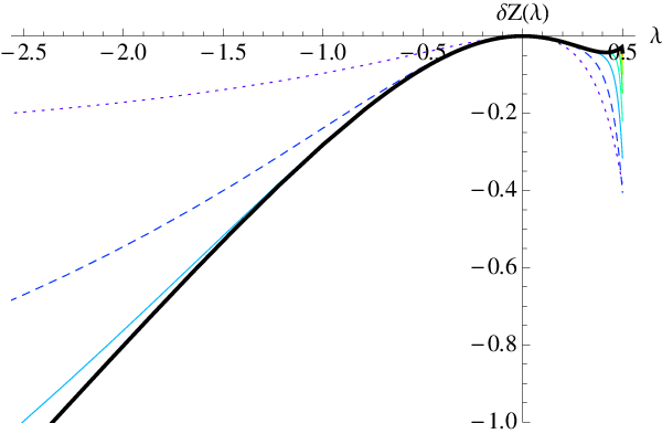
Refer to caption
Figure 10: Plot of δ​Z​(λ)\delta Z(\lambda) defined in equation (351). For real λ\lambda the function δ​Z​(λ)\delta Z(\lambda) is defined for λ∈]−∞,1[\lambda\in]-\infty,1[, with a singularity at λ=1\lambda=1. The Taylor series in κ\kappa has convergence radius 1, which translates into convergence for λ\lambda from −∞-\infty to 1/21/2. This is plotted with an upper bound on the series nmax=2in_{\mathrm{max}}=2^{i}, for i=1,2,…,10i=1,2,...,10, starting with the dotted curve for i=1i=1, dashed for i=2i=2, the remaining ones solid, and finally i=10i=10 (fat). This establishes convergence in that interval. The last 6 curves are indistinguishable, except at λ→1/2\lambda\to 1/2. See figure 13 for the resulting function. Note that δ​Z​(λ)\delta Z(\lambda) can be obtained numerically from the alternative formula (615) with excellent agreement.

The series for δ​Z​(λ)\delta Z(\lambda), defined in Eq. (351), as a series in κ\kappa, has convergence radius 1, since an/an+1→1a_{n}/a_{n+1}\to 1 at large nn, equivalent to ℜ⁡(λ)<12\Re(\lambda)<\frac{1}{2}. This is demonstrated on Fig. 10. The physical singularity however is outside of this interval, at λ=1\lambda=1.

We now obtain the avalanche-size distribution. As explained in section III.3.1, we have

P⁡(u˙)=(1−p′​v)​δ​(u˙)+v​p′​𝒫​(u˙)+O⁡(v2)P(\dot{u})=(1-p^{\prime}v)\delta(\dot{u})+vp^{\prime}{{\cal P}}(\dot{u})+O(v^{2}) (365)

with

Z⁡(λ)=p′​∫0∞d​u˙​(eλ​u˙−1)​𝒫​(u˙).Z(\lambda)=p^{\prime}\int_{0}^{\infty}{\mathrm{d}}\dot{u}(e^{\lambda\dot{u}}-1){{\cal P}}(\dot{u})\ . (366)

We have obtained the expansion of Z⁡(λ)Z(\lambda) to order O⁡(α)O(\alpha) in the form (337), hence

p′​𝒫​(u˙)\displaystyle p^{\prime}{{\cal P}}(\dot{u}) =\displaystyle= 1u˙​e−u˙+α2​δ​𝒫​(u˙),\displaystyle\frac{1}{\dot{u}}e^{-\dot{u}}+\frac{\alpha}{2}\delta{{\cal P}}(\dot{u})\ , (367)
δ​Z​(λ)\displaystyle\delta Z(\lambda) =\displaystyle= ∫0∞d​u˙​(eλ​u˙−1)​δ​𝒫​(u˙).\displaystyle\int_{0}^{\infty}{\mathrm{d}}\dot{u}(e^{\lambda\dot{u}}-1)\,\delta{{\cal P}}(\dot{u})\ . (368)

In the case where δ​Z​(λ)\delta Z(\lambda) admits an inverse Laplace transform we can also write

𝒫⁡(u˙)=𝒫MF​(u˙)+α2​δ​𝒫​(u˙).{\cal P}(\dot{u})={\cal P}_{\rm MF}(\dot{u})+\frac{\alpha}{2}\delta{{\cal P}}(\dot{u})\ . (369)

For u˙>0\dot{u}>0 the inversion reads

δ​𝒫​(u˙)=∫i​∞−i​∞d​λ2​π​i​δ​Z​(λ)​e−λ​u˙,\delta{\cal P}(\dot{u})=\int_{i\infty}^{-i\infty}\frac{{\mathrm{d}}\lambda}{2\pi i}\delta Z(\lambda){\mathrm{e}}^{-\lambda\dot{u}}\ , (370)

the contour being closed to the right. Note that

δ​Z​(λ=0)=0\displaystyle\delta Z(\lambda=0)=0\quad ⇔\displaystyle\Leftrightarrow ∫d​u˙​δ​𝒫​(u˙)=0,\displaystyle\quad\int{\mathrm{d}}\dot{u}\,\delta{{\cal P}}(\dot{u})=0\ , (371)
δ​Z′​(λ=0)=0\displaystyle\delta Z^{\prime}(\lambda=0)=0\quad ⇔\displaystyle\Leftrightarrow ∫d​u˙​u˙​δ​𝒫​(u˙)=0.\displaystyle\quad\int{\mathrm{d}}\dot{u}\,\dot{u}\,\delta{{\cal P}}(\dot{u})=0\ . (372)

To construct the probability distribution we first note the inverse Laplace transform

LT−λ→u˙−1​κn\displaystyle\mbox{LT}^{-1}_{-\lambda\to\dot{u}}\kappa^{n} =\displaystyle= δ⁡(u˙)−n1​F1​(1+n,2,−u˙)\displaystyle\delta(\dot{u})-n~_{1}F_{1}(1+n,2,-\dot{u}) (373)
=\displaystyle= δ⁡(u˙)+e−u˙​∂u˙Ln​(u˙)\displaystyle\delta(\dot{u})+{\mathrm{e}}^{-\dot{u}}\partial_{\dot{u}}\mathrm{L}_{n}(\dot{u})

in terms of the hypergeometric function F11{}_{1}F_{1}, or equivalently the Laguerre-polynomial Ln\mathrm{L}_{n}. For u˙>0\dot{u}>0 it can be found by rewriting the contour integral (which with our conventions must be closed to the right):

∫i​∞−i​∞d​λ2​π​i​(−λ1−λ)n​e−λ​u˙\displaystyle\int_{i\infty}^{-i\infty}\frac{{\mathrm{d}}\lambda}{2\pi i}\left(\frac{-\lambda}{1-\lambda}\right)^{n}{\mathrm{e}}^{-\lambda\dot{u}}
=\displaystyle= (∂∂v)n​∫0∞d​α​∫i​∞−i​∞d​λ2​π​i​e−λ​u˙−α⁡(1−λ)​αn−1Γ⁡(α)\displaystyle\left(\frac{\partial}{\partial{v}}\right)^{n}\int_{0}^{\infty}{\mathrm{d}}\alpha\int_{i\infty}^{-i\infty}\frac{{\mathrm{d}}\lambda}{2\pi i}{\mathrm{e}}^{-\lambda\dot{u}-\alpha(1-\lambda)}\frac{\alpha^{n-1}}{\Gamma(\alpha)}
=\displaystyle= (∂∂u˙)n​u˙n−1​e−u˙Γ⁡(n)\displaystyle\left(\frac{\partial}{\partial{\dot{u}}}\right)^{n}\frac{\dot{u}^{n-1}{\mathrm{e}}^{-\dot{u}}}{\Gamma(n)}

leading to (373). Thus we can now write the formal series

δ​𝒫​(u˙)=∑n=2∞an​e−u˙​∂u˙Ln​(u˙).\delta{{\cal P}}(\dot{u})=\sum_{n=2}^{\infty}a_{n}{\mathrm{e}}^{-\dot{u}}\partial_{\dot{u}}\mathrm{L}_{n}(\dot{u})\ . (374)

Unfortunately, this series is divergent.

This problem can be cured as follows: We will subtract from the series (351) terms which can be summed analytically, resulting in polylogarithmic functions, and their derivatives, and inverting the latter via a cut-integral. These terms are chosen to render the remaining sum (quasi-)convergent. To this aim, we note

δ​Z​(λ)=δ​Zser​(λ)+δ​Zcut​(λ).\delta Z(\lambda)=\delta Z_{\mathrm{ser}}(\lambda)+\delta Z_{\mathrm{cut}}(\lambda)\ . (375)

We start by Taylor-expanding ana_{n} around n=∞n=\infty,

an\displaystyle a_{n} =\displaystyle= 1−4​ln⁡(2​n)2​n+2n2+6​ln⁡(2)−3712n3+5−6​ln⁡(2)n4\displaystyle\frac{{1}-4\ln(2n)}{2n}+\frac{2}{n^{2}}+\frac{6\ln(2)-\frac{37}{12}}{n^{3}}+\frac{5-6\ln(2)}{n^{4}} (376)
+6​ln⁡(2)−10130n5+O⁡(1n6)\displaystyle+\frac{6\ln(2)-\frac{101}{30}}{n^{5}}+O\Big(\frac{1}{n^{6}}\Big)
=−2​ln⁡nn+∑j=1∞bjnj\displaystyle=-\frac{2\ln n}{n}+\sum_{j=1}^{\infty}\frac{b_{j}}{n^{j}}

with b1=12−2​ln⁡2b_{1}=\frac{1}{2}-2\ln 2, b2=2b_{2}=2, and an explicit formula for bjb_{j} for j≥3j\geq 3 is given in Appendix N. We recall that a2=1−2​ln⁡2a_{2}=1-2\ln 2 and that we set a1=0a_{1}=0 2626 26 Although this may appear to impose an artificial constraint ∑j=1∞bj=0\sum_{j=1}^{\infty}b_{j}=0 it will be immaterial in what follows since we will use only a finite sum and add and subtract the same terms..

Refer to caption
Figure 11: u˙​δ​P​(u˙)\dot{u}\delta P(\dot{u}) as given by Eq. (380), or, equivalently by Eq. (616).

Performing the summation, we obtain (if the series converges) the alternative representation

δ​Z​(λ)=2​∂jLij​(κ)|j=1+∑j=1∞bj​Lij​(κ).\delta Z(\lambda)=2\partial_{j}{\rm Li}_{j}(\kappa)\big|_{j=1}+\sum_{j=1}^{\infty}b_{j}{\rm Li}_{j}(\kappa)\ . (377)

Lij​(κ){\rm Li}_{j}(\kappa) is the polylogarithm function, which is analytic on the complex plane with a cut on the real axis for κ∈[1,∞[\kappa\in[1,\infty[, which maps on the same interval for λ∈[1,∞[\lambda\in[1,\infty[ with reversed boundaries. It is along this cut that we have to integrate. The discontinuity there is given by

limϵ→0+Lij​(κ+i​ϵ)−Lij​(κ−i​ϵ)={2​π​i​(ln⁡κ)j−1Γ⁡(j),κ>1,0,κ<1..\lim_{\epsilon\to 0^{+}}{\rm Li}_{j}(\kappa+i\epsilon)-{\rm Li}_{j}(\kappa-i\epsilon)=\begin{cases}2\pi i\frac{(\ln\kappa)^{j-1}}{\Gamma(j)}\,,&\kappa>1\,,\\ 0\,,&\kappa<1\,.\end{cases}\ . (378)

Note that this also holds true for the derivative w.r.t. jj, and for j=1j=1, i.e. Li1​(κ)=−ln⁡(1−κ)\mbox{Li}_{1}(\kappa)=-\ln(1-\kappa).

Thus, the inverse Laplace transform (370) becomes a compact and simple cut-integral

δ​𝒫​(u˙)\displaystyle\delta{\cal P}(\dot{u}) =−∫1∞d​λeλ​v[2γE+2ln(lnκ)+∑j=1∞bj​(ln⁡κ)j−1Γ⁡(j)]\displaystyle=-\int\limits_{1}^{\infty}\frac{{\mathrm{d}}\lambda}{{\mathrm{e}}^{\lambda v}}\left[2\gamma_{\mathrm{E}}+2\ln(\ln\kappa)+\sum_{j=1}^{\infty}\frac{b_{j}(\ln\kappa)^{j-1}}{\Gamma(j)}\right] (379)

However, this series also diverges. Therefore we choose jmaxj_{\mathrm{max}} as a cutoff, by defining

δ​𝒫​(u˙)\displaystyle\delta{\cal P}(\dot{u}) =\displaystyle= δ​𝒫ser​(u˙)+δ​𝒫cut​(u˙)\displaystyle\delta{\cal P}_{\mathrm{ser}}(\dot{u})+\delta{\cal P}_{\mathrm{cut}}(\dot{u}) (380)
δ​𝒫cut​(u˙)\displaystyle\delta{\cal P}_{\mathrm{cut}}(\dot{u}) =\displaystyle= −∫1∞d​λeλ​v[2γE+2ln(lnκ)+∑j=1jmaxbj​(ln⁡κ)j−1Γ⁡(j)]\displaystyle-\int\limits_{1}^{\infty}\frac{{\mathrm{d}}\lambda}{{\mathrm{e}}^{\lambda v}}\left[2\gamma_{\mathrm{E}}+2\ln(\ln\kappa)+\sum_{j=1}^{j_{\mathrm{max}}}\frac{b_{j}(\ln\kappa)^{j-1}}{\Gamma(j)}\right]
Refer to caption
Refer to caption
Figure 12: Left: 𝒫⁡(u˙)​u˙a{\cal P}(\dot{u})\dot{u}^{\rm a} as a function of u˙a\dot{u}^{\rm a} for RF-disorder; ϵ=0\epsilon=0 i.e. MF (black dashed), ϵ=1\epsilon=1 (blue, dotted), ϵ=2\epsilon=2 (green, dash-dotted) and ϵ=3\epsilon=3 (red, solid). Right: log-log plot of 𝒫⁡(u˙){\cal P}(\dot{u}) as a function of u˙\dot{u}, for the same values of ϵ\epsilon. For both plots resummation formula (385) was used. We note that since only α\alpha appears as a parameter, at this order ϵ=3\epsilon=3 RF and ϵ=2\epsilon=2 RP are indistinguishable, see Eqs. (360), (361).

The coefficients a~n\tilde{a}_{n} are what remains of ana_{n} after subtracting their asymptotic behavior,

a~n:=an+2​ln⁡nn−∑j=1jmaxbjnj.\tilde{a}_{n}:=a_{n}+2\frac{\ln n}{n}-\sum_{j=1}^{j_{\mathrm{max}}}\frac{b_{j}}{n^{j}}\ . (382)

Especially note that a~1\tilde{a}_{1} becomes non-zero, even though a1=0a_{1}=0; in fact, this coefficient grows rather quickly with jmaxj_{\mathrm{max}}, while the other coefficients decay.

δ​𝒫ser​(u˙)=∑n=1∞a~n​e−u˙​∂u˙Ln​(u˙).\delta{\cal P}_{\mathrm{ser}}(\dot{u})=\sum_{n=1}^{\infty}\tilde{a}_{n}{\mathrm{e}}^{-\dot{u}}\partial_{\dot{u}}\mathrm{L}_{n}(\dot{u})\ . (383)

Both expressions, δ​𝒫cut​(u˙)\delta{\cal P}_{\mathrm{cut}}(\dot{u}) and δ​𝒫ser​(u˙)\delta{\cal P}_{\mathrm{ser}}(\dot{u}) can be obtained numerically with good precision, and seem to decay rapidly at large u˙\dot{u}. One then checks that the sum of the two, for any u˙\dot{u} in the bulk of the distribution, converges extremely well versus the result at j=jmaxj=j_{\mathrm{max}}, e.g. for u˙=1\dot{u}=1 excellent precision is already obtained for jmax=3j_{\rm max=3}. Of course, for a fixed jmaxj_{\mathrm{max}} the sum over nn in (383) should be stopped at nn not too large since it is an asymptotic series, which is ultimately divergent, but in practice the range of convergence (with respect to nmaxn_{\rm max}) is rather broad.

Practical values are jmax=15j_{\mathrm{max}}=15, and (383) can also be stopped at n=15n=15. With this choice, we find that the precision is excellent and that all moments ∫0∞u˙p​δ​P​(u˙)​𝑑u˙\int_{0}^{\infty}\dot{u}^{p}\delta P(\dot{u}){\mathrm{d}}\dot{u} between the fourth and 36th are at least given with a relative precision of 10−710^{-7}, most even of 10−1010^{-10}. jmaxj_{\mathrm{max}} should not be taken too large, since otherwise this shifts too much weight into the moment a~1\tilde{a}_{1}, leading to numerical problems (cancelation of large terms.) As an example, for jmax=15j_{\max}=15, one has a~1=−51.97\tilde{a}_{1}=-51.97, a~2=0.002976\tilde{a}_{2}=0.002976, a~3=1.359×10⁻⁶\tilde{a}_{3}=1.359\times 10^{-6}, …, a~20=2.373×10⁻¹⁵\tilde{a}_{20}=2.373\times 10^{-15}. There are no convergence problems at small or large u˙\dot{u}.

The final result for 𝒫⁡(u˙){\cal P}(\dot{u}) is

𝒫⁡(u˙)\displaystyle{\cal P}(\dot{u}) =\displaystyle= 𝒫0​(u˙)+α2​δ​𝒫​(u˙)+O⁡(ϵ2)\displaystyle{\cal P}_{0}(\dot{u})+\frac{\alpha}{2}\delta{\cal P}(\dot{u})+O(\epsilon^{2}) (384)
=\displaystyle= 𝒫0​(u˙)​exp⁡(α2​δ​𝒫​(u˙)𝒫0​(u˙))+O⁡(ϵ2),\displaystyle{\cal P}_{0}(\dot{u})\exp\left(\frac{\alpha}{2}\frac{\delta{\cal P}(\dot{u})}{{\cal P}_{0}(\dot{u})}\right)+O(\epsilon^{2})\ ,\qquad (385)

where we remind the value of the small parameter α\alpha from (358). Note that the second formula (385), while being equivalent to order ϵ\epsilon, has the property to resum the logarithmic behavior at small vv into the correct power-law behavior. This is why we have chosen it in Fig. 12.

Refer to caption
Figure 13: (Color online) δ​Z​(λ)\delta Z(\lambda), as obtained by (351) (thick red line), a reexpansion in λ\lambda (dashed thick green line) and numerical integration of Eq. (368), using Eq. (380) (thin black line). All functions agree in their respective area of convergence.

IV.4.3 Small-velocity behaviour, the critical exponent 𝖺{\sf a}

Let us now obtain the small-velocity asymptotics of P⁡(u˙)P(\dot{u}) and extract the a-priori new critical exponent 𝖺{\sf a}. It is controlled by the asymptotics of δ​Z​(λ)\delta Z(\lambda) at large negative λ\lambda, i.e. λ→−∞\lambda\to-\infty. This corresponds to the behaviour for κ→1−\kappa\to 1^{-} of the series (351). It is determined by the leading behaviour of ana_{n} at large nn, i.e. from the leading term an=−2ln(n)/na_{n}=-2\ln(n)/n of (376). Resumming with this term alone, we obtain

δ​Z​(λ)\displaystyle\delta Z(\lambda) =\displaystyle= ∑n=2∞anκn≈−2∑n=2∞ln⁡(n)nκn=2∂aLia(κ)|a=1\displaystyle\sum_{n=2}^{\infty}a_{n}\kappa^{n}\approx-2\sum_{n=2}^{\infty}\frac{\ln(n)}{n}\kappa^{n}=2\partial_{a}\mbox{Li}_{a}(\kappa)\big|_{a=1} (386)
=\displaystyle= −ln2⁡(1−κ)+O⁡(ln⁡(1−κ))+…\displaystyle-\ln^{2}(1-\kappa)+O\Big(\ln(1-\kappa)\Big)+\dots
=\displaystyle= −ln2⁡(1−λ)+….\displaystyle-\ln^{2}(1-\lambda)+\dots\ .

This yields for λ→−∞\lambda\to-\infty

Z⁡(λ)\displaystyle Z(\lambda) =\displaystyle= Z0​(λ)+α2​δ​Z​(λ)\displaystyle Z_{0}(\lambda)+\frac{\alpha}{2}\delta Z(\lambda) (387)
=\displaystyle= −ln⁡(1−λ)​[1+α2​ln⁡(1−λ)+…].\displaystyle-\ln(1-\lambda)\left[1+\frac{\alpha}{2}\ln(1-\lambda)+\dots\right]\ .~~~~~~

It is easy to see that this is consistent with a modified critical behaviour at small velocities

𝒫(u˙)∼u˙≪11u˙𝖺,𝖺=1+α+O(ϵ2).{\cal P}(\dot{u})\sim_{\dot{u}\ll 1}\frac{1}{\dot{u}^{\sf a}}\quad,\quad{\sf a}=1+\alpha+O(\epsilon^{2})\ . (388)

To show this, we start from the trial probability

p′​𝒫trial​(u˙)=1u˙1+x​e−u˙p^{\prime}{{\cal P}}_{\rm trial}(\dot{u})=\frac{1}{\dot{u}^{1+x}}e^{-\dot{u}} (389)

for which the associated Z⁡(λ)Z(\lambda) can be computed exactly via a Laplace transform, using (366). Expanding the result in small xx yields

Ztrial​(λ)\displaystyle Z_{\rm trial}(\lambda) =\displaystyle= ∫0∞d​u˙​1u˙1+x​e−u˙​(eλ​u˙−1)\displaystyle\int_{0}^{\infty}{\mathrm{d}}\dot{u}\frac{1}{\dot{u}^{1+x}}e^{-\dot{u}}(e^{\lambda\dot{u}}-1) (390)
=\displaystyle= −ln⁡(1−λ)\displaystyle-\ln(1-\lambda)
+[−γE+ln⁡(1−λ)−12​ln2⁡(1−λ)]​x\displaystyle+\left[-\gamma_{\rm E}+\ln(1-\lambda)-\frac{1}{2}\ln^{2}(1-\lambda)\right]x
+O⁡(x2)\displaystyle+O(x^{2})

the first term is Ztree​(λ)Z^{\mathrm{tree}}(\lambda) and the second one the correction. Comparing the behavior at large negative λ\lambda of Eqs. (387) and (390), we can thus identify x=αx=\alpha, consistent with Eq. (388). Note that multiplying (389) by a prefactor Cx=1+O⁡(x)C_{x}=1+O(x) or changing the exponential to e−u˙​[1+O​(x)]e^{-\dot{u}[1+O(x)]} produces only ∼x​ln⁡(λ)\sim x\ln(\lambda) terms, subdominant w.r.t. the ln2⁡(1−λ)\ln^{2}(1-\lambda) at λ→−∞\lambda\to-\infty.

Let us now discuss our results for the small-velocity exponent. Using (388), together with (360) and (361), we find

𝖺=1−29​ϵ+O⁡(ϵ2)nonperiodic\displaystyle{\sf a}=1-\frac{2}{9}\epsilon+O(\epsilon^{2})\quad{\rm nonperiodic} (391)
𝖺=1−13​ϵ+O⁡(ϵ2)periodic.\displaystyle{\sf a}=1-\frac{1}{3}\epsilon+O(\epsilon^{2})\quad{\rm periodic}\ . (392)

Our predictions for the change of 𝖺{\sf a} are thus quite large, and tend to reduce the exponent. A naive extrapolation to d=1d=1, ϵ=3\epsilon=3 (depinning of a line) would suggest 𝖺≈1/3{\sf a}\approx 1/3 significantly reduced from the mean-field value 𝖺MF=1{\sf a}_{\rm MF}=1. Preliminary numerical results indicate that the exponent 𝖺{\sf a} may even be negative in d=1d=1 [100]. A 2-loop calculation (or higher) would settle the question from an analytical point of view.

We can compare the above formula to the one for the dynamical exponent to one loop

z=2+α+O⁡(ϵ2).z=2+\alpha+O(\epsilon^{2})\ . (393)

Hence we could also write

𝖺=z−1+O⁡(ϵ2),{\sf a}=z-1+O(\epsilon^{2})\ , (394)

which holds for both periodic and non-periodic systems. Again it would be interesting to obtain the higher-loop corrections, since we did not find any general argument why they would be absent.

Finally the small-u˙\dot{u} behaviour can be studied more systematically. This is done in Appendix O where we obtain the amplitude at small u˙>0\dot{u}>0,

P⁡(u˙)≈Cu˙𝖺,C=1−α2​(4​γE+b1)P(\dot{u})\approx\frac{C}{\dot{u}^{{\sf a}}}\quad,\quad C=1-\frac{\alpha}{2}(4\gamma_{\rm E}+b_{1}) (395)

where b1=12−2​ln⁡2b_{1}=\frac{1}{2}-2\ln 2 as defined above. This yields C=1−0.711284​αC=1-0.711284\alpha in good agreement with our numerical Laplace-inversion. In principle this amplitude is universal and can be measured.

IV.4.4 The behavior of δ​Z​(λ)\delta Z(\lambda) for λ→1\lambda\to 1, and tail of 𝒫⁡(u˙){\cal P}(\dot{u}) at large u˙\dot{u}

The behavior of Z⁡(λ)Z(\lambda) in the limit of λ→1\lambda\to 1, which controls the tail of 𝒫⁡(u˙){\cal P}(\dot{u}) for u˙→∞\dot{u}\to\infty, is obtained in Appendix G. The final result is

Z⁡(λ)\displaystyle Z(\lambda) =\displaystyle= −ln⁡(1−λ)+α2​δ​Z​(λ)\displaystyle-\ln(1-\lambda)+\frac{\alpha}{2}\delta Z(\lambda) (396)
δ​Z​(λ)\displaystyle\delta Z(\lambda) =\displaystyle= 18​1(1−λ)2​[ln⁡(1−λ)]2+…\displaystyle\frac{1}{8}\frac{1}{(1-\lambda)^{2}[\ln(1-\lambda)]^{2}}+... (397)

To obtain the tail of 𝒫⁡(u˙){\cal P}(\dot{u}), one needs to inverse Laplace tranform Z⁡(λ)Z(\lambda). Before doing so, let us point out that this form is incompatible with the naive expectation of a stretched exponential at large velocity,

P(u˙)∼u˙≫1C′u˙𝖺′e−B​u˙δ,P(\dot{u})\sim_{\dot{u}\gg 1}\frac{C^{\prime}}{\dot{u}^{{\sf a}^{\prime}}}e^{-B\dot{u}^{\delta}}\ , (398)

with C′=B=𝖺′=δ=1C^{\prime}=B={\sf a}^{\prime}=\delta=1 in mean field (ϵ=0\epsilon=0). While it would be hard to extract B,C′B,C^{\prime} and 𝖺′{\sf a}^{\prime}, we could extract δ\delta as follows. Expanding near δ=1,\delta=1, we find

α2​δ​𝒫​(u˙)=−(δ−1)​e−u˙​ln⁡u˙+O⁡((δ−1)2).\frac{\alpha}{2}\delta{\cal P}(\dot{u})=-(\delta-1){\mathrm{e}}^{-\dot{u}}\ln\dot{u}+O((\delta-1)^{2})\ . (399)

This is equivalent to

α2​δ​Z​(λ)=(δ−1)​ln⁡(1−λ)+γE​λ1−λ+O⁡((δ−1)2).\frac{\alpha}{2}\delta Z(\lambda)=(\delta-1)\frac{\ln(1-\lambda)+\gamma_{\rm E}\lambda}{1-\lambda}+O((\delta-1)^{2})\ . (400)

Clearly, this is not of the form (397). Noting s:=1−λs:=1-\lambda, we claim that Eq. (397) is equivalent to

δ​𝒫​(u˙)≃18​e−u˙​u˙2​f​(u˙)\delta{\cal P}(\dot{u})\simeq\frac{1}{8}e^{-\dot{u}}\dot{u}^{2}f(\dot{u}) (401)

at large u˙\dot{u}, where f⁡(u˙)f(\dot{u}) has a Laplace transform f^​(s):=∫0∞d​u˙​f​(u˙)​e−s​u˙\hat{f}(s):=\int_{0}^{\infty}{\mathrm{d}}{\dot{u}}f({\dot{u}}){\mathrm{e}}^{-s{\dot{u}}} which behaves at small ss as

f^​(s)=f^​(0)+1ln⁡s.\hat{f}(s)=\hat{f}(0)+\frac{1}{\ln s}\ . (402)

Indeed that would imply

LTu˙→s​eu˙​δ​𝒫​(u˙)=18​∂s2f^​(s)≃18​1s2​(ln⁡s)2{\rm LT}_{\dot{u}\to s}e^{\dot{u}}\delta{\cal P}(\dot{u})=\frac{1}{8}\partial_{s}^{2}\hat{f}(s)\simeq\frac{1}{8}\frac{1}{s^{2}(\ln s)^{2}} (403)

for small ss, which is exactly the result (397). It is then easy to guess that

f⁡(u˙)=1u˙​(ln⁡u˙)2=−∂∂u˙​1ln⁡u˙f(\dot{u})=\frac{1}{\dot{u}(\ln\dot{u})^{2}}=-\frac{\partial}{\partial{\dot{u}}}\frac{1}{\ln{\dot{u}}} (404)

at large u˙\dot{u}, for u˙>u˙0\dot{u}>\dot{u}_{0}. Indeed, the contribution for u˙>u˙0\dot{u}>\dot{u}_{0} reads

f^​(0)−f^​(s)\displaystyle\hat{f}(0)-\hat{f}(s) =\displaystyle= −∫u˙0∞du˙(1−e−s​u˙)∂∂u˙1ln⁡u˙\displaystyle-\int_{{\dot{u}}_{0}}^{\infty}{\mathrm{d}}{\dot{u}}\,(1-e^{-s\dot{u}})\frac{\partial}{\partial{\dot{u}}}\frac{1}{\ln{\dot{u}}} (405)
≃\displaystyle\simeq ∫u˙0∞d​u˙​s​e−s​u˙​1ln⁡u˙\displaystyle\int_{\dot{u}_{0}}^{\infty}{\mathrm{d}}{\dot{u}}\,s\,e^{-s\dot{u}}\frac{1}{\ln{\dot{u}}}
=\displaystyle= ∫u˙0​s∞d​w​e−w​1ln⁡w−ln⁡s\displaystyle\int_{\dot{u}_{0}s}^{\infty}{\mathrm{d}}w\,e^{-w}\frac{1}{\ln w-\ln s}
≃\displaystyle\simeq −1ln⁡s.\displaystyle-\frac{1}{\ln s}\ .

In the partial integration from the first to the second line we have dropped a term (1−e−s​u˙0)/ln⁡u˙0(1-e^{-s\dot{u}_{0}})/\ln{\dot{u}}_{0}, which is of order ss. In the last step, we have used that for s→0s\to 0, first ln⁡w−ln⁡s≈−ln⁡s\ln w-\ln s\approx-\ln s, and second u˙0​s→0\dot{u}_{0}s\to 0.

For the velocity distribution at large u˙\dot{u}, we thus finally obtain

𝒫u˙→∞1−loop​(u˙)\displaystyle{\cal P}^{\rm{1-loop}}_{\dot{u}\to\infty}(\dot{u}) =\displaystyle= e−u˙u˙​[1+α16​u˙2ln2⁡(u˙)]+O⁡(α2)\displaystyle\frac{{\mathrm{e}}^{-\dot{u}}}{\dot{u}}\left[1+\frac{\alpha}{16}\frac{\dot{u}^{2}}{\ln^{2}(\dot{u})}\right]+O(\alpha^{2}) (406)
=\displaystyle= e−u˙u˙​exp⁡(α16​u˙2ln2⁡(u˙))+O⁡(α2)\displaystyle\frac{{\mathrm{e}}^{-\dot{u}}}{\dot{u}}\exp\left(\frac{\alpha}{16}\frac{\dot{u}^{2}}{\ln^{2}(\dot{u})}\right)+O(\alpha^{2})~~~~~~~~~

We remind that α<0\alpha<0, which has motivated us to write the result in an exponentiated form. Other forms are however possible, such as corrections to the pre-exponential only. The form (406) renders the tail stronger decaying; it is plotted on figure 14. In all cases, given the smallness of the correction, this tail will be hard to see in numerical simulations. With the help of Eq. (380), we have been able to evaluate δ​𝒫​(u˙)\delta{\cal P}({\dot{u}}) up to u˙≈100{\dot{u}}\approx 100, while the alternative representation (616) works up to u˙≈10{\dot{u}}\approx 10. For these values of u˙{\dot{u}}, the tail-behavior (406) is not yet reached.

Refer to caption
Figure 14: The exponentiated version (406) of the function 𝒫u˙→∞1−loop​(u˙){\cal P}^{\mathrm{1-loop}}_{\dot{u}\to\infty}(\dot{u}) for α=−23\alpha=-\frac{2}{3} (e.g. RF disorder in d=1d=1) (red dashed line), compared to the mean-field result (i.e. ϵ=0\epsilon=0, blue, solid line).

IV.4.5 Alternative approach: Integrating over momentum first

Our result for δ​Z​(λ)\delta Z(\lambda) given in Eq. (351), was a compact series expansion from which one first had to extract the asymptotic behavior at large λ\lambda, before being able to perform the inverse Laplace transform. A complementary approach, performed in detail in appendix H, is to start from Eq. (330), calculate Φ⁡(k,t)\Phi(k,t) as given in Eq. (340), and first integrate over tt and kk, the final result for δ​Z​(λ)\delta Z(\lambda), given in (615), is now an integral over t1t_{1}. (Recall that above in Eqs. (341) and (342) we integrated first over tt, and t1t_{1} leaving the kk integral for the end). We did not succeed in performing the final integral over t1t_{1} analytically, although it is easy to compute numerically. It confirms the above results for δ​Z​(λ)\delta Z(\lambda). The advantage of this method is that the inverse-Laplace transform can be done explicitly, yielding a (relatively complicated) integral representation (as integral over t1t_{1}) of δ​𝒫​(u˙)\delta{\cal P}({\dot{u}}) given in (616). It confirms all statements made above, including the asymptotic behavior for small and large u˙\dot{u}.

Note that in Eqs. (341) and (342) one can interpret tt as the time of a kick (infinitesimal step in the force), or starting time of the avalanche, while time zero is the measurement time. The time t1<0t_{1}<0 is an intermediate time, which must be integrated over the duration of the avalanche. Hence, if we instead integrate over kk and then t1∈[t,0]t_{1}\in[t,0] at fixed tt we obtain the joint probability that u˙​(0)=u˙\dot{u}(0)=\dot{u} and the avalanche started at tt. Although it is a straightforward generalization we will not give this result here.

IV.5 Recovering the avalanche-size distribution to one-loop

As discussed in section III.6, to recover the avalanche-size distribution, one can use a source constant in time λx​t=λ\lambda_{xt}=\lambda during a large time window TT. The avalanche-size generating function, noted here ZS​(λ),Z_{S}(\lambda), is obtained from the dynamic generating function studied here via Z⁡[λ]=T​ZS​(λ)Z[\lambda]=TZ_{S}(\lambda). In practice it amounts to suppressing the final time integral in the expression for Z⁡[λ]Z[\lambda].

For a source constant in time, the solution of the unperturbed instanton equation (ηx=0\eta_{x}=0) is

u~0=ZS0≡ZS0​(λ)=12​(1−1−4​λ).\tilde{u}^{0}=Z_{S}^{0}\equiv Z_{S}^{0}(\lambda)=\frac{1}{2}(1-\sqrt{1-4\lambda})\ . (407)

The dressed response kernel then becomes

ℝk,t2,t1=e−(k2+1−2​ZS0)​(t2−t1)​θ​(t2−t1),\mathbb{R}_{k,t_{2},t_{1}}=e^{-(k^{2}+1-2Z_{S}^{0})(t_{2}-t_{1})}\theta(t_{2}-t_{1})\ , (408)

which is simply the bare response up to the replacement m2→m2−2​ZS0​(λ)m^{2}\to m^{2}-2Z_{S}^{0}(\lambda). The formula (328) then gives

Φ⁡(k,t1)=ZS0​∫t1<t2ℝk,t2,t1=ZS0k2+1−2​ZS0.\Phi(k,t_{1})=Z_{S}^{0}\int_{t_{1}<t_{2}}{\mathbb{R}}_{k,t_{2},t_{1}}=\frac{Z^{0}_{S}}{k^{2}+1-2Z^{0}_{S}}\ . (409)

Following the steps in Section IV.3.2, this leads to

ZS\displaystyle Z_{S} =\displaystyle= ZS0+ZS1+…\displaystyle Z_{S}^{0}+Z_{S}^{1}+... (410)
ZS1\displaystyle Z^{1}_{S} =\displaystyle= ⟨u~x​t(2)⟩η=αϵ​I~2​∫k𝒥t​(k)\displaystyle\langle\tilde{u}^{(2)}_{xt}\rangle_{\eta}=\frac{\alpha}{\epsilon\tilde{I}_{2}}\int_{k}{\cal J}_{t}(k) (411)
𝒥t​(k)\displaystyle{\cal J}_{t}(k) =\displaystyle= 11−2​ZS0​𝒥ta​(k).\displaystyle\frac{1}{1-2Z^{0}_{S}}{\cal J}^{a}_{t}(k)\ . (412)

The coefficient A=αϵ​I~2A=\frac{\alpha}{\epsilon\tilde{I}_{2}}, and we have defined

𝒥ta​(k)=(ZS0k2+1−2​ZS0)2+ZS0k2+1−2​ZS0,{\cal J}^{a}_{t}(k)=\bigg(\frac{Z^{0}_{S}}{k^{2}+1-2Z^{0}_{S}}\bigg)^{\!2}+\frac{Z^{0}_{S}}{k^{2}+1-2Z^{0}_{S}}\ , (413)

which is time independent. Graphically Eq. (412) can be written as in (IV.3.1),

ZS1=αϵ​I~2​[(ZS0)2​[Uncaptioned image]+ZS0​[Uncaptioned image]],Z_{S}^{1}=\frac{\alpha}{\epsilon\tilde{I}_{2}}\left[(Z^{0}_{S})^{2}\parbox{37.24228pt}{\hskip 3.44444pt\includegraphics[scale={0.35}]{./figures/stat1+}\hskip 3.44444pt}+Z^{0}_{S}\parbox{26.40178pt}{\hskip 3.44444pt\includegraphics[scale={0.35}]{./figures/stat2+}\hskip 3.44444pt}\right]\ , (414)

replacing the external wiggly lines of Eq. (IV.3.1) by the factors ZS0Z^{0}_{S}. Note that we have recovered Eq. (152) of [74] for the statics, up to the two counter-terms discussed below. For pedagogical purposes, we want to make further contact with the self-consistent equation obtained in [73]. To this aim we rewrite Eq. (412) as

αϵ​I~2​∫k𝒥ta​(k)\displaystyle\frac{\alpha}{\epsilon\tilde{I}_{2}}\int_{k}{\cal J}_{t}^{a}(k) =\displaystyle= ZS1​(1−2​ZS0)\displaystyle Z^{1}_{S}(1-2Z_{S}^{0}) (415)
=\displaystyle= (ZS−ZS0+…)​(1−ZS0−ZS+…)\displaystyle(Z_{S}-Z_{S}^{0}+...)(1-Z_{S}^{0}-Z_{S}+...)
=\displaystyle= ZS−(ZS)2−[ZS0−(ZS0)2]\displaystyle Z_{S}-(Z_{S})^{2}\ -\left[Z_{S}^{0}-(Z_{S}^{0})^{2}\right]
=\displaystyle= ZS−(ZS)2−λ.\displaystyle Z_{S}-(Z_{S})^{2}\ -\lambda\ .

Note that by going from the first to the second line, we have added in each parenthesis a subdominant term. From the second to the third line, we have regrouped the terms, and finally from the third to the fourth line we used the exact relation ZS0−(ZS0)2=λZ_{S}^{0}-(Z_{S}^{0})^{2}=\lambda. Eq. (415) can thus be written as

ZS\displaystyle Z_{S} =\displaystyle= λ+(ZS)2+αϵ​I~2​∫k𝒥ta​(k).\displaystyle\lambda+(Z_{S})^{2}+\frac{\alpha}{\epsilon\tilde{I}_{2}}\int_{k}{\cal J}_{t}^{a}(k)\ . (416)
=\displaystyle= λ+(ZS)2+αϵ​I~2​[(ZS0)2​[Uncaptioned image]+ZS0​[Uncaptioned image]]\displaystyle\lambda+(Z_{S})^{2}+\frac{\alpha}{\epsilon\tilde{I}_{2}}\left[(Z^{0}_{S})^{2}\parbox{37.24228pt}{\hskip 3.44444pt\includegraphics[scale={0.35}]{./figures/stat1}\hskip 3.44444pt}+Z^{0}_{S}\parbox{24.95639pt}{\hskip 3.44444pt\includegraphics[scale={0.35}]{./figures/stat2}\hskip 3.44444pt}\right]

where we recall the graphical interpretation of each term. (The amputated lower response gave the factor of 1/(1−2​ZS0)1/(1-2Z^{0}_{S}).) Comparison with formula (151) in [73] shows that one recovers the result of the static calculation, provided (i) one replaces in 𝒥ta​(k)\mathcal{J}^{a}_{t}(k) the tree generating function ZS0Z_{S}^{0} by ZSZ_{S}, which does not make a difference at this order; (ii) one adds to Eq. (416) two counter-terms, discussed below,

ZS=λ+(ZS)2+αϵ​I~2​∫k[𝒥ta​(k)+𝒥cta​(k)]\displaystyle Z_{S}=\lambda+(Z_{S})^{2}+\frac{\alpha}{\epsilon\tilde{I}_{2}}\int_{k}\Big[{\cal J}^{a}_{t}(k)+{\cal J}^{a}_{\rm ct}(k)\Big]~~~~~~~~~ (417)
𝒥cta​(k)=−3​(ZS0)2(k2+1)2−ZS0k2+1.\displaystyle{\cal J}^{a}_{\rm ct}(k)=\frac{-3(Z^{0}_{S})^{2}}{(k^{2}+1)^{2}}-\frac{Z^{0}_{S}}{k^{2}+1}\ . (418)

In the statics these counter-terms appeared naturally by using everywhere the improved action. The first one comes from the renormalization of Δ⁡(u)\Delta(u), thus all parameters which appear are renormalized ones. The second also appeared naturally in the statics from the definitions used there, while here it comes as a correction from using the (over)simplified model, as is explained below.

IV.6 Counter-terms and corrections to the simplified theory

IV.6.1 Counter-terms from renormalization

In [73] the static avalanche-size distribution was computed using the improved action, i.e. in terms of the renormalized disorder Δ⁡(u)\Delta(u), which automatically includes the counter-terms for the renormalization of the disorder. In the dynamics, there is an additional operator which is marginal at d=ducd=d_{\rm uc} and corresponds to the friction term in the dynamical action. Computing from the start in terms of the renormalized friction η\eta is possible, but less convenient, hence here we perform the calculation first in terms of the bare disorder Δ0​(u)\Delta_{0}(u) and the bare friction η0\eta_{0}, and then reexpress at the end the result in terms of the renormalized disorder and friction. This yields an explicit derivation of the counter-terms.

We start from the bare action given in Eqs. (81) ff.

𝒮\displaystyle{\cal S} =\displaystyle= ∫x​tu~x​t(η0∂t−∇x2+m2)u˙x​t\displaystyle\int_{xt}\tilde{u}_{xt}(\eta_{0}\partial_{t}-\nabla_{x}^{2}+m^{2})\dot{u}_{xt}
+Δ0′(0+)∫x​tu~x​tu~x​t(v+u˙x​t)\displaystyle+\Delta_{0}^{\prime}(0^{+})\int_{xt}\tilde{u}_{xt}\tilde{u}_{xt}(v+\dot{u}_{xt})
+12Δ0′′(0+)∫x​t​t′u~x​tu~x​t′(v+u˙x​t)(v+u˙x​t′).\displaystyle+\frac{1}{2}\Delta_{0}^{\prime\prime}(0^{+})\int_{xtt^{\prime}}\tilde{u}_{xt}\tilde{u}_{xt^{\prime}}(v+\dot{u}_{xt})(v+\dot{u}_{xt^{\prime}})\ .

Here the subscript zero denotes bare quantities.

The effective action to one loop, Γ=𝒮+δ​𝒮\Gamma={\cal S}+\delta{\cal S}, reads

δ​𝒮=Δ0′′​(0+)​∫x​t​t′u~x​t​(v+u˙x​t′)​⟨u~x​t′​u˙x​t⟩\displaystyle{\delta{\cal S}=\Delta_{0}^{\prime\prime}(0^{+})\int_{xtt^{\prime}}\tilde{u}_{xt}(v+\dot{u}_{xt^{\prime}})\langle\tilde{u}_{xt^{\prime}}\dot{u}_{xt}\rangle}
−2Δ0′(0+)Δ0′′(0+)×\displaystyle-2\Delta_{0}^{\prime}(0^{+})\Delta_{0}^{\prime\prime}(0^{+})\times
×[∫x1​t1​x​t​t′u~x1​t1u~x​tu˙x​t′⟨u~x1​t1u~x​t′u˙x​tu˙x1​t1⟩\displaystyle\times\Big[\int_{x_{1}t_{1}xtt^{\prime}}\tilde{u}_{x_{1}t_{1}}\tilde{u}_{xt}\dot{u}_{xt^{\prime}}\langle\tilde{u}_{x_{1}t_{1}}\tilde{u}_{xt^{\prime}}\dot{u}_{xt}\dot{u}_{x_{1}t_{1}}\rangle
+×+∫x1​t1​x​t​x′​t′u~x​tu~x​t′u˙x1​t1⟨u~x1​t1u~x1​t1u˙x​t′u˙x​t⟩+…]\displaystyle\hphantom{+\times}+\int_{x_{1}t_{1}xtx^{\prime}t^{\prime}}\tilde{u}_{xt}\tilde{u}_{xt^{\prime}}\dot{u}_{x_{1}t_{1}}\langle\tilde{u}_{x_{1}t_{1}}\tilde{u}_{x_{1}t_{1}}\dot{u}_{xt^{\prime}}\dot{u}_{xt}\rangle+\dots\Big] (419)

where here averages ⟨…⟩\langle...\rangle are w.r.t. 𝒮0{\cal S}_{0}. Corrections to Δ′′​(0+)\Delta^{\prime\prime}(0^{+}) were omitted, since they do not matter to this order. From Γ\Gamma we can now identify the renormalized parameters. The second term leads to Δ′​(0+)=Δ0′​(0+)+δ​Δ′​(0+),\Delta^{\prime}(0^{+})=\Delta_{0}^{\prime}(0^{+})+\delta\Delta^{\prime}(0^{+}), with

δΔ′(0+)=−3Δ0′(0+)Δ0′′(0+)∫k1(k2+m2)2.\delta\Delta^{\prime}(0^{+})=-3\Delta_{0}^{\prime}(0^{+})\Delta_{0}^{\prime\prime}(0^{+})\int_{k}\frac{1}{(k^{2}+m^{2})^{2}}\ . (420)

This is the correct FRG equation for Δ′​(0+)\Delta^{\prime}(0^{+}) [73]. The first term gives

δ​𝒮\displaystyle\delta{\cal S} =\displaystyle= v​Δ0′′​(0+)​∫k1k2+m2​∫x​tu~x​t\displaystyle v\Delta_{0}^{\prime\prime}(0^{+})\int_{k}\frac{1}{k^{2}+m^{2}}\int_{xt}\tilde{u}_{xt} (421)
+Δ0′′(0+)∫k1k2+m2∫x​tu~x​tu˙x​t\displaystyle+\Delta_{0}^{\prime\prime}(0^{+})\int_{k}\frac{1}{k^{2}+m^{2}}\int_{xt}\tilde{u}_{xt}\dot{u}_{xt}
−Δ0′′(0+)η0∫k1(k2+m2)2∫x​tu~x​t∂tu˙x​t+…\displaystyle-\Delta_{0}^{\prime\prime}(0^{+})\eta_{0}\int_{k}\frac{1}{(k^{2}+m^{2})^{2}}\int_{xt}\tilde{u}_{xt}\partial_{t}\dot{u}_{xt}+\dots

The last term gives, in agreement with [73], the renormalized η=η0+δ​η\eta=\eta_{0}+\delta\eta,

δη=−Δ0′′(0+)η0∫k1(k2+m2)2.\delta\eta=-\Delta_{0}^{\prime\prime}(0^{+})\eta_{0}\int_{k}\frac{1}{(k^{2}+m^{2})^{2}}\ . (422)

Reexpressing Z⁡(λ)Z(\lambda) instead in bare parameters as a function of renormalized ones, defines the counterterms as

Z⁡(λ,η0,Δ0)=Z⁡(λ,η,Δ)+Zct​(λ,η,Δ).Z(\lambda;\eta_{0},\Delta_{0})=Z(\lambda;\eta,\Delta)+Z^{\rm ct}(\lambda;\eta,\Delta)\ . (423)

Using that

Z⁡(λ,η,Δ)=Ztree​(λ,η,Δ)+α2​δ​Z​(λ),Z(\lambda;\eta,\Delta)=Z_{\mathrm{tree}}(\lambda;\eta,\Delta)+\frac{\alpha}{2}\delta Z(\lambda)\ , (424)

where α∼Δ′′​(0)\alpha\sim\Delta^{\prime\prime}(0), and given by Eq. (299), we only need to expand ZtreeZ_{\mathrm{tree}} to first order in the differences δ​Δ\delta\Delta and δ​η\delta\eta. Eq. (105) allows to restore units,

Ztree​(λ,η,Δ)=η​m2−Δ′​(0+)​Z~tree​(−λ​Δ′​(0+)η​m2).Z_{\mathrm{tree}}(\lambda;\eta,\Delta)=\frac{\eta m^{2}}{-\Delta^{\prime}(0^{+})}\tilde{Z}_{\mathrm{tree}}\left(\frac{-\lambda\Delta^{\prime}(0^{+})}{\eta m^{2}}\right)\ . (425)

Here Z~tree​(λ)=−ln⁡(1−λ)\tilde{Z}_{\mathrm{tree}}(\lambda)=-\ln(1-\lambda) and we remember that Δ′​(0+)<0\Delta^{\prime}(0^{+})<0. To compute the r.h.s of Eq. (423) we substitute η→η0=η−δ​η\eta\to\eta_{0}=\eta-\delta\eta, Δ→Δ0=Δ−δ​Δ\Delta\to\Delta_{0}=\Delta-\delta\Delta, expand to linear order in the differences, and in the final result we replace, to this order, bare parameters by renormalized ones. This gives

Zct​(λ,η,Δ)\displaystyle Z^{\rm ct}(\lambda;\eta,\Delta) =\displaystyle= (δ​Δ′​(0+)Δ′​(0+)−δ​ηη)​η​m2−Δ′​(0+)\displaystyle\left(\frac{\delta\Delta^{\prime}(0^{+})}{\Delta^{\prime}(0^{+})}-\frac{\delta\eta}{\eta}\right)\frac{\eta m^{2}}{-\Delta^{\prime}(0^{+})} (426)
×[Z~tree​(μ)−μ​Z~tree′​(μ)]|μ=−λ​Δ′​(0+)η​m2.\displaystyle\times\left[\tilde{Z}_{\mathrm{tree}}(\mu)-\mu\tilde{Z}_{\mathrm{tree}}^{\prime}(\mu)\right]\Big|_{\mu=\frac{-\lambda\Delta^{\prime}(0^{+})}{\eta m^{2}}}\ .

We now switch back to dimensionless units, setting η→1\eta\to 1, m→1m\to 1 and −Δ′​(0+)→1-\Delta^{\prime}(0^{+})\to 1. Using (1−λ)​(1−κ)=1(1-\lambda)(1-\kappa)=1, we then find

Zct(λ;η,Δ)=−2Δ′′(0+)∫k1(k2+1)2[ln(1−κ)+κ)].Z^{\rm ct}(\lambda;\eta,\Delta)=-2\Delta^{\prime\prime}(0^{+})\int_{k}\frac{1}{(k^{2}+1)^{2}}\left[\ln(1-\kappa)+\kappa)\right]\ . (427)

Comparing Eq. (423) with Eqs. (337), (299) and (333), we finally obtain

𝒥ctRG​(k,κ)=2​[κ+ln⁡(1−κ)]​1(1+k2)2.{\cal J}_{\mathrm{ct}}^{\mathrm{RG}}(k,\kappa)=2\Big[\kappa+\ln(1-\kappa)\Big]\frac{1}{(1+k^{2})^{2}}\ . (428)

Note that to derive this counter-term we have used that m=m0m=m_{0} i.e. that the mass is not corrected, a property that we now discuss in detail.

IV.6.2 Corrections to the simplified theory

Let us examine more closely the effective action derived from the simplified theory, i.e. the first two terms in Eq. (421). We see that there appears an apparent correction to m2m^{2}, obtained from the second line of Eq. (421),

δsimp​m2=Δ0′′​(0+)​∫k1k2+m2.\delta_{\rm simp}m^{2}=\Delta_{0}^{\prime\prime}(0^{+})\int_{k}\frac{1}{k^{2}+m^{2}}\ . (429)

However we know from the STS symmetry that the mass cannot be corrected. The reason for this artifact is subtle. Let us go back to the exact theory (302). When computing the effective action, there is an additional term

δ​𝒮\displaystyle\delta{\cal S} =\displaystyle= ∫t′<tu~x​t​∫t′td​t1​Rt1​x,t′​x​(u˙x​t+v)​(u˙x​t′+v)\displaystyle\int_{t^{\prime}<t}\tilde{u}_{xt}\int_{t^{\prime}}^{t}{\mathrm{d}}t_{1}R_{t_{1}x,t^{\prime}x}(\dot{u}_{xt}+v)(\dot{u}_{xt^{\prime}}+v) (430)
×Δreg′′′​(v⁡(t−t′)+ux​t−ux​t′),\displaystyle~~~~~~~~~~~~~~~~~~~~\times\Delta^{\prime\prime\prime}_{\rm reg}(v(t-t^{\prime})+u_{xt}-u_{xt^{\prime}})\ ,~~~~~~~~

not present in the approximation Δreg′′​(u)=Δ′′​(0)\Delta^{\prime\prime}_{\rm reg}(u)=\Delta^{\prime\prime}(0). Although it contains a third derivative (which to this order is not supposed to matter), it gives a correction. To see this, we recognize that

(u˙x​t+v)​(u˙x​t′+v)​Δreg′′′​(v⁡(t−t′)+ux​t−ux​t′)\displaystyle(\dot{u}_{xt}+v)(\dot{u}_{xt^{\prime}}+v)\Delta^{\prime\prime\prime}_{\rm reg}(v(t-t^{\prime})+u_{xt}-u_{xt^{\prime}})
=−∂t∂t′Δreg′(v(t−t′)+ux​t−ux​t′).\displaystyle~=-\partial_{t}\partial_{t^{\prime}}\Delta^{\prime}_{\rm reg}(v(t-t^{\prime})+u_{xt}-u_{xt^{\prime}})\ . (431)

Inserting this relation into Eq. (430), we obtain

δ​𝒮\displaystyle\delta{\cal S} =⁣−\displaystyle=- ∫t′<tu~x​t​∫0t−t′d​τ​R​(τ,x=0)\displaystyle\int_{t^{\prime}<t}\tilde{u}_{xt}\int_{0}^{t-t^{\prime}}{\mathrm{d}}\tau R(\tau,x=0) (432)
×∂t∂t′Δreg′​(v⁡(t−t′)+ux​t−ux​t′).\displaystyle\times\partial_{t}\partial_{t^{\prime}}\Delta^{\prime}_{\rm reg}(v(t-t^{\prime})+u_{xt}-u_{xt^{\prime}})\ .~~~~~~~~~~

We now integrate by part w.r.t. t′t^{\prime}: there is no boundary term at t′=tt^{\prime}=t (since the τ\tau-integral then is zero); and there is no boundary term at t′=−∞t^{\prime}=-\infty, since then ∂tΔreg′​(v⁡(t−t′)+ux​t−ux​t′)=0\partial_{t}\Delta^{\prime}_{\rm reg}(v(t-t^{\prime})+u_{xt}-u_{xt^{\prime}})=0. Thus only the upper bound of the τ\tau-integral contributes, and gives

δ𝒮=−∫t′<tu~x​tR(t−t′,x=0)∂tΔreg′(v(t−t′)+ux​t−ux​t′).\delta{\cal S}=-\int\limits_{t^{\prime}<t}\tilde{u}_{xt}R(t-t^{\prime},x=0)\partial_{t}\Delta^{\prime}_{\rm reg}(v(t-t^{\prime})+u_{xt}-u_{xt^{\prime}})\ . (433)

Thus we arrive at

δ​𝒮\displaystyle\delta{\cal S} =\displaystyle= −∫tu~x​t(v+u˙x​t)\displaystyle-\int\limits_{t}\tilde{u}_{xt}(v+\dot{u}_{xt}) (434)
×∫k∫0∞d​τ​e−τ⁡(k2+1)​Δ′′​(v​τ+ux​t−ux,t−τ)\displaystyle\times\int\limits_{k}\int\limits_{0}^{\infty}{\mathrm{d}}\tau{\mathrm{e}}^{-\tau(k^{2}+1)}\Delta^{\prime\prime}(v\tau+u_{xt}-u_{x,t-\tau})~~~~~~~~~~

In the limit of small vv, the term Δreg′′​(v⁡(t−t′)+ux​t−ux​t′)\Delta^{\prime\prime}_{\rm reg}(v(t-t^{\prime})+u_{xt}-u_{xt^{\prime}}) can be approximated by Δ′′​(0+)\Delta^{\prime\prime}(0^{+}), thus

δ𝒮=−Δ′′(0+)∫tu~x​t(v+u˙x​t)∫k1k2+1.\delta{\cal S}=-\Delta^{\prime\prime}(0^{+})\int\limits_{t}\tilde{u}_{xt}(v+\dot{u}_{xt})\int_{k}\frac{1}{k^{2}+1}\ . (435)

Thus there is an additional term

δaddm2=−Δ0′′(0+)∫k1k2+m2,\delta_{\rm add}m^{2}=-\Delta_{0}^{\prime\prime}(0^{+})\int_{k}\frac{1}{k^{2}+m^{2}}\ , (436)

This term cancels the spurious mass correction. Note that in another derivation, given in appendix V, both terms (429) and (436) appear.

Two observations are in order: First of all, one can rewrite the two terms graphically as

∫u~​u˙​[δsimp​m2+δadd​m2]=[Uncaptioned image]−[Uncaptioned image]\int\tilde{u}\dot{u}\left[\delta_{\rm simp}m^{2}+\delta_{\rm add}m^{2}\right]=\parbox{35.07419pt}{\hskip 3.44444pt\includegraphics[scale={0.35}]{./figures/deltam2-A}\hskip 3.44444pt}-\parbox{35.07419pt}{\hskip 3.44444pt\includegraphics[scale={0.35}]{./figures/deltam2-B}\hskip 3.44444pt} (437)

While the first one naturally arose in the velocity theory, it is the second one which we derived above. Their crucial difference is where the field u˙\dot{u} is sitting in time, as u˙t\dot{u}_{t} at the same time tt as the response field u~t\tilde{u}_{t}, or as u˙t′\dot{u}_{t^{\prime}} at the earlier time t′t^{\prime}. Thus there is no correction to m2m^{2} due to this cancellation, also known as the mounting property (and frequently used, see e.g. [42, 101] ).

Second, we have used that Δ′′​(u)\Delta^{\prime\prime}(u) decays to 0 for u→∞u\to\infty, i.e. short range disorder.

Finally, the additional loop correction (436) must be added to our calculation based until now only on the simplified theory. It can be interpreted as an additional “counter-term” to subtract (429). To calculate it let us consider how this additional term (436) contributes to Z⁡(λ)Z(\lambda). Indeed, it changes Eq. (268) to

[∂t+∇x2−1+2u~x​t0]u~x​t2\displaystyle\left[\partial_{t}+\nabla_{x}^{2}-1+2\tilde{u}^{0}_{xt}\right]\tilde{u}^{2}_{xt}
=−(u~x​t1)2−ηx​u~x​t1+δadd​m2​u~x​t0.\displaystyle\qquad=-(\tilde{u}^{1}_{xt})^{2}-\eta_{x}\tilde{u}^{1}_{xt}+\delta_{\rm add}m^{2}\tilde{u}^{0}_{xt}\ . (438)

This is equivalent to an addition to Z⁡(λ),Z(\lambda), equal to

∫tδ​u~x​t(2)\displaystyle\int_{t}\delta\tilde{u}^{(2)}_{xt} =\displaystyle= −δaddm2∫t<t1<0u~0t1ℝk=0,t1,t\displaystyle-\delta_{\rm add}m^{2}\int_{t<t_{1}<0}\tilde{u}^{0}_{t_{1}}\,{\mathbb{R}}_{k=0,t_{1},t} (439)
=\displaystyle= −Δ′′(0+)κ∫k1k2+m2.\displaystyle-\Delta^{\prime\prime}(0^{+})\kappa\int_{k}\frac{1}{k^{2}+m^{2}}\ .

In terms of 𝒥⁡(k,κ){\cal J}(k,\kappa) it reads

𝒥ctδ​m2​(k,κ)=κ​1k2+m2.{\cal J}^{\delta m^{2}}_{\mathrm{ct}}(k,\kappa)=\kappa\frac{1}{k^{2}+m^{2}}\ . (440)

Both counter-terms together give, as already used in Eq. (350),

𝒥ct​(k,κ)\displaystyle{\cal J}_{\mathrm{ct}}(k,\kappa) =\displaystyle= 𝒥ctδ​m2​(k,κ)+𝒥ctRG​(k,κ)\displaystyle{\cal J}^{\delta m^{2}}_{\mathrm{ct}}(k,\kappa)+{\cal J}_{\mathrm{ct}}^{\mathrm{RG}}(k,\kappa) (441)
=\displaystyle= (3+k2)​κ+2​ln⁡(1−κ)(1+k2)2.\displaystyle\frac{(3+k^{2})\kappa+2\ln(1-\kappa)}{(1+k^{2})^{2}}\ .

IV.6.3 First-principle calculation in uu-theory

We note that the two terms in Eq. (437) naturally appear together in calculations based on the position field u⁡(x,t)u(x,t), instead of the velocity u˙​(x,t)\dot{u}(x,t), see e.g. Eq. (3.22) and Fig. 9 on page 13 of [48]. The question thus arises whether one could construct the field theory directly for the position field instead of the velocity field, and whether this would give directly the combination (437). As we show in appendix V, both answers are “yes”.

IV.7 Distribution of velocities for long-ranged elasticity

Although some systems with long-range elasticity are studied at their upper critical dimension (usually interfaces with duc=2d_{\rm uc}=2), some require an ϵ\epsilon expansion around ducd_{\rm uc}. This is the case for instance for the contact-line or fracture fronts (d=1d=1, μ=1\mu=1, duc=2d_{\rm uc}=2), i.e. ϵ=1\epsilon=1. We now indicate how the one-loop calculations of the previous sections can be extended to these cases.

It turns out that the details of the velocity distribution depend on the precise form of the elasticity kernel at large scales. This was already the case for the statics, and in [73] we established a general formula for the avalanche size to one loop as a function of the elastic kernel. This formula was applied in [78] in the case of the contact line.

Although we sketch below the calculation for an arbitrary kernel, for simplicity we will concentrate on a kernel of the form

ϵ⁡(q)=gq−1=c​(q2+μ2)γ/2,m2=c​μγ;\epsilon(q)=g_{q}^{-1}=c(q^{2}+\mu^{2})^{\gamma/2}\quad,\quad m^{2}=c\mu^{\gamma}\ ; (442)

we set c=1c=1 by a choice of units. The upper critical dimension duc=2​γd_{\rm uc}=2\gamma is identified by the large-qq divergence of

I2=∫qgq2=Cd,γ​μ−ϵ​1ϵ.I_{2}=\int_{q}g_{q}^{2}=C_{d,\gamma}\mu^{-\epsilon}\frac{1}{\epsilon}\ . (443)

Here ϵ=duc−d>0,\epsilon=d_{\rm uc}-d>0, and Cd,γ=ϵ​I~2C_{d,\gamma}=\epsilon\tilde{I}_{2} where I~2=∫q(q2+1)γ/2\tilde{I}_{2}=\int_{q}(q^{2}+1)^{\gamma/2}. The rescaled disorder parameter is defined by

α:=−Δ~′′​(0)=ϵ​∫qgq2​Δ′′​(0).\alpha:=-\tilde{\Delta}^{\prime\prime}(0)=\epsilon\int_{q}g_{q}^{2}\Delta^{\prime\prime}(0)\ . (444)

At the fixed point, it reaches, in the limit of small mm (small μ\mu), the same value as before, independent of γ\gamma,

α=−Δ~∗′′(0)=−13(ϵ−ζ)+O(ϵ2).\alpha=-\tilde{\Delta}^{*\prime\prime}(0)=-\frac{1}{3}(\epsilon-\zeta)+O(\epsilon^{2})\ . (445)

Note that the avalanche size becomes

Sm=m−4​Δ′​(0+)=μ−2​γ​Δ′​(0+)=(ϵ​I~2)−1​Δ~′​(0+)​μ−d+ζS_{m}=m^{-4}\Delta^{\prime}(0^{+})=\mu^{-2\gamma}\Delta^{\prime}(0^{+})=(\epsilon\tilde{I}_{2})^{-1}\tilde{\Delta}^{\prime}(0^{+})\mu^{-d+\zeta} (446)

and we refer to [73] for more details. We now use dimensionless units meaning that we express xx in units of 1/μ1/\mu, time in units of τm=ηm/m2\tau_{m}=\eta_{m}/m^{2}, and all velocities in units of vm=md​Sm/τmv_{m}=m^{d}S_{m}/\tau_{m} (or v~m=L−d​Sm/τm\tilde{v}_{m}=L^{-d}S_{m}/\tau_{m}). In these dimensionless units the result for the center-of-mass velocity does not change at the tree level, i.e. for mean-field. We will write the 1-loop result for Z⁡(λ)Z(\lambda), or 𝒫⁡(u˙),{\cal P}(\dot{u}), in the form

Z⁡(λ)=ZMF​(λ)+α​2d​δ​Z​(λ),\displaystyle Z(\lambda)=Z_{\rm MF}(\lambda)+\alpha\frac{2}{d}\delta Z(\lambda)\ , (447)
𝒫⁡(u˙)=1u˙​e−u˙+α​2d​δ​𝒫​(u˙),\displaystyle{\cal P}(\dot{u})=\frac{1}{\dot{u}}e^{-\dot{u}}+\alpha\frac{2}{d}\delta{\cal P}(\dot{u})\ , (448)

inserting the factor of 2/d2/d for later convenience. For SR elasticity d=duc=4d=d_{\rm uc}=4, and one recovers the previous definition.

The calculation of Section IV is easily extended to an arbitrary kernel gkg_{k}. All we have to do is to replace (k2+1)(k^{2}+1) by gk−1g_{k}^{-1}. Let us define, from formulas (345) and (350)

f⁡(y):=[𝒥⁡(k,κ)+𝒥ct​(k,κ)]k2→y−1.f(y):=\big[{\cal J}(k,\kappa)+{\cal J}^{\rm ct}(k,\kappa)\big]_{k^{2}\to y-1}\ . (449)

Then the result for δ​Z​(λ)\delta Z(\lambda) is

δ​Z​(λ)=1ϵ​I~2​d​Sd4​∫0∞d​k2​kd−2​f​(1/gk)\delta Z(\lambda)=\frac{1}{\epsilon\tilde{I}_{2}}\frac{dS_{d}}{4}\int_{0}^{\infty}{\mathrm{d}}k^{2}\,k^{d-2}f\Big(1/g_{k}\Big) (450)

For the choice gk−1=(k2+1)γ/2g_{k}^{-1}=(k^{2}+1)^{\gamma/2} on which we focus from now on, the calculation can be brought in a form very similar to the case γ=1\gamma=1 as follows:

δ​Z​(λ)\displaystyle\delta Z(\lambda) =\displaystyle= 1ϵ​I~2​d​Sd4​∫0∞d​k2​kd−2​f​((k2+1)γ/2)\displaystyle\frac{1}{\epsilon\tilde{I}_{2}}\frac{dS_{d}}{4}\int_{0}^{\infty}{\mathrm{d}}k^{2}\,k^{d-2}f\Big((k^{2}+1)^{\gamma/2}\Big) (451)
=\displaystyle= 1ϵ​I~2​d​Sd2​γ​∫1∞d​y​y2/γ−1​(y2/γ−1)d/2−1​f​(y)\displaystyle\frac{1}{\epsilon\tilde{I}_{2}}\frac{dS_{d}}{2\gamma}\int_{1}^{\infty}{\mathrm{d}}y\,y^{2/\gamma-1}\,(y^{2/\gamma}-1)^{d/2-1}f(y)~~

Taking the integral to the critical dimension d=ducd=d_{\rm uc}, and using that duc=2​γd_{\rm uc}=2\gamma and that limϵ→0ϵ​I~2=Sduc\lim_{\epsilon\to 0}\epsilon\tilde{I}_{2}=S_{d_{\rm uc}} for any γ\gamma, we arrive at

δ​Z​(λ)|d=duc=∫1∞d​y​y4/d−1​(y4/d−1)d/2−1​f​(y)\delta Z(\lambda)\Big|_{d=d_{\rm uc}}=\int_{1}^{\infty}{\mathrm{d}}y\,y^{4/d-1}\,(y^{4/d}-1)^{d/2-1}f(y) (452)

The two cases of most interest are short-ranged elasticity (γ=2\gamma=2, dc=4d_{c}=4), and long-ranged elasticity of the contact-line or fracture front (γ=1\gamma=1, dc=2d_{c}=2). For these cases, Eq. (452) reduces (after a shift from yy to x+1x+1) to

δ​Z​(λ)|d=4SR\displaystyle\delta Z(\lambda)\Big|^{\rm SR}_{d=4} =\displaystyle= ∫0∞d​x​x​f​(x+1)+O⁡(ϵ)\displaystyle\int_{0}^{\infty}{\mathrm{d}}x\,x\,f(x+1)+O(\epsilon) (453)
δ​Z​(λ)|d=2LR\displaystyle\delta Z(\lambda)\Big|_{d=2}^{\rm LR} =\displaystyle= ∫0∞d​x​(x+1)​f​(x+1)+O⁡(ϵ)\displaystyle\int_{0}^{\infty}{\mathrm{d}}x\,(x+1)f(x+1)+O(\epsilon)\ \ \ \ (454)

Hence the two calculations are very similar. For short-ranged elasticity, the results where given above. For long-ranged elasticity (γ=1\gamma=1, dc=2d_{c}=2), we have plotted the resulting functions for δ​Z​(λ)\delta Z(\lambda) and δ​𝒫​(u˙)\delta{\cal P}(\dot{u}) on figures 15 and 16. More details about the calculation and the results are presented in appendix I. In particular we find that the exponent of the small-velocity behavior changes to

𝖺=1+2​α+O⁡(ϵ2)=1−23​(ϵ−ζ)+O⁡(ϵ2).{\sf a}=1+2\alpha+O(\epsilon^{2})=1-\frac{2}{3}(\epsilon-\zeta)+O(\epsilon^{2})\ . (455)
Refer to caption
Figure 15: δ​Z​(λ)\delta{Z}(\lambda) for LR elasticity (γ=1\gamma=1, dc=2d_{c}=2).
Refer to caption
Figure 16: u˙​δ​𝒫​(u˙)\dot{u}\delta{\cal P}(\dot{u}) for LR elasticity (γ=1/2\gamma=1/2, dc=2d_{c}=2). The form of the curve is slightly different from the SR case, e.g. it crosses zero for u˙\dot{u} slightly larger.

V First-principle calculation of generating functions to one loop in the position theory

V.1 General framework

Let us now go back to the more conventional formulation of pinned elastic systems formulated in the ”position theory”, i.e. ux​tu_{xt} rather than in the velocity variable u˙x​t\dot{u}_{xt}.

Let us go back to the original equation of motion in the laboratory frame

∫x′,t′Rx​t,x′​t′−1​ux′​t′\displaystyle\int_{x^{\prime},t^{\prime}}R^{-1}_{xt,x^{\prime}t^{\prime}}u_{x^{\prime}t^{\prime}} =\displaystyle= ∫x′gx​x′−1​wx′​t+F⁡(ux​t,x)\displaystyle\int_{x^{\prime}}g^{-1}_{xx^{\prime}}w_{x^{\prime}t}+F(u_{xt},x)~~~~~~~~ (456)
Rx​t,x′​t′−1\displaystyle R^{-1}_{xt,x^{\prime}t^{\prime}} =\displaystyle= δt​t′(δx​x′η∂t′−gx​x′−1).\displaystyle\delta_{tt^{\prime}}(\delta_{xx^{\prime}}\eta\partial_{t^{\prime}}-g^{-1}_{xx^{\prime}})\ . (457)

We want to compute an arbitrary generating function in the position theory

G⁡[μ,w]=e∫x​tμx​t​ux​t¯.G[\mu,w]=\overline{e^{\int_{xt}\mu_{xt}u_{xt}}}\ . (458)

It can be written as an expectation value with respect to the dynamical action S⁡[u,u^]S[u,\hat{u}],

G⁡[μ,w]\displaystyle G[\mu,w] =\displaystyle= eW⁡[μ,w]=⟨e∫x​tμx​t​ux​t+∫x​x′​tu^x​t​gx​x′−1​wx′​t⟩𝒮\displaystyle e^{W[\mu,w]}=\langle e^{\int_{xt}\mu_{xt}u_{xt}+\int_{xx^{\prime}t}\hat{u}_{xt}g^{-1}_{xx^{\prime}}w_{x^{\prime}t}}\rangle_{{\cal S}}
=\displaystyle= ∫𝒟⁡[u]​𝒟​[u^]​e−𝒮⁡[u,u^]+∫x​tu^x​t​gx​x′−1​wx′​t+∫x​tμx​t​ux​t.\displaystyle\int{\cal D}[u]{\cal D}[\hat{u}]e^{-{\cal S}[u,\hat{u}]+\int_{xt}\hat{u}_{xt}g^{-1}_{xx^{\prime}}w_{x^{\prime}t}+\int_{xt}\mu_{xt}u_{xt}}\ .

This dynamical path integral is normalized to unity, ∫𝒟⁡[u]​𝒟​[u^]​e−𝒮⁡[u,u^]=1\int{\cal D}[u]{\cal D}[\hat{u}]e^{-{\cal S}[u,\hat{u}]}=1. The dynamical action, now for the displacement uu, and a different response field u^\hat{u} instead of u~\tilde{u} is

𝒮\displaystyle{\cal S} =\displaystyle= 𝒮0+𝒮dis\displaystyle{\cal S}_{0}+{\cal S}_{\mathrm{dis}} (460)
𝒮0\displaystyle{\cal S}_{0} =\displaystyle= ∫x​x′​t​t′u^x​t​Rx​t,x′​t′−1​ux′​t′\displaystyle\int_{xx^{\prime}tt^{\prime}}\hat{u}_{xt}R^{-1}_{xt,x^{\prime}t^{\prime}}u_{x^{\prime}t^{\prime}} (461)
𝒮dis\displaystyle{\cal S}_{\mathrm{dis}} =\displaystyle= −12∫x​t​t′u^x​tu^x​t′Δ(ux​t−ux​t′).\displaystyle-\frac{1}{2}\int_{xtt^{\prime}}\hat{u}_{xt}\hat{u}_{xt^{\prime}}\Delta(u_{xt}-u_{xt^{\prime}})\ . (462)

Note that here we have chosen to consider ww as a source and not included it in 𝒮{\cal S}, although this is a matter of choice. (Disorder independent) initial conditions are easily specified considering the path integral with fixed endpoints and convolving with the normalized initial distribution P⁡[{ux,t=t0}]P[\{u_{x,t=t_{0}}\}]. Non-zero temperature leads to an additional term −ηT∫x​tu^x​t2-\eta T\int_{xt}\hat{u}_{xt}^{2} in 𝒮0{\cal S}_{0}.

To obtain an exact formula for the observable G⁡[μ,w],G[\mu,w], we need to consider the effective action Γ⁡[u,u^],\Gamma[u,\hat{u}], associated to 𝒮⁡[u,u^]{\cal S}[u,\hat{u}], defined in the usual way as a Legendre transform,

Γ⁡[u,u^]+W⁡[μ,w]=∫x​x′​tu^x​t​gx​x′−1​wx′​t+∫x​tμx​t​ux​t.\Gamma[u,\hat{u}]+W[\mu,w]=\int_{xx^{\prime}t}\hat{u}_{xt}g^{-1}_{xx^{\prime}}w_{x^{\prime}t}+\int_{xt}\mu_{xt}u_{xt}\ .~ (463)

Knowledge of Γ\Gamma allows to obtain our observable as

G⁡[μ,w]=e∫x​tμx​t​ux​tμ,w+∫x​tu^x​tμ,w​gx​x′−1​wx′​t−Γ⁡[uμ,w,u^μ,w],G[\mu,w]=e^{\int_{xt}\mu_{xt}u_{xt}^{\mu,w}+\int_{xt}\hat{u}^{\mu,w}_{xt}g^{-1}_{xx^{\prime}}w_{x^{\prime}t}-\Gamma[u^{\mu,w},\hat{u}^{\mu,w}]}\ , (464)

in terms of the solutions ux​tμ,wu^{\mu,w}_{xt} and u^x​tμ,w\hat{u}^{\mu,w}_{xt} of the “exact” saddle-point equations

δ​Γδ​ux​t​[u,u^]=μx​t,δ​Γδ​u^x​t​[u,u^]=∫x′gx​x′−1​wx′​t.\frac{\delta\Gamma}{\delta u_{xt}}[u,\hat{u}]=\mu_{xt}\quad,\quad\frac{\delta\Gamma}{\delta\hat{u}_{xt}}[u,\hat{u}]=\int_{x^{\prime}}g^{-1}_{xx^{\prime}}w_{x^{\prime}t}\ . (465)

These solutions are such that

u^x​tμ,w=⟨u^x​t⟩μ,w=∫x′gx​x′​δ​Wδ​wx′​t\displaystyle\hat{u}^{\mu,w}_{xt}=\langle\hat{u}_{xt}\rangle_{\mu,w}=\int_{x^{\prime}}g_{xx^{\prime}}\frac{\delta W}{\delta w_{x^{\prime}t}} (466)
ux​tμ,w=⟨ux​t⟩μ,w=δ​Wδ​μx​t,\displaystyle u^{\mu,w}_{xt}=\langle u_{xt}\rangle_{\mu,w}=\frac{\delta W}{\delta\mu_{xt}}, (467)

and thus u^x​tμ,w\hat{u}^{\mu,w}_{xt} vanishes when μ=0\mu=0. There are other interesting properties. The covariance of the action under the STS transformation ux​t→ux​t+ϕxu_{xt}\to u_{xt}+\phi_{x}, wx​t→wx​t+gx​x′​ϕx′w_{xt}\to w_{xt}+g_{xx^{\prime}}\phi_{x^{\prime}} implies that G⁡[μ,w+g​ϕ]=eμ​ϕ​G​[μ,w]G[\mu,w+g\phi]=e^{\mu\phi}G[\mu,w], hence taking a derivative w.r.t. ww one finds the property

∫tgx​x′−1​u^x′​tμ,w=∫tμx​t.\int_{t}g^{-1}_{xx^{\prime}}\hat{u}^{\mu,w}_{x^{\prime}t}=\int_{t}\mu_{xt}\ . (468)

Note that because of the saddle point equation, in the derivative

∂wx​tW⁡[μ,w]=∂wx​tln⁡G⁡[μ,w]=∫x′gx​x′−1​u^x′​tμ,w\partial_{w_{xt}}W[\mu,w]=\partial_{w_{xt}}\ln G[\mu,w]=\int_{x^{\prime}}g^{-1}_{xx^{\prime}}\hat{u}^{\mu,w}_{x^{\prime}t} (469)

one can differentiate only the explicit dependence on ww.

The effective action can be computed in a loop expansion as follows. Consider U:=(u^,u)U:=(\hat{u},u) a shorthand notation for the fields. Then for an action of the form

𝒮⁡[U]=𝒮0​[U]+𝒮dis​[U]{\cal S}[U]={\cal S}_{0}[U]+{\cal S}_{\mathrm{dis}}[U] (470)

the associated effective action can be computed as

Γ⁡[ϕ]=𝒮0​[U]−ln⁡⟨e−𝒮dis​[U+δ​U]⟩𝒮01​P​I.\Gamma[\phi]={\cal S}_{0}[U]-\ln\langle e^{-{\cal S}_{\mathrm{dis}}[U+\delta U]}\rangle^{\rm 1PI}_{{\cal S}_{0}}\ . (471)

Here ⟨…⟩S01​P​I\langle...\rangle^{\rm 1PI}_{S_{0}} indicates that averages over δ​U\delta U should be performed using the action S0S_{0} and that one keeps only graphs which are 1-particle irreducible w.r.t. the vertex SdisS_{\mathrm{dis}}. Hence these diagrams are sums of 1-loop diagrams.

V.2 Tree calculation

It is easy to see that, if one allows only for tree diagrams, one has

Γtree​[U]=Γ0+𝒮0​[U]+𝒮dis​[U]=Γ0+𝒮⁡[U],\Gamma^{\mathrm{tree}}[U]=\Gamma_{0}+{\cal S}_{0}[U]+{\cal S}_{\mathrm{dis}}[U]=\Gamma_{0}+{\cal S}[U]\ , (472)

since the only 1PI tree diagram is the vertex itself. We have defined Γ0=12​tr​ln⁡𝒮0′′\Gamma_{0}=\frac{1}{2}\mathrm{tr}\ln{\cal S}_{0}^{\prime\prime} which is just a constant.

This leads to the tree approximation of G⁡[μ,w]G[\mu,w],

Gtree​[μ,w]=e∫x​tμx​t​ux​tμ,w+∫x​tu^x​tμ,w​gx​x′−1​wx′​t−𝒮⁡[uμ,w,u^μ,w],G^{\mathrm{tree}}[\mu,w]=e^{\int_{xt}\mu_{xt}u_{xt}^{\mu,w}+\int_{xt}\hat{u}^{\mu,w}_{xt}g^{-1}_{xx^{\prime}}w_{x^{\prime}t}-{\cal S}[u^{\mu,w},\hat{u}^{\mu,w}]}\ , (473)

where in this Section the ux​tμ,wu^{\mu,w}_{xt}, u^x​tμ,w\hat{u}^{\mu,w}_{xt} are solution of the saddle-point equation (465) with the replacement Γ→𝒮\Gamma\to{\cal S}, and will also be denoted by ux​tμ,w,treeu_{xt}^{\mu,w,\mathrm{tree}}, u^x​tμ,w,tree\hat{u}_{xt}^{\mu,w,\mathrm{tree}} in the following. As is well known, this is the sum of all tree diagrams in perturbation theory of the non-linear part i.e. SdisS_{\mathrm{dis}}. It leads to the mean-field theory, as discussed below.

Note that because of the saddle-point equation, in the derivative

∂wx​tln⁡Gtree​[μ,w]=∫t,x′gx​x′−1​u^x′​tμ,w,tree\partial_{w_{xt}}\ln G^{\mathrm{tree}}[\mu,w]=\int_{t,x^{\prime}}g^{-1}_{xx^{\prime}}\hat{u}^{\mu,w,\mathrm{tree}}_{x^{\prime}t} (474)

one can differentiate only the explicit dependence on ww. Choosing e.g. wx​t=v​tw_{xt}=vt one obtains

Ztree​[μ]\displaystyle Z^{\mathrm{tree}}[\mu] =\displaystyle= L−d​∂vGtree​[μ,w=v​t]|v=0+\displaystyle L^{-d}\partial_{v}G^{\mathrm{tree}}[\mu,w=vt]\Big|_{v=0^{+}} (475)
=\displaystyle= ∫x′gx​x′−1​∫tt​u^x′​tμ,0+\displaystyle\int_{x^{\prime}}g^{-1}_{xx^{\prime}}\int_{t}t\hat{u}^{\mu,0^{+}}_{x^{\prime}t}

Here we have set Gtree​[μ,w=0]=1G^{\mathrm{tree}}[\mu,w=0]=1, which is not necessarily true, except if the system is prepared in the Middleton state, which we now assume.

V.2.1 Tree saddle-point equations

Let us now specialize to gq−1=q2+m2g_{q}^{-1}=q^{2}+m^{2}. To tree level we need to solve the following saddle-point equations:

η0​∂tux​t+(m2−∇x2)​(ux​t−wx​t)\displaystyle\eta_{0}\partial_{t}u_{xt}+(m^{2}-\nabla_{x}^{2})(u_{xt}-w_{xt})
−∫t′u^x​t′Δ(ux​t−ux​t′)=0\displaystyle\qquad-\int_{t^{\prime}}\hat{u}_{xt^{\prime}}\Delta(u_{xt}-u_{xt^{\prime}})=0 (476)
(−η0∂t−∇x2+m2)u^x​t−∫t′u^x​tu^x​t′Δ′(ux​t−ux​t′)\displaystyle(-\eta_{0}\partial_{t}-\nabla_{x}^{2}+m^{2})\hat{u}_{xt}-\int_{t^{\prime}}\hat{u}_{xt}\hat{u}_{xt^{\prime}}\Delta^{\prime}(u_{xt}-u_{xt^{\prime}})
=μx​t.\displaystyle\qquad=\mu_{xt}\ . (477)

Its solution is called uμ,w,u^μ,wu^{\mu,w},\hat{u}^{\mu,w} only when needed, otherwise u,u^u,\hat{u}. At non-zero temperature there would be an additional term −2​η0​T​u^x​t-2\eta_{0}T\hat{u}_{xt} on the r.h.s. of Eq. (476). Note that u^μ,w\hat{u}^{\mu,w} vanishes for μ=0\mu=0. We now consider sources μx​t\mu_{xt} which vanish at t=±∞t=\pm\infty, hence we also assume that u^x​t\hat{u}_{xt} vanishes at t=±∞t=\pm\infty. Note also that ux​t→ux​t+ϕ⁡(x),wx​t→wx​t+(−∇x2+m2)​ϕ​(x)u_{xt}\to u_{xt}+\phi(x),w_{xt}\to w_{xt}+(-\nabla_{x}^{2}+m^{2})\phi(x) is a symmetry of the equations (STS). We further have the remarkable property

(m2−∇x2)​∫tu^x​t=∫tμx​t,(m^{2}-\nabla_{x}^{2})\int_{t}\hat{u}_{xt}=\int_{t}\mu_{xt}\ , (478)

using that Δ′​(u)\Delta^{\prime}(u) is an odd function. In the absence of disorder the solution is u^=RT​μ\hat{u}=R^{T}\mu and u=C⋅μ+R⋅g−1⋅wu=C\cdot\mu+R\cdot g^{-1}\cdot w with C=2​η0​T​RT​RC=2\eta_{0}TR^{T}R and one checks that G​[μ]tree=eμ​R⋅g−1⋅w+12​μ⋅C⋅μG[\mu]^{\mathrm{tree}}=e^{\mu R\cdot g^{-1}\cdot w+\frac{1}{2}\mu\cdot C\cdot\mu}, as expected. Taking a time derivative of the first equation, one notes the structure

(R−1+Σ~)⋅u˙=g−1⋅w˙\displaystyle(R^{-1}+\tilde{\Sigma})\cdot\dot{u}=g^{-1}\cdot\dot{w} (479)
(R−1,T+Σ~)⋅u^=μ\displaystyle(R^{-1,T}+\tilde{\Sigma})\cdot\hat{u}=\mu (480)
Σ~x​t,x′​t′=−δx​x′δt​t′∫t′′u^x​t′′Δ′(ux​t−ux​t′′)\displaystyle\tilde{\Sigma}_{xt,x^{\prime}t^{\prime}}=-\delta_{xx^{\prime}}\delta_{tt^{\prime}}\int_{t^{\prime\prime}}\hat{u}_{xt^{\prime\prime}}\Delta^{\prime}(u_{xt}-u_{xt^{\prime\prime}})~~~~~~~~~~~~~ (481)

The scalar product “⋅\cdot” denotes integration over the common space and time arguments. We can now compute (473) by substituting the solution of (476); again using (476) it can be simplified into the two equivalent forms

G​[μ]tree\displaystyle G[\mu]^{\mathrm{tree}} =\displaystyle= e∫x​tμx​t​ux​tμ−12​∫x​t​t′u^x​tμ​u^x​t′μ​Δ​(ux​tμ−ux​t′μ)\displaystyle e^{\int_{xt}\mu_{xt}u^{\mu}_{xt}-\frac{1}{2}\int_{xtt^{\prime}}\hat{u}^{\mu}_{xt}\hat{u}^{\mu}_{xt^{\prime}}\Delta(u^{\mu}_{xt}-u^{\mu}_{xt^{\prime}})}~~~~~~~~ (482)
=\displaystyle= eμ⋅u−12​u^⋅R−1⋅u−12​u^⋅g−1⋅w.\displaystyle e^{\mu\cdot u-\frac{1}{2}\hat{u}\cdot R^{-1}\cdot u-\frac{1}{2}\hat{u}\cdot g^{-1}\cdot w}\ .

V.2.2 Expansion at small driving w=0+w=0^{+}

The solution of the above saddle-point equations can be expanded in powers of wx​tw_{xt}, assuming that fx​t=(m2−∇x2)​wx​tf_{xt}=(m^{2}-\nabla_{x}^{2})w_{xt} is a monotonous function of time for each xx. We find

ux​tμ,w=ux0+ux​t1+…,u^x​tμ,w=u^x​t0+u^x​t1+….u_{xt}^{\mu,w}=u^{0}_{x}+u^{1}_{xt}+...\ ,\quad\hat{u}_{xt}^{\mu,w}=\hat{u}^{0}_{xt}+\hat{u}^{1}_{xt}+...\ . (483)

From Middleton’s theorem we know that we should look for a solution of the saddle-point equation such that ux​tμ,w−ux​t′μ,w≥0u_{xt}^{\mu,w}-u_{xt^{\prime}}^{\mu,w}\geq 0 for t−t′>0t-t^{\prime}>0, hence u1u^{1} should satisfy this property.

Lowest order:

At lowest order, i.e. wx​t=0+w_{xt}=0^{+}, the first saddle-point equation leads, using (478), to the quasi-static solution2727 27 Note that we expect that there are other solutions corresponding to a non-steady state, e.g. solutions with other prescribed boundary conditions.

ux0=Δ⁡(0)​(m2−∇2)x​x′−2​∫t′μx′​t′.u^{0}_{x}=\Delta(0)(m^{2}-\nabla^{2})^{-2}_{xx^{\prime}}\int_{t^{\prime}}\mu_{x^{\prime}t^{\prime}}\ . (484)

while the second saddle-point equation leads to the “instanton equation” for u^\hat{u},

(−η0∂t−∇x2+m2)u^x​t0+σu^x​t0∫t′u^x​t′0sgn(t−t′)=μx​t.(-\eta_{0}\partial_{t}-\nabla_{x}^{2}+m^{2})\hat{u}^{0}_{xt}+\sigma\hat{u}^{0}_{xt}\int_{t^{\prime}}\hat{u}^{0}_{xt^{\prime}}{\rm sgn}(t-t^{\prime})=\mu_{xt}\ . (485)

where here and below we denote

σ:=−Δ′​(0+),\sigma:=-\Delta^{\prime}(0^{+})\ , (486)

and we use

Δ′​(ux​t−ux​t′)\displaystyle\Delta^{\prime}(u_{xt}-u_{xt^{\prime}}) =\displaystyle= −σ​sgn​(t−t′)+Δ′′​(0)​(ux​t−ux​t′)\displaystyle-\sigma{\rm sgn}(t-t^{\prime})+\Delta^{\prime\prime}(0)(u_{xt}-u_{xt^{\prime}}) (487)
+O⁡((ux​t−ux​t′)2).\displaystyle+O\big((u_{xt}-u_{xt^{\prime}})^{2}\big)\ .

(ii)

Next order:

To first order in wx​tw_{xt} one finds

ux​t1\displaystyle u^{1}_{xt} =\displaystyle= ∫x′,t′(R−1+Σ)x​t,x′​t′−1​fx′​t′\displaystyle\int_{x^{\prime},t^{\prime}}(R^{-1}+\Sigma)^{-1}_{xt,x^{\prime}t^{\prime}}f_{x^{\prime}t^{\prime}} (488)
u^x​t1\displaystyle\hat{u}^{1}_{xt} =\displaystyle= ∫x′,t′Δ′′​(0)​[(RT)−1+ΣT]x​t,x′​t′−1\displaystyle\int_{x^{\prime},t^{\prime}}\Delta^{\prime\prime}(0)\Big[(R^{T})^{-1}+\Sigma^{T}\Big]_{xt,x^{\prime}t^{\prime}}^{-1} (489)
×∫t1u^x′​t′0​u^x′​t10​(ux′​t′1−ux′​t11).\displaystyle\times\int_{t_{1}}\hat{u}^{0}_{x^{\prime}t^{\prime}}\hat{u}^{0}_{x^{\prime}t_{1}}(u^{1}_{x^{\prime}t^{\prime}}-u^{1}_{x^{\prime}t_{1}})\ .

We have defined

Σx​t,x′​t′\displaystyle\Sigma_{xt,x^{\prime}t^{\prime}} =\displaystyle= δx​x′​σ​[δt​t′​∫t1sgn⁡(t−t1)​u^x​t10−sgn⁡(t−t′)​u^x​t′0]\displaystyle\delta_{xx^{\prime}}\sigma\left[\delta_{tt^{\prime}}\int_{t_{1}}{\rm sgn}(t-t_{1})\hat{u}^{0}_{xt_{1}}-{\rm sgn}(t-t^{\prime})\hat{u}^{0}_{xt^{\prime}}\right]
Σx​t,x′​t′T\displaystyle\Sigma^{T}_{xt,x^{\prime}t^{\prime}} =\displaystyle= Σx′​t′,x​t\displaystyle\Sigma_{x^{\prime}t^{\prime},xt} (491)

We also used that ∫tu^x​t1=0\int_{t}\hat{u}^{1}_{xt}=0. Note that

∫t′Σx​t,x′​t′=0.\int_{t^{\prime}}\Sigma_{xt,x^{\prime}t^{\prime}}=0\ . (492)

V.2.3 Case ∫tμx​t=0\int_{t}\mu_{xt}=0 and connection to the velocity theory

In the velocity theory one is interested in observables (458) such that

∫tμx​t=0,μx​t=−∂tλx​t\int_{t}\mu_{xt}=0\quad,\quad\mu_{xt}=-\partial_{t}\lambda_{xt} (493)

where λx​t\lambda_{xt} vanishes at t=±∞t=\pm\infty. Then Eq. (478) implies that

∫tu^x​t=0,u^x​t=−∂tu~x​t,\int_{t}\hat{u}_{xt}=0\quad,\quad\hat{u}_{xt}=-\partial_{t}\tilde{u}_{xt}\ , (494)

where u~x​t\tilde{u}_{xt} vanishes at t=±∞t=\pm\infty. Note that at the level of the MSR action one can rewrite

∫x​tu^x​t​Rx​t,x′​t′−1​ux′​t′=∫x​tu~x​t​Rx​t,x′​t′−1​u˙x′​t′.\int_{xt}\hat{u}_{xt}R^{-1}_{xt,x^{\prime}t^{\prime}}u_{x^{\prime}t^{\prime}}=\int_{xt}\tilde{u}_{xt}R^{-1}_{xt,x^{\prime}t^{\prime}}\dot{u}_{x^{\prime}t^{\prime}}\ . (495)

The saddle-point equations in the velocity theory then read, after some integrations by part:

(R−1+Σ~)⋅u˙=g−1⋅w˙=f˙\displaystyle(R^{-1}+\tilde{\Sigma})\cdot\dot{u}=g^{-1}\cdot\dot{w}=\dot{f} (496)
(R−1,T+Σ~)​∂u~=∂λ\displaystyle(R^{-1,T}+\tilde{\Sigma})\partial\tilde{u}=\partial\lambda (497)
Σ~x​t,x′​t′=δx​x′​δt​t′\displaystyle\tilde{\Sigma}_{xt,x^{\prime}t^{\prime}}=\delta_{xx^{\prime}}\delta_{tt^{\prime}} (498)
×[−2​σ​u~x​t+∫t′′u~x​t′′​u˙x​t′′​Δr​e​g′′​(ux​t−ux​t′′)].\displaystyle~~~~~~~~~~~~~~~~\times\Big[-2\sigma\tilde{u}_{xt}+\int_{t^{\prime\prime}}\tilde{u}_{xt^{\prime\prime}}\dot{u}_{xt^{\prime\prime}}\Delta_{reg}^{\prime\prime}(u_{xt}-u_{xt^{\prime\prime}})\Big]\ .

To lowest order in ww, i.e. for w=0+w=0^{+} we obtain

u˙x​t0\displaystyle\dot{u}^{0}_{xt} =\displaystyle= 0,\displaystyle 0\ , (499)
(η0∂t+∇x2−m2)u~x​t0+σ(u~x​t0)2\displaystyle(\eta_{0}\partial_{t}+\nabla_{x}^{2}-m^{2})\tilde{u}^{0}_{xt}+\sigma(\tilde{u}^{0}_{xt})^{2} =\displaystyle= −λx​t,\displaystyle-\lambda_{xt}\ ,~~~~~~~~~~ (500)

which is exactly the instanton equation (91), recovered here from first principles. In section III.2 we have obtained it by neglecting higher derivatives than the first of Δ⁡(u)\Delta(u); we see here that the contribution of these derivatives indeed vanishes if one looks at tree diagrams for w→0w\to 0. They do not vanish however to higher orders in ww, or at non-zero velocity.

We now go beyond the tree calculation and consider one-loop corrections.

V.3 1-loop calculation

Now we compute Γ⁡[U]\Gamma[U] by including all tree and one-loop diagrams. It is then easy to see that

Γtree+1−loop​[ϕ]=𝒮⁡[U]+Γ1​[U],\displaystyle\Gamma^{\rm tree+1-loop}[\phi]={\cal S}[U]+\Gamma^{1}[U]\ , (501)
Γ1​[U]=12​tr​ln⁡𝒮′′​[U]−12​tr​ln⁡𝒮0′′​[U],\displaystyle\Gamma^{1}[U]=\frac{1}{2}\mathrm{tr}\ln{\cal S}^{\prime\prime}[U]-\frac{1}{2}\mathrm{tr}\ln{\cal S}_{0}^{\prime\prime}[U]\ ,~~~~~~ (502)

and we assume Γ1​[U]\Gamma^{1}[U] to be small. Let us denote Λ:=(g−1​w,μ).\Lambda:=(g^{-1}w,\mu). The saddle-point equations are thus

𝒮′​[Utree]=Λ,\displaystyle{\cal S}^{\prime}[U^{\mathrm{tree}}]=\Lambda\ , (503)
𝒮′​[U]+(Γ1)′​[U]=Λ,\displaystyle{\cal S}^{\prime}[U]+(\Gamma^{1})^{\prime}[U]=\Lambda\ , (504)

hence U=Utree+O⁡(Γ1)U=U^{\mathrm{tree}}+O(\Gamma^{1}). To compute

G=eΛ​U−𝒮⁡[U]−Γ1​[U]G=e^{\Lambda U-{\cal S}[U]-\Gamma^{1}[U]} (505)

we can thus consider Γ1\Gamma^{1} as an explicit perturbation and to the same accuracy, i.e. neglecting terms of order (Γ1)2(\Gamma^{1})^{2},

G=Gtree​e−Γ1​[Utree].G=G^{\mathrm{tree}}e^{-\Gamma^{1}[U^{\mathrm{tree}}]}\ . (506)

Going back to our explicit notations, we thus need to compute

G⁡[μ,w]=Gtree​[μ,w]​e−Γ1​[u^μ,w,tree,uμ,w,tree].G[\mu,w]=G^{\mathrm{tree}}[\mu,w]e^{-\Gamma^{1}[\hat{u}^{\mu,w,\mathrm{tree}},u^{\mu,w,\mathrm{tree}}]}\ . (507)

V.4 Explicit calculation

From now on, we focus on velocity observables, i.e. the case

∫tμx​t=0,μx​t=−∂tλx​t,\int_{t}\mu_{xt}=0\quad,\quad\mu_{xt}=-\partial_{t}\lambda_{xt}\ , (508)

for which (493) and (494) hold, and will be used extensively below. One thus has that Γ1=0\Gamma_{1}=0 for w=0+w=0^{+}. In this section U=(u^,u)U=(\hat{u},u) denotes Utree=(u^x​tμ,w,tree,ux​tμ,w,tree),U^{\mathrm{tree}}=(\hat{u}_{xt}^{\mu,w,\mathrm{tree}},u_{xt}^{\mu,w,\mathrm{tree}}), and all derivatives are taken at the tree saddle point.

To compute Z⁡(λ)Z(\lambda) we need to expand to first order in ww. The small-ww dependence of UtreeU^{\mathrm{tree}}, denoted UU here, can be obtained from (503):

U\displaystyle U =\displaystyle= U0+U1⋅w+O⁡(w2)\displaystyle U^{0}+U^{1}\cdot w+O(w^{2}) (509)
U1\displaystyle U^{1} =\displaystyle= (𝒮′′)−1​(g−1⋅w,0).\displaystyle({\cal S}^{\prime\prime})^{-1}(g^{-1}\cdot w,0)\ .~~~~~~~ (510)

We need to compute

Γ1\displaystyle\Gamma_{1} =\displaystyle= 12​tr​(ln⁡𝒮′′​[U])−tr⁡(ln⁡R−1)\displaystyle\frac{1}{2}\mathrm{tr}\big(\ln{\cal S}^{\prime\prime}[U]\big)-\mathrm{tr}\big(\ln R^{-1}\big) (511)
=\displaystyle= 12​(𝒮′′)α​β−1​𝒮α​β​γ′′′​Uγ1+…\displaystyle\frac{1}{2}({\cal S}^{\prime\prime})^{-1}_{\alpha\beta}{\cal S}^{\prime\prime\prime}_{\alpha\beta\gamma}U^{1}_{\gamma}+\dots
=\displaystyle= 12​(𝒮′′)α​β−1​𝒮α​β​γ′′′​(𝒮′′)γ​u^−1⋅g−1⋅w+O⁡(w2).\displaystyle\frac{1}{2}({\cal S}^{\prime\prime})^{-1}_{\alpha\beta}{\cal S}^{\prime\prime\prime}_{\alpha\beta\gamma}({\cal S}^{\prime\prime})^{-1}_{\gamma\hat{u}}\cdot g^{-1}\cdot w+O(w^{2})\ .~~~~~~~~

For now, we ignore the quadratic substraction. Greek indices denote either u^\hat{u} or uu and all contractions are implicit.

At this stage this is still general enough to treat a non-uniform λx​t\lambda_{xt}. However for simplicity we will now focus on the case of a uniform λx​t=λt\lambda_{xt}=\lambda_{t}, i.e. on center-of-mass observables. The saddle-point solution is then uniform and we denote u^x​t=u^0t=−∂tu~0t\hat{u}_{xt}=\hat{u}^{0}_{t}=-\partial_{t}\tilde{u}^{0}_{t}. It is independent of ww.

We need first 𝒮′′{\cal S}^{\prime\prime}, the matrix of second derivatives. It is computed in Appendix J for general UU, then specified for UtreeU^{\mathrm{tree}} for general μ\mu. Here we need it only in the case (508), and for a uniform λ\lambda, hence we can use ∫tu^t0=0\int_{t}\hat{u}^{0}_{t}=0 and it simplifies further into

𝒮u^​u^′′\displaystyle{\cal S}^{\prime\prime}_{\hat{u}\hat{u}} =\displaystyle= 0\displaystyle 0 (512)
(𝒮u​u′′)x​t,x′​t′\displaystyle({\cal S}^{\prime\prime}_{uu})_{xt,x^{\prime}t^{\prime}} =\displaystyle= δx​x′​Δ′′​(0)​u^t0​u^t′0\displaystyle\delta_{xx^{\prime}}\Delta^{\prime\prime}(0)\hat{u}_{t}^{0}\hat{u}_{t^{\prime}}^{0} (513)
𝒮u^​u′′\displaystyle{\cal S}^{\prime\prime}_{\hat{u}u} =\displaystyle= R−1+Σ\displaystyle R^{-1}+\Sigma (514)
𝒮u​u^′′\displaystyle{\cal S}^{\prime\prime}_{u\hat{u}} =\displaystyle= (RT)−1+ΣT.\displaystyle(R^{T})^{-1}+\Sigma^{T}\ .~~~ (515)

The “self-energy” Σ\Sigma is defined in (), and reads

Σx​t,x′​t′\displaystyle\Sigma_{xt,x^{\prime}t^{\prime}} =\displaystyle= δx​x′​Σt​t′\displaystyle\delta_{xx^{\prime}}\Sigma_{tt^{\prime}} (516)
Σt​t′\displaystyle\Sigma_{tt^{\prime}} =\displaystyle= σ⁡[δt​t′​∫t1sgn⁡(t−t1)​u^t10−sgn⁡(t−t′)​u^t′0]\displaystyle\sigma[\delta_{tt^{\prime}}\int_{t_{1}}{\rm sgn}(t-t_{1})\hat{u}^{0}_{t_{1}}-{\rm sgn}(t-t^{\prime})\hat{u}^{0}_{t^{\prime}}] (517)
=\displaystyle= −σ⁡[2​δt​t′​u~t0−sgn⁡(t−t′)​∂t′u~t′0].\displaystyle-\sigma[2\delta_{tt^{\prime}}\tilde{u}^{0}_{t}-{\rm sgn}(t-t^{\prime})\partial_{t^{\prime}}\tilde{u}^{0}_{t^{\prime}}]\ .

Note that

∫t′Σt,t′=0.\int_{t^{\prime}}\Sigma_{t,t^{\prime}}=0\ . (518)

The first component is actually Δ⁡(0),\Delta(0), but can never appear for velocity observables; hence we dropped it. To pursue, we define the dressed response

ℛ=(R−1+Σ)−1.{\cal R}=(R^{-1}+\Sigma)^{-1}\ . (519)

In Fourier

(ℛk)t​t′≡ℛk​t​t′:=(Rk−1+Σ)t​t′−1,({\cal R}_{k})_{tt^{\prime}}\equiv{\cal R}_{ktt^{\prime}}:=\big(R^{-1}_{k}+\Sigma\big)_{tt^{\prime}}^{-1}\ , (520)

with (Rk−1)t​t′=Rk​t​t′−1(R^{-1}_{k})_{tt^{\prime}}=R^{-1}_{ktt^{\prime}}. This dressed response is related to the one defined in (269) and (327),

ℝk​t​t′:=θ⁡(t−t′)​e−(k2+1)​(t−t′)+2​∫t′td​s​u~s0.\mathbb{R}_{ktt^{\prime}}:=\theta(t-t^{\prime})\,{\mathrm{e}}^{-(k^{2}+1)(t-t^{\prime})+2\int^{t}_{t^{\prime}}{\mathrm{d}}s\tilde{u}^{0}_{s}}\ . (521)

Namely one has

ℛk​t​t′≈(∂t)−1ℝk​t​t′∂t′,{\cal R}_{ktt^{\prime}}\approx(\partial_{t})^{-1}\mathbb{R}_{ktt^{\prime}}\partial_{t^{\prime}}\ , (522)

where the ≈\approx means that it is true up to a zero mode. The correct identity, proven in Appendix K, reads

∫t′ℛk​t​t′​ϕt′\displaystyle\int_{t^{\prime}}{\cal R}_{ktt^{\prime}}\phi_{t^{\prime}} =\displaystyle= ∫t′(∂t)−1ℝk​t​t′∂t′(ϕt′−ϕ−∞)+1k2+1ϕ−∞\displaystyle\int_{t^{\prime}}(\partial_{t})^{-1}\mathbb{R}_{ktt^{\prime}}\partial_{t^{\prime}}\left(\phi_{t^{\prime}}-\phi_{-\infty}\right)+\frac{1}{k^{2}+1}\phi_{-\infty}

upon acting on a test function ϕt\phi_{t}. This implies the following property

∂tℛk​t​t′=ℝk​t​t′∂t′\partial_{t}{\cal R}_{ktt^{\prime}}={\mathbb{R}}_{ktt^{\prime}}\partial_{t^{\prime}} (524)

used extensively below. The above relations arise because we are working in the position theory in a case where we compute velocity observables.

We now need the inverse second-derivative matrix. One can first invert the 2×22\times 2 block structure

(𝒮′′)u^​u^−1\displaystyle({\cal S}^{\prime\prime})^{-1}_{\hat{u}\hat{u}} =\displaystyle= −(𝒮u​u^′′)−1​𝒮u​u′′​(𝒮u^​u′′)−1=−ℛT​𝒮u​u′′​ℛ\displaystyle-({\cal S}^{\prime\prime}_{u\hat{u}})^{-1}{\cal S}^{\prime\prime}_{uu}({\cal S}^{\prime\prime}_{\hat{u}u})^{-1}=-{\cal R}^{T}{\cal S}^{\prime\prime}_{uu}{\cal R}
(𝒮′′)u^​u−1\displaystyle({\cal S}^{\prime\prime})^{-1}_{\hat{u}u} =\displaystyle= (𝒮u​u^′′)−1=ℛT\displaystyle({\cal S}^{\prime\prime}_{u\hat{u}})^{-1}={\cal R}^{T}
(𝒮′′)u​u^−1\displaystyle({\cal S}^{\prime\prime})^{-1}_{u\hat{u}} =\displaystyle= (𝒮u^​u′′)−1=ℛ\displaystyle({\cal S}^{\prime\prime}_{\hat{u}u})^{-1}={\cal R}
(𝒮′′)u​u−1\displaystyle({\cal S}^{\prime\prime})^{-1}_{uu} =\displaystyle= 0,\displaystyle 0\ , (525)

where the inversions on the r.h.s. refers only to the space and time dependence. Given that in addition one has 𝒮u^​u^​u^′′′=0,{\cal S}^{\prime\prime\prime}_{\hat{u}\hat{u}\hat{u}}=0, there are only three distinct terms in the sum (511) of order O⁡(w),O(w), and which we denote

δ​Γ1\displaystyle\delta\Gamma_{1} =\displaystyle= 12​(𝒮′′)u^​u^−1​𝒮u^​u^​u′′′​(𝒮′′)u​u^−1⋅g−1⋅w\displaystyle\frac{1}{2}({\cal S}^{\prime\prime})^{-1}_{\hat{u}\hat{u}}{\cal S}^{\prime\prime\prime}_{\hat{u}\hat{u}u}({\cal S}^{\prime\prime})^{-1}_{u\hat{u}}\cdot g^{-1}\cdot w (526)
+(𝒮′′)u^​u−1𝒮u^​u​u′′′(𝒮′′)u​u^−1⋅g−1⋅w\displaystyle+({\cal S}^{\prime\prime})^{-1}_{\hat{u}u}{\cal S}^{\prime\prime\prime}_{\hat{u}uu}({\cal S}^{\prime\prime})^{-1}_{u\hat{u}}\cdot g^{-1}\cdot w
+(𝒮′′)u^​u−1𝒮u^​u​u^′′′(𝒮′′)u^​u^−1⋅g−1⋅w.\displaystyle+({\cal S}^{\prime\prime})^{-1}_{\hat{u}u}{\cal S}^{\prime\prime\prime}_{\hat{u}u\hat{u}}({\cal S}^{\prime\prime})^{-1}_{\hat{u}\hat{u}}\cdot g^{-1}\cdot w\ .

We now specify to a uniform wx​t=wtw_{xt}=w_{t}. The third derivative tensor is computed in Appendix J.2. It is important to note that 𝒮u​u′′{\cal S}_{uu}^{\prime\prime} and all components of 𝒮′′′{\cal S}^{\prime\prime\prime} are local in space, i.e. 𝒮x​t,x′​t′,x1,t1′′′=δx​x′​x1​𝒮t,t′,t1′′′{\cal S}^{\prime\prime\prime}_{xt,x^{\prime}t^{\prime},x_{1},t_{1}}=\delta_{xx^{\prime}x_{1}}{\cal S}^{\prime\prime\prime}_{t,t^{\prime},t_{1}}. We can then make the momentum structure more explicit, using the above second-derivative matrix, and write

δ​Γ1=δ​Γ1(1)+δ​Γ1(2)+δ​Γ1(3)\displaystyle\delta\Gamma_{1}=\delta\Gamma_{1}^{(1)}+\delta\Gamma_{1}^{(2)}+\delta\Gamma_{1}^{(3)} (527)
δΓ1(1)=−12m2∫k[ℛkT⋅𝒮u​u′′⋅ℛk]t​t′[𝒮u^​u^​u′′′⋅ℛ0⋅w]t​t′\displaystyle\delta\Gamma_{1}^{(1)}=-\frac{1}{2}m^{2}\int_{k}\big[{\cal R}^{T}_{k}\cdot{\cal S}^{\prime\prime}_{uu}\cdot{\cal R}_{k}\big]_{tt^{\prime}}\big[{\cal S}^{\prime\prime\prime}_{\hat{u}\hat{u}u}\cdot{\cal R}_{0}\cdot w\big]_{tt^{\prime}}
δ​Γ1(2)=m2​∫k[ℛkT]t​t′​[𝒮u^​u​u′′′⋅ℛ0⋅w]t​t′\displaystyle\delta\Gamma_{1}^{(2)}=m^{2}\int_{k}\big[{\cal R}^{T}_{k}\big]_{tt^{\prime}}\big[{\cal S}^{\prime\prime\prime}_{\hat{u}uu}\cdot{\cal R}_{0}\cdot w\big]_{tt^{\prime}}
δΓ1(3)=−m2∫k[ℛkT]t​t′[𝒮u^​u​u^′′′⋅ℛ0T⋅𝒮u​u′′⋅ℛ0⋅w]t​t′.\displaystyle\delta\Gamma_{1}^{(3)}=-m^{2}\int_{k}\big[{\cal R}^{T}_{k}\big]_{tt^{\prime}}\big[{\cal S}^{\prime\prime\prime}_{\hat{u}u\hat{u}}\cdot{\cal R}^{T}_{0}\cdot{\cal S}^{\prime\prime}_{uu}\cdot{\cal R}_{0}\cdot w\big]_{tt^{\prime}}\ .

All three terms are matrices in the time indices only, i.e.

[𝒮u​u′′]t​t′=Δ′′​(0)​u^t0​u^t′0,\displaystyle\big[{\cal S}^{\prime\prime}_{uu}\big]_{tt^{\prime}}=\Delta^{\prime\prime}(0)\hat{u}_{t}^{0}\hat{u}_{t^{\prime}}^{0}\ , (528)
[𝒮u^​u^​u′′′]t​t′​t1=σ⁡(δt​t1−δt′​t1)​sgn​(t−t′),\displaystyle\big[{\cal S}^{\prime\prime\prime}_{\hat{u}\hat{u}u}\big]_{tt^{\prime}t_{1}}=\sigma(\delta_{tt_{1}}-\delta_{t^{\prime}t_{1}}){\rm sgn}(t-t^{\prime})\ ,
[𝒮u^​u​u′′′]t​t′​t1=−Δ′′​(0)​[(δt′​t1−δt​t1)​u^t′0−δt​t′​u^t10],\displaystyle\big[{\cal S}^{\prime\prime\prime}_{\hat{u}uu}\big]_{tt^{\prime}t_{1}}=-\Delta^{\prime\prime}(0)\big[(\delta_{t^{\prime}t_{1}}-\delta_{tt_{1}})\hat{u}^{0}_{t^{\prime}}-\delta_{tt^{\prime}}\hat{u}^{0}_{t_{1}}\big]\ ,

and [𝒮u^​u​u^′′′]t​t′​t1=[𝒮u^​u^​u′′′]t​t1​t′[{\cal S}^{\prime\prime\prime}_{\hat{u}u\hat{u}}]_{tt^{\prime}t_{1}}=[{\cal S}^{\prime\prime\prime}_{\hat{u}\hat{u}u}]_{tt_{1}t^{\prime}}. Note that we can define

ℛt:=∫t′ℛ0​t​t′​wt′{\cal R}_{t}:=\int_{t^{\prime}}{\cal R}_{0tt^{\prime}}w_{t^{\prime}} (529)

and replace it above since it appears on the right in all three terms (527).

We now specify to the choice of most interest for us here, namely the driving at small but finite constant velocity wt′=v​t′w_{t^{\prime}}=vt^{\prime}. In that case ℛt{\cal R}_{t} is not a well-behaved expression, since it may contain an additive term in the position of the parabola. Fortunately, in the calculation below, using (524) only the following combination will appear:

∂tℛt=v​∫t′ℝ0​t​t′=v​∫t′<te−m2​(t−t′)+2​∫t′td​s​u~s0.\partial_{t}{\cal R}_{t}=v\int_{t^{\prime}}\mathbb{R}_{0tt^{\prime}}=v\int_{t^{\prime}<t}e^{-m^{2}(t-t^{\prime})+2\int^{t}_{t^{\prime}}{\mathrm{d}}s\tilde{u}^{0}_{s}}. (530)

In particular,

limt→−∞∂tℛt=v​∫t2<tR0,t​t2=vm2,\lim_{t\to-\infty}\partial_{t}{\cal R}_{t}=v\int_{t_{2}<t}R_{0,tt_{2}}=\frac{v}{m^{2}}\ , (531)

since u~s0→0\tilde{u}^{0}_{s}\to 0 for s→−∞s\to-\infty.

It is shown in Appendix L that the third term vanishes,

δ​Γ1(3)=0.\delta\Gamma^{(3)}_{1}=0\ . (532)

Hence we only need to compute two contributions.

Substituting (528) into (527) we compute the first term,

δ​Γ1(1)\displaystyle\delta\Gamma_{1}^{(1)} =\displaystyle= −12Δ′′(0)σm2∫k,t,t′,t1,t2ℛk​t1​t∂t1u~t10∂t2u~t20\displaystyle-\frac{1}{2}\Delta^{\prime\prime}(0)\sigma m^{2}\int_{k,t,t^{\prime},t_{1},t_{2}}{\cal R}_{kt_{1}t}\partial_{t_{1}}\tilde{u}^{0}_{t_{1}}\partial_{t_{2}}\tilde{u}^{0}_{t_{2}} (533)
×ℛk​t2​t′​(ℛt−ℛt′)​sgn​(t−t′)\displaystyle~~~~~~~~~~~~~~~~~~~~~~~~~~~~\times{\cal R}_{kt_{2}t^{\prime}}({\cal R}_{t}-{\cal R}_{t^{\prime}}){\rm sgn}(t-t^{\prime})
=\displaystyle= −12Δ′′(0)σm2∫k,t,t′,t1,t2ℝk​t1​tℝk​t2​t′u~t10u~t20\displaystyle-\frac{1}{2}\Delta^{\prime\prime}(0)\sigma m^{2}\int_{k,t,t^{\prime},t_{1},t_{2}}{\mathbb{R}}_{kt_{1}t}{\mathbb{R}}_{kt_{2}t^{\prime}}\tilde{u}^{0}_{t_{1}}\tilde{u}^{0}_{t_{2}}
×∂t∂t′(ℛt−ℛt′)​sgn​(t−t′)\displaystyle~~~~~~~~~~~~~~~~~~~~~~~~~~~~\times\partial_{t}\partial_{t^{\prime}}({\cal R}_{t}-{\cal R}_{t^{\prime}}){\rm sgn}(t-t^{\prime})
=\displaystyle= Δ′′​(0)​σ​m2​∫k,t,t1,t2ℝk​t1​t​ℝk​t2​t​u~t10​u~t20​∂tℛt\displaystyle\Delta^{\prime\prime}(0)\sigma m^{2}\int_{k,t,t_{1},t_{2}}\mathbb{R}_{kt_{1}t}\mathbb{R}_{kt_{2}t}\tilde{u}^{0}_{t_{1}}\tilde{u}^{0}_{t_{2}}\partial_{t}{\cal R}_{t}
=\displaystyle= v​Δ′′​(0)​σ​m2​∫k,t′<t<0ℝ0​t​t′​Φ​(k,t)2.\displaystyle v\Delta^{\prime\prime}(0)\sigma m^{2}\int_{k,t^{\prime}<t<0}{\mathbb{R}}_{0tt^{\prime}}\Phi(k,t)^{2}\ .

To obtain the second line we have integrated by part over t1t_{1} and t2t_{2} and used (524). No boundary terms are generated since u~t\tilde{u}_{t} vanishes at t=±∞t=\pm\infty. We used that ∂t∂t′(ℛt−ℛt′)sgn(t−t′)=−∂t∂t′ℛt′sgn(t−t′)=−2∂t′ℛt′δ(t−t′)\partial_{t}\partial_{t^{\prime}}({\cal R}_{t}-{\cal R}_{t^{\prime}}){\rm sgn}(t-t^{\prime})=-\partial_{t}\partial_{t^{\prime}}{\cal R}_{t^{\prime}}{\rm sgn}(t-t^{\prime})=-2\partial_{t^{\prime}}{\cal R}_{t^{\prime}}\delta(t-t^{\prime}), i.e. there is a factor of 2,2, not 44. This is the first term obtained in Eq. (326).

Graphically, this can be written as

δ​Γ1(1)\displaystyle\delta\Gamma_{1}^{(1)} =\displaystyle= 2​                                                        t1   t   t2   t′   wt5          +                                                        t1   t   t2   t′   wt5          \displaystyle 2\ \parbox{91.04872pt}{\hbox to94.96pt{\vbox to42.7pt{\pgfpicture\makeatletter\hbox{\hskip 15.91753pt\lower-7.1584pt\hbox to0.0pt{\lxSVG@begingroup@{_scopebegin=1} \lxSVG@begingroup@{stroke=#000000} \lxSVG@begingroup@{fill=#000000} \lxSVG@setlinewidth{\the\pgflinewidth}\lxSVG@begingroup@{stroke-width=0.4pt} \lx@inpgf@ignorespaces\nullfont\hbox to0.0pt{\lxSVG@begingroup@{_scopebegin=1} {}{{}}{} {}{}\lxSVG@begingroup@{_scopebegin=1} \lxSVG@setlinewidth{\the\pgflinewidth}\lxSVG@begingroup@{stroke-width=2.49998pt} \lx@inpgf@ignorespaces{}\lxSVG@stroke\lxSVG@drawpath@unclipped{M 0 39.37 L 0 0}{fill:none} \lxSVG@begingroup@{_scopebegin=1} {\lxSVG@setlinewidth{\pgfinnerlinewidth}\lxSVG@begingroup@{stroke-width=1.7pt} \lxSVG@begingroup@{stroke=#FFFFFF} \lxSVG@stroke\lxSVG@drawpath@unclipped{M 0 39.37 L 0 0}{fill:none} }\lxSVG@closescope \lx@inpgf@ignorespaces\lxSVG@closescope {}{{}}{} {}{}\lxSVG@begingroup@{_scopebegin=1} \lxSVG@setlinewidth{\the\pgflinewidth}\lxSVG@begingroup@{stroke-width=2.79999pt} \lx@inpgf@ignorespaces{}{{ {\lxSVG@setlinewidth{\the\pgflinewidth}\lx@inpgf@ignorespaces\lxSVG@setdash{0.0pt}\lx@inpgf@ignorespaces\lxSVG@roundcap\lx@inpgf@ignorespaces\lxSVG@roundjoin\lx@inpgf@ignorespaces{} {}{}{} {}{}{} \lxSVG@stroke}} }{}{}{{}}\lxSVG@stroke\lxSVG@drawpath@unclipped{M 0 39.37 L 0 16.55}{fill:none} \lxSVG@begingroup@{_scopebegin=1} {\lxSVG@setlinewidth{\pgfinnerlinewidth}\lxSVG@begingroup@{stroke-width=2.0pt} \lxSVG@begingroup@{stroke=#FFFFFF} \lxSVG@stroke\lxSVG@drawpath@unclipped{M 0 39.37 L 0 16.55}{fill:none} }\lxSVG@closescope {{}{{}}{}{}{{}}{{{\lx@inpgf@ignorespaces}}{{{\lx@inpgf@ignorespaces}}{\lxSVG@begingroup@{_scopebegin=1} \lxSVG@transformcm{0.0}{-1.0}{1.0}{0.0}{0.0pt}{11.95999pt}\lxSVG@begingroup@{transform=matrix(0.0 -1.0 1.0 0.0 0 16.55)} \lxSVG@begingroup@{_scopebegin=1} \lxSVG@begingroup@{stroke-width=2.23999pt} \lxSVG@begingroup@{stroke-dasharray=none,stroke-dashoffset=0.0pt} \lxSVG@begingroup@{stroke-linecap=round} \lxSVG@begingroup@{stroke-linejoin=round} \lxSVG@drawpath@unclipped{M -4.65 6.2 C -4.26 3.87 0 0.39 1.16 0 C 0 -0.39 -4.26 -3.87 -4.65 -6.2}{fill:none} \lxSVG@closescope \lxSVG@closescope }}{{\lx@inpgf@ignorespaces}}}}\lx@inpgf@ignorespaces\lxSVG@closescope {}{{}}{} {}{}\lxSVG@begingroup@{_scopebegin=1} \lxSVG@setlinewidth{\the\pgflinewidth}\lxSVG@begingroup@{stroke-width=2.79999pt} \lx@inpgf@ignorespaces{}\lxSVG@stroke\lxSVG@drawpath@unclipped{M 39.37 39.37 L 39.37 0}{fill:none} \lxSVG@begingroup@{_scopebegin=1} {\lxSVG@setlinewidth{\pgfinnerlinewidth}\lxSVG@begingroup@{stroke-width=2.0pt} \lxSVG@begingroup@{stroke=#FFFFFF} \lxSVG@stroke\lxSVG@drawpath@unclipped{M 39.37 39.37 L 39.37 0}{fill:none} }\lxSVG@closescope \lx@inpgf@ignorespaces\lxSVG@closescope {}{{}}{} {}{}\lxSVG@begingroup@{_scopebegin=1} \lxSVG@setlinewidth{\the\pgflinewidth}\lxSVG@begingroup@{stroke-width=2.79999pt} \lx@inpgf@ignorespaces{}{}{}{}{{}}\lxSVG@stroke\lxSVG@drawpath@unclipped{M 39.37 39.37 L 39.37 16.55}{fill:none} \lxSVG@begingroup@{_scopebegin=1} {\lxSVG@setlinewidth{\pgfinnerlinewidth}\lxSVG@begingroup@{stroke-width=2.0pt} \lxSVG@begingroup@{stroke=#FFFFFF} \lxSVG@stroke\lxSVG@drawpath@unclipped{M 39.37 39.37 L 39.37 16.55}{fill:none} }\lxSVG@closescope {{}{{}}{}{}{{}}{{{\lx@inpgf@ignorespaces}}{{{\lx@inpgf@ignorespaces}}{\lxSVG@begingroup@{_scopebegin=1} \lxSVG@transformcm{0.0}{-1.0}{1.0}{0.0}{28.45276pt}{11.95999pt}\lxSVG@begingroup@{transform=matrix(0.0 -1.0 1.0 0.0 39.37 16.55)} \lxSVG@begingroup@{_scopebegin=1} \lxSVG@begingroup@{stroke-width=2.23999pt} \lxSVG@begingroup@{stroke-dasharray=none,stroke-dashoffset=0.0pt} \lxSVG@begingroup@{stroke-linecap=round} \lxSVG@begingroup@{stroke-linejoin=round} \lxSVG@drawpath@unclipped{M -4.65 6.2 C -4.26 3.87 0 0.39 1.16 0 C 0 -0.39 -4.26 -3.87 -4.65 -6.2}{fill:none} \lxSVG@closescope \lxSVG@closescope }}{{\lx@inpgf@ignorespaces}}}}\lx@inpgf@ignorespaces\lxSVG@closescope {}{{}}{} {}{}\lxSVG@begingroup@{_scopebegin=1} \lxSVG@setlinewidth{\the\pgflinewidth}\lxSVG@begingroup@{stroke-width=2.79999pt} \lx@inpgf@ignorespaces{}\lxSVG@stroke\lxSVG@drawpath@unclipped{M 78.74 0 L 39.37 39.37}{fill:none} \lxSVG@begingroup@{_scopebegin=1} {\lxSVG@setlinewidth{\pgfinnerlinewidth}\lxSVG@begingroup@{stroke-width=2.0pt} \lxSVG@begingroup@{stroke=#FFFFFF} \lxSVG@stroke\lxSVG@drawpath@unclipped{M 78.74 0 L 39.37 39.37}{fill:none} }\lxSVG@closescope \lx@inpgf@ignorespaces\lxSVG@closescope {}{{}}{} {}{}\lxSVG@begingroup@{_scopebegin=1} \lxSVG@setlinewidth{\the\pgflinewidth}\lxSVG@begingroup@{stroke-width=2.79999pt} \lx@inpgf@ignorespaces{}{}{}{}{{}}\lxSVG@stroke\lxSVG@drawpath@unclipped{M 78.74 0 L 54.99 23.75}{fill:none} \lxSVG@begingroup@{_scopebegin=1} {\lxSVG@setlinewidth{\pgfinnerlinewidth}\lxSVG@begingroup@{stroke-width=2.0pt} \lxSVG@begingroup@{stroke=#FFFFFF} \lxSVG@stroke\lxSVG@drawpath@unclipped{M 78.74 0 L 54.99 23.75}{fill:none} }\lxSVG@closescope {{}{{}}{}{}{{}}{{{\lx@inpgf@ignorespaces}}{{{\lx@inpgf@ignorespaces}}{\lxSVG@begingroup@{_scopebegin=1} \lxSVG@transformcm{-0.7071}{0.7071}{-0.7071}{-0.7071}{39.73819pt}{17.16733pt}\lxSVG@begingroup@{transform=matrix(-0.7071 0.7071 -0.7071 -0.7071 54.99 23.75)} \lxSVG@begingroup@{_scopebegin=1} \lxSVG@begingroup@{stroke-width=2.23999pt} \lxSVG@begingroup@{stroke-dasharray=none,stroke-dashoffset=0.0pt} \lxSVG@begingroup@{stroke-linecap=round} \lxSVG@begingroup@{stroke-linejoin=round} \lxSVG@drawpath@unclipped{M -4.65 6.2 C -4.26 3.87 0 0.39 1.16 0 C 0 -0.39 -4.26 -3.87 -4.65 -6.2}{fill:none} \lxSVG@closescope \lxSVG@closescope }}{{\lx@inpgf@ignorespaces}}}}\lx@inpgf@ignorespaces\lxSVG@closescope {}{{}}{} {}{}\lxSVG@begingroup@{_scopebegin=1} \lxSVG@setdash{3.0pt,3.0pt}{0.0pt}\lxSVG@begingroup@{stroke-dasharray={3.0pt,3.0pt},stroke-dashoffset=0.0pt} \lx@inpgf@ignorespaces{}\lxSVG@stroke\lxSVG@drawpath@unclipped{M 0 0 L 39.37 0}{fill:none} \lx@inpgf@ignorespaces \lxSVG@closescope {}{{}}{} {}{}\lxSVG@begingroup@{_scopebegin=1} \lxSVG@setdash{3.0pt,3.0pt}{0.0pt}\lxSVG@begingroup@{stroke-dasharray={3.0pt,3.0pt},stroke-dashoffset=0.0pt} \lx@inpgf@ignorespaces{}\lxSVG@stroke\lxSVG@drawpath@unclipped{M 0 39.37 L 39.37 39.37}{fill:none} \lx@inpgf@ignorespaces \lxSVG@closescope {{}}\lx@inpgf@ignorespaces\hbox{\hbox{{\lxSVG@begingroup@{_scopebegin=1} {{}{}{{ {}{}}}{ {}{}} {{}{{\lx@inpgf@ignorespaces}}}{{}{\lx@inpgf@ignorespaces}}{}{{}{\lx@inpgf@ignorespaces}} {\lx@inpgf@ignorespaces }{{{{\lx@inpgf@ignorespaces}}\lxSVG@begingroup@{_scopebegin=1} \lxSVG@transformcm{1.0}{0.0}{0.0}{1.0}{-12.58452pt}{-2.3254pt}\lxSVG@begingroup@{transform=matrix(1.0 0.0 0.0 1.0 -17.41 -3.22)} \pgfsys@hbox{64}\lxSVG@closescope }}} \lxSVG@closescope }}} {{}}\lx@inpgf@ignorespaces\hbox{\hbox{{\lxSVG@begingroup@{_scopebegin=1} {{}{}{{ {}{}}}{ {}{}} {{}{{\lx@inpgf@ignorespaces}}}{{}{\lx@inpgf@ignorespaces}}{}{{}{\lx@inpgf@ignorespaces}} {\lx@inpgf@ignorespaces }{{{{\lx@inpgf@ignorespaces}}\lxSVG@begingroup@{_scopebegin=1} \lxSVG@transformcm{1.0}{0.0}{0.0}{1.0}{-10.34146pt}{25.37737pt}\lxSVG@begingroup@{transform=matrix(1.0 0.0 0.0 1.0 -14.31 35.11)} \pgfsys@hbox{64}\lxSVG@closescope }}} \lxSVG@closescope }}} {{}}\lx@inpgf@ignorespaces\hbox{\hbox{{\lxSVG@begingroup@{_scopebegin=1} {{}{}{{ {}{}}}{ {}{}} {{}{{\lx@inpgf@ignorespaces}}}{{}{\lx@inpgf@ignorespaces}}{}{{}{\lx@inpgf@ignorespaces}} {\lx@inpgf@ignorespaces }{{{{\lx@inpgf@ignorespaces}}\lxSVG@begingroup@{_scopebegin=1} \lxSVG@transformcm{1.0}{0.0}{0.0}{1.0}{32.94005pt}{-2.3254pt}\lxSVG@begingroup@{transform=matrix(1.0 0.0 0.0 1.0 45.58 -3.22)} \pgfsys@hbox{64}\lxSVG@closescope }}} \lxSVG@closescope }}} {{}}\lx@inpgf@ignorespaces\hbox{\hbox{{\lxSVG@begingroup@{_scopebegin=1} {{}{}{{ {}{}}}{ {}{}} {{}{{\lx@inpgf@ignorespaces}}}{{}{\lx@inpgf@ignorespaces}}{}{{}{\lx@inpgf@ignorespaces}} {\lx@inpgf@ignorespaces }{{{{\lx@inpgf@ignorespaces}}\lxSVG@begingroup@{_scopebegin=1} \lxSVG@transformcm{1.0}{0.0}{0.0}{1.0}{36.62535pt}{24.69385pt}\lxSVG@begingroup@{transform=matrix(1.0 0.0 0.0 1.0 50.68 34.17)} \pgfsys@hbox{64}\lxSVG@closescope }}} \lxSVG@closescope }}} {{}}\lx@inpgf@ignorespaces\hbox{\hbox{{\lxSVG@begingroup@{_scopebegin=1} {{}{}{{ {}{}}}{ {}{}} {{}{{\lx@inpgf@ignorespaces}}}{{}{\lx@inpgf@ignorespaces}}{}{{}{\lx@inpgf@ignorespaces}} {\lx@inpgf@ignorespaces }{{{{\lx@inpgf@ignorespaces}}\lxSVG@begingroup@{_scopebegin=1} \lxSVG@transformcm{1.0}{0.0}{0.0}{1.0}{60.86047pt}{-0.90277pt}\lxSVG@begingroup@{transform=matrix(1.0 0.0 0.0 1.0 84.21 -1.25)} \pgfsys@hbox{64}\lxSVG@closescope }}} \lxSVG@closescope }}} {}{{}}{}{{{}}{\lx@inpgf@ignorespaces}{}{\lx@inpgf@ignorespaces}{}{}{}{}{}}\lxSVG@fill\lxSVG@drawpath@unclipped{M 0 0 M 2.77 0 C 2.77 1.53 1.53 2.77 0 2.77 C -1.53 2.77 -2.77 1.53 -2.77 0 C -2.77 -1.53 -1.53 -2.77 0 -2.77 C 1.53 -2.77 2.77 -1.53 2.77 0 Z M 0 0}{stroke:none} \lx@inpgf@ignorespaces {}{{}}{}{{{}}{\lx@inpgf@ignorespaces}{}{\lx@inpgf@ignorespaces}{}{}{}{}{}}\lxSVG@fill\lxSVG@drawpath@unclipped{M 0 39.37 M 2.77 39.37 C 2.77 40.9 1.53 42.14 0 42.14 C -1.53 42.14 -2.77 40.9 -2.77 39.37 C -2.77 37.84 -1.53 36.6 0 36.6 C 1.53 36.6 2.77 37.84 2.77 39.37 Z M 0 39.37}{stroke:none} \lx@inpgf@ignorespaces {}{{}}{}{{{}}{\lx@inpgf@ignorespaces}{}{\lx@inpgf@ignorespaces}{}{}{}{}{}}\lxSVG@fill\lxSVG@drawpath@unclipped{M 39.37 0 M 42.14 0 C 42.14 1.53 40.9 2.77 39.37 2.77 C 37.84 2.77 36.6 1.53 36.6 0 C 36.6 -1.53 37.84 -2.77 39.37 -2.77 C 40.9 -2.77 42.14 -1.53 42.14 0 Z M 39.37 0}{stroke:none} \lx@inpgf@ignorespaces {}{{}}{}{{{}}{\lx@inpgf@ignorespaces}{}{\lx@inpgf@ignorespaces}{}{}{}{}{}}\lxSVG@fill\lxSVG@drawpath@unclipped{M 39.37 39.37 M 42.14 39.37 C 42.14 40.9 40.9 42.14 39.37 42.14 C 37.84 42.14 36.6 40.9 36.6 39.37 C 36.6 37.84 37.84 36.6 39.37 36.6 C 40.9 36.6 42.14 37.84 42.14 39.37 Z M 39.37 39.37}{stroke:none} \lx@inpgf@ignorespaces {}{{}}{}{{{}}{\lx@inpgf@ignorespaces}{}{\lx@inpgf@ignorespaces}{}{}{}{}{}}\lxSVG@fill\lxSVG@drawpath@unclipped{M 78.74 0 M 81.51 0 C 81.51 1.53 80.27 2.77 78.74 2.77 C 77.21 2.77 75.97 1.53 75.97 0 C 75.97 -1.53 77.21 -2.77 78.74 -2.77 C 80.27 -2.77 81.51 -1.53 81.51 0 Z M 78.74 0}{stroke:none} \lx@inpgf@ignorespaces \lxSVG@closescope {\lx@inpgf@ignorespaces}{\lx@inpgf@ignorespaces}{\lx@inpgf@ignorespaces}\hss}\lxSVG@discardpath\lxSVG@closescope \hss}}\lxSVG@closescope\endpgfpicture}}}+\ \parbox{91.04872pt}{\hbox to94.96pt{\vbox to42.7pt{\pgfpicture\makeatletter\hbox{\hskip 15.91753pt\lower-7.1584pt\hbox to0.0pt{\lxSVG@begingroup@{_scopebegin=1} \lxSVG@begingroup@{stroke=#000000} \lxSVG@begingroup@{fill=#000000} \lxSVG@setlinewidth{\the\pgflinewidth}\lxSVG@begingroup@{stroke-width=0.4pt} \lx@inpgf@ignorespaces\nullfont\hbox to0.0pt{\lxSVG@begingroup@{_scopebegin=1} {}{{}}{} {}{}\lxSVG@begingroup@{_scopebegin=1} \lxSVG@setlinewidth{\the\pgflinewidth}\lxSVG@begingroup@{stroke-width=2.79999pt} \lx@inpgf@ignorespaces{}\lxSVG@stroke\lxSVG@drawpath@unclipped{M 0 39.37 L 0 0}{fill:none} \lxSVG@begingroup@{_scopebegin=1} {\lxSVG@setlinewidth{\pgfinnerlinewidth}\lxSVG@begingroup@{stroke-width=2.0pt} \lxSVG@begingroup@{stroke=#FFFFFF} \lxSVG@stroke\lxSVG@drawpath@unclipped{M 0 39.37 L 0 0}{fill:none} }\lxSVG@closescope \lx@inpgf@ignorespaces\lxSVG@closescope {}{{}}{} {}{}\lxSVG@begingroup@{_scopebegin=1} \lxSVG@setlinewidth{\the\pgflinewidth}\lxSVG@begingroup@{stroke-width=2.79999pt} \lx@inpgf@ignorespaces{}{}{}{}{{}}\lxSVG@stroke\lxSVG@drawpath@unclipped{M 0 39.37 L 0 16.55}{fill:none} \lxSVG@begingroup@{_scopebegin=1} {\lxSVG@setlinewidth{\pgfinnerlinewidth}\lxSVG@begingroup@{stroke-width=2.0pt} \lxSVG@begingroup@{stroke=#FFFFFF} \lxSVG@stroke\lxSVG@drawpath@unclipped{M 0 39.37 L 0 16.55}{fill:none} }\lxSVG@closescope {{}{{}}{}{}{{}}{{{\lx@inpgf@ignorespaces}}{{{\lx@inpgf@ignorespaces}}{\lxSVG@begingroup@{_scopebegin=1} \lxSVG@transformcm{0.0}{-1.0}{1.0}{0.0}{0.0pt}{11.95999pt}\lxSVG@begingroup@{transform=matrix(0.0 -1.0 1.0 0.0 0 16.55)} \lxSVG@begingroup@{_scopebegin=1} \lxSVG@begingroup@{stroke-width=2.23999pt} \lxSVG@begingroup@{stroke-dasharray=none,stroke-dashoffset=0.0pt} \lxSVG@begingroup@{stroke-linecap=round} \lxSVG@begingroup@{stroke-linejoin=round} \lxSVG@drawpath@unclipped{M -4.65 6.2 C -4.26 3.87 0 0.39 1.16 0 C 0 -0.39 -4.26 -3.87 -4.65 -6.2}{fill:none} \lxSVG@closescope \lxSVG@closescope }}{{\lx@inpgf@ignorespaces}}}}\lx@inpgf@ignorespaces\lxSVG@closescope {}{{}}{} {}{}\lxSVG@begingroup@{_scopebegin=1} \lxSVG@setlinewidth{\the\pgflinewidth}\lxSVG@begingroup@{stroke-width=2.79999pt} \lx@inpgf@ignorespaces{}\lxSVG@stroke\lxSVG@drawpath@unclipped{M 39.37 39.37 L 0 0}{fill:none} \lxSVG@begingroup@{_scopebegin=1} {\lxSVG@setlinewidth{\pgfinnerlinewidth}\lxSVG@begingroup@{stroke-width=2.0pt} \lxSVG@begingroup@{stroke=#FFFFFF} \lxSVG@stroke\lxSVG@drawpath@unclipped{M 39.37 39.37 L 0 0}{fill:none} }\lxSVG@closescope \lx@inpgf@ignorespaces\lxSVG@closescope {}{{}}{} {}{}\lxSVG@begingroup@{_scopebegin=1} \lxSVG@setlinewidth{\the\pgflinewidth}\lxSVG@begingroup@{stroke-width=2.79999pt} \lx@inpgf@ignorespaces{}{}{}{}{{}}\lxSVG@stroke\lxSVG@drawpath@unclipped{M 39.37 39.37 L 15.62 15.62}{fill:none} \lxSVG@begingroup@{_scopebegin=1} {\lxSVG@setlinewidth{\pgfinnerlinewidth}\lxSVG@begingroup@{stroke-width=2.0pt} \lxSVG@begingroup@{stroke=#FFFFFF} \lxSVG@stroke\lxSVG@drawpath@unclipped{M 39.37 39.37 L 15.62 15.62}{fill:none} }\lxSVG@closescope {{}{{}}{}{}{{}}{{{\lx@inpgf@ignorespaces}}{{{\lx@inpgf@ignorespaces}}{\lxSVG@begingroup@{_scopebegin=1} \lxSVG@transformcm{-0.7071}{-0.7071}{0.7071}{-0.7071}{11.28543pt}{11.28543pt}\lxSVG@begingroup@{transform=matrix(-0.7071 -0.7071 0.7071 -0.7071 15.62 15.62)} \lxSVG@begingroup@{_scopebegin=1} \lxSVG@begingroup@{stroke-width=2.23999pt} \lxSVG@begingroup@{stroke-dasharray=none,stroke-dashoffset=0.0pt} \lxSVG@begingroup@{stroke-linecap=round} \lxSVG@begingroup@{stroke-linejoin=round} \lxSVG@drawpath@unclipped{M -4.65 6.2 C -4.26 3.87 0 0.39 1.16 0 C 0 -0.39 -4.26 -3.87 -4.65 -6.2}{fill:none} \lxSVG@closescope \lxSVG@closescope }}{{\lx@inpgf@ignorespaces}}}}\lx@inpgf@ignorespaces\lxSVG@closescope {}{{}}{} {}{}\lxSVG@begingroup@{_scopebegin=1} \lxSVG@setlinewidth{\the\pgflinewidth}\lxSVG@begingroup@{stroke-width=2.79999pt} \lx@inpgf@ignorespaces{}\lxSVG@stroke\lxSVG@drawpath@unclipped{M 78.74 0 L 39.37 39.37}{fill:none} \lxSVG@begingroup@{_scopebegin=1} {\lxSVG@setlinewidth{\pgfinnerlinewidth}\lxSVG@begingroup@{stroke-width=2.0pt} \lxSVG@begingroup@{stroke=#FFFFFF} \lxSVG@stroke\lxSVG@drawpath@unclipped{M 78.74 0 L 39.37 39.37}{fill:none} }\lxSVG@closescope \lx@inpgf@ignorespaces\lxSVG@closescope {}{{}}{} {}{}\lxSVG@begingroup@{_scopebegin=1} \lxSVG@setlinewidth{\the\pgflinewidth}\lxSVG@begingroup@{stroke-width=2.79999pt} \lx@inpgf@ignorespaces{}{}{}{}{{}}\lxSVG@stroke\lxSVG@drawpath@unclipped{M 78.74 0 L 54.99 23.75}{fill:none} \lxSVG@begingroup@{_scopebegin=1} {\lxSVG@setlinewidth{\pgfinnerlinewidth}\lxSVG@begingroup@{stroke-width=2.0pt} \lxSVG@begingroup@{stroke=#FFFFFF} \lxSVG@stroke\lxSVG@drawpath@unclipped{M 78.74 0 L 54.99 23.75}{fill:none} }\lxSVG@closescope {{}{{}}{}{}{{}}{{{\lx@inpgf@ignorespaces}}{{{\lx@inpgf@ignorespaces}}{\lxSVG@begingroup@{_scopebegin=1} \lxSVG@transformcm{-0.7071}{0.7071}{-0.7071}{-0.7071}{39.73819pt}{17.16733pt}\lxSVG@begingroup@{transform=matrix(-0.7071 0.7071 -0.7071 -0.7071 54.99 23.75)} \lxSVG@begingroup@{_scopebegin=1} \lxSVG@begingroup@{stroke-width=2.23999pt} \lxSVG@begingroup@{stroke-dasharray=none,stroke-dashoffset=0.0pt} \lxSVG@begingroup@{stroke-linecap=round} \lxSVG@begingroup@{stroke-linejoin=round} \lxSVG@drawpath@unclipped{M -4.65 6.2 C -4.26 3.87 0 0.39 1.16 0 C 0 -0.39 -4.26 -3.87 -4.65 -6.2}{fill:none} \lxSVG@closescope \lxSVG@closescope }}{{\lx@inpgf@ignorespaces}}}}\lx@inpgf@ignorespaces\lxSVG@closescope {}{{}}{} {}{}\lxSVG@begingroup@{_scopebegin=1} \lxSVG@setdash{3.0pt,3.0pt}{0.0pt}\lxSVG@begingroup@{stroke-dasharray={3.0pt,3.0pt},stroke-dashoffset=0.0pt} \lx@inpgf@ignorespaces{}\lxSVG@stroke\lxSVG@drawpath@unclipped{M 0 0 L 39.37 0}{fill:none} \lx@inpgf@ignorespaces \lxSVG@closescope {}{{}}{} {}{}\lxSVG@begingroup@{_scopebegin=1} \lxSVG@setdash{3.0pt,3.0pt}{0.0pt}\lxSVG@begingroup@{stroke-dasharray={3.0pt,3.0pt},stroke-dashoffset=0.0pt} \lx@inpgf@ignorespaces{}\lxSVG@stroke\lxSVG@drawpath@unclipped{M 0 39.37 L 39.37 39.37}{fill:none} \lx@inpgf@ignorespaces \lxSVG@closescope {{}}\lx@inpgf@ignorespaces\hbox{\hbox{{\lxSVG@begingroup@{_scopebegin=1} {{}{}{{ {}{}}}{ {}{}} {{}{{\lx@inpgf@ignorespaces}}}{{}{\lx@inpgf@ignorespaces}}{}{{}{\lx@inpgf@ignorespaces}} {\lx@inpgf@ignorespaces }{{{{\lx@inpgf@ignorespaces}}\lxSVG@begingroup@{_scopebegin=1} \lxSVG@transformcm{1.0}{0.0}{0.0}{1.0}{-12.58452pt}{-2.3254pt}\lxSVG@begingroup@{transform=matrix(1.0 0.0 0.0 1.0 -17.41 -3.22)} \pgfsys@hbox{64}\lxSVG@closescope }}} \lxSVG@closescope }}} {{}}\lx@inpgf@ignorespaces\hbox{\hbox{{\lxSVG@begingroup@{_scopebegin=1} {{}{}{{ {}{}}}{ {}{}} {{}{{\lx@inpgf@ignorespaces}}}{{}{\lx@inpgf@ignorespaces}}{}{{}{\lx@inpgf@ignorespaces}} {\lx@inpgf@ignorespaces }{{{{\lx@inpgf@ignorespaces}}\lxSVG@begingroup@{_scopebegin=1} \lxSVG@transformcm{1.0}{0.0}{0.0}{1.0}{-10.34146pt}{25.37737pt}\lxSVG@begingroup@{transform=matrix(1.0 0.0 0.0 1.0 -14.31 35.11)} \pgfsys@hbox{64}\lxSVG@closescope }}} \lxSVG@closescope }}} {{}}\lx@inpgf@ignorespaces\hbox{\hbox{{\lxSVG@begingroup@{_scopebegin=1} {{}{}{{ {}{}}}{ {}{}} {{}{{\lx@inpgf@ignorespaces}}}{{}{\lx@inpgf@ignorespaces}}{}{{}{\lx@inpgf@ignorespaces}} {\lx@inpgf@ignorespaces }{{{{\lx@inpgf@ignorespaces}}\lxSVG@begingroup@{_scopebegin=1} \lxSVG@transformcm{1.0}{0.0}{0.0}{1.0}{32.94005pt}{-2.3254pt}\lxSVG@begingroup@{transform=matrix(1.0 0.0 0.0 1.0 45.58 -3.22)} \pgfsys@hbox{64}\lxSVG@closescope }}} \lxSVG@closescope }}} {{}}\lx@inpgf@ignorespaces\hbox{\hbox{{\lxSVG@begingroup@{_scopebegin=1} {{}{}{{ {}{}}}{ {}{}} {{}{{\lx@inpgf@ignorespaces}}}{{}{\lx@inpgf@ignorespaces}}{}{{}{\lx@inpgf@ignorespaces}} {\lx@inpgf@ignorespaces }{{{{\lx@inpgf@ignorespaces}}\lxSVG@begingroup@{_scopebegin=1} \lxSVG@transformcm{1.0}{0.0}{0.0}{1.0}{36.62535pt}{24.69385pt}\lxSVG@begingroup@{transform=matrix(1.0 0.0 0.0 1.0 50.68 34.17)} \pgfsys@hbox{64}\lxSVG@closescope }}} \lxSVG@closescope }}} {{}}\lx@inpgf@ignorespaces\hbox{\hbox{{\lxSVG@begingroup@{_scopebegin=1} {{}{}{{ {}{}}}{ {}{}} {{}{{\lx@inpgf@ignorespaces}}}{{}{\lx@inpgf@ignorespaces}}{}{{}{\lx@inpgf@ignorespaces}} {\lx@inpgf@ignorespaces }{{{{\lx@inpgf@ignorespaces}}\lxSVG@begingroup@{_scopebegin=1} \lxSVG@transformcm{1.0}{0.0}{0.0}{1.0}{60.86047pt}{-0.90277pt}\lxSVG@begingroup@{transform=matrix(1.0 0.0 0.0 1.0 84.21 -1.25)} \pgfsys@hbox{64}\lxSVG@closescope }}} \lxSVG@closescope }}} {}{{}}{}{{{}}{\lx@inpgf@ignorespaces}{}{\lx@inpgf@ignorespaces}{}{}{}{}{}}\lxSVG@fill\lxSVG@drawpath@unclipped{M 0 0 M 2.77 0 C 2.77 1.53 1.53 2.77 0 2.77 C -1.53 2.77 -2.77 1.53 -2.77 0 C -2.77 -1.53 -1.53 -2.77 0 -2.77 C 1.53 -2.77 2.77 -1.53 2.77 0 Z M 0 0}{stroke:none} \lx@inpgf@ignorespaces {}{{}}{}{{{}}{\lx@inpgf@ignorespaces}{}{\lx@inpgf@ignorespaces}{}{}{}{}{}}\lxSVG@fill\lxSVG@drawpath@unclipped{M 0 39.37 M 2.77 39.37 C 2.77 40.9 1.53 42.14 0 42.14 C -1.53 42.14 -2.77 40.9 -2.77 39.37 C -2.77 37.84 -1.53 36.6 0 36.6 C 1.53 36.6 2.77 37.84 2.77 39.37 Z M 0 39.37}{stroke:none} \lx@inpgf@ignorespaces {}{{}}{}{{{}}{\lx@inpgf@ignorespaces}{}{\lx@inpgf@ignorespaces}{}{}{}{}{}}\lxSVG@fill\lxSVG@drawpath@unclipped{M 39.37 0 M 42.14 0 C 42.14 1.53 40.9 2.77 39.37 2.77 C 37.84 2.77 36.6 1.53 36.6 0 C 36.6 -1.53 37.84 -2.77 39.37 -2.77 C 40.9 -2.77 42.14 -1.53 42.14 0 Z M 39.37 0}{stroke:none} \lx@inpgf@ignorespaces {}{{}}{}{{{}}{\lx@inpgf@ignorespaces}{}{\lx@inpgf@ignorespaces}{}{}{}{}{}}\lxSVG@fill\lxSVG@drawpath@unclipped{M 39.37 39.37 M 42.14 39.37 C 42.14 40.9 40.9 42.14 39.37 42.14 C 37.84 42.14 36.6 40.9 36.6 39.37 C 36.6 37.84 37.84 36.6 39.37 36.6 C 40.9 36.6 42.14 37.84 42.14 39.37 Z M 39.37 39.37}{stroke:none} \lx@inpgf@ignorespaces {}{{}}{}{{{}}{\lx@inpgf@ignorespaces}{}{\lx@inpgf@ignorespaces}{}{}{}{}{}}\lxSVG@fill\lxSVG@drawpath@unclipped{M 78.74 0 M 81.51 0 C 81.51 1.53 80.27 2.77 78.74 2.77 C 77.21 2.77 75.97 1.53 75.97 0 C 75.97 -1.53 77.21 -2.77 78.74 -2.77 C 80.27 -2.77 81.51 -1.53 81.51 0 Z M 78.74 0}{stroke:none} \lx@inpgf@ignorespaces \lxSVG@closescope {\lx@inpgf@ignorespaces}{\lx@inpgf@ignorespaces}{\lx@inpgf@ignorespaces}\hss}\lxSVG@discardpath\lxSVG@closescope \hss}}\lxSVG@closescope\endpgfpicture}}} (534)
+                                                        t1   t   t2   t′   wt5          .\displaystyle+\ \parbox{91.04872pt}{\hbox to94.96pt{\vbox to42.7pt{\pgfpicture\makeatletter\hbox{\hskip 15.91753pt\lower-7.1584pt\hbox to0.0pt{\lxSVG@begingroup@{_scopebegin=1} \lxSVG@begingroup@{stroke=#000000} \lxSVG@begingroup@{fill=#000000} \lxSVG@setlinewidth{\the\pgflinewidth}\lxSVG@begingroup@{stroke-width=0.4pt} \lx@inpgf@ignorespaces\nullfont\hbox to0.0pt{\lxSVG@begingroup@{_scopebegin=1} {}{{}}{} {}{}\lxSVG@begingroup@{_scopebegin=1} \lxSVG@setlinewidth{\the\pgflinewidth}\lxSVG@begingroup@{stroke-width=2.79999pt} \lx@inpgf@ignorespaces{}\lxSVG@stroke\lxSVG@drawpath@unclipped{M 0 39.37 L 39.37 0}{fill:none} \lxSVG@begingroup@{_scopebegin=1} {\lxSVG@setlinewidth{\pgfinnerlinewidth}\lxSVG@begingroup@{stroke-width=2.0pt} \lxSVG@begingroup@{stroke=#FFFFFF} \lxSVG@stroke\lxSVG@drawpath@unclipped{M 0 39.37 L 39.37 0}{fill:none} }\lxSVG@closescope \lx@inpgf@ignorespaces\lxSVG@closescope {}{{}}{} {}{}\lxSVG@begingroup@{_scopebegin=1} \lxSVG@setlinewidth{\the\pgflinewidth}\lxSVG@begingroup@{stroke-width=2.79999pt} \lx@inpgf@ignorespaces{}{}{}{}{{}}\lxSVG@stroke\lxSVG@drawpath@unclipped{M 0 39.37 L 23.75 15.62}{fill:none} \lxSVG@begingroup@{_scopebegin=1} {\lxSVG@setlinewidth{\pgfinnerlinewidth}\lxSVG@begingroup@{stroke-width=2.0pt} \lxSVG@begingroup@{stroke=#FFFFFF} \lxSVG@stroke\lxSVG@drawpath@unclipped{M 0 39.37 L 23.75 15.62}{fill:none} }\lxSVG@closescope {{}{{}}{}{}{{}}{{{\lx@inpgf@ignorespaces}}{{{\lx@inpgf@ignorespaces}}{\lxSVG@begingroup@{_scopebegin=1} \lxSVG@transformcm{0.7071}{-0.7071}{0.7071}{0.7071}{17.16733pt}{11.28543pt}\lxSVG@begingroup@{transform=matrix(0.7071 -0.7071 0.7071 0.7071 23.75 15.62)} \lxSVG@begingroup@{_scopebegin=1} \lxSVG@begingroup@{stroke-width=2.23999pt} \lxSVG@begingroup@{stroke-dasharray=none,stroke-dashoffset=0.0pt} \lxSVG@begingroup@{stroke-linecap=round} \lxSVG@begingroup@{stroke-linejoin=round} \lxSVG@drawpath@unclipped{M -4.65 6.2 C -4.26 3.87 0 0.39 1.16 0 C 0 -0.39 -4.26 -3.87 -4.65 -6.2}{fill:none} \lxSVG@closescope \lxSVG@closescope }}{{\lx@inpgf@ignorespaces}}}}\lx@inpgf@ignorespaces\lxSVG@closescope {}{{}}{} {}{}\lxSVG@begingroup@{_scopebegin=1} \lxSVG@setlinewidth{\the\pgflinewidth}\lxSVG@begingroup@{stroke-width=2.79999pt} \lx@inpgf@ignorespaces{}\lxSVG@stroke\lxSVG@drawpath@unclipped{M 39.37 39.37 L 39.37 0}{fill:none} \lxSVG@begingroup@{_scopebegin=1} {\lxSVG@setlinewidth{\pgfinnerlinewidth}\lxSVG@begingroup@{stroke-width=2.0pt} \lxSVG@begingroup@{stroke=#FFFFFF} \lxSVG@stroke\lxSVG@drawpath@unclipped{M 39.37 39.37 L 39.37 0}{fill:none} }\lxSVG@closescope \lx@inpgf@ignorespaces\lxSVG@closescope {}{{}}{} {}{}\lxSVG@begingroup@{_scopebegin=1} \lxSVG@setlinewidth{\the\pgflinewidth}\lxSVG@begingroup@{stroke-width=2.79999pt} \lx@inpgf@ignorespaces{}{}{}{}{{}}\lxSVG@stroke\lxSVG@drawpath@unclipped{M 39.37 39.37 L 39.37 16.55}{fill:none} \lxSVG@begingroup@{_scopebegin=1} {\lxSVG@setlinewidth{\pgfinnerlinewidth}\lxSVG@begingroup@{stroke-width=2.0pt} \lxSVG@begingroup@{stroke=#FFFFFF} \lxSVG@stroke\lxSVG@drawpath@unclipped{M 39.37 39.37 L 39.37 16.55}{fill:none} }\lxSVG@closescope {{}{{}}{}{}{{}}{{{\lx@inpgf@ignorespaces}}{{{\lx@inpgf@ignorespaces}}{\lxSVG@begingroup@{_scopebegin=1} \lxSVG@transformcm{0.0}{-1.0}{1.0}{0.0}{28.45276pt}{11.95999pt}\lxSVG@begingroup@{transform=matrix(0.0 -1.0 1.0 0.0 39.37 16.55)} \lxSVG@begingroup@{_scopebegin=1} \lxSVG@begingroup@{stroke-width=2.23999pt} \lxSVG@begingroup@{stroke-dasharray=none,stroke-dashoffset=0.0pt} \lxSVG@begingroup@{stroke-linecap=round} \lxSVG@begingroup@{stroke-linejoin=round} \lxSVG@drawpath@unclipped{M -4.65 6.2 C -4.26 3.87 0 0.39 1.16 0 C 0 -0.39 -4.26 -3.87 -4.65 -6.2}{fill:none} \lxSVG@closescope \lxSVG@closescope }}{{\lx@inpgf@ignorespaces}}}}\lx@inpgf@ignorespaces\lxSVG@closescope {}{{}}{} {}{}\lxSVG@begingroup@{_scopebegin=1} \lxSVG@setlinewidth{\the\pgflinewidth}\lxSVG@begingroup@{stroke-width=2.79999pt} \lx@inpgf@ignorespaces{}\lxSVG@stroke\lxSVG@drawpath@unclipped{M 78.74 0 L 39.37 39.37}{fill:none} \lxSVG@begingroup@{_scopebegin=1} {\lxSVG@setlinewidth{\pgfinnerlinewidth}\lxSVG@begingroup@{stroke-width=2.0pt} \lxSVG@begingroup@{stroke=#FFFFFF} \lxSVG@stroke\lxSVG@drawpath@unclipped{M 78.74 0 L 39.37 39.37}{fill:none} }\lxSVG@closescope \lx@inpgf@ignorespaces\lxSVG@closescope {}{{}}{} {}{}\lxSVG@begingroup@{_scopebegin=1} \lxSVG@setlinewidth{\the\pgflinewidth}\lxSVG@begingroup@{stroke-width=2.79999pt} \lx@inpgf@ignorespaces{}{}{}{}{{}}\lxSVG@stroke\lxSVG@drawpath@unclipped{M 78.74 0 L 54.99 23.75}{fill:none} \lxSVG@begingroup@{_scopebegin=1} {\lxSVG@setlinewidth{\pgfinnerlinewidth}\lxSVG@begingroup@{stroke-width=2.0pt} \lxSVG@begingroup@{stroke=#FFFFFF} \lxSVG@stroke\lxSVG@drawpath@unclipped{M 78.74 0 L 54.99 23.75}{fill:none} }\lxSVG@closescope {{}{{}}{}{}{{}}{{{\lx@inpgf@ignorespaces}}{{{\lx@inpgf@ignorespaces}}{\lxSVG@begingroup@{_scopebegin=1} \lxSVG@transformcm{-0.7071}{0.7071}{-0.7071}{-0.7071}{39.73819pt}{17.16733pt}\lxSVG@begingroup@{transform=matrix(-0.7071 0.7071 -0.7071 -0.7071 54.99 23.75)} \lxSVG@begingroup@{_scopebegin=1} \lxSVG@begingroup@{stroke-width=2.23999pt} \lxSVG@begingroup@{stroke-dasharray=none,stroke-dashoffset=0.0pt} \lxSVG@begingroup@{stroke-linecap=round} \lxSVG@begingroup@{stroke-linejoin=round} \lxSVG@drawpath@unclipped{M -4.65 6.2 C -4.26 3.87 0 0.39 1.16 0 C 0 -0.39 -4.26 -3.87 -4.65 -6.2}{fill:none} \lxSVG@closescope \lxSVG@closescope }}{{\lx@inpgf@ignorespaces}}}}\lx@inpgf@ignorespaces\lxSVG@closescope {}{{}}{} {}{}\lxSVG@begingroup@{_scopebegin=1} \lxSVG@setdash{3.0pt,3.0pt}{0.0pt}\lxSVG@begingroup@{stroke-dasharray={3.0pt,3.0pt},stroke-dashoffset=0.0pt} \lx@inpgf@ignorespaces{}\lxSVG@stroke\lxSVG@drawpath@unclipped{M 0 0 L 39.37 0}{fill:none} \lx@inpgf@ignorespaces \lxSVG@closescope {}{{}}{} {}{}\lxSVG@begingroup@{_scopebegin=1} \lxSVG@setdash{3.0pt,3.0pt}{0.0pt}\lxSVG@begingroup@{stroke-dasharray={3.0pt,3.0pt},stroke-dashoffset=0.0pt} \lx@inpgf@ignorespaces{}\lxSVG@stroke\lxSVG@drawpath@unclipped{M 0 39.37 L 39.37 39.37}{fill:none} \lx@inpgf@ignorespaces \lxSVG@closescope {{}}\lx@inpgf@ignorespaces\hbox{\hbox{{\lxSVG@begingroup@{_scopebegin=1} {{}{}{{ {}{}}}{ {}{}} {{}{{\lx@inpgf@ignorespaces}}}{{}{\lx@inpgf@ignorespaces}}{}{{}{\lx@inpgf@ignorespaces}} {\lx@inpgf@ignorespaces }{{{{\lx@inpgf@ignorespaces}}\lxSVG@begingroup@{_scopebegin=1} \lxSVG@transformcm{1.0}{0.0}{0.0}{1.0}{-12.58452pt}{-2.3254pt}\lxSVG@begingroup@{transform=matrix(1.0 0.0 0.0 1.0 -17.41 -3.22)} \pgfsys@hbox{64}\lxSVG@closescope }}} \lxSVG@closescope }}} {{}}\lx@inpgf@ignorespaces\hbox{\hbox{{\lxSVG@begingroup@{_scopebegin=1} {{}{}{{ {}{}}}{ {}{}} {{}{{\lx@inpgf@ignorespaces}}}{{}{\lx@inpgf@ignorespaces}}{}{{}{\lx@inpgf@ignorespaces}} {\lx@inpgf@ignorespaces }{{{{\lx@inpgf@ignorespaces}}\lxSVG@begingroup@{_scopebegin=1} \lxSVG@transformcm{1.0}{0.0}{0.0}{1.0}{-10.34146pt}{25.37737pt}\lxSVG@begingroup@{transform=matrix(1.0 0.0 0.0 1.0 -14.31 35.11)} \pgfsys@hbox{64}\lxSVG@closescope }}} \lxSVG@closescope }}} {{}}\lx@inpgf@ignorespaces\hbox{\hbox{{\lxSVG@begingroup@{_scopebegin=1} {{}{}{{ {}{}}}{ {}{}} {{}{{\lx@inpgf@ignorespaces}}}{{}{\lx@inpgf@ignorespaces}}{}{{}{\lx@inpgf@ignorespaces}} {\lx@inpgf@ignorespaces }{{{{\lx@inpgf@ignorespaces}}\lxSVG@begingroup@{_scopebegin=1} \lxSVG@transformcm{1.0}{0.0}{0.0}{1.0}{32.94005pt}{-2.3254pt}\lxSVG@begingroup@{transform=matrix(1.0 0.0 0.0 1.0 45.58 -3.22)} \pgfsys@hbox{64}\lxSVG@closescope }}} \lxSVG@closescope }}} {{}}\lx@inpgf@ignorespaces\hbox{\hbox{{\lxSVG@begingroup@{_scopebegin=1} {{}{}{{ {}{}}}{ {}{}} {{}{{\lx@inpgf@ignorespaces}}}{{}{\lx@inpgf@ignorespaces}}{}{{}{\lx@inpgf@ignorespaces}} {\lx@inpgf@ignorespaces }{{{{\lx@inpgf@ignorespaces}}\lxSVG@begingroup@{_scopebegin=1} \lxSVG@transformcm{1.0}{0.0}{0.0}{1.0}{36.62535pt}{24.69385pt}\lxSVG@begingroup@{transform=matrix(1.0 0.0 0.0 1.0 50.68 34.17)} \pgfsys@hbox{64}\lxSVG@closescope }}} \lxSVG@closescope }}} {{}}\lx@inpgf@ignorespaces\hbox{\hbox{{\lxSVG@begingroup@{_scopebegin=1} {{}{}{{ {}{}}}{ {}{}} {{}{{\lx@inpgf@ignorespaces}}}{{}{\lx@inpgf@ignorespaces}}{}{{}{\lx@inpgf@ignorespaces}} {\lx@inpgf@ignorespaces }{{{{\lx@inpgf@ignorespaces}}\lxSVG@begingroup@{_scopebegin=1} \lxSVG@transformcm{1.0}{0.0}{0.0}{1.0}{60.86047pt}{-0.90277pt}\lxSVG@begingroup@{transform=matrix(1.0 0.0 0.0 1.0 84.21 -1.25)} \pgfsys@hbox{64}\lxSVG@closescope }}} \lxSVG@closescope }}} {}{{}}{}{{{}}{\lx@inpgf@ignorespaces}{}{\lx@inpgf@ignorespaces}{}{}{}{}{}}\lxSVG@fill\lxSVG@drawpath@unclipped{M 0 0 M 2.77 0 C 2.77 1.53 1.53 2.77 0 2.77 C -1.53 2.77 -2.77 1.53 -2.77 0 C -2.77 -1.53 -1.53 -2.77 0 -2.77 C 1.53 -2.77 2.77 -1.53 2.77 0 Z M 0 0}{stroke:none} \lx@inpgf@ignorespaces {}{{}}{}{{{}}{\lx@inpgf@ignorespaces}{}{\lx@inpgf@ignorespaces}{}{}{}{}{}}\lxSVG@fill\lxSVG@drawpath@unclipped{M 0 39.37 M 2.77 39.37 C 2.77 40.9 1.53 42.14 0 42.14 C -1.53 42.14 -2.77 40.9 -2.77 39.37 C -2.77 37.84 -1.53 36.6 0 36.6 C 1.53 36.6 2.77 37.84 2.77 39.37 Z M 0 39.37}{stroke:none} \lx@inpgf@ignorespaces {}{{}}{}{{{}}{\lx@inpgf@ignorespaces}{}{\lx@inpgf@ignorespaces}{}{}{}{}{}}\lxSVG@fill\lxSVG@drawpath@unclipped{M 39.37 0 M 42.14 0 C 42.14 1.53 40.9 2.77 39.37 2.77 C 37.84 2.77 36.6 1.53 36.6 0 C 36.6 -1.53 37.84 -2.77 39.37 -2.77 C 40.9 -2.77 42.14 -1.53 42.14 0 Z M 39.37 0}{stroke:none} \lx@inpgf@ignorespaces {}{{}}{}{{{}}{\lx@inpgf@ignorespaces}{}{\lx@inpgf@ignorespaces}{}{}{}{}{}}\lxSVG@fill\lxSVG@drawpath@unclipped{M 39.37 39.37 M 42.14 39.37 C 42.14 40.9 40.9 42.14 39.37 42.14 C 37.84 42.14 36.6 40.9 36.6 39.37 C 36.6 37.84 37.84 36.6 39.37 36.6 C 40.9 36.6 42.14 37.84 42.14 39.37 Z M 39.37 39.37}{stroke:none} \lx@inpgf@ignorespaces {}{{}}{}{{{}}{\lx@inpgf@ignorespaces}{}{\lx@inpgf@ignorespaces}{}{}{}{}{}}\lxSVG@fill\lxSVG@drawpath@unclipped{M 78.74 0 M 81.51 0 C 81.51 1.53 80.27 2.77 78.74 2.77 C 77.21 2.77 75.97 1.53 75.97 0 C 75.97 -1.53 77.21 -2.77 78.74 -2.77 C 80.27 -2.77 81.51 -1.53 81.51 0 Z M 78.74 0}{stroke:none} \lx@inpgf@ignorespaces \lxSVG@closescope {\lx@inpgf@ignorespaces}{\lx@inpgf@ignorespaces}{\lx@inpgf@ignorespaces}\hss}\lxSVG@discardpath\lxSVG@closescope \hss}}\lxSVG@closescope\endpgfpicture}}}\ .

Only the first term is non-zero.

For δ​Γ1(2)\delta\Gamma_{1}^{(2)}, we find

δ​Γ1(2)\displaystyle\delta\Gamma_{1}^{(2)} =\displaystyle= m2​∫k,t,t′ℛk​t​t′​[𝒮u^​u​u′′′]t′​t​t1​ℛt1\displaystyle m^{2}\int_{k,t,t^{\prime}}{\cal R}_{ktt^{\prime}}[{\cal S}^{\prime\prime\prime}_{\hat{u}uu}]_{t^{\prime}tt_{1}}{\cal R}_{t_{1}} (535)
=\displaystyle= −m2Δ′′(0)∫k,t,t′ℛk​t​t′∂tu~t0(ℛt′−ℛt)\displaystyle-m^{2}\Delta^{\prime\prime}(0)\int_{k,t,t^{\prime}}{\cal R}_{ktt^{\prime}}\partial_{t}\tilde{u}^{0}_{t}({\cal R}_{t^{\prime}}-{\cal R}_{t})
=\displaystyle= m2​Δ′′​(0)​∫k,t,t′u~t0​∂t[ℛk​t​t′​(ℛt′−ℛt)]\displaystyle m^{2}\Delta^{\prime\prime}(0)\int_{k,t,t^{\prime}}\tilde{u}^{0}_{t}\partial_{t}[{\cal R}_{ktt^{\prime}}({\cal R}_{t^{\prime}}-{\cal R}_{t})]
=\displaystyle= m2​Δ′′​(0)​∫k,t,t′[u~t0​ℝk​t​t′​∂t′ℛt′−u~t0​ℛk​t​t′​∂tℛt].\displaystyle m^{2}\Delta^{\prime\prime}(0)\int_{k,t,t^{\prime}}\left[\tilde{u}^{0}_{t}{\mathbb{R}}_{ktt^{\prime}}\partial_{t^{\prime}}{\cal R}_{t^{\prime}}-\tilde{u}^{0}_{t}{\cal R}_{ktt^{\prime}}\partial_{t}{\cal R}_{t}\right]\ .

We have used that ℛt​t=0{\cal R}_{tt}=0, absence of boundary terms [ℛk​t​t′​u~t0​(ℛt′−ℛt)]t=−∞t=+∞=0[{\cal R}_{ktt^{\prime}}\tilde{u}^{0}_{t}({\cal R}_{t^{\prime}}-{\cal R}_{t})]_{t=-\infty}^{t=+\infty}=0 and ∂tℛt′=∂t′ℛt=0\partial_{t}{\cal R}_{t^{\prime}}=\partial_{t^{\prime}}{\cal R}_{t}=0. We have also employed (524).

Now we can use (V.4) with ϕt=1\phi_{t}=1 which gives ∫t′ℛk​t​t′=∫t′Rk​t​t′=(1+k2)−1\int_{t^{\prime}}{\cal R}_{ktt^{\prime}}=\int_{t^{\prime}}R_{ktt^{\prime}}=(1+k^{2})^{-1} and obtain, using (530) and (531)

δ​Γ1(2)\displaystyle\delta\Gamma_{1}^{(2)} =\displaystyle= m2vΔ′′(0)[∫k∫t2<t′<0ℝ0​t′​t2Φ(k,t′)\displaystyle m^{2}v\Delta^{\prime\prime}(0)\bigg[\int_{k}\int_{t_{2}<t^{\prime}<0}{\mathbb{R}}_{0t^{\prime}t_{2}}\Phi(k,t^{\prime})~~~~~~~~~~~~~ (536)
−∫k1k2+1∫t2<tu~t0ℝ0​t​t2].\displaystyle~~~~~~~~~~~~~~~~~~-\int_{k}\frac{1}{k^{2}+1}\int_{t_{2}<t}\tilde{u}^{0}_{t}\,{\mathbb{R}}_{0tt_{2}}\bigg]\ .

The first term is exactly the term proportional to the single Φ⁡(k,t)\Phi(k,t) in our previous calculation (326). The last term can be calculated, recalling the definition κ:=−λ1−λ\kappa:=-\frac{\lambda}{1-\lambda}

δ​Γ1(2​b)\displaystyle\delta\Gamma_{1}^{(2b)} =\displaystyle= −m2vΔ′′(0)∫k1k2+1∫−∞0dt2∫t20dtu~t0ℝ0​t​t2\displaystyle-m^{2}v\Delta^{\prime\prime}(0)\int_{k}\frac{1}{k^{2}+1}\int_{-\infty}^{0}dt_{2}\int_{t_{2}}^{0}dt\tilde{u}^{0}_{t}\,{\mathbb{R}}_{0tt_{2}} (537)
=\displaystyle= m2​v​Δ′′​(0)​∫kκk2+1\displaystyle m^{2}v\Delta^{\prime\prime}(0)\int_{k}\frac{\kappa}{k^{2}+1}

Graphically, this can be written as

δ​Γ1(2)=                                      t   t′   wt5        +                                      t′   t   wt5        \delta\Gamma_{1}^{(2)}=\parbox{91.04872pt}{\hbox to92.72pt{\vbox to42.28pt{\pgfpicture\makeatletter\hbox{\hskip 13.67447pt\lower-6.73578pt\hbox to0.0pt{\lxSVG@begingroup@{_scopebegin=1} \lxSVG@begingroup@{stroke=#000000} \lxSVG@begingroup@{fill=#000000} \lxSVG@setlinewidth{\the\pgflinewidth}\lxSVG@begingroup@{stroke-width=0.4pt} \lx@inpgf@ignorespaces\nullfont\hbox to0.0pt{\lxSVG@begingroup@{_scopebegin=1} {}{{}}{}{{}{}{\lx@inpgf@ignorespaces}{{\lx@inpgf@ignorespaces}}{{{{}{}{}{}}}{{}{}{}{}}}}{} {} {} {} {}{}\lxSVG@begingroup@{_scopebegin=1} \lxSVG@setlinewidth{\the\pgflinewidth}\lxSVG@begingroup@{stroke-width=2.79999pt} \lx@inpgf@ignorespaces{}\lxSVG@stroke\lxSVG@drawpath@unclipped{M 39.37 39.37 C 39.37 28.5 30.56 19.69 19.69 19.69 C 8.81 19.69 0 28.5 0 39.37}{fill:none} \lxSVG@begingroup@{_scopebegin=1} {\lxSVG@setlinewidth{\pgfinnerlinewidth}\lxSVG@begingroup@{stroke-width=2.0pt} \lxSVG@begingroup@{stroke=#FFFFFF} \lxSVG@stroke\lxSVG@drawpath@unclipped{M 39.37 39.37 C 39.37 28.5 30.56 19.69 19.69 19.69 C 8.81 19.69 0 28.5 0 39.37}{fill:none} }\lxSVG@closescope \lx@inpgf@ignorespaces\lxSVG@closescope {}{{}}{}{{}{}{\lx@inpgf@ignorespaces}{{\lx@inpgf@ignorespaces}}{{{}{}{}{}}}}{} {} {} {} {}{}\lxSVG@begingroup@{_scopebegin=1} \lxSVG@setlinewidth{\the\pgflinewidth}\lxSVG@begingroup@{stroke-width=2.79999pt} \lx@inpgf@ignorespaces{}{}{}{}{{}}\lxSVG@stroke\lxSVG@drawpath@unclipped{M 39.37 39.37 C 39.37 28.5 30.56 19.69 22.4 19.69}{fill:none} \lxSVG@begingroup@{_scopebegin=1} {\lxSVG@setlinewidth{\pgfinnerlinewidth}\lxSVG@begingroup@{stroke-width=2.0pt} \lxSVG@begingroup@{stroke=#FFFFFF} \lxSVG@stroke\lxSVG@drawpath@unclipped{M 39.37 39.37 C 39.37 28.5 30.56 19.69 22.4 19.69}{fill:none} }\lxSVG@closescope {{}{{}}{}{}{{}}{{{\lx@inpgf@ignorespaces}}{{{\lx@inpgf@ignorespaces}}{\lxSVG@begingroup@{_scopebegin=1} \lxSVG@transformcm{-1.0}{0.0}{0.0}{-1.0}{16.18637pt}{14.22638pt}\lxSVG@begingroup@{transform=matrix(-1.0 0.0 0.0 -1.0 22.4 19.69)} \lxSVG@begingroup@{_scopebegin=1} \lxSVG@begingroup@{stroke-width=2.23999pt} \lxSVG@begingroup@{stroke-dasharray=none,stroke-dashoffset=0.0pt} \lxSVG@begingroup@{stroke-linecap=round} \lxSVG@begingroup@{stroke-linejoin=round} \lxSVG@drawpath@unclipped{M -4.65 6.2 C -4.26 3.87 0 0.39 1.16 0 C 0 -0.39 -4.26 -3.87 -4.65 -6.2}{fill:none} \lxSVG@closescope \lxSVG@closescope }}{{\lx@inpgf@ignorespaces}}}}\lx@inpgf@ignorespaces\lxSVG@closescope {}{{}}{} {}{}\lxSVG@begingroup@{_scopebegin=1} \lxSVG@setlinewidth{\the\pgflinewidth}\lxSVG@begingroup@{stroke-width=2.79999pt} \lx@inpgf@ignorespaces{}\lxSVG@stroke\lxSVG@drawpath@unclipped{M 78.74 0 L 39.37 39.37}{fill:none} \lxSVG@begingroup@{_scopebegin=1} {\lxSVG@setlinewidth{\pgfinnerlinewidth}\lxSVG@begingroup@{stroke-width=2.0pt} \lxSVG@begingroup@{stroke=#FFFFFF} \lxSVG@stroke\lxSVG@drawpath@unclipped{M 78.74 0 L 39.37 39.37}{fill:none} }\lxSVG@closescope \lx@inpgf@ignorespaces\lxSVG@closescope {}{{}}{} {}{}\lxSVG@begingroup@{_scopebegin=1} \lxSVG@setlinewidth{\the\pgflinewidth}\lxSVG@begingroup@{stroke-width=2.79999pt} \lx@inpgf@ignorespaces{}{}{}{}{{}}\lxSVG@stroke\lxSVG@drawpath@unclipped{M 78.74 0 L 54.99 23.75}{fill:none} \lxSVG@begingroup@{_scopebegin=1} {\lxSVG@setlinewidth{\pgfinnerlinewidth}\lxSVG@begingroup@{stroke-width=2.0pt} \lxSVG@begingroup@{stroke=#FFFFFF} \lxSVG@stroke\lxSVG@drawpath@unclipped{M 78.74 0 L 54.99 23.75}{fill:none} }\lxSVG@closescope {{}{{}}{}{}{{}}{{{\lx@inpgf@ignorespaces}}{{{\lx@inpgf@ignorespaces}}{\lxSVG@begingroup@{_scopebegin=1} \lxSVG@transformcm{-0.7071}{0.7071}{-0.7071}{-0.7071}{39.73819pt}{17.16733pt}\lxSVG@begingroup@{transform=matrix(-0.7071 0.7071 -0.7071 -0.7071 54.99 23.75)} \lxSVG@begingroup@{_scopebegin=1} \lxSVG@begingroup@{stroke-width=2.23999pt} \lxSVG@begingroup@{stroke-dasharray=none,stroke-dashoffset=0.0pt} \lxSVG@begingroup@{stroke-linecap=round} \lxSVG@begingroup@{stroke-linejoin=round} \lxSVG@drawpath@unclipped{M -4.65 6.2 C -4.26 3.87 0 0.39 1.16 0 C 0 -0.39 -4.26 -3.87 -4.65 -6.2}{fill:none} \lxSVG@closescope \lxSVG@closescope }}{{\lx@inpgf@ignorespaces}}}}\lx@inpgf@ignorespaces\lxSVG@closescope {}{{}}{} {}{}\lxSVG@begingroup@{_scopebegin=1} \lxSVG@setdash{3.0pt,3.0pt}{0.0pt}\lxSVG@begingroup@{stroke-dasharray={3.0pt,3.0pt},stroke-dashoffset=0.0pt} \lx@inpgf@ignorespaces{}\lxSVG@stroke\lxSVG@drawpath@unclipped{M 0 39.37 L 39.37 39.37}{fill:none} \lx@inpgf@ignorespaces \lxSVG@closescope {{}}\lx@inpgf@ignorespaces\hbox{\hbox{{\lxSVG@begingroup@{_scopebegin=1} {{}{}{{ {}{}}}{ {}{}} {{}{{\lx@inpgf@ignorespaces}}}{{}{\lx@inpgf@ignorespaces}}{}{{}{\lx@inpgf@ignorespaces}} {\lx@inpgf@ignorespaces }{{{{\lx@inpgf@ignorespaces}}\lxSVG@begingroup@{_scopebegin=1} \lxSVG@transformcm{1.0}{0.0}{0.0}{1.0}{-10.34146pt}{25.37737pt}\lxSVG@begingroup@{transform=matrix(1.0 0.0 0.0 1.0 -14.31 35.11)} \pgfsys@hbox{64}\lxSVG@closescope }}} \lxSVG@closescope }}} {{}}\lx@inpgf@ignorespaces\hbox{\hbox{{\lxSVG@begingroup@{_scopebegin=1} {{}{}{{ {}{}}}{ {}{}} {{}{{\lx@inpgf@ignorespaces}}}{{}{\lx@inpgf@ignorespaces}}{}{{}{\lx@inpgf@ignorespaces}} {\lx@inpgf@ignorespaces }{{{{\lx@inpgf@ignorespaces}}\lxSVG@begingroup@{_scopebegin=1} \lxSVG@transformcm{1.0}{0.0}{0.0}{1.0}{36.62535pt}{24.69385pt}\lxSVG@begingroup@{transform=matrix(1.0 0.0 0.0 1.0 50.68 34.17)} \pgfsys@hbox{64}\lxSVG@closescope }}} \lxSVG@closescope }}} {{}}\lx@inpgf@ignorespaces\hbox{\hbox{{\lxSVG@begingroup@{_scopebegin=1} {{}{}{{ {}{}}}{ {}{}} {{}{{\lx@inpgf@ignorespaces}}}{{}{\lx@inpgf@ignorespaces}}{}{{}{\lx@inpgf@ignorespaces}} {\lx@inpgf@ignorespaces }{{{{\lx@inpgf@ignorespaces}}\lxSVG@begingroup@{_scopebegin=1} \lxSVG@transformcm{1.0}{0.0}{0.0}{1.0}{60.86047pt}{-0.90277pt}\lxSVG@begingroup@{transform=matrix(1.0 0.0 0.0 1.0 84.21 -1.25)} \pgfsys@hbox{64}\lxSVG@closescope }}} \lxSVG@closescope }}} {}{{}}{}{{{}}{\lx@inpgf@ignorespaces}{}{\lx@inpgf@ignorespaces}{}{}{}{}{}}\lxSVG@fill\lxSVG@drawpath@unclipped{M 0 39.37 M 2.77 39.37 C 2.77 40.9 1.53 42.14 0 42.14 C -1.53 42.14 -2.77 40.9 -2.77 39.37 C -2.77 37.84 -1.53 36.6 0 36.6 C 1.53 36.6 2.77 37.84 2.77 39.37 Z M 0 39.37}{stroke:none} \lx@inpgf@ignorespaces {}{{}}{}{{{}}{\lx@inpgf@ignorespaces}{}{\lx@inpgf@ignorespaces}{}{}{}{}{}}\lxSVG@fill\lxSVG@drawpath@unclipped{M 39.37 39.37 M 42.14 39.37 C 42.14 40.9 40.9 42.14 39.37 42.14 C 37.84 42.14 36.6 40.9 36.6 39.37 C 36.6 37.84 37.84 36.6 39.37 36.6 C 40.9 36.6 42.14 37.84 42.14 39.37 Z M 39.37 39.37}{stroke:none} \lx@inpgf@ignorespaces {}{{}}{}{{{}}{\lx@inpgf@ignorespaces}{}{\lx@inpgf@ignorespaces}{}{}{}{}{}}\lxSVG@fill\lxSVG@drawpath@unclipped{M 78.74 0 M 81.51 0 C 81.51 1.53 80.27 2.77 78.74 2.77 C 77.21 2.77 75.97 1.53 75.97 0 C 75.97 -1.53 77.21 -2.77 78.74 -2.77 C 80.27 -2.77 81.51 -1.53 81.51 0 Z M 78.74 0}{stroke:none} \lx@inpgf@ignorespaces \lxSVG@closescope {\lx@inpgf@ignorespaces}{\lx@inpgf@ignorespaces}{\lx@inpgf@ignorespaces}\hss}\lxSVG@discardpath\lxSVG@closescope \hss}}\lxSVG@closescope\endpgfpicture}}}+\parbox{91.04872pt}{\hbox to94.12pt{\vbox to42.28pt{\pgfpicture\makeatletter\hbox{\hskip 15.07724pt\lower-6.73578pt\hbox to0.0pt{\lxSVG@begingroup@{_scopebegin=1} \lxSVG@begingroup@{stroke=#000000} \lxSVG@begingroup@{fill=#000000} \lxSVG@setlinewidth{\the\pgflinewidth}\lxSVG@begingroup@{stroke-width=0.4pt} \lx@inpgf@ignorespaces\nullfont\hbox to0.0pt{\lxSVG@begingroup@{_scopebegin=1} {}{{}}{}{{}{}{\lx@inpgf@ignorespaces}{{\lx@inpgf@ignorespaces}}{{{{}{}{}{}}}{{}{}{}{}}}}{} {} {} {} {}{}\lxSVG@begingroup@{_scopebegin=1} \lxSVG@setlinewidth{\the\pgflinewidth}\lxSVG@begingroup@{stroke-width=2.79999pt} \lx@inpgf@ignorespaces{}\lxSVG@stroke\lxSVG@drawpath@unclipped{M 39.37 39.37 C 39.37 28.5 30.56 19.69 19.69 19.69 C 8.81 19.69 0 28.5 0 39.37}{fill:none} \lxSVG@begingroup@{_scopebegin=1} {\lxSVG@setlinewidth{\pgfinnerlinewidth}\lxSVG@begingroup@{stroke-width=2.0pt} \lxSVG@begingroup@{stroke=#FFFFFF} \lxSVG@stroke\lxSVG@drawpath@unclipped{M 39.37 39.37 C 39.37 28.5 30.56 19.69 19.69 19.69 C 8.81 19.69 0 28.5 0 39.37}{fill:none} }\lxSVG@closescope \lx@inpgf@ignorespaces\lxSVG@closescope {}{{}}{}{{}{}{\lx@inpgf@ignorespaces}{{\lx@inpgf@ignorespaces}}{{{}{}{}{}}}}{} {} {} {} {}{}\lxSVG@begingroup@{_scopebegin=1} \lxSVG@setlinewidth{\the\pgflinewidth}\lxSVG@begingroup@{stroke-width=2.79999pt} \lx@inpgf@ignorespaces{}{}{}{}{{}}\lxSVG@stroke\lxSVG@drawpath@unclipped{M 0 39.37 C 0 28.5 8.81 19.69 16.97 19.69}{fill:none} \lxSVG@begingroup@{_scopebegin=1} {\lxSVG@setlinewidth{\pgfinnerlinewidth}\lxSVG@begingroup@{stroke-width=2.0pt} \lxSVG@begingroup@{stroke=#FFFFFF} \lxSVG@stroke\lxSVG@drawpath@unclipped{M 0 39.37 C 0 28.5 8.81 19.69 16.97 19.69}{fill:none} }\lxSVG@closescope {{}{{}}{}{}{{}}{{{\lx@inpgf@ignorespaces}}{{{\lx@inpgf@ignorespaces}}{\lxSVG@begingroup@{_scopebegin=1} \lxSVG@transformcm{1.0}{0.0}{0.0}{1.0}{12.26639pt}{14.22638pt}\lxSVG@begingroup@{transform=matrix(1.0 0.0 0.0 1.0 16.97 19.69)} \lxSVG@begingroup@{_scopebegin=1} \lxSVG@begingroup@{stroke-width=2.23999pt} \lxSVG@begingroup@{stroke-dasharray=none,stroke-dashoffset=0.0pt} \lxSVG@begingroup@{stroke-linecap=round} \lxSVG@begingroup@{stroke-linejoin=round} \lxSVG@drawpath@unclipped{M -4.65 6.2 C -4.26 3.87 0 0.39 1.16 0 C 0 -0.39 -4.26 -3.87 -4.65 -6.2}{fill:none} \lxSVG@closescope \lxSVG@closescope }}{{\lx@inpgf@ignorespaces}}}}\lx@inpgf@ignorespaces\lxSVG@closescope {}{{}}{} {}{}\lxSVG@begingroup@{_scopebegin=1} \lxSVG@setlinewidth{\the\pgflinewidth}\lxSVG@begingroup@{stroke-width=2.79999pt} \lx@inpgf@ignorespaces{}\lxSVG@stroke\lxSVG@drawpath@unclipped{M 78.74 0 L 39.37 39.37}{fill:none} \lxSVG@begingroup@{_scopebegin=1} {\lxSVG@setlinewidth{\pgfinnerlinewidth}\lxSVG@begingroup@{stroke-width=2.0pt} \lxSVG@begingroup@{stroke=#FFFFFF} \lxSVG@stroke\lxSVG@drawpath@unclipped{M 78.74 0 L 39.37 39.37}{fill:none} }\lxSVG@closescope \lx@inpgf@ignorespaces\lxSVG@closescope {}{{}}{} {}{}\lxSVG@begingroup@{_scopebegin=1} \lxSVG@setlinewidth{\the\pgflinewidth}\lxSVG@begingroup@{stroke-width=2.79999pt} \lx@inpgf@ignorespaces{}{}{}{}{{}}\lxSVG@stroke\lxSVG@drawpath@unclipped{M 78.74 0 L 54.99 23.75}{fill:none} \lxSVG@begingroup@{_scopebegin=1} {\lxSVG@setlinewidth{\pgfinnerlinewidth}\lxSVG@begingroup@{stroke-width=2.0pt} \lxSVG@begingroup@{stroke=#FFFFFF} \lxSVG@stroke\lxSVG@drawpath@unclipped{M 78.74 0 L 54.99 23.75}{fill:none} }\lxSVG@closescope {{}{{}}{}{}{{}}{{{\lx@inpgf@ignorespaces}}{{{\lx@inpgf@ignorespaces}}{\lxSVG@begingroup@{_scopebegin=1} \lxSVG@transformcm{-0.7071}{0.7071}{-0.7071}{-0.7071}{39.73819pt}{17.16733pt}\lxSVG@begingroup@{transform=matrix(-0.7071 0.7071 -0.7071 -0.7071 54.99 23.75)} \lxSVG@begingroup@{_scopebegin=1} \lxSVG@begingroup@{stroke-width=2.23999pt} \lxSVG@begingroup@{stroke-dasharray=none,stroke-dashoffset=0.0pt} \lxSVG@begingroup@{stroke-linecap=round} \lxSVG@begingroup@{stroke-linejoin=round} \lxSVG@drawpath@unclipped{M -4.65 6.2 C -4.26 3.87 0 0.39 1.16 0 C 0 -0.39 -4.26 -3.87 -4.65 -6.2}{fill:none} \lxSVG@closescope \lxSVG@closescope }}{{\lx@inpgf@ignorespaces}}}}\lx@inpgf@ignorespaces\lxSVG@closescope {}{{}}{} {}{}\lxSVG@begingroup@{_scopebegin=1} \lxSVG@setdash{3.0pt,3.0pt}{0.0pt}\lxSVG@begingroup@{stroke-dasharray={3.0pt,3.0pt},stroke-dashoffset=0.0pt} \lx@inpgf@ignorespaces{}\lxSVG@stroke\lxSVG@drawpath@unclipped{M 0 39.37 L 39.37 39.37}{fill:none} \lx@inpgf@ignorespaces \lxSVG@closescope {{}}\lx@inpgf@ignorespaces\hbox{\hbox{{\lxSVG@begingroup@{_scopebegin=1} {{}{}{{ {}{}}}{ {}{}} {{}{{\lx@inpgf@ignorespaces}}}{{}{\lx@inpgf@ignorespaces}}{}{{}{\lx@inpgf@ignorespaces}} {\lx@inpgf@ignorespaces }{{{{\lx@inpgf@ignorespaces}}\lxSVG@begingroup@{_scopebegin=1} \lxSVG@transformcm{1.0}{0.0}{0.0}{1.0}{-11.74423pt}{24.69385pt}\lxSVG@begingroup@{transform=matrix(1.0 0.0 0.0 1.0 -16.25 34.17)} \pgfsys@hbox{64}\lxSVG@closescope }}} \lxSVG@closescope }}} {{}}\lx@inpgf@ignorespaces\hbox{\hbox{{\lxSVG@begingroup@{_scopebegin=1} {{}{}{{ {}{}}}{ {}{}} {{}{{\lx@inpgf@ignorespaces}}}{{}{\lx@inpgf@ignorespaces}}{}{{}{\lx@inpgf@ignorespaces}} {\lx@inpgf@ignorespaces }{{{{\lx@inpgf@ignorespaces}}\lxSVG@begingroup@{_scopebegin=1} \lxSVG@transformcm{1.0}{0.0}{0.0}{1.0}{38.02812pt}{25.37737pt}\lxSVG@begingroup@{transform=matrix(1.0 0.0 0.0 1.0 52.62 35.11)} \pgfsys@hbox{64}\lxSVG@closescope }}} \lxSVG@closescope }}} {{}}\lx@inpgf@ignorespaces\hbox{\hbox{{\lxSVG@begingroup@{_scopebegin=1} {{}{}{{ {}{}}}{ {}{}} {{}{{\lx@inpgf@ignorespaces}}}{{}{\lx@inpgf@ignorespaces}}{}{{}{\lx@inpgf@ignorespaces}} {\lx@inpgf@ignorespaces }{{{{\lx@inpgf@ignorespaces}}\lxSVG@begingroup@{_scopebegin=1} \lxSVG@transformcm{1.0}{0.0}{0.0}{1.0}{60.86047pt}{-0.90277pt}\lxSVG@begingroup@{transform=matrix(1.0 0.0 0.0 1.0 84.21 -1.25)} \pgfsys@hbox{64}\lxSVG@closescope }}} \lxSVG@closescope }}} {}{{}}{}{{{}}{\lx@inpgf@ignorespaces}{}{\lx@inpgf@ignorespaces}{}{}{}{}{}}\lxSVG@fill\lxSVG@drawpath@unclipped{M 0 39.37 M 2.77 39.37 C 2.77 40.9 1.53 42.14 0 42.14 C -1.53 42.14 -2.77 40.9 -2.77 39.37 C -2.77 37.84 -1.53 36.6 0 36.6 C 1.53 36.6 2.77 37.84 2.77 39.37 Z M 0 39.37}{stroke:none} \lx@inpgf@ignorespaces {}{{}}{}{{{}}{\lx@inpgf@ignorespaces}{}{\lx@inpgf@ignorespaces}{}{}{}{}{}}\lxSVG@fill\lxSVG@drawpath@unclipped{M 39.37 39.37 M 42.14 39.37 C 42.14 40.9 40.9 42.14 39.37 42.14 C 37.84 42.14 36.6 40.9 36.6 39.37 C 36.6 37.84 37.84 36.6 39.37 36.6 C 40.9 36.6 42.14 37.84 42.14 39.37 Z M 39.37 39.37}{stroke:none} \lx@inpgf@ignorespaces {}{{}}{}{{{}}{\lx@inpgf@ignorespaces}{}{\lx@inpgf@ignorespaces}{}{}{}{}{}}\lxSVG@fill\lxSVG@drawpath@unclipped{M 78.74 0 M 81.51 0 C 81.51 1.53 80.27 2.77 78.74 2.77 C 77.21 2.77 75.97 1.53 75.97 0 C 75.97 -1.53 77.21 -2.77 78.74 -2.77 C 80.27 -2.77 81.51 -1.53 81.51 0 Z M 78.74 0}{stroke:none} \lx@inpgf@ignorespaces \lxSVG@closescope {\lx@inpgf@ignorespaces}{\lx@inpgf@ignorespaces}{\lx@inpgf@ignorespaces}\hss}\lxSVG@discardpath\lxSVG@closescope \hss}}\lxSVG@closescope\endpgfpicture}}} (538)

We can now put all together and obtain

Z⁡(λ)=Ztree​(λ)−limv→0Γ1v,Z(\lambda)=Z^{\mathrm{tree}}(\lambda)-\lim_{v\to 0}\frac{\Gamma^{1}}{v}\ , (539)

which coincides with the result (332), (330) apart from the additional contribution A​κ​∫k(1+k2)−1A\kappa\int_{k}(1+k^{2})^{-1}. This contribution, equivalent to (439) and (440), exactly cancels the O⁡(κ)O(\kappa) in Z⁡(λ)Z(\lambda) to one loop, as it should and automatically removes the quadratic divergence. It is thus exactly the quadratic counter-term. While in Section IV.6.2, it came via some manipulations on the seemingly vanishing term Δ′′′​(v⁡(t−t′)+ux​t−ux​t′)\Delta^{\prime\prime\prime}\big(v(t-t^{\prime})+u_{xt}-u_{xt^{\prime}}\big), in the present calculation it appears automatically, and is related to the zero mode of the velocity theory.

VI Conclusion

In this article we presented in detail the novel tools and methods which allow to calculate the statistics of velocities in an avalanche for the prototypical model of an elastic interface driven in a random environment. It is the extension to the dynamics of our work on static avalanches, and the quasi-statics reveals to be closely connected, albeit different, from the statics. The dynamical observables are much richer as we aim to calculate many-time correlations. The problem of how to define an avalanche, and the steady state measure for avalanche statistics, is addressed and allows to make progress. At the same time connections to avalanches following a kick, or non-stationary avalanches are discussed. The Middleton theorem, which allows to order all realized configurations in time, plays a crucial role at all stages of the derivation.

Our construction starts by identifying the correct mean-field theory, valid in space dimensions d≥ducd\geq d_{\rm uc}. We discover that it is given, up to renormalization of a few parameters, by a simple tree theory, itself equivalent to a non-linear instanton equation. This tree theory is interesting in itself. For the center of mass of the interface it exactly reproduces the ABBM model; it settles an important question concerning the validity of the ABBM model, introduced before as a toy model. The full space-time statistics of the velocity field is found to be given by the Brownian force model (BFM). This model is exactly solvable, reducing the problem to solving a space-time-dependent instanton equation. Our methods allow to obtain a host of new results for the probability distributions at several times and a number of results at non-zero wave vector qq, which go beyond the ABBM model. A salient result is the time asymmetry of the avalanche shape, which, within mean field, manifests itself at the local level (or at non-zero qq) but not for the center of mass. The universality of our results is discussed and quantified.

Continuing to 1-loop order, we obtain the distribution of instantaneous velocities in an avalanche for an elastic manifold, as e.g. a magnetic domain wall, driven through disorder. These results are new, and have never been addressed before. They are the basis for further work on the avalanche duration and shape, beyond mean-field theory.

Many of the results of the present article can be confronted to experiments, and for this purpose we have extended them to long-range elastic kernels which are ubiquitous in nature. There are numerous experimental systems at their upper critical dimensions (e.g. magnets) and non-zero qq observables have not been measured and discussed previously. For other classes of systems below their upper critical dimension, the techniques introduced here provide a novel and at present the only way to attack them.

Let us list a few important prospects for the future. Since we now know how to describe the space-time structure of avalanches within the mean field theory, using the Brownian force model, it would be interesting to develop analytical and numerical techniques to solve its evolution, and solve the space-time dependent instanton equation beyond what has been done here. This should yield a detailed description of the space-time processes involved in an avalanche, and shed light on their physics. Avalanches have similarities as well as differences with branching processes, and the spatial shape of an avalanche is an important observable for experiments. We have voluntarily focused on the small driving-velocity limit, since at present the FRG is better controlled in that limit, but an important challenge is to understand the finite-vv behavior, and in particular whether the vv-dependent avalanche exponents present in the ABBM model survive beyond mean-field theory. Other more far-reaching issues are to treat non-monotonous driving, hysteresis and to extend the theory for systems which do not obey in an obvious way Middleton’s theorem.

Acknowledgements.
We are grateful to Alexander Dobrinevski for numerous useful remarks. We thank Andrei Fedorenko, Alejandro Kolton and Alberto Rosso for stimulating discussions. This work was supported by ANR Grant No. 09-BLAN-0097-01/2. We thank the KITP for hospitality and partial support through NSF Grant No. PHY11-25915.

Appendix A Laplace inversion for a time window

We give here the inverse Laplace transform (211) in a series representation. By inspection we find that for any finite TT the LT has simple poles on the negative real axis at s=sn<−1/4s=s_{n}<-1/4, n=1,…n=1,... the closest one to zero crosses over from s1(T)=−1/Ts_{1}(T)=-1/T at small TT to s1=−1/4s_{1}=-1/4 at large TT. Since all sn<−1/4s_{n}<-1/4 we can write s=−1+x24s=-\frac{1+x^{2}}{4}. Noting x=tan⁡ψx=\tan\psi the poles are solutions of −ψn=T4tanψn−nπ/2-\psi_{n}=\frac{T}{4}\tan\psi_{n}-n\pi/2. The function sn​(T)s_{n}(T) is better represented as a function of sns_{n},

T=4​[n​π2−arctan​(−1−4​sn)]−1−4​sn↔s=sn​(T)T=\frac{4\big[\frac{n\pi}{2}-{\rm arctan}(\sqrt{-1-4s_{n}})\big]}{\sqrt{-1-4s_{n}}}\leftrightarrow s=s_{n}(T) (540)

represented in Figure 17.

Refer to caption
Figure 17: The function T⁡(s)T(s) defined in (540) for n=1n=1 (red, thick, lower right curve) up to n=7n=7 (upper left curve).

Now we can compute the residues and using the equation satisfied by the poles we find, amazingly, that they are all simply all equal to 1/T1/T. Hence

𝒫⁡(U)=1T​U​∑n=1∞e−|sn​(T)|​U.{{\cal P}}(U)=\frac{1}{TU}\sum_{n=1}^{\infty}e^{-|s_{n}(T)|U}\ . (541)

The small-TT behavior of the poles is

|s1​(T)|\displaystyle|s_{1}(T)| =\displaystyle= 1T+16+O⁡(T),\displaystyle\frac{1}{T}+\frac{1}{6}+O(T)\ , (542)
|sn​(T)|\displaystyle|s_{n}(T)| =\displaystyle= (n−1)2​π2T2+2T+(14−1π2​(n+1)2)\displaystyle\frac{(n-1)^{2}\pi^{2}}{T^{2}}+\frac{2}{T}+\left(\frac{1}{4}-\frac{1}{\pi^{2}(n+1)^{2}}\right) (543)
+O⁡(T).\displaystyle+O(T)\ .

Hence at small TT we get

𝒫(U)≈1T​Ue−U/T,{{\cal P}}(U)\approx\frac{1}{TU}e^{-U/T}\ , (544)

consistent with the velocity distribution, as discussed in the text. For large TT the poles behave as

|sn​(T)|=14+π2​n2T2−8​(π2​n2)T3+48​π2​n2T4+O⁡(1T5).|s_{n}(T)|=\frac{1}{4}+\frac{\pi^{2}n^{2}}{T^{2}}-\frac{8\left(\pi^{2}n^{2}\right)}{T^{3}}+\frac{48\pi^{2}n^{2}}{T^{4}}+O\left(\frac{1}{T^{5}}\right)\ .

To leading order at large TT one can keep only the first two terms, and approximate the sum by an integral, which reproduces the correct asymptotic result

𝒫(U)≈1T​U∫0∞dneU4−π2​n2T2​U=12​π​U3/2e−U/4,{{\cal P}}(U)\approx\frac{1}{TU}\int_{0}^{\infty}{\mathrm{d}}n\,e^{\frac{U}{4}-\frac{\pi^{2}n^{2}}{T^{2}}U}=\frac{1}{2\sqrt{\pi}U^{3/2}}e^{-U/4}\ , (545)

equal to the avalanche-size distribution as discussed in the main text.

Appendix B Irrelevant operators and response function

The effective action of the position theory in the laboratory frame can be written in an expansion in powers of the response field u^\hat{u} as

Γ⁡[u^,u]=∑p=1∞1p!​∫xi,tiu^x1​t1​…​u^xp​tp​Γu^x1​t1..u^xp​tp​[u].\Gamma[\hat{u},u]=\sum_{p=1}^{\infty}\frac{1}{p!}\int_{x_{i},t_{i}}\hat{u}_{x_{1}t_{1}}...\hat{u}_{x_{p}t_{p}}\Gamma_{\hat{u}_{x_{1}t_{1}}..\hat{u}_{x_{p}t_{p}}}[u]\ . (546)

The term p=1p=1 expanded to linear order, Γu^x​t​[u]=ℛx−x′,t−t′−1​ux′​t′+O⁡(u2)\Gamma_{\hat{u}_{xt}}[u]={\cal R}^{-1}_{x-x^{\prime},t-t^{\prime}}u_{x^{\prime}t^{\prime}}+O(u^{2}) defines the exact inverse response function. Expanding the latter in time derivatives defines the renormalized dynamical parameters, more conveniently expressed in the frequency domain,

ℛq=0,ω−1:=m2+η​i​ω+∑n=2∞Dn​(i​ω)n.{\cal R}_{q=0,\omega}^{-1}:=m^{2}+\eta i\omega+\sum_{n=2}^{\infty}D_{n}(i\omega)^{n}\ . (547)

Similarly, in the limit v=0+v=0^{+} the local time-persistent part of the term p=2p=2 defines the renormalized second cumulant of the disorder Δ⁡(u)\Delta(u),

limt≫t′∫x​x′Γu^x​t,u^x′​t′[{ux​t=ut}]=LdΔ(ut−ut′).\lim_{t\gg t^{\prime}}\int_{xx^{\prime}}\Gamma_{\hat{u}_{xt},\hat{u}_{x^{\prime}t^{\prime}}}[\{u_{xt}=u_{t}\}]=L^{d}\Delta(u_{t}-u_{t^{\prime}})\ . (548)

Similar definitions hold for the pp-th disorder cumulant C^(p)\hat{C}^{(p)} from the term or order pp in Γ\Gamma. All renormalized quantities depend implicitly on mm.

The main point is that near d=ducd=d_{\rm uc} and in the limit m→0,m\to 0, the only relevant terms, i.e. operators in Γ\Gamma are η\eta and Δ⁡(u),\Delta(u), irrespective of the details of the bare model. For d=duc−ϵd=d_{\rm uc}-\epsilon, ϵ>0\epsilon>0, all other pieces of Γ\Gamma are irrelevant, i.e. higher orders in ϵ\epsilon. For d=ducd=d_{\rm uc} they are higher powers in 1/ln⁡(Λ/m)1/\ln(\Lambda/m).

In Refs. [98, 73, 74], this property was discussed in detail for the disorder-part of Γ\Gamma, for instance that the dimensionless (i.e. rescaled by the appropriate power of mm) higher cumulants C^p=O⁡(ϵp)\hat{C}^{p}=O(\epsilon^{p}) for p≥3p\geq 3, and similarly, that the non-local part of the second disorder cumulant is O⁡(ϵ2)O(\epsilon^{2}). Since the local second cumulant Δ=O⁡(ϵ)\Delta=O(\epsilon), it implies that the renormalized disorder V^=O⁡(ϵ)\hat{V}=O(\sqrt{\epsilon}) is local and gaussian, and that all other disorder operators are irrelevant.

Let us thus discuss here the dynamical part of Γ\Gamma, and consider the dynamical coefficients DnD_{n}, as examples of irrelevant operators. For concreteness we restrict to SR elasticity with duc=4d_{\rm uc}=4. The perturbative correction to the inverse response function reads, to lowest order in the disorder (see e.g. [102])

δRq=0,ω−1=−∫q∫0∞d​tηe−(q2+m2)​tη(1−e−i​ω​t)Δ′′(0+),\delta R^{-1}_{q=0,\omega}=-\int_{q}\int_{0}^{\infty}\frac{{\mathrm{d}}t}{\eta}e^{-(q^{2}+m^{2})\frac{t}{\eta}}(1-e^{-i\omega t})\Delta^{\prime\prime}(0^{+})\ , (549)

which leads in the limit of v→0+v\to 0^{+} to

δ​η\displaystyle\delta\eta =\displaystyle= −η​I2​Δ′′​(0+),\displaystyle-\eta I_{2}\Delta^{\prime\prime}(0^{+})\ , (550)
δ​Dn\displaystyle\delta D_{n} =\displaystyle= (−1)n​ηn​In+1​Δ′′​(0)\displaystyle(-1)^{n}\eta^{n}I_{n+1}\Delta^{\prime\prime}(0)\ (551)
In\displaystyle I_{n} =\displaystyle= ∫kΛ(k2+m2)−n.\displaystyle\int_{k}^{\Lambda}(k^{2}+m^{2})^{-n}\ . (552)

Λ\Lambda is an UV cutoff. For d<6d<6, to which we restrict, we have limΛ→∞In=md−2​n​I~n\lim_{\Lambda\to\infty}I_{n}=m^{d-2n}\tilde{I}_{n} with I~n=∫k(k2+1)−n\tilde{I}_{n}=\int_{k}(k^{2}+1)^{-n}; it is well-defined for n≥3n\geq 3. We define I~2=(4​π)d/2​Γ​(2−d2)\tilde{I}_{2}=(4\pi)^{d/2}\Gamma(2-\frac{d}{2}) as the analytical continuation to any dd, with I2=md−4​I~2I_{2}=m^{d-4}\tilde{I}_{2} for d<4;d<4; the integral I2I_{2} becomes UV divergent for d≥4d\geq 4.

One now defines the dimensionless inverse response function at q=0q=0, with times scaled using the characteristic time τm=η/m2\tau_{m}=\eta/m^{2},

R−1​(ω)\displaystyle R^{-1}(\omega) =\displaystyle= m2​f​(i​ω​τm)\displaystyle m^{2}f(i\omega\tau_{m}) (553)
f⁡(y)\displaystyle f(y) =\displaystyle= 1+y+∑n=2∞D~n​yn\displaystyle 1+y+\sum_{n=2}^{\infty}\tilde{D}_{n}y^{n} (554)
D~n\displaystyle\tilde{D}_{n} =\displaystyle= Dn​m2​n−2​η−n.\displaystyle D_{n}m^{2n-2}\eta^{-n}\ . (555)

The D~n\tilde{D}_{n} are dimensionless. Let us now discuss the two relevant cases:

(i) d≤4d\leq 4:

Using −m∂mIn+1=(2n+2−d)I~n+1md−2​n−2-m\partial_{m}I_{n+1}=(2n+2-d)\tilde{I}_{n+1}m^{d-2n-2}, Eqs. (550)–(552) lead to the RG equation, up to O⁡(ϵ2)O(\epsilon^{2}),

−m∂mη\displaystyle-m\partial_{m}\eta =\displaystyle= −η​Δ~′′​(0+)\displaystyle-\eta\tilde{\Delta}^{\prime\prime}(0^{+}) (556)
−m∂mD~n\displaystyle-m\partial_{m}\tilde{D}_{n} =\displaystyle= −2​(n−1)​D~n\displaystyle-2(n-1)\tilde{D}_{n} (557)
+(−1)n​(2​n+2−d)​I~n+1ϵ​I~2​Δ~′′​(0+),\displaystyle+(-1)^{n}(2n+2-d)\frac{\tilde{I}_{n+1}}{\epsilon\tilde{I}_{2}}\tilde{\Delta}^{\prime\prime}(0^{+})\ ,~~~~~~~~~~~~~~~~

using the rescaled disorder (28). Since for d≤4d\leq 4 the behavior of Δ~​(u)\tilde{\Delta}(u) is universal for small mm, so are the behavior of η\eta and of the coefficients D~n\tilde{D}_{n}. The first equation gives η∼m2−z\eta\sim m^{2-z}, i.e. τm∼m−z\tau_{m}\sim m^{-z} with

z=2−Δ~∗′′(0+)=2−1−ζ13ϵ+O(ϵ2).z=2-\tilde{\Delta}^{*\prime\prime}(0^{+})=2-\frac{1-\zeta_{1}}{3}\epsilon+O(\epsilon^{2})\ . (558)

The exponent zz is the dynamical exponent, with z<2z<2. In the second equation we can use [73]

I~n+1ϵ​I~2=Γ⁡(n+1−d/2)2​Γ​(n+1)​Γ​(3−d/2)−⁣⟶d→412​n​(n−1).\frac{\tilde{I}_{n+1}}{\epsilon\tilde{I}_{2}}=\frac{\Gamma(n+1-d/2)}{2\Gamma(n+1)\Gamma(3-d/2)}\stackrel{{\scriptstyle d\to 4}}{{-\!\!\!\longrightarrow}}\frac{1}{2n(n-1)}\ . (559)

Hence for d<ducd<d_{\rm uc} the scaled dynamical coefficients converge as m→0m\to 0 to universal fixed point values, given to lowest order in ϵ\epsilon by

D~n→(−1)n2​n​(n−1)Δ~∗′′(0+)=(−1)n2​n​(n−1)1−ζ13ϵ+O(ϵ2).\tilde{D}_{n}\to\frac{(-1)^{n}}{2n(n-1)}\tilde{\Delta}^{*\prime\prime}(0^{+})=\frac{(-1)^{n}}{2n(n-1)}\frac{1-\zeta_{1}}{3}\epsilon+O(\epsilon^{2})\ . (560)

For d=duc=4d=d_{\rm uc}=4 one finds analogously

D~n≃(−1)n2​n​(n−1)​Δ^∗′′(0+)ln⁡(Λ/m)=(−1)n​4​π2n⁡(n−1)​1−ζ13​ln⁡(Λ/m).\tilde{D}_{n}\simeq\frac{(-1)^{n}}{2n(n-1)}\frac{\hat{\Delta}^{*\prime\prime}(0^{+})}{\ln(\Lambda/m)}=\frac{(-1)^{n}4\pi^{2}}{n(n-1)}\frac{1-\zeta_{1}}{3\ln(\Lambda/m)}\ . (561)

Hence at the upper critical dimension the dimensionless coefficients D~n\tilde{D}_{n} decay to zero at small mm, thus the model is faithfully described by the BFM and ABBM mean-field equations of motion, with (only two) parameters, τm\tau_{m} and σm\sigma_{m}. The behavior is universal, and largely independent of details of the bare model. For d<ducd<d_{\rm uc} the model is not described by mean-field theory, but by a new universal fixed point which is studied in Section IV. We can obtain the inverse response function for d=duc−ϵd=d_{\rm uc}-\epsilon by inserting (560) into (553) and summing over n≥2n\geq 2,

f(y)=1+y+12((y+1)ln(y+1)−y)Δ~∗′′(0+).f(y)=1+y+\frac{1}{2}((y+1)\ln(y+1)-y)\tilde{\Delta}^{*\prime\prime}(0^{+})\ . (562)

Thus the final result for the inverse response function to one loop, i.e. O⁡(ϵ)O(\epsilon) accuracy is

ℛq,ω−1=q2+m2​(1+i​ω​τm​z2)2z+O⁡(ϵ2).{\cal R}^{-1}_{q,\omega}=q^{2}+m^{2}\left(1+i\omega\tau_{m}\frac{z}{2}\right)^{\frac{2}{z}}+O(\epsilon^{2})\ . (563)

We used the result (558) for the dynamical exponent zz. The behavior for large ω​τm≫1\omega\tau_{m}\gg 1, i.e. in the limit of small mass mm, is ℛq,ω−1∼(i​ω)2/z{\cal R}^{-1}_{q,\omega}\sim(i\omega)^{2/z} as expected from scaling. This provides a derivation of the dynamical exponent at finite frequency.

(ii) d>4d>4

The FRG flow of the disorder for this case was discussed in [103] (Appendix H) and [73] (Appendix B). There are two phases: (a) if the (smooth) bare disorder is small, it remains smooth under coarse graining, i.e. there is no metastability, no cusp, and no avalanches. (b) if the bare disorder is larger than a threshold, Δ~​(u)\tilde{\Delta}(u) acquires a cusp, but flows back to zero as Δ~​(u)∼(mΛ)d−4​A​(u),\tilde{\Delta}(u)\sim(\frac{m}{\Lambda})^{d-4}A(u), where A⁡(u)A(u) is non-universal, and equivalently, Δ⁡(u)∼Λ4−d​A​(u)\Delta(u)\sim\Lambda^{4-d}A(u) is non-universal. Alternatively, if one considers a non-smooth and weak bare disorder (i.e. with a cusp in Δ0​(u)\Delta_{0}(u)), then perturbation theory converges, schematically Δ−Δ0∼I2​O​(Δ02)\Delta-\Delta_{0}\sim I_{2}O(\Delta_{0}^{2}) where I2∼Λd−4−md−4I_{2}\sim\Lambda^{d-4}-m^{d-4} since I2I_{2} is now UV convergent and dominated by the UV cutoff (see [73] for details).

Since the rescaled disorder Δ~\tilde{\Delta} flows to zero as m→0m\to 0, the FRG equations (556) shows that η\eta converges to a non-zero value ηR\eta_{\rm R} as m→0m\to 0, hence z=2z=2. The value of ηR=η0exp(−∫0Λd​mmΔ~m′′(0+))\eta_{\rm R}=\eta_{0}\exp(-\int_{0}^{\Lambda}\frac{dm}{m}\tilde{\Delta}_{m}^{\prime\prime}(0^{+})) obtained from (556) is non-universal, since the flow of the disorder is itself non-universal. The coefficients D~n\tilde{D}_{n}, on the other hand, using (556) converge to zero as

D~n∼(−1)n2​n​(n−1)​(mΛ)d−4​A′′​(0+);\tilde{D}_{n}\sim\frac{(-1)^{n}}{2n(n-1)}\left(\frac{m}{\Lambda}\right)^{d-4}A^{\prime\prime}(0^{+})\ ; (564)

hence for m→0m\to 0 the model is well described by the ABBM model with constant but non-universal parameters η\eta and σ\sigma.

Appendix C A differential equation for Z⁡(λ)Z(\lambda)

We give a very general argument of how to calculate Z⁡(λ)Z(\lambda), without calculating the instanton. This method works for all first-order instanton equations.

The instanton equation away from the source reads

∂tu~​(t)=u~​(t)−u~​(t)2=:f⁡(u~​(t)),\partial_{t}\tilde{u}(t)=\tilde{u}(t)-\tilde{u}(t)^{2}=:f(\tilde{u}(t))\ , (565)

where we have allowed for a possible generalization to an arbitrary function f⁡(u~)f(\tilde{u}). To obtain Z⁡(λ)Z(\lambda), one has to integrate its solution

Z⁡(λ)\displaystyle Z(\lambda) =\displaystyle= ∫−∞t⁡(λ)d​t​u~​(t)\displaystyle\int_{-\infty}^{t(\lambda)}{\mathrm{d}}t\,\tilde{u}(t) (566)
u~​(t​(λ))\displaystyle\tilde{u}(t(\lambda)) =\displaystyle= λ.\displaystyle\lambda\ . (567)

Note that the translational zero-mode in time of u~​(t)\tilde{u}(t) is not fixed in (565), but by the condition (567). Compared to the standard solution, there is an arbitrary change in the time of measurement. Taking a derivative w.r.t. λ\lambda of the last two equations yields

d​Z​(λ)d​λ=d​t​(λ)d​λ​u~​(t⁡(λ))\displaystyle\frac{{\mathrm{d}}Z(\lambda)}{{\mathrm{d}}\lambda}=\frac{{\mathrm{d}}t(\lambda)}{{\mathrm{d}}\lambda}\tilde{u}\big(t(\lambda)\big) (568)
∂tu~​(t)|t=t⁡(λ)​d​t​(λ)d​λ=1.\displaystyle\partial_{t}{\tilde{u}}(t)\Big|_{t=t(\lambda)}\frac{{\mathrm{d}}t(\lambda)}{{\mathrm{d}}\lambda}=1\ . (569)

Combining these two equations yields

d​Z​(λ)d​λ=u~​(t)∂tu~​(t)|t=t⁡(λ)=u~​(t)f​(u~​(t))|t=t⁡(λ),\frac{{\mathrm{d}}Z(\lambda)}{{\mathrm{d}}\lambda}=\frac{\tilde{u}(t)}{\partial_{t}\tilde{u}(t)}\bigg|_{t=t(\lambda)}=\frac{\tilde{u}(t)}{f(\tilde{u}(t))}\bigg|_{t=t(\lambda)}\ , (570)

where in the last step we used the instanton equation (565). Using (567) we find the simple result

d​Z​(λ)d​λ=λf⁡(λ).\frac{{\mathrm{d}}Z(\lambda)}{{\mathrm{d}}\lambda}=\frac{\lambda}{f(\lambda)}\ . (571)

If f⁡(u~)=u~−u~2f(\tilde{u})=\tilde{u}-\tilde{u}^{2}, the case usually considered, we arrive at

d​Z​(λ)d​λ=11−λ.\frac{{\mathrm{d}}Z(\lambda)}{{\mathrm{d}}\lambda}=\frac{1}{1-\lambda}\ . (572)

The solution is

Z⁡(λ)=−ln⁡(1−λ),Z(\lambda)=-\ln(1-\lambda)\ , (573)

where the integration constant is fixed by demanding that Z⁡(0)=0Z(0)=0.

Appendix D More details on the ABBM model

In this appendix we use dimensionless units. Let us rewrite Eq. (233) as

∂tQ=−∂𝗏J\displaystyle\partial_{t}Q=-\partial_{\sf v}J (574)
J⁡(𝗏,t)=−(∂𝗏(𝗏​Q)−(𝗏−v)​Q),\displaystyle J({\sf v},t)=-(\partial_{\sf v}({\sf v}Q)-({\sf v}-v)Q)\ , (575)

where J⁡(𝗏,t)J({\sf v},t) is the current of probability. The equation for the eigen-modes is

−s​Q=∂𝗏(∂𝗏(𝗏​Q)+(𝗏−v)​Q).-sQ=\partial_{\sf v}(\partial_{\sf v}({\sf v}Q)+({\sf v}-v)Q)\ . (576)

Let us first discuss the case v>0v>0. The general solution is

Q⁡(𝗏)=𝗏v−1​e−𝗏​[C1​Ls−1+v​(𝗏)+C2​U​(−s,v,𝗏)],Q({\sf v})={\sf v}^{v-1}e^{-{\sf v}}\left[C_{1}L_{s}^{-1+v}({\sf v})+C_{2}U(-s,v,{\sf v})\right]\ , (577)

given in terms of the Laguerre polynomials and confluent hypergeometric functions. The Laguerre polynomials can only have s=n=0,1,2,..s=n=0,1,2,.. since for different values they do not decay fast enough at infinity For these integer values of ss the two solutions become linearly dependent. These Laguerre solutions for all s=ns=n have the peculiarity that the current vanishes at the origin, i.e J⁡(𝗏=0,t)=0J({\sf v}=0,t)=0, more precisely J⁡(𝗏=0,t)≃𝗏vJ({\sf v}=0,t)\simeq{\sf v}^{v} at small 𝗏{\sf v} for all n≥1n\geq 1. In addition the current vanishes everywhere for n=0n=0. For the hypergeometric solution the current is J⁡(𝗏=0,t)=Γ⁡(v)Γ⁡(−s)J({\sf v}=0,t)=\frac{\Gamma(v)}{\Gamma(-s)}.

In their work [2, 3] ABBM retained the solution with zero current at the origin, hence the solution which vanishes for 𝗏→∞{\sf v}\to\infty,

Qn​(𝗏)=𝗏v−1​e−𝗏​Lna=v−1​(𝗏),s=n=0,1,2,….Q_{n}({\sf v})={\sf v}^{v-1}e^{-{\sf v}}L^{a=v-1}_{n}({\sf v})\quad,\quad s=n=0,1,2,...\ . (578)

They thus obtained the normalized propagator [2, 3],

Qv(𝗏,t|𝗏1,t)=𝗏v−1e−𝗏\displaystyle Q_{v}({\sf v},t|{\sf v}_{1},t)={\sf v}^{v-1}e^{-{\sf v}}
×∑n=0∞n!Γ⁡(v+n)​Lnv−1​(𝗏)​Lnv−1​(𝗏1)​e−n​t,\displaystyle~~~~~~~~~~~~~~~~~~~\times\sum_{n=0}^{\infty}\frac{n!}{\Gamma(v+n)}L^{v-1}_{n}({\sf v})L^{v-1}_{n}({\sf v}_{1})e^{-nt}\ ,~~~~~~~~~~~ (579)

a formula valid for v>0v>0. The term n=0n=0 is Q0​(𝗏)=𝗏v−1​e−𝗏/Γ⁡(v)Q_{0}({\sf v})={\sf v}^{v-1}e^{-{\sf v}}/\Gamma(v) and integrates over 𝗏>0{\sf v}>0 to unity, the others to zero. Hence ∫0∞d​𝗏​Q​(𝗏,𝗏1,t)=1\int_{0}^{\infty}{\mathrm{d}}{\sf v\,}Q({\sf v},{\sf v}_{1},t)=1. Since the current vanishes at the origin for all times (i.e the total probability for 𝗏>0{\sf v}>0 remains unity), for large times the probability reaches the stationary state which has zero current everywhere Q⁡(𝗏,𝗏1,t)→Q0​(𝗏)Q({\sf v},{\sf v}_{1},t)\to Q_{0}({\sf v}).

Let us now consider v=0+v=0^{+}. One then finds that (i) the Laguerre polynomials must again be of integer order to behave well at infinity (one has L0−1​(𝗏)=1L^{-1}_{0}({\sf v})=1, L1−1​(𝗏)=−𝗏L^{-1}_{1}({\sf v})=-{\sf v}, and so on). (ii) The Laguerre solution corresponding to n=0n=0 behaves as e−v/v,e^{-v}/v, hence is not normalizable. (iii) The Laguerre solutions for n=1,2,..n=1,2,.. have a non-zero current at the origin. (iv) The hypergeometric solution does not behave well at the origin ∼1/v\sim 1/v unless ss is positive and integer, in which case it again becomes identical to the Laguerre solutions. The only possible solution for the propagator thus seems to be

Qv=0​(𝗏,𝗏1,t)=𝗏−1​e−𝗏​∑n=1∞n​Ln−1​(𝗏)​Ln−1​(𝗏1)​e−n​t,Q_{v=0}({\sf v},{\sf v}_{1},t)={\sf v}^{-1}e^{-{\sf v}}\sum_{n=1}^{\infty}nL^{-1}_{n}({\sf v})L^{-1}_{n}({\sf v}_{1})e^{-nt}\ , (580)

which is the limit of (579) for v=0+v=0^{+}, where the term n=0n=0 has dropped because its prefactor 1/Γ⁡(v)1/\Gamma(v) vanishes.

On the other hand, inspired by our result from the text, we found that there is another expression for the propagator at v=0+v=0^{+}, namely

Q⁡(𝗏2,𝗏1,t)=Q~​(𝗏2,𝗏1,t)+δ⁡(𝗏2)​e−(1−z)​𝗏1z\displaystyle Q({\sf v}_{2},{\sf v}_{1},t)=\tilde{Q}({\sf v}_{2},{\sf v}_{1},t)+\delta({\sf v}_{2})e^{-\frac{(1-z){\sf v}_{1}}{z}} (581)
Q~​(𝗏2,𝗏1,t)=𝗏1​e𝗏1​1−zz​e−𝗏1+𝗏2z​I1​(2​1−zz​𝗏1​𝗏2)𝗏1​𝗏2.\displaystyle\tilde{Q}({\sf v}_{2},{\sf v}_{1},t)={\sf v}_{1}e^{{\sf v}_{1}}\frac{\sqrt{1-z}}{z}e^{-\frac{{\sf v}_{1}+{\sf v}_{2}}{z}}\frac{I_{1}(2\frac{\sqrt{1-z}}{z}\sqrt{{\sf v}_{1}{\sf v}_{2}})}{\sqrt{{\sf v}_{1}{\sf v}_{2}}}\ .

We recall z=1−e−tz=1-e^{-t} and that QQ satisfies (574) with as 𝗏→𝗏1{\sf v}\to{\sf v}_{1},

Q⁡(𝗏,𝗏1,t)≈𝗏1​e−(𝗏1−𝗏2)2t4​π​t​(𝗏1​𝗏2)3/4≈δ⁡(𝗏2−𝗏1).Q({\sf v},{\sf v}_{1},t)\approx{\sf v}_{1}\frac{e^{-\frac{(\sqrt{{\sf v}_{1}}-\sqrt{{\sf v}_{2}})^{2}}{t}}}{\sqrt{4\pi t}({\sf v}_{1}{\sf v}_{2})^{3/4}}\approx\delta({\sf v}_{2}-{\sf v}_{1})\ . (582)

We have checked with Mathematica that ∫0−∞d​𝗏​Q​(𝗏,𝗏1,t)=1\int_{0^{-}}^{\infty}{\mathrm{d}}{\sf v\,}Q({\sf v},{\sf v}_{1},t)=1, and that the δ\delta-function piece in (236) is crucial for this probability conservation.

It turns out that the two expressions (580) and (236) coincide for 𝗏>0{\sf v}>0, i.e. Q⁡(𝗏,𝗏1,t)=Qv=0​(𝗏,𝗏1,t)Q({\sf v},{\sf v}_{1},t)=Q_{v=0}({\sf v},{\sf v}_{1},t) as we have checked numerically with excellent accuracy (the convergence of the sum over nn is very good). However the δ\delta function in (236) is not reproduced. Hence the terms n≥1n\geq 1 now have a finite integral over 𝗏{\sf v}. This integral does not add up to 1. Somehow the n=0n=0 term is replaced, for v=0v=0 by a delta function, multiplied by the factor e−𝗏1et−1e^{-\frac{{\sf v}_{1}}{e^{t}-1}}. This factor takes into consideration the absorption at zero, which is now present.

Other boundary conditions at v>0,v>0, such as absorbing ones, can be studied, which we leave for the future.

Appendix E Checks of the 3-time formula for MF (ABBM)

We now want to check the 3-times correlation. We use the formula

∫0∞d​v​e−v​I1​(2​a​v)​I1​(2​b​v)=I1​(2​a​b)​ea2+b2,\int_{0}^{\infty}{\mathrm{d}}ve^{-v}I_{1}(2a\sqrt{v})I_{1}(2b\sqrt{v})=I_{1}(2ab)e^{a^{2}+b^{2}}\ , (583)

which yields:

∫d​v2​eλ2​v2​Q~​(v3,v2,z′)​Q~​(v2,v1,z)\displaystyle\int{\mathrm{d}}v_{2}e^{\lambda_{2}v_{2}}\tilde{Q}(v_{3},v_{2},z^{\prime})\tilde{Q}(v_{2},v_{1},z)
=v1v3​ev1​1−z′′z′′​γ~γ​ev1z​(1−zz​γ−1)​ev3z′​(1−z′z′​γ−1)\displaystyle~~=\sqrt{\frac{v_{1}}{v_{3}}}e^{v_{1}}\frac{\sqrt{1-z^{\prime\prime}}}{z^{\prime\prime}}\frac{\tilde{\gamma}}{\gamma}e^{\frac{v_{1}}{z}(\frac{1-z}{z\gamma}-1)}e^{\frac{v_{3}}{z^{\prime}}(\frac{1-z^{\prime}}{z^{\prime}\gamma}-1)}
×I1​(2​1−z′′z′′​v3​v1).\displaystyle~~~~~~~\times I_{1}\left(2\frac{\sqrt{1-z^{\prime\prime}}}{z^{\prime\prime}}\sqrt{v_{3}v_{1}}\right)\ . (584)

Herer γ~=1z+1z′−1\tilde{\gamma}=\frac{1}{z}+\frac{1}{z^{\prime}}-1, γ=γ~−λ2\gamma=\tilde{\gamma}-\lambda_{2} and 1−z′′=(1−z)​(1−z′)1-z^{\prime\prime}=(1-z)(1-z^{\prime}). For λ2=0\lambda_{2}=0 we find

∫d​v2​Q~​(v3,v2,z′)​Q~​(v2,v1,z)=Q~​(v3,v1,z′′),\int{\mathrm{d}}v_{2}\,\tilde{Q}(v_{3},v_{2},z^{\prime})\tilde{Q}(v_{2},v_{1},z)=\tilde{Q}(v_{3},v_{1},z^{\prime\prime})\ , (585)

as expected for a propagator. Other useful identities are

∫0∞d​v3​eλ3​v3​Q~​(v3,v2,z′)=ev2​(1−1z′)​(ev2​1−z′z′​(1−z′​λ3)−1)\displaystyle\!\!\!\int_{0}^{\infty}{\mathrm{d}}v_{3}e^{\lambda_{3}v_{3}}\tilde{Q}(v_{3},v_{2},z^{\prime})=e^{v_{2}(1-\frac{1}{z^{\prime}})}\left(e^{v_{2}\frac{1-z^{\prime}}{z^{\prime}(1-z^{\prime}\lambda_{3})}}-1\right)
(586)
∫0∞d​v1​eλ1​v1​Q~​(v2,v1,z)​e−v1v1=1v2​e−v2z​(ev2​1−zz⁡(1−z​λ1)−1)\displaystyle\!\!\!\int_{0}^{\infty}{\mathrm{d}}v_{1}e^{\lambda_{1}v_{1}}\tilde{Q}(v_{2},v_{1},z)\frac{e^{-v_{1}}}{v_{1}}=\frac{1}{v_{2}}e^{-\frac{v_{2}}{z}}\left(e^{v_{2}\frac{1-z}{z(1-z\lambda_{1})}}-1\right)

This allows to obtain

∫v1,v2,v3>0eλ1​v1+λ2​v2+λ3​v3×Q~​(v3,v2,z′)​Q~​(v2,v1,z)​e−v1v1\displaystyle\!\!\!\!\int_{v_{1},v_{2},v_{3}>0}e^{\lambda_{1}v_{1}+\lambda_{2}v_{2}+\lambda_{3}v_{3}}\times\tilde{Q}(v_{3},v_{2},z^{\prime})\tilde{Q}(v_{2},v_{1},z)\frac{e^{-v_{1}}}{v_{1}}
=ln⁡(1−λ1​z′′−λ2​z′+λ1​λ2​z​z′)\displaystyle=\ln(1-\lambda_{1}z^{\prime\prime}-\lambda_{2}z^{\prime}+\lambda_{1}\lambda_{2}zz^{\prime})
+ln⁡(1−λ2​z−λ3​z′′+λ2​λ3​z​z′)−ln⁡(z′′−λ2​z​z′)\displaystyle~~~+\ln(1-\lambda_{2}z-\lambda_{3}z^{\prime\prime}+\lambda_{2}\lambda_{3}zz^{\prime})-\ln(z^{\prime\prime}-\lambda_{2}zz^{\prime})
−ln⁡(1−λ1−λ2−λ3+λ1​λ2​z+λ1​λ3​z′′+λ2​λ3​z′CLOSE\displaystyle~~~-\ln\Big(1-\lambda_{1}-\lambda_{2}-\lambda_{3}+\lambda_{1}\lambda_{2}z+\lambda_{1}\lambda_{3}z^{\prime\prime}+\lambda_{2}\lambda_{3}z^{\prime}
OPEN−λ1​λ2​λ3​z​z′).\displaystyle~~~~~~~~~~~~~-\lambda_{1}\lambda_{2}\lambda_{3}zz^{\prime}\Big)\ . (588)

We recognize that the last logarithm is Z~3\tilde{Z}_{3}. Taking the three derivatives ∂λ1∂λ2∂λ3\partial_{\lambda_{1}}\partial_{\lambda_{2}}\partial_{\lambda_{3}} gets rid of the other terms, and shows that

v1​v2​v3​Q~​(v3,v2,z′)​Q~​(v2,v1,z=LT−λi→vi−1​∂λ1∂λ2∂λ3Z~3CLOSE.v_{1}v_{2}v_{3}\tilde{Q}(v_{3},v_{2},z^{\prime})\tilde{Q}(v_{2},v_{1},z={\mathrm{LT}}^{-1}_{-\lambda_{i}\to v_{i}}\partial_{\lambda_{1}}\partial_{\lambda_{2}}\partial_{\lambda_{3}}\tilde{Z}_{3}\ .~~~~ (589)

Since the latter expression is also the inverse LT of q123′​v1​v2​v3​𝒫​(v1,v2,v3)q^{\prime}_{123}v_{1}v_{2}v_{3}{{\cal P}}(v_{1},v_{2},v_{3}), and since neither function contains a δ\delta function, we obtain

q123′​𝒫​(v1,v2,v3)=Q~​(v3,v2,z′)​Q~​(v2,v1,z)​e−v1v1.q^{\prime}_{123}{{\cal P}}(v_{1},v_{2},v_{3})=\tilde{Q}(v_{3},v_{2},z^{\prime})\tilde{Q}(v_{2},v_{1},z)\frac{e^{-v_{1}}}{v_{1}}\ . (590)

This shows that the 3-time velocity probability can be written as a product of 2-time propagators, i.e. the 3-time velocity probability at tree level (i.e. in the ABBM model) is Markovian.

Appendix F Spatial correlations in the tree theory

Here we give further calculational details concerning Section III.8, in particular we work in the steady state to lowest order in vv and in dimensionless units. The results are exact for the tree theory, i.e. the BFM in any dd, or for SR disorder in the mean-field theory. For the 3-point function to first order in vv, computed in the text, let us indicate the following integral formula, useful to generate a series expansion in qq (with t1<t2<0t_{1}<t_{2}<0):

u˙q​t1​u˙−q​t2​eλ​Ld​u˙0¯=v​21−λ​e−(1+q2)​(t1+t2)​[1+λ⁡(et1−1)]2​[1+λ⁡(et2−1)]2​∫−∞t1d​t′​e2​(1+q2)​t′[1+λ⁡(et′−1)]3.\overline{\dot{u}_{qt_{1}}\dot{u}_{-qt_{2}}e^{\lambda L^{d}\dot{u}_{0}}}=v\frac{2}{1-\lambda}e^{-(1+q^{2})(t_{1}+t_{2})}\Big[1+\lambda(e^{t_{1}}-1)\Big]^{2}\Big[1+\lambda(e^{t_{2}}-1)\Big]^{2}\int_{-\infty}^{t_{1}}{\mathrm{d}}t^{\prime}\frac{e^{2(1+q^{2})t^{\prime}}}{\big[1+\lambda(e^{t^{\prime}}-1)\big]^{3}}\ . (591)

Let us now detail the calculation of the 4-time correlation function, from which we will also extract the avalanche shape in the stationary state. Consider the source λt=λ0​δ​(t−t0)+λ3​δ​(t−t3)\lambda_{t}=\lambda_{0}\delta(t-t_{0})+\lambda_{3}\delta(t-t_{3}) for t0<t1<t2<t3t_{0}<t_{1}<t_{2}<t_{3}. In dimensionless units, this gives

u~t=11+1−λ3λ3​et3−t​θ​(t0<t<t3)+11−λ3​λ0​et0−(1−λ3)​(1−λ0)​et3(1+λ0)​λ3​et0+λ0​(1−λ3)​et3​et0−t​θ​(t<t0).\tilde{u}_{t}=\frac{1}{1+\frac{1-\lambda_{3}}{\lambda_{3}}e^{t_{3}-t}}\theta(t_{0}<t<t_{3})+\frac{1}{1-\frac{\lambda_{3}\lambda_{0}e^{t_{0}}-(1-\lambda_{3})(1-\lambda_{0})e^{t_{3}}}{(1+\lambda_{0})\lambda_{3}e^{t_{0}}+\lambda_{0}(1-\lambda_{3})e^{t_{3}}}e^{t_{0}-t}}\theta(t<t_{0})\ . (592)

The dressed response function has six sectors. We indicate only those needed:

ℝk,tb,tat0,t3=e−(k2+m2)​(tb−ta)​θ​(tb−ta)​Φ2\displaystyle\mathbb{R}^{t_{0},t_{3}}_{k,t_{b},t_{a}}=e^{-(k^{2}+m^{2})(t_{b}-t_{a})}\theta(t_{b}-t_{a})\Phi^{2} (593)
Φ=(1−λ0)​(1−λ3)+λ0​(1−λ3)​etb−t0−λ0​λ3​et0−t3+(1+λ0)​λ3​etb−t3(1−λ0)​(1−λ3)+λ0​(1−λ3)​eta−t0−λ0​λ3​et0−t3+(1+λ0)​λ3​eta−t3,ta<tb<t0<t3\displaystyle\Phi=\frac{(1-\lambda_{0})(1-\lambda_{3})+\lambda_{0}(1-\lambda_{3})e^{t_{b}-t_{0}}-\lambda_{0}\lambda_{3}e^{t_{0}-t_{3}}+(1+\lambda_{0})\lambda_{3}e^{t_{b}-t_{3}}}{(1-\lambda_{0})(1-\lambda_{3})+\lambda_{0}(1-\lambda_{3})e^{t_{a}-t_{0}}-\lambda_{0}\lambda_{3}e^{t_{0}-t_{3}}+(1+\lambda_{0})\lambda_{3}e^{t_{a}-t_{3}}}\quad,\quad t_{a}<t_{b}<t_{0}<t_{3}
Φ=1+λ3​(etb−t3−1)(1−λ0)​(1−λ3)+λ0​(1−λ3)​eta−t0−λ0​λ3​et0−t3+(1+λ0)​λ3​eta−t3,ta<t0<tb<t3\displaystyle\Phi=\frac{1+\lambda_{3}(e^{t_{b}-t_{3}}-1)}{(1-\lambda_{0})(1-\lambda_{3})+\lambda_{0}(1-\lambda_{3})e^{t_{a}-t_{0}}-\lambda_{0}\lambda_{3}e^{t_{0}-t_{3}}+(1+\lambda_{0})\lambda_{3}e^{t_{a}-t_{3}}}\quad,\quad t_{a}<t_{0}<t_{b}<t_{3} (594)
Φ=1+λ3​(etb−t3−1)1+λ3​(eta−t3−1),t0<ta<tb<t3.\displaystyle\Phi=\frac{1+\lambda_{3}(e^{t_{b}-t_{3}}-1)}{1+\lambda_{3}(e^{t_{a}-t_{3}}-1)}\quad,\quad t_{0}<t_{a}<t_{b}<t_{3}\ . (595)

We now use

∫t<t′ℝq=0,t′,tt0,t3={(1+λ3​(et′−t3−1))​(1+λ0​(et0−t′−1))(1−λ0)​(1−λ3)−λ0​λ3​et0−t3 for ​t′>t01+λ0​(1−λ3)​(et′−t0−1)+et′−t3​λ3​(1+λ0)(1−λ0)​(1−λ3)−λ0​λ3​et0−t3 for ​t′<t0.\int_{t<t^{\prime}}\mathbb{R}^{t_{0},t_{3}}_{q=0,t^{\prime},t}=\left\{\begin{array}[]{l}\displaystyle\frac{(1+\lambda_{3}(e^{t^{\prime}-t_{3}}-1))(1+\lambda_{0}(e^{t_{0}-t^{\prime}}-1))}{(1-\lambda_{0})(1-\lambda_{3})-\lambda_{0}\lambda_{3}e^{t_{0}-t_{3}}}\quad~~~~~~~~~~\mbox{ for }t^{\prime}>t_{0}\\ \displaystyle 1+\frac{\lambda_{0}(1-\lambda_{3})(e^{t^{\prime}-t_{0}}-1)+e^{t^{\prime}-t_{3}}\lambda_{3}(1+\lambda_{0})}{(1-\lambda_{0})(1-\lambda_{3})-\lambda_{0}\lambda_{3}e^{t_{0}-t_{3}}}\quad\mbox{ for }t^{\prime}<t_{0}\end{array}\right.\ . (596)

We must split the integral into two parts,

eλ0​Ld​u˙0​u˙q​t1​u˙−q​t2​eλ3​Ld​u˙3¯=2v(∫t′<t0<t1+∫t0<t′<t1)ℝq,t1,t′t0,t3ℝq,t2,t′t0,t3[∫tℝq=0,t′,tt0,t3].\overline{e^{\lambda_{0}L^{d}\dot{u}_{0}}\dot{u}_{qt_{1}}\dot{u}_{-qt_{2}}e^{\lambda_{3}L^{d}\dot{u}_{3}}}=2v\Big(\int_{t^{\prime}<t_{0}<t_{1}}+\int_{t_{0}<t^{\prime}<t_{1}}\Big)\mathbb{R}^{t_{0},t_{3}}_{q,t_{1},t^{\prime}}\mathbb{R}^{t_{0},t_{3}}_{q,t_{2},t^{\prime}}\Big[\int_{t}\mathbb{R}^{t_{0},t_{3}}_{q=0,t^{\prime},t}\Big]\ . (597)

The result is

eλ0​Ld​u˙0​u˙q​t1​u˙−q​t2​eλ3​Ld​u˙3¯\displaystyle\overline{e^{\lambda_{0}L^{d}\dot{u}_{0}}\dot{u}_{qt_{1}}\dot{u}_{-qt_{2}}e^{\lambda_{3}L^{d}\dot{u}_{3}}} =\displaystyle= v​((λ3−1)et3−λ3et1)2((λ3−1)et3−λ3et2)2((λ0−1)(λ3−1)et3−λ0λ3et0)4\displaystyle v\frac{\left(\left(\lambda_{3}-1\right)e^{t_{3}}-\lambda_{3}e^{t_{1}}\right){}^{2}\left(\left(\lambda_{3}-1\right)e^{t_{3}}-\lambda_{3}e^{t_{2}}\right){}^{2}}{\left(\left(\lambda_{0}-1\right)\left(\lambda_{3}-1\right)e^{t_{3}}-\lambda_{0}\lambda_{3}e^{t_{0}}\right){}^{4}} (598)
×(e2(−q2−1)​(−2​t0+t1+t2)​F1​(3,2​(q2+1),2​q2+3,et0​(λ0+1)​λ3−et3​λ0​(λ3−1)et0​λ0​λ3−et3​(λ0−1)​(λ3−1))q2+1CLOSE\displaystyle\times{\bigg(}\frac{e^{\left(-q^{2}-1\right)\left(-2t_{0}+t_{1}+t_{2}\right)}\,_{2}F_{1}\left(3,2\left(q^{2}+1\right);2q^{2}+3;\frac{e^{t_{0}}\left(\lambda_{0}+1\right)\lambda_{3}-e^{t_{3}}\lambda_{0}\left(\lambda_{3}-1\right)}{e^{t_{0}}\lambda_{0}\lambda_{3}-e^{t_{3}}\left(\lambda_{0}-1\right)\left(\lambda_{3}-1\right)}\right)}{q^{2}+1}
+e(−q2−1)​(t1+t2)−3​t3((λ0−1)(λ3−1)et3−λ0λ3et0)3(λ3−1)3(2q4+3q2+1)\displaystyle+\frac{e^{\left(-q^{2}-1\right)\left(t_{1}+t_{2}\right)-3t_{3}}\left(\left(\lambda_{0}-1\right)\left(\lambda_{3}-1\right)e^{t_{3}}-\lambda_{0}\lambda_{3}e^{t_{0}}\right){}^{3}}{\left(\lambda_{3}-1\right){}^{3}\left(2q^{4}+3q^{2}+1\right)}
×{(λ0−1)(2q2+1)[(−e2​(q2+1)​t0)2F1(3,2(q2+1);2q2+3;et0−t3​λ3λ3−1)\displaystyle\times\bigg\{\left(\lambda_{0}-1\right)\left(2q^{2}+1\right)[\left(-e^{2\left(q^{2}+1\right)t_{0}}\right)\,_{2}F_{1}\left(3,2\left(q^{2}+1\right);2q^{2}+3;\frac{e^{t_{0}-t_{3}}\lambda_{3}}{\lambda_{3}-1}\right)
+e22​(q2+1)​t1F1(3,2(q2+1);2q2+3;et1−t3​λ3λ3−1)]\displaystyle+e^{2\left(q^{2}+1\right)t_{1}}\,_{2}F_{1}\left(3,2\left(q^{2}+1\right);2q^{2}+3;\frac{e^{t_{1}-t_{3}}\lambda_{3}}{\lambda_{3}-1}\right)]
+2λ0(q2+1)[e22​(q2+1)​t0F1(3,2q2+1;2(q2+1);et0−t3​λ3λ3−1)\displaystyle+2\lambda_{0}\left(q^{2}+1\right)\bigg[e^{2\left(q^{2}+1\right)t_{0}}\,_{2}F_{1}\left(3,2q^{2}+1;2\left(q^{2}+1\right);\frac{e^{t_{0}-t_{3}}\lambda_{3}}{\lambda_{3}-1}\right)
−e22​q2​t1+t0+t1F1(3,2q2+1;2(q2+1);et1−t3​λ3λ3−1)]})\displaystyle-e^{2q^{2}t_{1}+t_{0}+t_{1}}\,_{2}F_{1}\left(3,2q^{2}+1;2\left(q^{2}+1\right);\frac{e^{t_{1}-t_{3}}\lambda_{3}}{\lambda_{3}-1}\right)\bigg]\bigg\}\bigg)

We checked that for q=0q=0 this expression yields ∂λ2∂λ1Z~4​(λ0,λ1,λ2,λ3)|λ2=λ1=0\partial_{\lambda_{2}}\partial_{\lambda_{1}}\tilde{Z}_{4}(\lambda_{0},\lambda_{1},\lambda_{2},\lambda_{3})|_{\lambda_{2}=\lambda_{1}=0} and that for λ0=0\lambda_{0}=0 it yields (285). This expression is not invariant by time reversal i.e. by simultaneous changes t0→−t3t_{0}\to-t_{3},t1→−t2t_{1}\to-t_{2}, t2→−t1t_{2}\to-t_{1}, t3→−t0t_{3}\to-t_{0} λ0↔λ3\lambda_{0}\leftrightarrow\lambda_{3}. It is invariant however, at q=0q=0. The non-invariance by time reversal can already be seen on the 4-point function, taking ∂λ0∂λ3\partial_{\lambda_{0}}\partial_{\lambda_{3}}:

u˙−T/2u˙q,t1u˙−q,t2u˙T/2¯=v​L−2​d​2​e−(q2+2)​T−(q2+1)​(2​t1+3​t2)(1+q2)​(2+q2)​(1+2​q2)​(3+2​q2)\displaystyle\overline{\dot{u}_{-T/2}\dot{u}_{q,t_{1}}\dot{u}_{-q,t_{2}}\dot{u}_{T/2}}=vL^{-2d}\frac{2e^{-(q^{2}+2)T-(q^{2}+1)(2t_{1}+3t_{2})}}{(1+q^{2})(2+q^{2})(1+2q^{2})(3+2q^{2})}
×[2(2q6+9q4+13q2+6)e((3​q2+2)​t1+(2​q2+3)​t2+(q2+1)​T)+4(q2+2)q2e(q2+2)​t1+2​(q2+1)​t2+T2\displaystyle~\times\bigg[2\left(2q^{6}+9q^{4}+13q^{2}+6\right)e^{\left(\left(3q^{2}+2\right)t_{1}+\left(2q^{2}+3\right)t_{2}+\left(q^{2}+1\right)T\right)}+4\left(q^{2}+2\right)q^{2}e^{\left(q^{2}+2\right)t_{1}+2\left(q^{2}+1\right)t_{2}+\frac{T}{2}}
+4(q2+2)q2e(q2+1)​t1+(2​q2+3)​t2+T2−3(2q2+1)q2e(q2+1)​(t1+2​t2)+(2q4+7q2+6)e(q2+1)​(3​t1+2​t2+T)].\displaystyle~~~~~~+4\left(q^{2}+2\right)q^{2}e^{\left(q^{2}+1\right)t_{1}+\left(2q^{2}+3\right)t_{2}+\frac{T}{2}}-3\left(2q^{2}+1\right)q^{2}e^{\left(q^{2}+1\right)\left(t_{1}+2t_{2}\right)}+\left(2q^{4}+7q^{2}+6\right)e^{\left(q^{2}+1\right)\left(3t_{1}+2t_{2}+T\right)}\bigg]\ .~~~~~~~~~~~ (599)

This function is not symmetric by t1→−t2t_{1}\to-t_{2} and t2→−t1t_{2}\to-t_{1}.

If we take the limit λ0,λ3→−∞\lambda_{0},\lambda_{3}\to-\infty we obtain δu˙0​u˙q​t1​u˙−q​t2​δu˙3¯\overline{\delta_{\dot{u}_{0}}\dot{u}_{qt_{1}}\dot{u}_{-qt_{2}}\delta_{\dot{u}_{3}}} which we do not reproduce here. One can check that the first hypergeometric term yields zero, although the limit is quite delicate. Taking −∂t0∂t3-\partial_{t_{0}}\partial_{t_{3}} and dividing by the duration distribution we find our final result:

⟨u˙q​t1u˙−q​t2⟩03=e−t3(et3−1)2{\displaystyle\langle\dot{u}_{qt_{1}}\dot{u}_{-qt_{2}}\rangle_{03}=\frac{e^{-t_{3}}}{(e^{t_{3}}-1)^{2}}\bigg\{
2​(et2−et3)​e−(q2+1)​(t1+t2)2​[2​et1+t3​(e2​q2​t1−1)−e(2​q2+1)​t1−e2​t3​(e(2​q2+1)​t1−1)+e2​t1]\displaystyle 2\left(e^{t_{2}}-e^{t_{3}}\right){}^{2}e^{-\left(q^{2}+1\right)\left(t_{1}+t_{2}\right)}\left[2e^{t_{1}+t_{3}}\left(e^{2q^{2}t_{1}}-1\right)-e^{\left(2q^{2}+1\right)t_{1}}-e^{2t_{3}}\left(e^{\left(2q^{2}+1\right)t_{1}}-1\right)+e^{2t_{1}}\right]
+(et3−1)​(et3−et1)​(et3−et2)​e(−q2−1)​t1−(q2+1)​t2−3​t32​q4+3​q2+1\displaystyle+\frac{\left(e^{t_{3}}-1\right)\left(e^{t_{3}}-e^{t_{1}}\right)\left(e^{t_{3}}-e^{t_{2}}\right)e^{\left(-q^{2}-1\right)t_{1}-\left(q^{2}+1\right)t_{2}-3t_{3}}}{2q^{4}+3q^{2}+1}
×[(1−2q2)et1+t2+(1−2q2)et1+2​t3+(1−2q2)et2+2​t3+(2q2−3)et1+t2+t3+(2q2+1)e3​t3\displaystyle\times\bigg[\left(1-2q^{2}\right)e^{t_{1}+t_{2}}+\left(1-2q^{2}\right)e^{t_{1}+2t_{3}}+\left(1-2q^{2}\right)e^{t_{2}+2t_{3}}+\left(2q^{2}-3\right)e^{t_{1}+t_{2}+t_{3}}+\left(2q^{2}+1\right)e^{3t_{3}}
+(2q2+1)et1+t3+(2q2+1)et2+t3−(2q2+3)e2​t3]\displaystyle~~~~~+\left(2q^{2}+1\right)e^{t_{1}+t_{3}}+\left(2q^{2}+1\right)e^{t_{2}+t_{3}}-\left(2q^{2}+3\right)e^{2t_{3}}\bigg]
×[(2q2+1)(−e2​(q2+1)​t1)2F1(3,2(q2+1);2q2+3;et1−t3)+(2q2+1)2F1(3,2(q2+1);2q2+3;e−t3)\displaystyle\times\bigg[\left(2q^{2}+1\right)\left(-e^{2\left(q^{2}+1\right)t_{1}}\right)\,_{2}F_{1}\!\left(3,2\left(q^{2}+1\right);2q^{2}+3;e^{t_{1}-t_{3}}\right)+\left(2q^{2}+1\right)\,_{2}F_{1}\left(3,2\left(q^{2}+1\right);2q^{2}+3;e^{-t_{3}}\right)
+2(q2+1)et3(e2(2​q2+1)​t1F1(3,2q2+1;2(q2+1);et1−t3)−2F1(3,2q2+1;2(q2+1);e−t3))]}\displaystyle~~~~~+2\left(q^{2}+1\right)e^{t_{3}}\left(e^{\left(2q^{2}+1\right)t_{1}}\,_{2}F_{1}\!\left(3,2q^{2}+1;2\left(q^{2}+1\right);e^{t_{1}-t_{3}}\right)-\,_{2}F_{1}\left(3,2q^{2}+1;2\left(q^{2}+1\right);e^{-t_{3}}\right)\right)\bigg]\bigg\} (600)

where we have set t0=0t_{0}=0 for simplicity; the general case is obtained setting ti→ti−t0t_{i}\to t_{i}-t_{0}, i=1,2,3i=1,2,3.

Appendix G Behaviour of the 1-loop correction δ​Z​(λ)\delta Z(\lambda) near λ=1\lambda=1

Refer to caption
Figure 18: The complex-nn plane with the contours 𝒞1{\cal C}_{1} of Eq. (606) and 𝒞2{\cal C}_{2} of Eq. (607). The branch cut starting at n=2n=2 is indicated.

Here we indicate how we extract the behavior of δ​Z​(λ)\delta Z(\lambda) near λ=1\lambda=1. We recall our result

δ​Z​(λ)=∑n=2∞an​κn\delta Z(\lambda)=\sum_{n=2}^{\infty}a_{n}\kappa^{n} (601)

with ana_{n} given in Eq. (352), and repeated here

an\displaystyle a_{n} =\displaystyle= (n−3)​(n−2)2​ln⁡(n−2)2​n2\displaystyle\frac{(n-3)(n-2)^{2}\ln(n-2)}{2n^{2}} (602)
+6​ln⁡(2)−2​n​(n+1)​(ln⁡(2)−1)n2​(n+1)\displaystyle+\frac{6\ln(2)-2n(n+1)(\ln(2)-1)}{n^{2}(n+1)}
−(n−1)​(n⁡((n−6)​n+2)+6)​ln⁡(n−1)n2​(n+1)\displaystyle-\frac{(n-1)(n((n-6)n+2)+6)\ln(n-1)}{n^{2}(n+1)}
+(n2−8​n+3)​ln⁡(n)2​(n+1),\displaystyle+\frac{\left(n^{2}-8n+3\right)\ln(n)}{2(n+1)}\ ,
a2\displaystyle a_{2} =\displaystyle= limn→2an=1−ln⁡4.\displaystyle\lim_{n\to 2}a_{n}=1-\ln 4\ . (603)

From the relation (1−λ)​(1−κ)=1(1-\lambda)(1-\kappa)=1, in order to get Z⁡(λ)Z(\lambda) in the limit of λ→1\lambda\to 1, which controls the tail of 𝒫⁡(u˙){\cal P}(\dot{u}) for u˙→∞\dot{u}\to\infty, we need this expression for κ→−∞\kappa\to-\infty. However, the series expansion has a convergence radius in κ\kappa of only 11, equivalent to λ<1/2\lambda<1/2. A first thing one can do, is to re-express this series in λ\lambda:

δ​Z​(λ)=∑n=2∞an​κn=∑p=2∞cp​λp.\delta Z(\lambda)=\sum_{n=2}^{\infty}a_{n}\kappa^{n}=\sum_{p=2}^{\infty}c_{p}\lambda^{p}\ . (604)

The formula for the coefficients cpc_{p} is

cp=(p−1)!​∑n=2pan​(−1)n(p−n)!​(n−1)!.c_{p}=(p-1)!\sum_{n=2}^{p}a_{n}\frac{(-1)^{n}}{(p-n)!(n-1)!}\ . (605)

The convergence radius of δ​Z​(λ)\delta Z(\lambda), as a series of λ\lambda, is 1. While this is useful for intermediate values of λ\lambda, it does not allow to study the singularity for λ→1\lambda\to 1. In order to analyze the latter, we now derive an expansion of δ​Z​(λ)\delta Z(\lambda) in powers of −1/κ-1/\kappa. We start with

δ​Z​(λ)\displaystyle\delta Z(\lambda) =\displaystyle= ∑n=2∞an​(−1)n​(−κ)n\displaystyle\sum_{n=2}^{\infty}a_{n}(-1)^{n}(-\kappa)^{n} (606)
=\displaystyle= a2​κ2+∮𝒞1d​n2​π​i​πsin⁡(π​n)​an​(−κ)n\displaystyle a_{2}\kappa^{2}+\oint_{{\cal C}_{1}}\frac{{\mathrm{d}}n}{2\pi i}\frac{\pi}{\sin(\pi n)}a_{n}(-\kappa)^{n}

The contour starts at ∞+i​δ\infty+i\delta, goes to 3+i​δ3+i\delta passes left of 33 and then goes to ∞−i​δ\infty-i\delta, for any 0<δ<10<\delta<1, see figure 18. The formula uses the residue theorem, and that the residue of πsin⁡(π​n)\frac{\pi}{\sin(\pi n)} at integer nn is (−1)n(-1)^{n}. Two remarks are in order: ana_{n} has three different branch-cut singularities, starting at n=2n=2, n=1n=1, and n=0n=0, and going to n=−∞n=-\infty. Singling out the term a2a_{2} avoids crossing the branch-cut starting at n=2n=2, which would not be allowed. Second, one could try to move the explicit factor of (−1)n(-1)^{n} into (−κ)n(-\kappa)^{n}. This does not work, for two reasons: First of all, π/sin⁡(n​π)\pi/\sin(n\pi), when prolonged to the complex plane, converges exponentially fast. This would not be the case for π​cot⁡(n​π)\pi\cot(n\pi), to be used to produce the non-alternating sign. Worse, κn\kappa^{n}, for negative κ\kappa, when prolonged to the complex plane, actually diverges in the lower half-plane. This is why we use the formula as is.

Having an integral representation for δ​Z​(λ)\delta Z(\lambda), we can now prolong analytically for κ→−∞\kappa\to-\infty, by deforming the contour of integration to 𝒞2{\cal C}_{2}, which starts at −∞+i​δ-\infty+i\delta, goes to 2+i​δ2+i\delta, then passes at the right of 22, and finally goes from 2−i​δ2-i\delta to −∞−i​δ-\infty-i\delta; see again figure 18. This gives

δ​Z​(λ)=∮𝒞2d​n2​π​i​[πsin⁡(π​n)​an​(−κ)n−a2n−2​(−κ)2]\delta Z(\lambda)=\oint_{{\cal C}_{2}}\frac{{\mathrm{d}}n}{2\pi i}\left[\frac{\pi}{\sin(\pi n)}a_{n}(-\kappa)^{n}-\frac{a_{2}}{n-2}(-\kappa)^{2}\right] (607)

Note that while the integral representation (606) is convergent for −1<κ<0-1<\kappa<0, the representation (607) is valid for −∞<κ<−1-\infty<\kappa<-1; the smaller κ\kappa, the better the convergence. We have checked the integral representation (607) for κ=−8\kappa=-8, i.e. λ=8/9\lambda=8/9 numerically. Then both (607) and the λ\lambda-series (604) give δ​Z​(8/9)=8.17538\delta Z(8/9)=8.17538, with a relative error of 10−710^{-7}. Therefore trusting our integral representation, we can now analyze it for large negative κ\kappa. Then it will be dominated by the contribution at the beginning of the cut singularity of ana_{n}, which starts at n=2n=2, see the first term of (602), and the corresponding plot 18. Therefore for large negative κ\kappa, the integral (607) is given by

δ​Z​(λ)\displaystyle\delta Z(\lambda) ≃\displaystyle\simeq ∮𝒞2d​n2​π​i​−(n−2)​ln⁡(n−2)8​(−κ)n\displaystyle\oint_{{\cal C}_{2}}\frac{{\mathrm{d}}n}{2\pi i}\frac{-(n-2)\ln(n-2)}{8}(-\kappa)^{n} (608)
=\displaystyle= κ28​[ln⁡(−κ)]2+O⁡(κ2[ln⁡(−κ)]3)\displaystyle\frac{\kappa^{2}}{8[\ln(-\kappa)]^{2}}+O\!\left(\frac{\kappa^{2}}{[\ln(-\kappa)]^{3}}\right)

One can obtain more subleading terms by expanding ana_{n} to higher powers in (n−2)(n-2). Doing this, we find

δ​Z​(λ)=κ2\displaystyle\delta Z(\lambda)=\kappa^{2} [\displaystyle\!\Bigg[ 18​[ln⁡(−κ)]2+12​[ln⁡(−κ)]3+21+2​π216​[ln⁡(−κ)]4\displaystyle\!\frac{1}{8[\ln(-\kappa)]^{2}}+\frac{1}{2[\ln(-\kappa)]^{3}}+\frac{21+2\pi^{2}}{16[\ln(-\kappa)]^{4}} (609)
+15+4​π24​[ln⁡(−κ)]5+585+210​π2+14​π448​[ln⁡(−κ)]6\displaystyle+\frac{15+4\pi^{2}}{4[\ln(-\kappa)]^{5}}+\frac{585+210\pi^{2}+14\pi^{4}}{48[\ln(-\kappa)]^{6}}
+(45+75​π24+7​π42)1[ln⁡(−κ)]7+…]\displaystyle+\bigg(45{+}\frac{75\pi^{2}}{4}{+}\frac{7\pi^{4}}{2}\bigg)\frac{1}{[\ln(-\kappa)]^{7}}+...\Bigg]~~~~~~

We can test this series against the integral (608): We find for κ=−1010\kappa=-10^{10} that δ​Z=2.887×10¹⁶\delta Z=2.887\times 10^{16} with a relative error of 10−410^{-4}. For κ=−10100\kappa=-10^{100}, we find δ​Z=2.400×10194\delta Z=2.400\times 10^{194}, with a relative error of 10−910^{-9}. For κ=−101000\kappa=-10^{1000}, we find δ​Z=2.361×101992\delta Z=2.361\times 10^{1992}, with a relative error of 10−610^{-6} (probably from the numerical integration).

Expressed in terms of λ\lambda, our final result is given in Eq. (397) of the main text.

Appendix H An alternative approach to express the 1-loop contributions δ​Z​(λ)\delta Z(\lambda) and δ​P​(u)\delta P(u).

Here we calculate the 1-loop correction δ​Z​(λ)\delta Z(\lambda) by first integrating over momentum. More precisely we start from Eq. (330), calculate Φ⁡(k,t)\Phi(k,t) as given in Eq. (340), but instead of Eq. (341) and (342) we first integrate over tt, and then kk, leaving the t1t_{1}-integral for the end. In order to be able to perform the kk-integration, we have to introduce counter-terms right away. The term involving Φ⁡(k,t)\Phi(k,t), with the necessary counter-term 𝒥ct(1)​(k,κ,t1){\cal J}_{\rm ct}^{(1)}(k,\kappa,t_{1}) becomes

𝒥(1)​(κ,t1)\displaystyle{\cal J}^{(1)}(\kappa,t_{1})
=∫0∞(k2)​d​k2​[𝒥ct(1)​(k,κ,t1)+∫−∞t1d​t​Φ​(k,t)​ℝ​(k,t1)]\displaystyle=\int_{0}^{\infty}(k^{2}){\mathrm{d}}k^{2}\left[{\cal J}_{\rm ct}^{(1)}(k,\kappa,t_{1})+\int_{-\infty}^{t_{1}}{\mathrm{d}}t\,\Phi(k,t)\mathbb{R}(k,t_{1})\right]
=κ2​e2​t1​Ei​(−t1)1−κ​et1−κ​Ei​(t1)\displaystyle=\frac{\kappa^{2}e^{2t_{1}}\text{Ei}\left(-t_{1}\right)}{1-\kappa e^{t_{1}}}-\kappa\text{Ei}\left(t_{1}\right)
−κ​et1​(κ+κ​et1​(2​t1−1)−t1)t1​(κ​et1−1)\displaystyle~~~-\frac{\kappa e^{t_{1}}\left(\kappa+\kappa e^{t_{1}}\left(2t_{1}-1\right)-t_{1}\right)}{t_{1}\left(\kappa e^{t_{1}}-1\right)} (610)
𝒥ct(1)​(k,κ,t1)\displaystyle{\cal J}_{\rm ct}^{(1)}(k,\kappa,t_{1})
=κ​et1​(2​κ​et1−1)(k2+1)2​(κ​et1−1)+κ​et1k2+1−κ​ek2​t1+t1k2+1.\displaystyle=\frac{\kappa e^{t_{1}}\left(2\kappa e^{t_{1}}-1\right)}{\left(k^{2}+1\right)^{2}\left(\kappa e^{t_{1}}-1\right)}+\frac{\kappa e^{t_{1}}}{k^{2}+1}-\frac{\kappa e^{k^{2}t_{1}+t_{1}}}{k^{2}+1}\ .~~~~~~~~~~~~~~~ (611)

The second term involving Φ​(k,t)2\Phi(k,t)^{2}, with the necessary counter-term 𝒥ct(2)​(k,κ,t1){\cal J}_{\rm ct}^{(2)}(k,\kappa,t_{1}) becomes

𝒥(2)​(κ,t1)\displaystyle{\cal J}^{(2)}(\kappa,t_{1})
=∫0∞(k2)​d​k2​[𝒥ct(2)​(k,κ,t1)+∫−∞t1d​t​Φ​(k,t)2​ℝ​(k,t1)]\displaystyle=\int_{0}^{\infty}(k^{2}){\mathrm{d}}k^{2}\left[{\cal J}_{\rm ct}^{(2)}(k,\kappa,t_{1})+\int_{-\infty}^{t_{1}}{\mathrm{d}}t\,\Phi(k,t)^{2}\,\mathbb{R}(k,t_{1})\right]
=κ2​e2​t1(κ​et1−1)3[κe2​t1Ei(−2t1)(κ+2κt1−2)\displaystyle=\frac{\kappa^{2}e^{2t_{1}}}{(\kappa e^{t_{1}}-1)^{3}}\bigg[\kappa e^{2t_{1}}\text{Ei}\left(-2t_{1}\right)\left(\kappa+2\kappa t_{1}-2\right)
−2​κ​et1​Ei​(−t1)​(κ​et1+κ​et1​t1−et1−1)\displaystyle~~~-2\kappa e^{t_{1}}\text{Ei}\left(-t_{1}\right)\left(\kappa e^{t_{1}}+\kappa e^{t_{1}}t_{1}-e^{t_{1}}-1\right)
+κ2−2κ2et1+2κet1−ln(t1)−γE−1+ln(2)]\displaystyle~~~+\kappa^{2}-2\kappa^{2}e^{t_{1}}+2\kappa e^{t_{1}}-\ln\left(t_{1}\right)-\gamma_{\rm E}-1+\ln(2)\bigg]~~~~~~~ (612)
𝒥ct(2)​(k,κ,t1)=κ2​e2​t1(k2+1)2​(κ​et1−1).\displaystyle{\cal J}_{\rm ct}^{(2)}(k,\kappa,t_{1})=\frac{\kappa^{2}e^{2t_{1}}}{(k^{2}+1)^{2}(\kappa e^{t_{1}}-1)}\ . (613)

Several checks are in order: First, the two counter-terms, when integrated over t1t_{1} reproduce the one given earlier in Eq. (350),

∫t1<0𝒥ct(1)​(k,κ,t1)+𝒥ct(2)​(k,κ,t1)\displaystyle\int_{t_{1}<0}{\cal J}_{\rm ct}^{(1)}(k,\kappa,t_{1})+{\cal J}_{\rm ct}^{(2)}(k,\kappa,t_{1})
=κ⁡(3+k2)+2​ln⁡(1−κ)(k2+1)2.\displaystyle~~~~~~~~~=\frac{\kappa(3+k^{2})+2\ln(1-\kappa)}{(k^{2}+1)^{2}}\ . (614)

Second, both 𝒥(1)​(κ,t1){\cal J}^{(1)}(\kappa,t_{1}) and 𝒥(2)​(κ,t1){\cal J}^{(2)}(\kappa,t_{1}) have a finite limit for t1→0t_{1}\to 0. This is why the last term in Eq. (611) was added, even though the kk-integral would have been convergent without the term at fixed t1t_{1}.

We thus have found an integral-representation for δ​Z​(λ)\delta Z(\lambda) as defined in Eq. (351), with the same counter-terms,

δ​Z​(λ)=∫t1<0𝒥(1)​(κ,t1)+𝒥(2)​(κ,t1).\delta Z(\lambda)=\int_{t_{1}<0}{\cal J}^{(1)}(\kappa,t_{1})+{\cal J}^{(2)}(\kappa,t_{1})\ . (615)

The two contributions were given in Eqs. (610) and (612).

We now note that all terms in Eq. (615) are algebraic functions of κ\kappa, and thus of λ\lambda. Hence the inverse-Laplace transform is possible. Replacing t1t_{1} by tt to alleviate the notations, this becomes

δ​𝒫​(u˙)\displaystyle\delta{\cal P}(\dot{u}) =\displaystyle= ∫t<0e−u˙​f1​(t)+e−u˙1−et​[f2​(t)(et−1)4+f3​(t)​u˙(et−1)5+f4​(t)​u˙2(et−1)6]\displaystyle\displaystyle\int_{t<0}e^{-\dot{u}}f_{1}(t)+{{\mathrm{e}}^{-\textstyle\frac{\dot{u}}{1-{\mathrm{e}}^{t}}}}\left[\frac{f_{2}(t)}{({\mathrm{e}}^{t}-1)^{4}}+\frac{f_{3}(t)\dot{u}}{({\mathrm{e}}^{t}-1)^{5}}+\frac{f_{4}(t)\dot{u}^{2}}{({\mathrm{e}}^{t}-1)^{6}}\right] (616)
f1​(t)\displaystyle f_{1}(t) =\displaystyle= et​(2​t+3)​Ei​(−t)−et​(2​t+1)​Ei​(−2​t)+Ei​(t)+et​(2−1t)−e−t+1t+2\displaystyle e^{t}(2t+3)\text{Ei}(-t)-e^{t}(2t+1)\text{Ei}(-2t)+\text{Ei}(t)+e^{t}\left(2-\frac{1}{t}\right)-e^{-t}+\frac{1}{t}+2 (617)
f2​(t)\displaystyle f_{2}(t) =\displaystyle= [(2​et−8​e2​t+12​e3​t)​t+et−4​e2​t+6​e3​t−6​e4​t]​Ei​(−2​t)\displaystyle\Big[\left(2e^{t}-8e^{2t}+12e^{3t}\right)t+e^{t}-4e^{2t}+6e^{3t}-6e^{4t}\Big]\text{Ei}(-2t) (618)
+[(−2​et+8​e2​t−12​e3​t)​t−3​et+10​e2​t−7​e3​t+6​e4​t]​Ei​(−t)\displaystyle+\left[\Big(-2e^{t}+8e^{2t}-12e^{3t}\right)t-3e^{t}+10e^{2t}-7e^{3t}+6e^{4t}\Big]\text{Ei}(-t)
−[ln⁡(t/2)+γE]​(2​e2​t+e3​t)+e−t+13​et−12​e2​t+4​e3​t+3​et−3​e2​t+e3​t−1t−6\displaystyle-\Big[\ln(t/2)+\gamma_{\rm E}\Big]\left(2e^{2t}+e^{3t}\right)+e^{-t}+13e^{t}-12e^{2t}+4e^{3t}+\frac{3e^{t}-3e^{2t}+e^{3t}-1}{t}-6
f3​(t)\displaystyle f_{3}(t) =\displaystyle= [(8​e3​t−2​e2​t)​t−e2​t+4​e3​t−6​e4​t]​Ei​(−2​t)+[(2​e2​t−8​e3​t)​t+2​e2​t−2​e3​t+6​e4​t]​Ei​(−t)\displaystyle\Big[\left(8e^{3t}-2e^{2t}\right)t-e^{2t}+4e^{3t}-6e^{4t}\Big]\text{Ei}(-2t)+\Big[\left(2e^{2t}-8e^{3t}\right)t+2e^{2t}-2e^{3t}+6e^{4t}\Big]\text{Ei}(-t) (619)
−[ln⁡(t/2)+γE]​(e2​t+2​e3​t)+6​et−9​e2​t+4​e3​t−1\displaystyle-\Big[\ln(t/2)+\gamma_{\rm E}\Big]\left(e^{2t}+2e^{3t}\right)+6e^{t}-9e^{2t}+4e^{3t}-1
f4​(t)\displaystyle f_{4}(t) =\displaystyle= [e3​t​t+e3​t2−e4​t]​Ei​(−2​t)+[e4​t−e3​t​t]​Ei​(−t)+et2−e2​t+e3​t2−12​e3​t​[ln⁡(t/2)+γE]\displaystyle\Big[e^{3t}t+\frac{e^{3t}}{2}-e^{4t}\Big]\text{Ei}(-2t)+\Big[e^{4t}-e^{3t}t\Big]\text{Ei}(-t)+\frac{e^{t}}{2}-e^{2t}+\frac{e^{3t}}{2}-\frac{1}{2}e^{3t}\Big[\ln(t/2)+\gamma_{\rm E}\Big] (620)

This is a closed expression for δ​𝒫​(u˙)\delta{\cal P}(\dot{u}). We can now check all our statements made in the main text. First of all, we reproduce the plot on figure 11.

For the small-u˙\dot{u} behavior, we remark that the integral (616) is dominated by the terms proportional to e−u˙/(1−e−t){\mathrm{e}}^{-\dot{u}/(1-{\mathrm{e}}^{-t})}, in the limit of small tt. The leading contribution comes from expanding f2​(t)f_{2}(t) for small tt, and reads

δ𝒫f2(u˙)≃−2∫t<0e−u˙tln⁡tt2=−2ln⁡(u˙)+γEu˙.\delta{\mathcal{P}}_{f_{2}}(\dot{u})\simeq-2\int_{t<0}{\mathrm{e}}^{-\textstyle\frac{\dot{u}}{t}}\frac{\ln t}{t^{2}}=-2\,\frac{\ln(\dot{u})+\gamma_{\rm E}}{\dot{u}}\ . (621)

Note that f3​(t)f_{3}(t) and f4​(t)f_{4}(t) could also contribute at the same order, but they have no term proportional to ln⁡t\ln t, thus they only correct the subleading term ∼1/u˙\sim 1/\dot{u} leading to the final result

δ​𝒫​(u˙)=−2​ln⁡(u˙)+2​γE+14−ln⁡2u˙+O⁡(ln⁡u).\delta{\mathcal{P}}(\dot{u})=-2\,\frac{\ln(\dot{u})+2\gamma_{\rm E}+\frac{1}{4}-\ln 2}{\dot{u}}+O(\ln u)\ . (622)

To obtain a systematic expansion one rescales t→u˙​tt\to\dot{u}t and integrates term by term in tt the series expansion at small u˙\dot{u}. This confirms the predictions given in Eq. (388) for the exponent 𝖺{\sf a}, and for the constant CC in Eq. (395).

Appendix I Long-ranged elasticity γ=1\gamma=1

In this appendix, we calculate all relevant quantities for LR-elasticity γ=1\gamma=1, dc=2d_{\rm c}=2, with the kernel defined in the main text. We found in Eqs. (447) and (454) that

ZLR​(λ)\displaystyle Z^{\rm LR}(\lambda) =\displaystyle= Z0​(λ)+α​δ​ZLR​(λ)\displaystyle Z_{0}(\lambda)+\alpha\,\delta Z^{\rm LR}(\lambda) (623)
δ​ZLR​(λ)\displaystyle\delta Z^{\rm LR}(\lambda) =\displaystyle= ∫0∞d​x​(x+1)​f​(x+1)+O⁡(ϵ),\displaystyle\int_{0}^{\infty}{\mathrm{d}}x\,(x+1)f(x+1)+O(\epsilon)\ ,~~~~~ (624)

where f⁡(x)f(x) is defined in the text, in other words, the calculation is identical to the short-range case, except that when integrating over kk, we have to replace ∫d⁡(k2)​k2\int{\mathrm{d}}(k^{2})k^{2} by ∫d⁡(k2)​(1+k2)\int{\mathrm{d}}(k^{2})(1+k^{2}). This replacement can be performed before or after the time integral.

I.0.1 First method

In this method, we first integrate over tt leading to formulas (345) and (350); then we integrate over kk with the modified measure. The series expansion is then given by

δ​ZLR​(λ)=∑n=2∞anLR​κn\delta Z^{\rm LR}(\lambda)=\sum_{n=2}^{\infty}a_{n}^{\rm LR}\kappa^{n} (625)

with

a2LR\displaystyle a^{\rm LR}_{2} =\displaystyle= −ln⁡(2)\displaystyle-\ln(2) (626)
an>2LR\displaystyle a^{\rm LR}_{n>2} =\displaystyle= −2​(n2+n−6)​ln⁡(2)n2​(n+1)\displaystyle-\frac{2\left(n^{2}+n-6\right)\ln(2)}{n^{2}(n+1)} (627)
+(n−4)​(n−3)​(n−2)​ln⁡(n−2)2​n2\displaystyle+\frac{(n-4)(n-3)(n-2)\ln(n-2)}{2n^{2}}
+(2−n)​(6+2​n−7​n2+n3)​ln⁡(n−1)n2​(n+1)\displaystyle+\frac{(2-n)(6+2n-7n^{2}+n^{3})\ln(n-1)}{n^{2}(n+1)}
+(n−1)​(n2−9​n+2)​ln⁡(n)2​n​(n+1).\displaystyle+\frac{(n-1)(n^{2}-9n+2)\ln(n)}{2n(n+1)}\ .

For n→∞n\to\infty, the leading behavior is

anLR=−2​ln⁡(n)−32−2​ln⁡(2)n+O⁡(n−2)a_{n}^{\rm LR}=\frac{-2\ln(n)-\frac{3}{2}-2\ln(2)}{n}+O(n^{-2}) (628)

Comparing with Eqs. (376) and (386) shows that

δ​ZLR​(λ)=−ln2⁡(1−λ)+…​ for ​λ→−∞.\delta Z^{\rm LR}(\lambda)=-\ln^{2}(1-\lambda)+...~~\mbox{ for }\lambda\to-\infty\ . (629)

Thus

ZLR​(λ)\displaystyle Z^{\rm LR}(\lambda) =\displaystyle= Z0​(λ)+α​δ​ZLR​(λ)\displaystyle Z_{0}(\lambda)+{\alpha}\delta Z^{\rm LR}(\lambda) (630)
=\displaystyle= −ln⁡(1−λ)​[1+α​ln⁡(1−λ)+…].\displaystyle-\ln(1-\lambda)\left[1+{\alpha}\ln(1-\lambda)+\dots\right]\ .~~~~~~

This is consistent with a modified critical behavior at small velocities,

𝒫μ=1LR(u˙)∼u˙≪11u˙𝖺,𝖺=1+2α+O(ϵ2).{\cal P}_{\mu=1}^{\rm LR}(\dot{u})\sim_{\dot{u}\ll 1}\frac{1}{\dot{u}^{\sf a}}\quad,\quad{\sf a}=1+2\alpha+O(\epsilon^{2})\ . (631)

The behavior for κ→−∞\kappa\to-\infty (i.e. λ→1\lambda\to 1) now reads

δ​Zμ=1LR​(λ)\displaystyle\delta Z_{\mu=1}^{\rm LR}(\lambda) ≃\displaystyle\simeq ∮𝒞2d​n2​π​i​ln⁡(n−2)4​(−κ)n\displaystyle\oint_{{\cal C}_{2}}\frac{{\mathrm{d}}n}{2\pi i}\frac{\ln(n-2)}{4}(-\kappa)^{n} (632)
=\displaystyle= κ24​ln⁡(−κ)+O⁡(κ2[ln⁡(−κ)]2).\displaystyle\frac{\kappa^{2}}{4\ln(-\kappa)}+O\!\left(\frac{\kappa^{2}}{[\ln(-\kappa)]^{2}}\right)\ .

This implies a different tail than in the SR case.

I.0.2 Second method

We find, analogously to Eqs. (610) and (612), the integral representation

δ​ZLR​(λ)=∫t1<0𝒥(1)​(κ,t1)+𝒥(2)​(κ,t1).\delta Z^{\rm LR}(\lambda)=\int_{t_{1}<0}{\cal J}^{(1)}(\kappa,t_{1})+{\cal J}^{(2)}(\kappa,t_{1})\ . (633)

The contributing terms are

𝒥(1)​(κ,t1)=−κ​et12​t1​(κ​et1−1)\displaystyle{\cal J}^{(1)}(\kappa,t_{1})=-\frac{\kappa e^{t_{1}}}{2t_{1}(\kappa e^{t_{1}}-1)} (634)
×[2​κ​et1​(2​t1​Ei​(−t1)−1)+2​κ−2​γE​t1−2​t1​ln⁡(−t1)]\displaystyle~~\times\left[2\kappa e^{t_{1}}\left(2t_{1}\text{Ei}(-t_{1}\right)-1)+2\kappa-2\gamma_{\rm E}t_{1}-2t_{1}\ln\left(-t_{1}\right)\right]
𝒥(2)​(κ,t1)=κ2​e2​t1(κ​et1−1)3\displaystyle\!\!\!{\cal J}^{(2)}(\kappa,t_{1})=\frac{\kappa^{2}e^{2t_{1}}}{(\kappa e^{t_{1}}-1)^{3}}
×[Ei(−t1)(−2κ2e2​t1−4κ2e2​t1t1+4κet1+4κe2​t1)\displaystyle\times\Big[\text{Ei}\left(-t_{1}\right)\left(-2\kappa^{2}e^{2t_{1}}-4\kappa^{2}e^{2t_{1}}t_{1}+4\kappa e^{t_{1}}+4\kappa e^{2t_{1}}\right)
+Ei​(−2​t1)​(κ2​e2​t1+4​κ2​e2​t1​t1−4​κ​e2​t1)+2​κ2\displaystyle~~~~+\text{Ei}\left(-2t_{1}\right)\left(\kappa^{2}e^{2t_{1}}+4\kappa^{2}e^{2t_{1}}t_{1}-4\kappa e^{2t_{1}}\right)+2\kappa^{2}
−4​κ2​et1+2​κ2​e2​t1−(γE+ln⁡(−t1))​(2​κ​et1+1)\displaystyle~~~~-4\kappa^{2}e^{t_{1}}+2\kappa^{2}e^{2t_{1}}-(\gamma_{\rm E}+\ln\left(-t_{1}\right))\left(2\kappa e^{t_{1}}+1\right)
+ln(2)(2κ+2t1+1)].\displaystyle~~~~+\ln(2)\left(2\kappa+2t_{1}+1\right)\Big]\ . (635)

Inverse-Laplace transforming Eq. (633) yields an integral representation for 𝒫LR​(u˙){\cal P}^{\rm LR}(\dot{u}),

𝒫LR​(u˙)=𝒫0​(u˙)+α​δ​𝒫LR​(u˙){\cal P}^{\rm LR}(\dot{u})={\cal P}_{0}(\dot{u})+\alpha\,\delta{\cal P}^{\rm LR}(\dot{u}) (636)
δ​𝒫LR​(u˙)\displaystyle\delta{\cal P}^{\rm LR}(\dot{u}) =\displaystyle= ∫t<0e−u˙​f1LR​(t)+e−u˙1−et​[f2LR​(t)(et−1)4+f3LR​(t)​u˙(et−1)5+f4LR​(t)​u˙2(et−1)6]\displaystyle\displaystyle\int_{t<0}e^{-\dot{u}}f^{\rm LR}_{1}(t)+{{\mathrm{e}}^{-\textstyle\frac{\dot{u}}{1-{\mathrm{e}}^{t}}}}\left[\frac{f^{\rm LR}_{2}(t)}{({\mathrm{e}}^{t}-1)^{4}}+\frac{f^{\rm LR}_{3}(t)\dot{u}}{({\mathrm{e}}^{t}-1)^{5}}+\frac{f^{\rm LR}_{4}(t)\dot{u}^{2}}{({\mathrm{e}}^{t}-1)^{6}}\right] (637)
f1LR​(t)\displaystyle f^{\rm LR}_{1}(t) =\displaystyle= −et​(4​t+1)​Ei​(−2​t)+4​et​(t+1)​Ei​(−t)+(e−t−1)​(2​et​t−2​t+et)t\displaystyle-e^{t}(4t+1)\text{Ei}(-2t)+4e^{t}(t+1)\text{Ei}(-t)+\frac{(e^{-t}-1)(2e^{t}t-2t+e^{t})}{t} (638)
f2LR​(t)\displaystyle f^{\rm LR}_{2}(t) =\displaystyle= [(4​et−16​e2​t+24​e3​t)​t+et−4​e2​t+6​e3​t−12​e4​t]​Ei​(−2​t)\displaystyle\Big[(4e^{t}-16e^{2t}+24e^{3t})t+e^{t}-4e^{2t}+6e^{3t}-12e^{4t}\Big]\text{Ei}(-2t) (639)
+[(−4​et+16​e2​t−24​e3​t)​t−4​et+12​e2​t−2​e3​t+12​e4​t]​Ei​(−t)\displaystyle+\Big[\left(-4e^{t}+16e^{2t}-24e^{3t}\right)t-4e^{t}+12e^{2t}-2e^{3t}+12e^{4t}\Big]\text{Ei}(-t)
+2​e−t+30​et−32​e2​t+12​e3​t+3​et−3​e2​t+e3​t−1t+(et−4​e2​t−6​e3​t)​[ln⁡(−t)+γE]\displaystyle+2e^{-t}+30e^{t}-32e^{2t}+12e^{3t}+\frac{3e^{t}-3e^{2t}+e^{3t}-1}{t}+\left(e^{t}-4e^{2t}-6e^{3t}\right)\big[\ln(-t)+\gamma_{\rm E}\big]
+(8​e2​t+e3​t)​ln⁡(2)+(4​e2​t+2​e3​t)​t​ln⁡(2)−12\displaystyle+\left(8e^{2t}+e^{3t}\right)\ln(2)+\left(4e^{2t}+2e^{3t}\right)t\ln(2)-12
f3LR​(t)\displaystyle f^{\rm LR}_{3}(t) =\displaystyle= [(16​e3​t−4​e2​t)​t−e2​t+4​e3​t−12​e4​t]​Ei​(−2​t)+[(4​e2​t−16​e3​t)​t+2​e2​t+4​e3​t+12​e4​t]​Ei​(−t)\displaystyle\Big[(16e^{3t}-4e^{2t})t-e^{2t}+4e^{3t}-12e^{4t}\Big]\text{Ei}(-2t)+\Big[(4e^{2t}-16e^{3t})t+2e^{2t}+4e^{3t}+12e^{4t}\Big]\text{Ei}(-t) (640)
+12​et−18​e2​t+8​e3​t−(e2​t+8​e3​t)​[ln⁡(−t)+γE]+(7​e2​t+2​e3​t)​ln⁡(2)+(2​e2​t+4​e3​t)​t​ln⁡(2)−2\displaystyle+12e^{t}-18e^{2t}+8e^{3t}-\left(e^{2t}+8e^{3t}\right)\Big[\ln(-t)+\gamma_{\rm E}\Big]+\left(7e^{2t}+2e^{3t}\right)\ln(2)+\left(2e^{2t}+4e^{3t}\right)t\ln(2)-2~~~~~~~~~~~~~~~
f4LR​(t)\displaystyle f^{\rm LR}_{4}(t) =\displaystyle= (2​e3​t​t+e3​t2−2​e4​t)​Ei​(−2​t)+(−2​e3​t​t+e3​t+2​e4​t)​Ei​(−t)+et−2​e2​t+e3​t\displaystyle\left(2e^{3t}t+\frac{e^{3t}}{2}-2e^{4t}\right)\text{Ei}(-2t)+\left(-2e^{3t}t+e^{3t}+2e^{4t}\right)\text{Ei}(-t)+e^{t}-2e^{2t}+e^{3t} (641)
−32​γE​e3​t+(e2​t+e3​t2)​ln⁡(2)−32​e3​t​ln⁡(−t)+e3​t​t​ln⁡(2)\displaystyle-\frac{3}{2}\gamma_{\rm E}e^{3t}+\left(e^{2t}+\frac{e^{3t}}{2}\right)\ln(2)-\frac{3}{2}e^{3t}\ln(-t)+e^{3t}t\ln(2)

The analysis of the small u˙\dot{u} behavior gives δ​𝒫LR​(u˙)≃−2​ln⁡u˙u˙\delta{\cal P}^{\rm LR}(\dot{u})\simeq-2\frac{\ln\dot{u}}{\dot{u}}, hence is consistent with the above result (631).

Appendix J Second-order derivatives S′′S^{\prime\prime} and third order derivatives S′′′S^{\prime\prime\prime}

J.1 Second-derivative matrix

We give here the matrix of second derivatives of the action:

𝒮ux​t​ux′​t′′′\displaystyle{\cal S}^{\prime\prime}_{u_{xt}u_{x^{\prime}t^{\prime}}} =\displaystyle= δx​x′[−u^x​tδt​t′∫t1u^x​t1Δ′′(ux​t−ux​t1)\displaystyle\delta_{xx^{\prime}}\Big[-\hat{u}_{xt}\delta_{tt^{\prime}}\int_{t_{1}}\hat{u}_{xt_{1}}\Delta^{\prime\prime}(u_{xt}-u_{xt_{1}}) (642)
+u^x​tu^x​t′Δ′′(ux​t−ux​t′)]\displaystyle\qquad~+\hat{u}_{xt}\hat{u}_{xt^{\prime}}\Delta^{\prime\prime}(u_{xt}-u_{xt^{\prime}})\Big]
𝒮u^x​t​ux′​t′′′\displaystyle{\cal S}^{\prime\prime}_{\hat{u}_{xt}u_{x^{\prime}t^{\prime}}} =\displaystyle= δt​t′(η0∂t′−∇x2+m2)\displaystyle\delta_{tt^{\prime}}(\eta_{0}\partial_{t^{\prime}}-\nabla_{x}^{2}+m^{2}) (643)
−δx​x′[δt​t′∫t1u^x​t1Δ′(ux​t−ux​t1)\displaystyle-\delta_{xx^{\prime}}\Big[\delta_{tt^{\prime}}\int_{t_{1}}\hat{u}_{xt_{1}}\Delta^{\prime}(u_{xt}-u_{xt_{1}})
−Δ′(ux​t−ux​t′)u^x​t′]\displaystyle\qquad\quad-\Delta^{\prime}(u_{xt}-u_{xt^{\prime}})\hat{u}_{xt^{\prime}}\Big]
𝒮ux​t​u^x′​t′′′\displaystyle{\cal S}^{\prime\prime}_{u_{xt}\hat{u}_{x^{\prime}t^{\prime}}} =\displaystyle= δt​t′(−η0∂t′−∇x2+m2)\displaystyle\delta_{tt^{\prime}}(-\eta_{0}\partial_{t^{\prime}}-\nabla_{x}^{2}+m^{2}) (644)
−δx​x′[δt​t′∫t1u^x​t1Δ′(ux​t−ux​t1)\displaystyle-\delta_{xx^{\prime}}\Big[\delta_{tt^{\prime}}\int_{t_{1}}\hat{u}_{xt_{1}}\Delta^{\prime}(u_{xt}-u_{xt_{1}})
+Δ′(ux​t−ux​t′)u^x​t]\displaystyle\qquad\quad+\Delta^{\prime}(u_{xt}-u_{xt^{\prime}})\hat{u}_{xt}\Big]
𝒮u^x​t​u^x′​t′′′\displaystyle{\cal S}^{\prime\prime}_{\hat{u}_{xt}\hat{u}_{x^{\prime}t^{\prime}}} =\displaystyle= −δx​x′​Δ​(ux​t−ux​t′)\displaystyle-\delta_{xx^{\prime}}\Delta(u_{xt}-u_{xt^{\prime}}) (645)

We will need it at the tree saddle point and to lowest order in ww, i.e. for w=0+w=0^{+}, where according to the previous section u=u0=0u=u^{0}=0, and u^=u^0\hat{u}=\hat{u}^{0}. Hence

𝒮ux​t​ux′​t′′′=δx​x′Δ′′(0)[−u^x​t0δt​t′∫t1u^x​t10+u^x​t0u^x​t′0]\displaystyle{\cal S}^{\prime\prime}_{u_{xt}u_{x^{\prime}t^{\prime}}}=\delta_{xx^{\prime}}\Delta^{\prime\prime}(0)\Big[-\hat{u}^{0}_{xt}\delta_{tt^{\prime}}\int_{t_{1}}\hat{u}^{0}_{xt_{1}}+\hat{u}^{0}_{xt}\hat{u}^{0}_{xt^{\prime}}\Big]\
𝒮u^x​t​ux′​t′′′=(R−1+Σ)x​t,x′​t′\displaystyle{\cal S}^{\prime\prime}_{\hat{u}_{xt}u_{x^{\prime}t^{\prime}}}=(R^{-1}+\Sigma)_{xt,x^{\prime}t^{\prime}}
𝒮ux​t​u^x′​t′′′=((RT)−1+ΣT)x​t,x′​t′\displaystyle{\cal S}^{\prime\prime}_{u_{xt}\hat{u}_{x^{\prime}t^{\prime}}}=\Big((R^{T})^{-1}+\Sigma^{T}\Big)_{xt,x^{\prime}t^{\prime}}
𝒮u^x​t​u^x′​t′′′=−δx​x′​Δ​(0).\displaystyle{\cal S}^{\prime\prime}_{\hat{u}_{xt}\hat{u}_{x^{\prime}t^{\prime}}}=-\delta_{xx^{\prime}}\Delta(0)\ . (646)

J.2 Third-derivative tensor

In the text we need the third derivative tensor only at the tree saddle point with w=0+w=0^{+}. It can be obtained from (645)

∫t1−𝒮′′′u^x​t​u^x′​t′​ux1​t1u1x1​t1\displaystyle\!\!\!\int_{t_{1}}-{\cal S}^{\prime\prime\prime}_{\hat{u}_{xt}\hat{u}_{x^{\prime}t^{\prime}}u_{x_{1}t_{1}}}u^{1}_{x_{1}t_{1}} (647)
=δx​x′​Δ′​(0+)​(ux​t1−ux​t′1)​sgn​(t−t′)\displaystyle=\delta_{xx^{\prime}}\Delta^{\prime}(0^{+})(u^{1}_{xt}-u^{1}_{xt^{\prime}}){\rm sgn}(t-t^{\prime})
∫t1−𝒮′′′u^x​t​ux′​t′​ux1​t1u1x1​t1\displaystyle\!\!\!\int_{t_{1}}-{\cal S}^{\prime\prime\prime}_{\hat{u}_{xt}u_{x^{\prime}t^{\prime}}u_{x_{1}t_{1}}}u^{1}_{x_{1}t_{1}} (648)
=δx​x′​Δ′′​(0)​[δt​t′​∫t2u^x​t20​(ux​t1−ux​t21)−u^x​t′0​(ux​t1−ux​t′1)]\displaystyle=\delta_{xx^{\prime}}\Delta^{\prime\prime}(0)\Big[\delta_{tt^{\prime}}\int_{t_{2}}\hat{u}^{0}_{xt_{2}}(u^{1}_{xt}-u^{1}_{xt_{2}})-\hat{u}^{0}_{xt^{\prime}}(u^{1}_{xt}-u^{1}_{xt^{\prime}})\Big]
∫t1−𝒮′′′u^x​t​ux′​t′​u^x1​t1u^1x1​t1\displaystyle\!\!\!\int_{t_{1}}-{\cal S}^{\prime\prime\prime}_{\hat{u}_{xt}u_{x^{\prime}t^{\prime}}\hat{u}_{x_{1}t_{1}}}\hat{u}^{1}_{x_{1}t_{1}} (649)
=δx​x′​Δ′​(0+)​[δt​t′​∫t2u^x​t21​sgn​(t−t2)−sgn⁡(t−t′)​u^x​t′1]\displaystyle=\delta_{xx^{\prime}}\Delta^{\prime}(0^{+})\Big[\delta_{tt^{\prime}}\int_{t_{2}}\hat{u}^{1}_{xt_{2}}{\rm sgn}(t-t_{2})-{\rm sgn}(t-t^{\prime})\hat{u}^{1}_{xt^{\prime}}\Big]

Consider now the uniform case μx​t=μt\mu_{xt}=\mu_{t} and u^x​t0=u^t0\hat{u}^{0}_{xt}=\hat{u}^{0}_{t}. Then 𝒮x​t,x′​t′,x1,t1′′′=δx​x′​x1​𝒮t,t′,t1′′′{\cal S}^{\prime\prime\prime}_{xt,x^{\prime}t^{\prime},x_{1},t_{1}}=\delta_{xx^{\prime}x_{1}}{\cal S}^{\prime\prime\prime}_{t,t^{\prime},t_{1}} with:

[𝒮u^​u^​u′′′]t​t′​t1=σ⁡(δt​t1−δt′​t1)​sgn​(t−t′)\displaystyle[{\cal S}^{\prime\prime\prime}_{\hat{u}\hat{u}u}]_{tt^{\prime}t_{1}}=\sigma(\delta_{tt_{1}}-\delta_{t^{\prime}t_{1}}){\rm sgn}(t-t^{\prime}) (650)
[𝒮u^​u​u′′′]t​t′​t1=−Δ′′​(0)​(δt​t′​t1​∫t2u^t20CLOSE\displaystyle[{\cal S}^{\prime\prime\prime}_{\hat{u}uu}]_{tt^{\prime}t_{1}}=-\Delta^{\prime\prime}(0)(\delta_{tt^{\prime}t_{1}}\int_{t_{2}}\hat{u}^{0}_{t_{2}}
OPEN−δt​t′​u^t10−δt​t1​u^t′0+δt′​t1​u^t′0)\displaystyle-\delta_{tt^{\prime}}\hat{u}^{0}_{t_{1}}-\delta_{tt_{1}}\hat{u}^{0}_{t^{\prime}}+\delta_{t^{\prime}t_{1}}\hat{u}^{0}_{t^{\prime}})
[𝒮u^​u​u^′′′]t​t′​t1=[𝒮u^​u^​u′′′]t​t1​t′\displaystyle[{\cal S}^{\prime\prime\prime}_{\hat{u}u\hat{u}}]_{tt^{\prime}t_{1}}=[{\cal S}^{\prime\prime\prime}_{\hat{u}\hat{u}u}]_{tt_{1}t^{\prime}}

Appendix K Dressed response functions for velocity observables in the position theory

We note that with notation ϕk​t→ϕt\phi_{kt}\to\phi_{t}:

∫t′(R−1+Σ)t​t′​ϕt′\displaystyle\int_{t^{\prime}}(R^{-1}+\Sigma)_{tt^{\prime}}\phi_{t^{\prime}} (651)
=∂tϕt+k2​ϕt+ϕt−∫t′sgn⁡(t−t′)​u^t′0​(ϕt′−ϕt)\displaystyle\qquad=\partial_{t}\phi_{t}+k^{2}\phi_{t}+\phi_{t}-\int_{t^{\prime}}{\rm sgn}(t-t^{\prime})\hat{u}^{0}_{t^{\prime}}(\phi_{t^{\prime}}-\phi_{t})

Hence for a smooth function ϕt\phi_{t}:

∫t′∂t(R−1+Σ)t​t′​ϕt′\displaystyle\!\!\!\!\!\int_{t^{\prime}}\partial_{t}(R^{-1}+\Sigma)_{tt^{\prime}}\phi_{t^{\prime}} (652)
=\displaystyle= ∂tϕ˙t+k2​ϕ˙t+ϕ˙t+∫t′sgn⁡(t−t′)​u^t′0​ϕ˙t\displaystyle\partial_{t}\dot{\phi}_{t}+k^{2}\dot{\phi}_{t}+\dot{\phi}_{t}+\int_{t^{\prime}}{\rm sgn}(t-t^{\prime})\hat{u}^{0}_{t^{\prime}}\dot{\phi}_{t}
=\displaystyle= (∂t+k2+1−2u~t0)∂tϕt\displaystyle(\partial_{t}+k^{2}+1-2\tilde{u}^{0}_{t})\partial_{t}\phi_{t}
=\displaystyle= e2​∫td​t′​u~t′0(∂t+k2+1)e−2∫tdt′u~0t′∂tϕt.\displaystyle e^{2\int^{t}{\mathrm{d}}t^{\prime}\tilde{u}^{0}_{t^{\prime}}}(\partial_{t}+k^{2}+1)e^{-2\int^{t}dt^{\prime}\tilde{u}^{0}_{t^{\prime}}}\partial_{t}\phi_{t}\qquad\ .

Hence apart from a zero-mode in time,

(R−1+Σ)t​t′=(∂t)−1e2​∫td​t′​u~t′0(∂t+k2+1)e−2∫tdt′u~0t′∂t′.(R^{-1}+\Sigma)_{tt^{\prime}}=(\partial_{t})^{-1}e^{2\int^{t}dt^{\prime}\tilde{u}^{0}_{t^{\prime}}}(\partial_{t}+k^{2}+1)e^{-2\int^{t}dt^{\prime}\tilde{u}^{0}_{t^{\prime}}}\partial_{t^{\prime}}\ . (653)

The zero-mode can be treated as follows. Consider the constant vector ϕt=ϕ−∞=const\phi_{t}=\phi_{-\infty}=\mbox{const}. Then because of (518) one has

∫t′(R−1+Σ)t​t′​ϕt′=(k2+1)​ϕ−∞.\int_{t^{\prime}}(R^{-1}+\Sigma)_{tt^{\prime}}\phi_{t^{\prime}}=(k^{2}+1)\phi_{-\infty}\ . (654)

This implies that the vector ϕt=ϕ−∞\phi_{t}=\phi_{-\infty} is an eigenvector of R−1+ΣR^{-1}+\Sigma, with eigenvalue k2+1k^{2}+1. Hence one also has

∫t′(R−1+Σ)t​t′−1​ϕt′=1k2+1​ϕ−∞.\int_{t^{\prime}}(R^{-1}+\Sigma)^{-1}_{tt^{\prime}}\phi_{t^{\prime}}=\frac{1}{k^{2}+1}\phi_{-\infty}\ . (655)

This yields

∫t′ℛk​t​t′​ϕt′=∫t′(R−1+Σ)t​t′−1​ϕt′\displaystyle\int_{t^{\prime}}{\cal R}_{ktt^{\prime}}\phi_{t^{\prime}}=\int_{t^{\prime}}(R^{-1}+\Sigma)^{-1}_{tt^{\prime}}\phi_{t^{\prime}} (656)
=\displaystyle= (∂t)−1e2​∫td​t′​u~t′0(∂t+k2+1)−1e−2∫tdt′u~0t′∂t[ϕt−ϕ−∞]\displaystyle(\partial_{t})^{-1}e^{2\int\limits^{t}{\mathrm{d}}t^{\prime}\tilde{u}^{0}_{t^{\prime}}}(\partial_{t}+k^{2}+1)^{-1}e^{-2\int\limits^{t}{\mathrm{d}}t^{\prime}\tilde{u}^{0}_{t^{\prime}}}\partial_{t}[\phi_{t}-\phi_{-\infty}]
+1k2+1​ϕ−∞.\displaystyle+\frac{1}{k^{2}+1}\phi_{-\infty}\ .

Using the definition of ℝk​t​t′\mathbb{R}_{ktt^{\prime}} given in Eqs. (327) and (521), we can rewrite Eq. (656) to get the fundamental equations

∫t′ℛk​t​t′​ϕt′\displaystyle\int_{t^{\prime}}{\cal R}_{ktt^{\prime}}\phi_{t^{\prime}} =\displaystyle= ∫t′(∂t)−1ℝk​t​t′∂t′(ϕt′−ϕ−∞)\displaystyle\int_{t^{\prime}}(\partial_{t})^{-1}\mathbb{R}_{ktt^{\prime}}\partial_{t^{\prime}}\left(\phi_{t^{\prime}}-\phi_{-\infty}\right) (657)
+1k2+1​ϕ−∞\displaystyle+\frac{1}{k^{2}+1}\phi_{-\infty}
∂tℛk​t​t′\displaystyle\partial_{t}{\cal R}_{ktt^{\prime}} =\displaystyle= ℝk​t​t′∂t′.\displaystyle{\mathbb{R}}_{ktt^{\prime}}\partial_{t^{\prime}}\ . (658)

The subtraction of ϕ−∞\phi_{-\infty} from ϕt′\phi_{t^{\prime}} is noted for clarity reasons only. A first corollary is

tr⁡(ln⁡(R−1+Σ)t​t′)=tr⁡(ln⁡R−1).{\mathrm{tr}}\Big(\ln(R^{-1}+\Sigma)_{tt^{\prime}}\Big)={\mathrm{tr}}\left(\ln R^{-1}\right)\ . (659)

Similarly one finds that

((RT)−1+ΣT)t​t′−1=((R−1+Σ)t​t′)T=(R−1+Σ)t′​t−1.\Big((R^{T})^{-1}+\Sigma^{T}\Big)_{\!tt^{\prime}}^{\!-1}=\Big((R^{-1}+\Sigma)_{tt^{\prime}}\Big)^{\!T}=\Big(R^{-1}+\Sigma\Big)^{\!-1}_{\!t^{\prime}t}\ . (660)

Appendix L Third diagram δ​Γ1(3)\delta\Gamma_{1}^{(3)}

We now turn to the third contribution δ​Γ1(3)\delta\Gamma_{1}^{(3)}:

δ​Γ1(3)\displaystyle\delta\Gamma^{(3)}_{1} =\displaystyle= −m2∫ℛk​t′​t𝒮′′′u^t​ut′​u^t1ℛ0​t2​t1𝒮′′ut2​ut4ℛt4\displaystyle-m^{2}\int{\cal R}_{kt^{\prime}t}{\cal S}^{\prime\prime\prime}_{\hat{u}_{t}u_{t^{\prime}}\hat{u}_{t_{1}}}{\cal R}_{0t_{2}t_{1}}{\cal S}^{\prime\prime}_{u_{t_{2}}u_{t_{4}}}{\cal R}_{t_{4}} (661)
=\displaystyle= m2​σ​Δ′′​(0)​∫t​t′​t1​t2​t4ℛk​t′​t​[δt​t′−δt′​t1]​sgn​(t−t1)\displaystyle m^{2}\sigma\Delta^{\prime\prime}(0)\int_{tt^{\prime}t_{1}t_{2}t_{4}}{\cal R}_{kt^{\prime}t}[\delta_{tt^{\prime}}-\delta_{t^{\prime}t_{1}}]{\mathrm{sgn}}(t-t_{1})
×ℛ0​t2​t1​u^t20​u^t40​ℛt4\displaystyle~~~~~~~~~~~~~~~~~~~~~~~~~~~~~\times{\cal R}_{0t_{2}t_{1}}\hat{u}^{0}_{t_{2}}\hat{u}^{0}_{t_{4}}{\cal R}_{t_{4}}

Using that ℛk​t​t=0{\cal R}_{ktt}=0, and exchanging tt and t′t^{\prime} we get

δ​Γ1(3)\displaystyle\delta\Gamma^{(3)}_{1} =\displaystyle= m2​σ​Δ′′​(0)​∫t​t′​t2​t4ℛk​t​t′​sgn​(t−t′)​ℛ0​t2​t\displaystyle m^{2}\sigma\Delta^{\prime\prime}(0)\int_{tt^{\prime}t_{2}t_{4}}{\cal R}_{ktt^{\prime}}{\rm sgn}(t-t^{\prime}){\cal R}_{0t_{2}t} (662)
×∂t2u~t20​∂t4u~t40​ℛt4\displaystyle~~~~~~~~~~~~~~~~~~~~~~~~~~~~~~~\times\partial_{t_{2}}\tilde{u}^{0}_{t_{2}}\partial_{t_{4}}\tilde{u}^{0}_{t_{4}}{\cal R}_{t_{4}}
=\displaystyle= v​m2​σ​Δ′′​(0)​∫t​t′​t2​t4​t5∂t[ℛk​t​t′​sgn​(t−t′)]\displaystyle vm^{2}\sigma\Delta^{\prime\prime}(0)\int_{tt^{\prime}t_{2}t_{4}t_{5}}\partial_{t}[{\cal R}_{ktt^{\prime}}{\rm sgn}(t-t^{\prime})]
×ℝ0​t2​t​u~t20​u~t40​ℝ0​t4​t5,\displaystyle~~~~~~~~~~~~~~~~~~~~~~~~~~~~~~~~~\times{\mathbb{R}}_{0t_{2}t}\tilde{u}^{0}_{t_{2}}\tilde{u}^{0}_{t_{4}}{\mathbb{R}}_{0t_{4}t_{5}}\ ,~~~~~~~~~~

where we have used (524) and (530). Now we use that

∂t[ℛk​t​t′​sgn​(t−t′)]\displaystyle\!\!\!\!\!\!\!\!\partial_{t}[{\cal R}_{ktt^{\prime}}{\rm sgn}(t-t^{\prime})]
=ℝk​t​t′​∂t′sgn⁡(t−t′)+ℛk​t​t′​∂tsgn⁡(t−t′)\displaystyle={\mathbb{R}}_{ktt^{\prime}}\partial_{t^{\prime}}{\rm sgn}(t-t^{\prime})+{\cal R}_{ktt^{\prime}}\partial_{t}{\mathrm{sgn}}(t-t^{\prime})
=−2​δ​(t−t′)​[ℝk​t​t′−ℛk​t​t′].\displaystyle=-2\delta(t-t^{\prime})\left[{{\mathbb{R}}_{ktt^{\prime}}-{\cal R}_{ktt^{\prime}}}\right]\ . (663)

Since ℛk​t​t=ℝk​t​t=0{\cal R}_{ktt}={\mathbb{R}}_{ktt}=0 we find

δ​Γ1(3)=0.\delta\Gamma^{(3)}_{1}=0\ . (664)

Graphically, this can be written as

δ​Γ1(3)\displaystyle\delta\Gamma^{(3)}_{1} =\displaystyle= ttt1t_{1}t2t_{2}t4t_{4}wt5\displaystyle w_{t_{5}} (665)
+                                                        t   t′   t2   t4   wt5          \displaystyle+\parbox{142.26378pt}{\hbox to146.78pt{\vbox to22.36pt{\pgfpicture\makeatletter\hbox{\hskip 10.82903pt\lower 12.82639pt\hbox to0.0pt{\lxSVG@begingroup@{_scopebegin=1} \lxSVG@begingroup@{stroke=#000000} \lxSVG@begingroup@{fill=#000000} \lxSVG@setlinewidth{\the\pgflinewidth}\lxSVG@begingroup@{stroke-width=0.4pt} \lx@inpgf@ignorespaces\nullfont\hbox to0.0pt{\lxSVG@begingroup@{_scopebegin=1} {}{{}}{}{{}{}{\lx@inpgf@ignorespaces}{{\lx@inpgf@ignorespaces}}{{{{}{}{}{}}}{{}{}{}{}}}}{} {} {} {} {}{}\lxSVG@begingroup@{_scopebegin=1} \lxSVG@setlinewidth{\the\pgflinewidth}\lxSVG@begingroup@{stroke-width=2.79999pt} \lx@inpgf@ignorespaces{}\lxSVG@stroke\lxSVG@drawpath@unclipped{M 39.37 39.37 C 39.37 28.5 30.56 19.69 19.69 19.69 C 8.81 19.69 0 28.5 0 39.37}{fill:none} \lxSVG@begingroup@{_scopebegin=1} {\lxSVG@setlinewidth{\pgfinnerlinewidth}\lxSVG@begingroup@{stroke-width=2.0pt} \lxSVG@begingroup@{stroke=#FFFFFF} \lxSVG@stroke\lxSVG@drawpath@unclipped{M 39.37 39.37 C 39.37 28.5 30.56 19.69 19.69 19.69 C 8.81 19.69 0 28.5 0 39.37}{fill:none} }\lxSVG@closescope \lx@inpgf@ignorespaces\lxSVG@closescope {}{{}}{}{{}{}{\lx@inpgf@ignorespaces}{{\lx@inpgf@ignorespaces}}{{{}{}{}{}}}}{} {} {} {} {}{}\lxSVG@begingroup@{_scopebegin=1} \lxSVG@setlinewidth{\the\pgflinewidth}\lxSVG@begingroup@{stroke-width=2.79999pt} \lx@inpgf@ignorespaces{}{}{}{}{{}}\lxSVG@stroke\lxSVG@drawpath@unclipped{M 0 39.37 C 0 28.5 8.81 19.69 16.97 19.69}{fill:none} \lxSVG@begingroup@{_scopebegin=1} {\lxSVG@setlinewidth{\pgfinnerlinewidth}\lxSVG@begingroup@{stroke-width=2.0pt} \lxSVG@begingroup@{stroke=#FFFFFF} \lxSVG@stroke\lxSVG@drawpath@unclipped{M 0 39.37 C 0 28.5 8.81 19.69 16.97 19.69}{fill:none} }\lxSVG@closescope {{}{{}}{}{}{{}}{{{\lx@inpgf@ignorespaces}}{{{\lx@inpgf@ignorespaces}}{\lxSVG@begingroup@{_scopebegin=1} \lxSVG@transformcm{1.0}{0.0}{0.0}{1.0}{12.26639pt}{14.22638pt}\lxSVG@begingroup@{transform=matrix(1.0 0.0 0.0 1.0 16.97 19.69)} \lxSVG@begingroup@{_scopebegin=1} \lxSVG@begingroup@{stroke-width=2.23999pt} \lxSVG@begingroup@{stroke-dasharray=none,stroke-dashoffset=0.0pt} \lxSVG@begingroup@{stroke-linecap=round} \lxSVG@begingroup@{stroke-linejoin=round} \lxSVG@drawpath@unclipped{M -4.65 6.2 C -4.26 3.87 0 0.39 1.16 0 C 0 -0.39 -4.26 -3.87 -4.65 -6.2}{fill:none} \lxSVG@closescope \lxSVG@closescope }}{{\lx@inpgf@ignorespaces}}}}\lx@inpgf@ignorespaces\lxSVG@closescope {}{{}}{} {}{}\lxSVG@begingroup@{_scopebegin=1} \lxSVG@setlinewidth{\the\pgflinewidth}\lxSVG@begingroup@{stroke-width=2.79999pt} \lx@inpgf@ignorespaces{}\lxSVG@stroke\lxSVG@drawpath@unclipped{M 39.37 39.37 L 78.74 39.37}{fill:none} \lxSVG@begingroup@{_scopebegin=1} {\lxSVG@setlinewidth{\pgfinnerlinewidth}\lxSVG@begingroup@{stroke-width=2.0pt} \lxSVG@begingroup@{stroke=#FFFFFF} \lxSVG@stroke\lxSVG@drawpath@unclipped{M 39.37 39.37 L 78.74 39.37}{fill:none} }\lxSVG@closescope \lx@inpgf@ignorespaces\lxSVG@closescope {}{{}}{} {}{}\lxSVG@begingroup@{_scopebegin=1} \lxSVG@setlinewidth{\the\pgflinewidth}\lxSVG@begingroup@{stroke-width=2.79999pt} \lx@inpgf@ignorespaces{}{}{}{}{{}}\lxSVG@stroke\lxSVG@drawpath@unclipped{M 39.37 39.37 L 62.19 39.37}{fill:none} \lxSVG@begingroup@{_scopebegin=1} {\lxSVG@setlinewidth{\pgfinnerlinewidth}\lxSVG@begingroup@{stroke-width=2.0pt} \lxSVG@begingroup@{stroke=#FFFFFF} \lxSVG@stroke\lxSVG@drawpath@unclipped{M 39.37 39.37 L 62.19 39.37}{fill:none} }\lxSVG@closescope {{}{{}}{}{}{{}}{{{\lx@inpgf@ignorespaces}}{{{\lx@inpgf@ignorespaces}}{\lxSVG@begingroup@{_scopebegin=1} \lxSVG@transformcm{1.0}{0.0}{0.0}{1.0}{44.94553pt}{28.45276pt}\lxSVG@begingroup@{transform=matrix(1.0 0.0 0.0 1.0 62.19 39.37)} \lxSVG@begingroup@{_scopebegin=1} \lxSVG@begingroup@{stroke-width=2.23999pt} \lxSVG@begingroup@{stroke-dasharray=none,stroke-dashoffset=0.0pt} \lxSVG@begingroup@{stroke-linecap=round} \lxSVG@begingroup@{stroke-linejoin=round} \lxSVG@drawpath@unclipped{M -4.65 6.2 C -4.26 3.87 0 0.39 1.16 0 C 0 -0.39 -4.26 -3.87 -4.65 -6.2}{fill:none} \lxSVG@closescope \lxSVG@closescope }}{{\lx@inpgf@ignorespaces}}}}\lx@inpgf@ignorespaces\lxSVG@closescope {}{{}}{} {}{}\lxSVG@begingroup@{_scopebegin=1} \lxSVG@setlinewidth{\the\pgflinewidth}\lxSVG@begingroup@{stroke-width=2.79999pt} \lx@inpgf@ignorespaces{}\lxSVG@stroke\lxSVG@drawpath@unclipped{M 157.48 39.37 L 118.11 39.37}{fill:none} \lxSVG@begingroup@{_scopebegin=1} {\lxSVG@setlinewidth{\pgfinnerlinewidth}\lxSVG@begingroup@{stroke-width=2.0pt} \lxSVG@begingroup@{stroke=#FFFFFF} \lxSVG@stroke\lxSVG@drawpath@unclipped{M 157.48 39.37 L 118.11 39.37}{fill:none} }\lxSVG@closescope \lx@inpgf@ignorespaces\lxSVG@closescope {}{{}}{} {}{}\lxSVG@begingroup@{_scopebegin=1} \lxSVG@setlinewidth{\the\pgflinewidth}\lxSVG@begingroup@{stroke-width=2.79999pt} \lx@inpgf@ignorespaces{}{}{}{}{{}}\lxSVG@stroke\lxSVG@drawpath@unclipped{M 157.48 39.37 L 134.66 39.37}{fill:none} \lxSVG@begingroup@{_scopebegin=1} {\lxSVG@setlinewidth{\pgfinnerlinewidth}\lxSVG@begingroup@{stroke-width=2.0pt} \lxSVG@begingroup@{stroke=#FFFFFF} \lxSVG@stroke\lxSVG@drawpath@unclipped{M 157.48 39.37 L 134.66 39.37}{fill:none} }\lxSVG@closescope {{}{{}}{}{}{{}}{{{\lx@inpgf@ignorespaces}}{{{\lx@inpgf@ignorespaces}}{\lxSVG@begingroup@{_scopebegin=1} \lxSVG@transformcm{-1.0}{0.0}{0.0}{-1.0}{97.31827pt}{28.45276pt}\lxSVG@begingroup@{transform=matrix(-1.0 0.0 0.0 -1.0 134.66 39.37)} \lxSVG@begingroup@{_scopebegin=1} \lxSVG@begingroup@{stroke-width=2.23999pt} \lxSVG@begingroup@{stroke-dasharray=none,stroke-dashoffset=0.0pt} \lxSVG@begingroup@{stroke-linecap=round} \lxSVG@begingroup@{stroke-linejoin=round} \lxSVG@drawpath@unclipped{M -4.65 6.2 C -4.26 3.87 0 0.39 1.16 0 C 0 -0.39 -4.26 -3.87 -4.65 -6.2}{fill:none} \lxSVG@closescope \lxSVG@closescope }}{{\lx@inpgf@ignorespaces}}}}\lx@inpgf@ignorespaces\lxSVG@closescope {}{{}}{} {}{}\lxSVG@begingroup@{_scopebegin=1} \lxSVG@setdash{3.0pt,3.0pt}{0.0pt}\lxSVG@begingroup@{stroke-dasharray={3.0pt,3.0pt},stroke-dashoffset=0.0pt} \lx@inpgf@ignorespaces{}\lxSVG@stroke\lxSVG@drawpath@unclipped{M 0 39.37 L 39.37 39.37}{fill:none} \lx@inpgf@ignorespaces \lxSVG@closescope {}{{}}{} {}{}\lxSVG@begingroup@{_scopebegin=1} \lxSVG@setdash{3.0pt,3.0pt}{0.0pt}\lxSVG@begingroup@{stroke-dasharray={3.0pt,3.0pt},stroke-dashoffset=0.0pt} \lx@inpgf@ignorespaces{}\lxSVG@stroke\lxSVG@drawpath@unclipped{M 78.74 39.37 L 118.11 39.37}{fill:none} \lx@inpgf@ignorespaces \lxSVG@closescope {{}}\lx@inpgf@ignorespaces\hbox{\hbox{{\lxSVG@begingroup@{_scopebegin=1} {{}{}{{ {}{}}}{ {}{}} {{}{{\lx@inpgf@ignorespaces}}}{{}{\lx@inpgf@ignorespaces}}{}{{}{\lx@inpgf@ignorespaces}} {\lx@inpgf@ignorespaces }{{{{\lx@inpgf@ignorespaces}}\lxSVG@begingroup@{_scopebegin=1} \lxSVG@transformcm{1.0}{0.0}{0.0}{1.0}{-7.49602pt}{25.37737pt}\lxSVG@begingroup@{transform=matrix(1.0 0.0 0.0 1.0 -10.37 35.11)} \pgfsys@hbox{64}\lxSVG@closescope }}} \lxSVG@closescope }}} {{}}\lx@inpgf@ignorespaces\hbox{\hbox{{\lxSVG@begingroup@{_scopebegin=1} {{}{}{{ {}{}}}{ {}{}} {{}{{\lx@inpgf@ignorespaces}}}{{}{\lx@inpgf@ignorespaces}}{}{{}{\lx@inpgf@ignorespaces}} {\lx@inpgf@ignorespaces }{{{{\lx@inpgf@ignorespaces}}\lxSVG@begingroup@{_scopebegin=1} \lxSVG@transformcm{1.0}{0.0}{0.0}{1.0}{29.51216pt}{17.58066pt}\lxSVG@begingroup@{transform=matrix(1.0 0.0 0.0 1.0 40.84 24.33)} \pgfsys@hbox{64}\lxSVG@closescope }}} \lxSVG@closescope }}} {{}}\lx@inpgf@ignorespaces\hbox{\hbox{{\lxSVG@begingroup@{_scopebegin=1} {{}{}{{ {}{}}}{ {}{}} {{}{{\lx@inpgf@ignorespaces}}}{{}{\lx@inpgf@ignorespaces}}{}{{}{\lx@inpgf@ignorespaces}} {\lx@inpgf@ignorespaces }{{{{\lx@inpgf@ignorespaces}}\lxSVG@begingroup@{_scopebegin=1} \lxSVG@transformcm{1.0}{0.0}{0.0}{1.0}{55.70235pt}{18.44499pt}\lxSVG@begingroup@{transform=matrix(1.0 0.0 0.0 1.0 77.08 25.52)} \pgfsys@hbox{64}\lxSVG@closescope }}} \lxSVG@closescope }}} {{}}\lx@inpgf@ignorespaces\hbox{\hbox{{\lxSVG@begingroup@{_scopebegin=1} {{}{}{{ {}{}}}{ {}{}} {{}{{\lx@inpgf@ignorespaces}}}{{}{\lx@inpgf@ignorespaces}}{}{{}{\lx@inpgf@ignorespaces}} {\lx@inpgf@ignorespaces }{{{{\lx@inpgf@ignorespaces}}\lxSVG@begingroup@{_scopebegin=1} \lxSVG@transformcm{1.0}{0.0}{0.0}{1.0}{84.1551pt}{18.44499pt}\lxSVG@begingroup@{transform=matrix(1.0 0.0 0.0 1.0 116.45 25.52)} \pgfsys@hbox{64}\lxSVG@closescope }}} \lxSVG@closescope }}} {{}}\lx@inpgf@ignorespaces\hbox{\hbox{{\lxSVG@begingroup@{_scopebegin=1} {{}{}{{ {}{}}}{ {}{}} {{}{{\lx@inpgf@ignorespaces}}}{{}{\lx@inpgf@ignorespaces}}{}{{}{\lx@inpgf@ignorespaces}} {\lx@inpgf@ignorespaces }{{{{\lx@inpgf@ignorespaces}}\lxSVG@begingroup@{_scopebegin=1} \lxSVG@transformcm{1.0}{0.0}{0.0}{1.0}{117.76599pt}{27.54999pt}\lxSVG@begingroup@{transform=matrix(1.0 0.0 0.0 1.0 162.95 38.12)} \pgfsys@hbox{64}\lxSVG@closescope }}} \lxSVG@closescope }}} {}{{}}{}{{{}}{\lx@inpgf@ignorespaces}{}{\lx@inpgf@ignorespaces}{}{}{}{}{}}\lxSVG@fill\lxSVG@drawpath@unclipped{M 0 39.37 M 2.77 39.37 C 2.77 40.9 1.53 42.14 0 42.14 C -1.53 42.14 -2.77 40.9 -2.77 39.37 C -2.77 37.84 -1.53 36.6 0 36.6 C 1.53 36.6 2.77 37.84 2.77 39.37 Z M 0 39.37}{stroke:none} \lx@inpgf@ignorespaces {}{{}}{}{{{}}{\lx@inpgf@ignorespaces}{}{\lx@inpgf@ignorespaces}{}{}{}{}{}}\lxSVG@fill\lxSVG@drawpath@unclipped{M 39.37 39.37 M 42.14 39.37 C 42.14 40.9 40.9 42.14 39.37 42.14 C 37.84 42.14 36.6 40.9 36.6 39.37 C 36.6 37.84 37.84 36.6 39.37 36.6 C 40.9 36.6 42.14 37.84 42.14 39.37 Z M 39.37 39.37}{stroke:none} \lx@inpgf@ignorespaces {}{{}}{}{{{}}{\lx@inpgf@ignorespaces}{}{\lx@inpgf@ignorespaces}{}{}{}{}{}}\lxSVG@fill\lxSVG@drawpath@unclipped{M 78.74 39.37 M 81.51 39.37 C 81.51 40.9 80.27 42.14 78.74 42.14 C 77.21 42.14 75.97 40.9 75.97 39.37 C 75.97 37.84 77.21 36.6 78.74 36.6 C 80.27 36.6 81.51 37.84 81.51 39.37 Z M 78.74 39.37}{stroke:none} \lx@inpgf@ignorespaces {}{{}}{}{{{}}{\lx@inpgf@ignorespaces}{}{\lx@inpgf@ignorespaces}{}{}{}{}{}}\lxSVG@fill\lxSVG@drawpath@unclipped{M 118.11 39.37 M 120.88 39.37 C 120.88 40.9 119.64 42.14 118.11 42.14 C 116.58 42.14 115.34 40.9 115.34 39.37 C 115.34 37.84 116.58 36.6 118.11 36.6 C 119.64 36.6 120.88 37.84 120.88 39.37 Z M 118.11 39.37}{stroke:none} \lx@inpgf@ignorespaces {}{{}}{}{{{}}{\lx@inpgf@ignorespaces}{}{\lx@inpgf@ignorespaces}{}{}{}{}{}}\lxSVG@fill\lxSVG@drawpath@unclipped{M 157.48 39.37 M 160.25 39.37 C 160.25 40.9 159.01 42.14 157.48 42.14 C 155.95 42.14 154.71 40.9 154.71 39.37 C 154.71 37.84 155.95 36.6 157.48 36.6 C 159.01 36.6 160.25 37.84 160.25 39.37 Z M 157.48 39.37}{stroke:none} \lx@inpgf@ignorespaces \lxSVG@closescope {\lx@inpgf@ignorespaces}{\lx@inpgf@ignorespaces}{\lx@inpgf@ignorespaces}\hss}\lxSVG@discardpath\lxSVG@closescope \hss}}\lxSVG@closescope\endpgfpicture}}}

These terms are zero: The first term is the response at equal times. The second term, when viewed in standard diagrammatics can be mounted, moving one arrow-head from t2t_{2} to t4t_{4}, or vice versa. So it is expected to be zero anyway.

Appendix M 1-loop expansion for the lowest cumulants

M.1 Expansion in λ\lambda of Z⁡(λ)Z(\lambda)

Let us first recall the result for the one loop contribution to Z⁡(λ)Z(\lambda) to all orders in κ\kappa derived via perturbation of the instanton equation and displayed in Eq. (345). Here we reexpress it as a function of λ\lambda and display it up to to order 4 in λ\lambda,

Z⁡(λ)\displaystyle Z(\lambda) =\displaystyle= Z0​(λ)+A​∫k𝒥⁡(k,λ)+𝒥ct​(k,λ)\displaystyle Z_{0}(\lambda)+A\int_{k}{\cal J}(k,\lambda)+{\cal J}^{\rm ct}(k,\lambda) (666)
𝒥⁡(k,λ)\displaystyle{\cal J}(k,\lambda) =\displaystyle= 11+k2​λ+2​(3+k2)(1+k2)​(2+k2)​λ22\displaystyle\frac{1}{1+k^{2}}\lambda+\frac{2(3+k^{2})}{(1+k^{2})(2+k^{2})}\frac{\lambda^{2}}{2} (667)
+2​(108+128​k2+47​k4+6​k6)(1+k2)​(2+k2)​(3+k2)​(3+2​k2)​λ33!\displaystyle+\frac{2(108+128k^{2}+47k^{4}+6k^{6})}{(1+k^{2})(2+k^{2})(3+k^{2})(3+2k^{2})}\frac{\lambda^{3}}{3!}
+6​(16+13​k2+2​k4)​(45+22​k2+4​k4)(1+k2)​(2+k2)​(3+k2)​(4+k2)​(3+2​k2)​λ44!\displaystyle+\frac{6(16+13k^{2}+2k^{4})(45+22k^{2}+4k^{4})}{(1+k^{2})(2+k^{2})(3+k^{2})(4+k^{2})(3+2k^{2})}\frac{\lambda^{4}}{4!}
+O⁡(λ5).\displaystyle+O(\lambda^{5})\ .

The counter-term has the expression

𝒥ct​(k,λ)\displaystyle{\cal J}^{\rm ct}(k,\lambda) =\displaystyle= −λk2+1−2​(k2+2)(k2+1)2​λ22!\displaystyle-\frac{\lambda}{k^{2}+1}-\frac{2\left(k^{2}+2\right)}{\left(k^{2}+1\right)^{2}}\frac{\lambda^{2}}{2!} (668)
−2​(3​k2+7)(k2+1)2​λ33!−12​(2​k2+5)(k2+1)2​λ44!+O⁡(λ5).\displaystyle-\frac{2\left(3k^{2}+7\right)}{\left(k^{2}+1\right)^{2}}\frac{\lambda^{3}}{3!}-\frac{12\left(2k^{2}+5\right)}{\left(k^{2}+1\right)^{2}}\frac{\lambda^{4}}{4!}+O(\lambda^{5}).

As requested for a counter-term, in the sum 𝒥⁡(k,λ)+𝒥ct​(k,λ){\cal J}(k,\lambda)+{\cal J}^{\rm ct}(k,\lambda), the terms proportional to 1/k21/k^{2} and 1/k41/k^{4} at large kk cancel, and one is left with

𝒥⁡(k,λ)+𝒥c.t.​(k,λ)\displaystyle{\cal J}(k,\lambda)+{\cal J}^{c.t.}(k,\lambda)
=[−λ2+λ32+5​λ44+O⁡(λ5)]​1k6+O⁡(1k8)\displaystyle=\left[-\lambda^{2}+\frac{\lambda^{3}}{2}+\frac{5\lambda^{4}}{4}+O\left(\lambda^{5}\right)\right]\frac{1}{k^{6}}+O\left(\frac{1}{k^{8}}\right) (669)

M.2 Diagrammatic calculation of the lowest-order cumulants

We recall from Section III.2 that

∑n=1∞u˙tn¯c​λnn!=v​Z​(λ)+O⁡(v2).\sum_{n=1}^{\infty}\overline{\dot{u}_{t}^{n}}^{\rm c}\frac{\lambda^{n}}{n!}=vZ(\lambda)+O(v^{2})\ . (670)

The cumulants, or equivalently the moments, were computed at tree level up to n=5n=5 (and arbitrary times), in Section III i.e. using only the local cubic vertex. Here we compute the 1-loop correction to this result, at equal times, and show how the result (345), after re-expansion in λ\lambda, is recovered. The diagrammatic rules are those of the simplified theory, which has (i) a cubic, local-in-time vertex proportional to σ=−Δ′​(0+);\sigma=-\Delta^{\prime}(0^{+}); (ii) a non-local-in-time quartic vertex proportional to Δ′′​(0)\Delta^{\prime\prime}(0), which comes from the (simplified) interaction

𝒮dissimp\displaystyle{\cal S}_{\mathrm{dis}}^{\rm simp} =\displaystyle= −σ∫x​tu~x​tu~x​t(v+u˙x​t)\displaystyle-\sigma\int_{xt}\tilde{u}_{xt}\tilde{u}_{xt}(v+\dot{u}_{xt}) (671)
+12Δ′′(0)∫x​tu~x​tu~x​t′(v+u˙x​t)(v+u˙x​t′).\displaystyle+\frac{1}{2}\Delta^{\prime\prime}(0)\int_{xt}\tilde{u}_{xt}\tilde{u}_{xt^{\prime}}(v+\dot{u}_{xt})(v+\dot{u}_{xt^{\prime}})\ .~~~~~~~

Due to the quartic vertex, 1-loop diagrams are now possible in contrast to the cubic theory, which has only tree diagrams. Since we use dimensionless units below, we set σ→1\sigma\to 1 and Δ′′​(0)→−A\Delta^{\prime\prime}(0)\to-A. Note that we have written the action (671) in the co-moving frame to make apparent the vv terms, but the calculation can also be made in the laboratory frame; then one must remember that u˙\dot{u} has an average vv.

Let us first discuss the two lowest orders and their diagrammatic representation.

To order λ\lambda there is a single diagram

u˙t¯=v​∫k11+k2=[Uncaptioned image].\overline{\dot{u}_{t}}=v\int_{k}\frac{1}{1+k^{2}}=\parbox{23.51099pt}{\hskip 3.44444pt\includegraphics[scale={0.35}]{./figures/U1}\hskip 3.44444pt}\ . (672)

This term involves the vertex Δ′′​(0)\Delta^{\prime\prime}(0) represented by the dashed lines. It is also the usual representation of the disorder vertex Δ⁡(u)\Delta(u) and identifies to it whenever there are 2 entering legs. Since all our contribution are O⁡(v)O(v) the vv has been chosen in the lowest v+u˙v+\dot{u} field, which will be the case in all diagrams written in this section. Propagators with arrows are bare response functions, 1/(k2+1)​e−k2​(t−t′)1/(k^{2}+1)e^{-k^{2}(t-t^{\prime})} in Fourier. External arrows are in the same number as nn in u˙n\dot{u}^{n} to match the external u˙\dot{u} fields. External legs are at zero momentum (since we compute center-of-mass velocity moments) but internal ones carry momentum, to be integrated over (1-loop diagrams).

To order λ2\lambda^{2} (two outgoing lines), there are 4 contributions:

u˙t2¯\displaystyle\overline{\dot{u}_{t}^{2}} =v​∫k2​(3+k2)(1+k2)​(2+k2)\displaystyle=v\int_{k}\frac{2(3+k^{2})}{(1+k^{2})(2+k^{2})}
=v⁡(2​I1+2​I2+4​I3+4​I4)\displaystyle=v(2I_{1}+2I_{2}+4I_{3}+4I_{4}) (673)
D1\displaystyle D_{1} =[Uncaptioned image],\displaystyle=\parbox{44.46928pt}{\hskip 3.44444pt\includegraphics[scale={0.35}]{./figures/D1}\hskip 3.44444pt}\ ,\qquad I1\displaystyle I_{1} =12​1(1+k2)​(2+k2)\displaystyle=\frac{1}{2}\frac{1}{(1+k^{2})(2+k^{2})}
D2\displaystyle D_{2} =[Uncaptioned image],\displaystyle=\parbox{32.90608pt}{\hskip 3.44444pt\includegraphics[scale={0.35}]{./figures/D2}\hskip 3.44444pt}\ ,\qquad I2\displaystyle I_{2} =12​11+k2\displaystyle=\frac{1}{2}\frac{1}{1+k^{2}} (674)
D3\displaystyle D_{3} =[Uncaptioned image],\displaystyle=\parbox{40.85579pt}{\hskip 3.44444pt\includegraphics[scale={0.35}]{./figures/D3}\hskip 3.44444pt}\ ,\qquad I3\displaystyle I_{3} =12​1(1+k2)​(2+k2)\displaystyle=\frac{1}{2}\frac{1}{(1+k^{2})(2+k^{2})} (675)
D4\displaystyle D_{4} =[Uncaptioned image],\displaystyle=\parbox{40.85579pt}{\hskip 3.44444pt\includegraphics[scale={0.35}]{./figures/D4}\hskip 3.44444pt}\ ,\qquad I4\displaystyle I_{4} =14​12+k2.\displaystyle=\frac{1}{4}\frac{1}{2+k^{2}}\ . (676)

We see that both the cubic and the quartic vertices appear. One can check that the sum of these terms with their indicated weights reproduces (667).

At third order, one has

u˙t3¯\displaystyle\overline{\dot{u}_{t}^{3}} =\displaystyle= v​∫k2​(108+128​k2+47​k4+6​k6)(1+k2)​(2+k2)​(3+k2)​(3+2​k2)\displaystyle v\int_{k}\frac{2(108+128k^{2}+47k^{4}+6k^{6})}{(1+k^{2})(2+k^{2})(3+k^{2})(3+2k^{2})} (677)
=\displaystyle= v∫k−16k2+2+5k2+3−82​k2+3+21k2+1\displaystyle v\int_{k}-\frac{16}{k^{2}+2}+\frac{5}{k^{2}+3}-\frac{8}{2k^{2}+3}+\frac{21}{k^{2}+1}
=\displaystyle= v​∑i=111di​Ii.\displaystyle v\sum_{i=1}^{11}d_{i}I_{i}\ .

This comes from 11 diagrams:

T1\displaystyle T_{1} =[Uncaptioned image]\displaystyle=\parbox{50.97359pt}{\hskip 3.44444pt\includegraphics[scale={0.35}]{./figures/T1}\hskip 3.44444pt}\quad d1=12\displaystyle d_{1}=12
I1\displaystyle I_{1} =16​(1+k2)\displaystyle=\frac{1}{6(1+k^{2})} (678)
T2\displaystyle T_{2} =[Uncaptioned image]\displaystyle=\parbox{47.36009pt}{\hskip 3.44444pt\includegraphics[scale={0.35}]{./figures/T2}\hskip 3.44444pt} d2=12\displaystyle d_{2}=12
I2\displaystyle I_{2} =4+k26​(1+k2)​(2+k2)​(3+k2)\displaystyle=\frac{4+k^{2}}{6(1+k^{2})(2+k^{2})(3+k^{2})} (679)
T3\displaystyle T_{3} =[Uncaptioned image]\displaystyle=\parbox{52.41899pt}{\hskip 3.44444pt\includegraphics[scale={0.35}]{./figures/T3}\hskip 3.44444pt} d3=12\displaystyle d_{3}=12
I3\displaystyle I_{3} =5+k26​(1+k2)​(2+k2)​(3+k2)\displaystyle=\frac{5+k^{2}}{6(1+k^{2})(2+k^{2})(3+k^{2})} (680)
T4\displaystyle T_{4} =[Uncaptioned image]\displaystyle=\parbox{47.36009pt}{\hskip 3.44444pt\includegraphics[scale={0.35}]{./figures/T4}\hskip 3.44444pt}\quad d4=12\displaystyle d_{4}=12
I4\displaystyle I_{4} =16​(1+k2)​(2+k2)\displaystyle=\frac{1}{6(1+k^{2})(2+k^{2})} (681)
T5\displaystyle T_{5} =[Uncaptioned image]\displaystyle=\parbox{38.68768pt}{\hskip 3.44444pt\includegraphics[scale={0.35}]{./figures/T5}\hskip 3.44444pt}\quad d5=24\displaystyle d_{5}=24
I5\displaystyle I_{5} =13​(1+k2)​(2+k2)​(3+k2)\displaystyle=\frac{1}{3(1+k^{2})(2+k^{2})(3+k^{2})} (682)
T6\displaystyle T_{6} =[Uncaptioned image]\displaystyle=\parbox{54.58708pt}{\hskip 3.44444pt\includegraphics[scale={0.35}]{./figures/T6}\hskip 3.44444pt}\quad d6=24\displaystyle d_{6}=24
I6\displaystyle I_{6} =7+4​k26​(1+k2)​(2+k2)​(3+k2)​(3+2​k2)\displaystyle=\frac{7+4k^{2}}{6(1+k^{2})(2+k^{2})(3+k^{2})(3+2k^{2})} (683)
T7\displaystyle T_{7} =[Uncaptioned image]\displaystyle=\parbox{54.58708pt}{\hskip 3.44444pt\includegraphics[scale={0.35}]{./figures/T7}\hskip 3.44444pt}\quad d7=12\displaystyle d_{7}=12
I7\displaystyle I_{7} =13​(3+k2)​(3+2​k2)\displaystyle=\frac{1}{3(3+k^{2})(3+2k^{2})} (684)
T8\displaystyle T_{8} =[Uncaptioned image]\displaystyle=\parbox{47.36009pt}{\hskip 3.44444pt\includegraphics[scale={0.35}]{./figures/T8}\hskip 3.44444pt}\qquad d8=12\displaystyle d_{8}=12
I8=112​(2+k2)\displaystyle I_{8}=\frac{1}{12(2+k^{2})} (685)
T9\displaystyle T_{9} =[Uncaptioned image]\displaystyle=\parbox{50.97359pt}{\hskip 3.44444pt\includegraphics[scale={0.35}]{./figures/T9}\hskip 3.44444pt} d9=12\displaystyle d_{9}=12
I9\displaystyle I_{9} =19+5​k236​(2+k2)​(3+k2)\displaystyle=\frac{19+5k^{2}}{36(2+k^{2})(3+k^{2})} (686)
T10\displaystyle T_{10} =[Uncaptioned image]\displaystyle=\parbox{47.36009pt}{\hskip 3.44444pt\includegraphics[scale={0.35}]{./figures/T10}\hskip 3.44444pt}\qquad d10=24\displaystyle d_{10}=24
I10\displaystyle I_{10} =16​(2+k2)​(3+k2)\displaystyle=\frac{1}{6(2+k^{2})(3+k^{2})} (687)
T11\displaystyle T_{11} =[Uncaptioned image]\displaystyle=\parbox{53.1417pt}{\hskip 3.44444pt\includegraphics[scale={0.35}]{./figures/T11}\hskip 3.44444pt}\qquad d11=24\displaystyle d_{11}=24
I11\displaystyle I_{11} =118​(3+k2)\displaystyle=\frac{1}{18(3+k^{2})} (688)

This calculation illustrates how the complexity increases formidably with the order, and how powerful the algebraic method developed in section IV is in summing these contributions.

Appendix N Series expansion of the ana_{n}

The bjb_{j} defined in the text can be obtained, for j≥3j\geq 3 as

bk\displaystyle b_{k} =\displaystyle= −16+2k×7−k⁡[10−2k+3​k​(k+1)]k⁡(k+1)​(k−1)​(k−2)\displaystyle\frac{-16+2^{k}\times 7-k[10-2^{k}+3k(k+1)]}{k(k+1)(k-1)(k-2)} (689)
+6​ΦL​(−1,1,k−2),\displaystyle+6\,\Phi_{{\rm L}}(-1,1,k-2)\ ,

where ΦL​(a,b,c)\Phi_{{\rm L}}(a,b,c) is the Lerch-Φ\Phi function.

Appendix O Small-velocity behaviour

Let us discuss in more detail the expansion of δ​𝒫​(u˙)\delta{\cal P}(\dot{u}) at small u˙\dot{u}, looking also at subdominant terms. Denoting s:=−λs:=-\lambda and thus κ=s/(1+s)\kappa=s/(1+s), we can expand at large ss,

Lij​(κ)=−ln⁡(1−κ)​(ln⁡κ)j−1Γ⁡(j)+ϕj​(κ),{\rm Li}_{j}(\kappa)=-\ln(1-\kappa)\frac{(\ln\kappa)^{j-1}}{\Gamma(j)}+\phi_{j}(\kappa)\ , (690)

for j=1,2,…j=1,2,..., where ϕj​(κ)\phi_{j}(\kappa) is analytic around κ=1\kappa=1 and ϕj​(1)=ζ​(j)\phi_{j}(1)=\zeta(j). Hence

Lij​(s1+s)\displaystyle{\rm Li}_{j}\left(\frac{s}{1+s}\right) =\displaystyle= ln⁡(1+s)​[−ln⁡(1+1s)]j−1Γ⁡(j)+ζ⁡(j)\displaystyle\ln(1+s)\frac{[-\ln(1+\frac{1}{s})]^{j-1}}{\Gamma(j)}+\zeta(j)
+∑p=1∞dj​psp\displaystyle+\sum_{p=1}^{\infty}\frac{d_{jp}}{s^{p}}
=\displaystyle= ln⁡sΓ⁡(j)​sj−1​(1+O⁡(1s))+ζ⁡(j)+O⁡(1s)\displaystyle\frac{\ln s}{\Gamma(j)s^{j-1}}\left(1+O\left(\frac{1}{s}\right)\right)+\zeta(j)+O\left(\frac{1}{s}\right)

We also have

−2∑n=1∞ln⁡nn(s1+s)n\displaystyle-2\sum_{n=1}^{\infty}\frac{\ln n}{n}\left(\frac{s}{1+s}\right)^{\!\!n} =\displaystyle= −(ln⁡s)2+ln⁡s⁡(2​γE−1s+…)\displaystyle-(\ln s)^{2}+\ln s\left(2\gamma_{\rm E}-\frac{1}{s}+...\right) (691)
+K+O⁡(1s).\displaystyle+K+O\left(\frac{1}{s}\right)\ .

Hence we find for large ss

δ​Z​(λ=−s)\displaystyle\delta Z(\lambda=-s) =\displaystyle= −(ln⁡s)2+(2​γE+b1)​ln⁡s+ln⁡ss​(b2−1)\displaystyle-(\ln s)^{2}+(2\gamma_{\rm E}+b_{1})\ln s+\frac{\ln s}{s}(b_{2}-1) (692)
+O⁡(ln⁡ss2)+analytic.\displaystyle+O\left(\frac{\ln s}{s^{2}}\right)+{\rm analytic}\ .

We have the following Laplace transforms:

LTu˙→s​ln⁡u˙u˙=12​(ln⁡s)2+γE​ln⁡s+analytic\displaystyle{\mathrm{LT}}_{\dot{u}\to s}\frac{\ln\dot{u}}{\dot{u}}=\frac{1}{2}(\ln s)^{2}+\gamma_{\rm E}\ln s+{\rm analytic}~~~~~~~~~~~~ (693)
LTu˙→s​1u˙=−ln⁡s\displaystyle{\mathrm{LT}}_{\dot{u}\to s}\frac{1}{\dot{u}}=-\ln s (694)
LTu˙→s​u˙n​ln⁡u˙=−n!​ln⁡ssn+1+Bnsn+1\displaystyle{\mathrm{LT}}_{\dot{u}\to s}\dot{u}^{n}\ln\dot{u}=-n!\frac{\ln s}{s^{n+1}}+\frac{B_{n}}{s^{n+1}} (695)

for n=0,1,…n=0,1,..., where in the first two lines the Laplace Transform is defined via the correctly subtracted formula. We can surmise that

δ​P​(u˙)\displaystyle\delta P(\dot{u}) =\displaystyle= −4​γE+b1u˙−2​ln⁡u˙u˙​[1+12​u˙​(b2−1+O⁡(u˙))]\displaystyle-\frac{4\gamma_{\rm E}+b_{1}}{\dot{u}}-2\frac{\ln\dot{u}}{\dot{u}}\left[1+\frac{1}{2}\dot{u}\Big(b_{2}-1+O(\dot{u})\Big)\right] (696)
+K+O⁡(u˙).\displaystyle+K+O(\dot{u})\ .

Appendix P Adiabatically switching on of the disorder

In this appendix, we recuperate the missing terms of the velocity theory, as discussed in section IV.6.2. It is suggestive from the discussion in that section, that these terms could be boundary terms, lost in a partial integration in time. Since the theory is causal, the time in question is t→−∞t\to-\infty; physically it is related to the preparation of the system: Remind, that we crucially use that we are in the Middleton state.

In order to be on the safe side, we could switch on the disorder adiabatically slowly, which will suppress any boundary terms at time t=−∞t=-\infty, since there is no disorder at that time.

Let us start from the equation of motion for the velocity (for short-ranged elasticity, and a source wx​tw_{xt} constant in space)

(∂t−∇x2+1)u˙x​t=∂t[F(vt+ux​t,x)gt]+m2δw˙t(\partial_{t}-\nabla_{x}^{2}+1)\dot{u}_{xt}=\partial_{t}\left[F(vt+u_{xt},x)g_{t}\right]+m^{2}\delta\dot{w}_{t} (697)

We have added an adiabatic factor gtg_{t} which can e.g. be chosen as

gt=e−δ​t,with​δ→0.g_{t}={\mathrm{e}}^{-\delta t}\ ,\qquad\mbox{with}\ \delta\to 0. (698)

Note that the exact form is not crucial, but this particular choice will simplify some of the ensuing calculations, since gt=gt−t′​gt′g_{t}=g_{t-t^{\prime}}g_{t^{\prime}}. This gives

−𝒮\displaystyle-{\cal S} =\displaystyle= −𝒮0−𝒮dis\displaystyle-{\cal S}_{0}-{\cal S}_{\mathrm{dis}} (699)
−𝒮0\displaystyle-{\cal S}_{0} =\displaystyle= ∫x​tu~x​t(∂t−∇x2+1)u˙x​t\displaystyle\int_{xt}\tilde{u}_{xt}(\partial_{t}-\nabla_{x}^{2}+1)\dot{u}_{xt} (700)
−𝒮dis\displaystyle-{\cal S}_{\mathrm{dis}} =\displaystyle= 12​∫x​t​t′u~x​t​u~x​t′​∂t∂t′[Δ⁡(v⁡(t−t′)+ux​t−ux​t′)​gt​gt′]\displaystyle\frac{1}{2}\int_{xtt^{\prime}}\tilde{u}_{xt}\tilde{u}_{xt^{\prime}}\partial_{t}\partial_{t^{\prime}}[\Delta(v(t-t^{\prime})+u_{xt}-u_{xt^{\prime}})g_{t}g_{t^{\prime}}] (701)
=\displaystyle= −𝒮dis(0)−𝒮dis(1)−𝒮dis(2)\displaystyle-{\cal S}_{\mathrm{dis}}^{(0)}-{\cal S}_{\mathrm{dis}}^{(1)}-{\cal S}_{\mathrm{dis}}^{(2)}
−𝒮dis(0)\displaystyle-{\cal S}_{\mathrm{dis}}^{(0)} =\displaystyle= 12​∫x​t​t′u~x​t​u~x​t′​gt​gt′​∂t∂t′Δ⁡(v⁡(t−t′)+ux​t−ux​t′)\displaystyle\frac{1}{2}\int_{xtt^{\prime}}\tilde{u}_{xt}\tilde{u}_{xt^{\prime}}g_{t}g_{t^{\prime}}\partial_{t}\partial_{t^{\prime}}\Delta(v(t-t^{\prime})+u_{xt}-u_{xt^{\prime}})
−𝒮dis(1)\displaystyle-{\cal S}_{\mathrm{dis}}^{(1)} =\displaystyle= ∫x​t​t′u~x​t​u~x​t′​g˙t​gt′​∂t′Δ⁡(v⁡(t−t′)+ux​t−ux​t′)\displaystyle\int_{xtt^{\prime}}\tilde{u}_{xt}\tilde{u}_{xt^{\prime}}\dot{g}_{t}g_{t^{\prime}}\partial_{t^{\prime}}\Delta(v(t-t^{\prime})+u_{xt}-u_{xt^{\prime}}) (703)
−𝒮dis(2)\displaystyle-{\cal S}_{\mathrm{dis}}^{(2)} =\displaystyle= 12​∫x​t​t′u~x​t​u~x​t′​g˙t​g˙t′​Δ​(v⁡(t−t′)+ux​t−ux​t′)\displaystyle\frac{1}{2}\int_{xtt^{\prime}}\tilde{u}_{xt}\tilde{u}_{xt^{\prime}}\dot{g}_{t}\dot{g}_{t^{\prime}}\Delta(v(t-t^{\prime})+u_{xt}-u_{xt^{\prime}}) (704)

We now study corrections to 𝒮dis{\cal S}_{\mathrm{dis}}, which may intervene in our generating function eλ​u˙​(0){\mathrm{e}}^{\lambda\dot{u}(0)}. Noting that all diagrams contain response-functions which decay in time at least exponentially fast, or more precisely faster as

|Rk​t​t′|≤e−|t−t′|​m2,|R_{ktt^{\prime}}|\leq{\mathrm{e}}^{-|t-t^{\prime}|m^{2}}\ , (705)

we have two types of diagrams for our new perturbation expansion (for the case of interest δ→0\delta\to 0):

  1. (i)

    Connected Diagrams: The disorder vertex at time tt is attached to t=0t=0 via a string of response functions; then we can make the replacement gt→1g_{t}\to 1, and gt˙→0\dot{g_{t}}\to 0. Especially this reproduces all diagrams of the velocity theory. Only the vertex Sdis(0)S_{\rm dis}^{(0)} contributes. E.g. all diagrams given in appendix M.2 are of this form.

  2. (ii)

    Disconnected Diagrams: If the disorder at time tt is not attached to t=0t=0 via a string of response functions, then the integral over g˙t\dot{g}_{t} may produce a factor of ∫tgt˙=1\int_{t}\dot{g_{t}}=1, even though g˙t∼δ\dot{g}_{t}\sim\delta. As a consequence, −t-t is of order 1/δ1/\delta, and all response functions connected via a string of response functions to tt may have both time-arguments at very large negative times, and thus are to be evaluated in the flat background u~t0=0\tilde{u}_{t}^{0}=0 (since ⟨u~t⟩→0\left<\tilde{u}_{t}\right>\to 0 for t→−∞t\to-\infty.) (For an example see below).

We now discuss the leading-order correction. It comes from a term with one ∂tgt\partial_{t}g_{t}, i.e. from −𝒮dis(1)-{\cal S}_{\mathrm{dis}}^{(1)}:

−𝒮dis(1)\displaystyle-{\cal S}_{\mathrm{dis}}^{(1)} =\displaystyle= ∫x​t​t′u~x​t​u~x​t′​g˙t′​gt​∂tΔ⁡(v⁡(t−t′)+ux​t−ux​t′)\displaystyle\int_{xtt^{\prime}}\tilde{u}_{xt}\tilde{u}_{xt^{\prime}}\dot{g}_{t^{\prime}}g_{t}\partial_{t}\Delta(v(t-t^{\prime})+u_{xt}-u_{xt^{\prime}})
=\displaystyle= ∫x​t​t′u~x​t​u~x​t′​g˙t′​gt​(v+u˙x​t)​Δ′​(∫t′td​τ​[v+u˙x​τ])\displaystyle\int_{xtt^{\prime}}\tilde{u}_{xt}\tilde{u}_{xt^{\prime}}\dot{g}_{t^{\prime}}g_{t}(v+\dot{u}_{xt})\Delta^{\prime}\left(\int_{t^{\prime}}^{t}{\mathrm{d}}\tau[v+\dot{u}_{x\tau}]\right)

In order to conform to the rules discussed above, u~t\tilde{u}_{t} must somehow be connected to t=0t=0, whereas u~t′\tilde{u}_{t^{\prime}} may not. This gives the only possible diagram

−𝒮dis(1)→                                    t′   τ   t        -{\cal S}_{\mathrm{dis}}^{(1)}\to\parbox{142.26378pt}{\hbox to98.99pt{\vbox to22.72pt{\pgfpicture\makeatletter\hbox{\hskip 12.2318pt\lower 12.82639pt\hbox to0.0pt{\lxSVG@begingroup@{_scopebegin=1} \lxSVG@begingroup@{stroke=#000000} \lxSVG@begingroup@{fill=#000000} \lxSVG@setlinewidth{\the\pgflinewidth}\lxSVG@begingroup@{stroke-width=0.4pt} \lx@inpgf@ignorespaces\nullfont\hbox to0.0pt{\lxSVG@begingroup@{_scopebegin=1} {}{{}}{}{{}{}{\lx@inpgf@ignorespaces}{{\lx@inpgf@ignorespaces}}{{{{}{}{}{}}}{{}{}{}{}}}}{} {} {} {} {}{}\lxSVG@begingroup@{_scopebegin=1} \lxSVG@setlinewidth{\the\pgflinewidth}\lxSVG@begingroup@{stroke-width=2.79999pt} \lx@inpgf@ignorespaces{}\lxSVG@stroke\lxSVG@drawpath@unclipped{M 39.37 39.37 C 39.37 28.5 30.56 19.69 19.69 19.69 C 8.81 19.69 0 28.5 0 39.37}{fill:none} \lxSVG@begingroup@{_scopebegin=1} {\lxSVG@setlinewidth{\pgfinnerlinewidth}\lxSVG@begingroup@{stroke-width=2.0pt} \lxSVG@begingroup@{stroke=#FFFFFF} \lxSVG@stroke\lxSVG@drawpath@unclipped{M 39.37 39.37 C 39.37 28.5 30.56 19.69 19.69 19.69 C 8.81 19.69 0 28.5 0 39.37}{fill:none} }\lxSVG@closescope \lx@inpgf@ignorespaces\lxSVG@closescope {}{{}}{}{{}{}{\lx@inpgf@ignorespaces}{{\lx@inpgf@ignorespaces}}{{{}{}{}{}}}}{} {} {} {} {}{}\lxSVG@begingroup@{_scopebegin=1} \lxSVG@setlinewidth{\the\pgflinewidth}\lxSVG@begingroup@{stroke-width=2.79999pt} \lx@inpgf@ignorespaces{}{}{}{}{{}}\lxSVG@stroke\lxSVG@drawpath@unclipped{M 0 39.37 C 0 28.5 8.81 19.69 16.97 19.69}{fill:none} \lxSVG@begingroup@{_scopebegin=1} {\lxSVG@setlinewidth{\pgfinnerlinewidth}\lxSVG@begingroup@{stroke-width=2.0pt} \lxSVG@begingroup@{stroke=#FFFFFF} \lxSVG@stroke\lxSVG@drawpath@unclipped{M 0 39.37 C 0 28.5 8.81 19.69 16.97 19.69}{fill:none} }\lxSVG@closescope {{}{{}}{}{}{{}}{{{\lx@inpgf@ignorespaces}}{{{\lx@inpgf@ignorespaces}}{\lxSVG@begingroup@{_scopebegin=1} \lxSVG@transformcm{1.0}{0.0}{0.0}{1.0}{12.26639pt}{14.22638pt}\lxSVG@begingroup@{transform=matrix(1.0 0.0 0.0 1.0 16.97 19.69)} \lxSVG@begingroup@{_scopebegin=1} \lxSVG@begingroup@{stroke-width=2.23999pt} \lxSVG@begingroup@{stroke-dasharray=none,stroke-dashoffset=0.0pt} \lxSVG@begingroup@{stroke-linecap=round} \lxSVG@begingroup@{stroke-linejoin=round} \lxSVG@drawpath@unclipped{M -4.65 6.2 C -4.26 3.87 0 0.39 1.16 0 C 0 -0.39 -4.26 -3.87 -4.65 -6.2}{fill:none} \lxSVG@closescope \lxSVG@closescope }}{{\lx@inpgf@ignorespaces}}}}\lx@inpgf@ignorespaces\lxSVG@closescope {}{{}}{} {}{}\lxSVG@begingroup@{_scopebegin=1} \lxSVG@setdash{0.4pt,2.0pt}{0.0pt}\lxSVG@begingroup@{stroke-dasharray={0.4pt,2.0pt},stroke-dashoffset=0.0pt} \lx@inpgf@ignorespaces{}\lxSVG@stroke\lxSVG@drawpath@unclipped{M 39.37 39.37 L 78.74 39.37}{fill:none} \lx@inpgf@ignorespaces \lxSVG@closescope {}{{}}{} {}{}\lxSVG@begingroup@{_scopebegin=1} \lxSVG@setlinewidth{\the\pgflinewidth}\lxSVG@begingroup@{stroke-width=2.79999pt} \lx@inpgf@ignorespaces{}{}{}{}{{}}\lxSVG@stroke\lxSVG@drawpath@unclipped{M 78.74 39.37 L 101.56 39.37}{fill:none} \lxSVG@begingroup@{_scopebegin=1} {\lxSVG@setlinewidth{\pgfinnerlinewidth}\lxSVG@begingroup@{stroke-width=2.0pt} \lxSVG@begingroup@{stroke=#FFFFFF} \lxSVG@stroke\lxSVG@drawpath@unclipped{M 78.74 39.37 L 101.56 39.37}{fill:none} }\lxSVG@closescope {{}{{}}{}{}{{}}{{{\lx@inpgf@ignorespaces}}{{{\lx@inpgf@ignorespaces}}{\lxSVG@begingroup@{_scopebegin=1} \lxSVG@transformcm{1.0}{0.0}{0.0}{1.0}{73.39828pt}{28.45276pt}\lxSVG@begingroup@{transform=matrix(1.0 0.0 0.0 1.0 101.56 39.37)} \lxSVG@begingroup@{_scopebegin=1} \lxSVG@begingroup@{stroke-width=2.23999pt} \lxSVG@begingroup@{stroke-dasharray=none,stroke-dashoffset=0.0pt} \lxSVG@begingroup@{stroke-linecap=round} \lxSVG@begingroup@{stroke-linejoin=round} \lxSVG@drawpath@unclipped{M -4.65 6.2 C -4.26 3.87 0 0.39 1.16 0 C 0 -0.39 -4.26 -3.87 -4.65 -6.2}{fill:none} \lxSVG@closescope \lxSVG@closescope }}{{\lx@inpgf@ignorespaces}}}}\lx@inpgf@ignorespaces\lxSVG@closescope {}{{}}{} {}{}{}\lxSVG@stroke\lxSVG@drawpath@unclipped{M 70.87 47.24 L 78.74 39.37}{fill:none} \lx@inpgf@ignorespaces {}{{}}{} {}{}\lxSVG@begingroup@{_scopebegin=1} \lxSVG@setdash{3.0pt,3.0pt}{0.0pt}\lxSVG@begingroup@{stroke-dasharray={3.0pt,3.0pt},stroke-dashoffset=0.0pt} \lx@inpgf@ignorespaces{}\lxSVG@stroke\lxSVG@drawpath@unclipped{M 0 39.37 L 39.37 39.37}{fill:none} \lx@inpgf@ignorespaces \lxSVG@closescope {{}}\lx@inpgf@ignorespaces\hbox{\hbox{{\lxSVG@begingroup@{_scopebegin=1} {{}{}{{ {}{}}}{ {}{}} {{}{{\lx@inpgf@ignorespaces}}}{{}{\lx@inpgf@ignorespaces}}{}{{}{\lx@inpgf@ignorespaces}} {\lx@inpgf@ignorespaces }{{{{\lx@inpgf@ignorespaces}}\lxSVG@begingroup@{_scopebegin=1} \lxSVG@transformcm{1.0}{0.0}{0.0}{1.0}{-8.89879pt}{24.69385pt}\lxSVG@begingroup@{transform=matrix(1.0 0.0 0.0 1.0 -12.31 34.17)} \pgfsys@hbox{64}\lxSVG@closescope }}} \lxSVG@closescope }}} {{}}\lx@inpgf@ignorespaces\hbox{\hbox{{\lxSVG@begingroup@{_scopebegin=1} {{}{}{{ {}{}}}{ {}{}} {{}{{\lx@inpgf@ignorespaces}}}{{}{\lx@inpgf@ignorespaces}}{}{{}{\lx@inpgf@ignorespaces}} {\lx@inpgf@ignorespaces }{{{{\lx@inpgf@ignorespaces}}\lxSVG@begingroup@{_scopebegin=1} \lxSVG@transformcm{1.0}{0.0}{0.0}{1.0}{30.53473pt}{19.1868pt}\lxSVG@begingroup@{transform=matrix(1.0 0.0 0.0 1.0 42.25 26.55)} \pgfsys@hbox{64}\lxSVG@closescope }}} \lxSVG@closescope }}} {{}}\lx@inpgf@ignorespaces\hbox{\hbox{{\lxSVG@begingroup@{_scopebegin=1} {{}{}{{ {}{}}}{ {}{}} {{}{{\lx@inpgf@ignorespaces}}}{{}{\lx@inpgf@ignorespaces}}{}{{}{\lx@inpgf@ignorespaces}} {\lx@inpgf@ignorespaces }{{{{\lx@inpgf@ignorespaces}}\lxSVG@begingroup@{_scopebegin=1} \lxSVG@transformcm{1.0}{0.0}{0.0}{1.0}{57.9454pt}{17.69499pt}\lxSVG@begingroup@{transform=matrix(1.0 0.0 0.0 1.0 80.18 24.48)} \pgfsys@hbox{64}\lxSVG@closescope }}} \lxSVG@closescope }}} {}{{}}{}{{{}}{\lx@inpgf@ignorespaces}{}{\lx@inpgf@ignorespaces}{}{}{}{}{}}\lxSVG@fill\lxSVG@drawpath@unclipped{M 0 39.37 M 2.77 39.37 C 2.77 40.9 1.53 42.14 0 42.14 C -1.53 42.14 -2.77 40.9 -2.77 39.37 C -2.77 37.84 -1.53 36.6 0 36.6 C 1.53 36.6 2.77 37.84 2.77 39.37 Z M 0 39.37}{stroke:none} \lx@inpgf@ignorespaces {}{{}}{}{{{}}{\lx@inpgf@ignorespaces}{}{\lx@inpgf@ignorespaces}{}{}{}{}{}}\lxSVG@fill\lxSVG@drawpath@unclipped{M 39.37 39.37 M 42.14 39.37 C 42.14 40.9 40.9 42.14 39.37 42.14 C 37.84 42.14 36.6 40.9 36.6 39.37 C 36.6 37.84 37.84 36.6 39.37 36.6 C 40.9 36.6 42.14 37.84 42.14 39.37 Z M 39.37 39.37}{stroke:none} \lx@inpgf@ignorespaces {}{{}}{}{{{}}{\lx@inpgf@ignorespaces}{}{\lx@inpgf@ignorespaces}{}{}{}{}{}}\lxSVG@fill\lxSVG@drawpath@unclipped{M 78.74 39.37 M 81.51 39.37 C 81.51 40.9 80.27 42.14 78.74 42.14 C 77.21 42.14 75.97 40.9 75.97 39.37 C 75.97 37.84 77.21 36.6 78.74 36.6 C 80.27 36.6 81.51 37.84 81.51 39.37 Z M 78.74 39.37}{stroke:none} \lx@inpgf@ignorespaces \lxSVG@closescope {\lx@inpgf@ignorespaces}{\lx@inpgf@ignorespaces}{\lx@inpgf@ignorespaces}\hss}\lxSVG@discardpath\lxSVG@closescope \hss}}\lxSVG@closescope\endpgfpicture}}} (707)

The times are t′<τ≪t<0t^{\prime}<\tau\ll t<0, where only t−τt-\tau will become very large, ∼1δ\sim\frac{1}{\delta}. Therefore we can set g˙t′=gt′−τ​g˙τ−t​gt≈g˙t−τ\dot{g}_{t^{\prime}}=g_{t^{\prime}-\tau}\dot{g}_{\tau-t}g_{t}\approx\dot{g}_{t-\tau}, and the ensuing integral ∫τ<tg˙τ−t=1\int_{\tau<t}\dot{g}_{\tau-t}=1. The dotted line indicates this factor of ∫τ<tg˙τ−t\int_{\tau<t}\dot{g}_{\tau-t}. Furthermore, since both times τ\tau and t′t^{\prime} are very negative, the response function ℝk​τ​t′→Rk​τ​t′{\mathbb{R}_{k\tau t^{\prime}}}\to{{R}_{k\tau t^{\prime}}}. This gives

−𝒮dis(1)\displaystyle-{\cal S}_{\mathrm{dis}}^{(1)} →\displaystyle\to t′t^{\prime}τ\tautt (708)
=\displaystyle= ∫k∫t′<τ<t(v+u˙x​t)​Rk​τ​t′​g˙τ−t​Δ′′​(0+)​u~x​t+O⁡(δ)\displaystyle\int_{k}\int_{t^{\prime}<\tau<t}(v+\dot{u}_{xt})R_{k\tau t^{\prime}}\dot{g}_{\tau-t}\Delta^{\prime\prime}(0^{+})\tilde{u}_{xt}+{O}(\delta)
=\displaystyle= Δ′′​(0+)​∫k1k2+1​∫t(v+u˙x​t)​u~x​t+O⁡(δ)\displaystyle\Delta^{\prime\prime}(0^{+})\int_{k}\frac{1}{k^{2}+1}\int_{t}(v+\dot{u}_{xt})\tilde{u}_{xt}+{O}(\delta)

At leading order we now have to replace the remaining fields by their expectations; we also drop the term of O⁡(δ){O}(\delta):

−𝒮dis(1)\displaystyle-{\cal S}_{\mathrm{dis}}^{(1)} →\displaystyle\to w˙t2\dot{w}_{t_{2}}t′t^{\prime}τ\tautt (709)
=\displaystyle= v​Δ′′​(0+)​∫k1k2+1​∫t′<t<0ℝ0​t​t2​u~t0\displaystyle v\Delta^{\prime\prime}(0^{+})\int_{k}\frac{1}{k^{2}+1}\int_{t^{\prime}<t<0}\mathbb{R}_{0tt_{2}}\,\tilde{u}^{0}_{t}
=\displaystyle= v​Δ′′​(0+)​κ​∫k1k2+1\displaystyle v\Delta^{\prime\prime}(0^{+})\kappa\int_{k}\frac{1}{k^{2}+1}

This is exactly the additional term found in Eq. (436), or in the more rigorous derivation in Eq. (537).

We also note that 𝒮dis(2){\cal S}_{\mathrm{dis}}^{(2)} can not contribute (at least at leading order), since we need to gain 2 free time integrals. That implies that both response-fields must be contracted inside the interaction, which is impossible due to causality. However there will be a contribution at 2-loop order.

Further we note that, in spirit, the above derivation is similar to the one given in section IV.6.2: In both cases, it was important that the second derivative of the disorder Δ′′​(v⁡(t−t′)+ut−ut′)\Delta^{\prime\prime}(v(t-t^{\prime})+u_{t}-u_{t^{\prime}}), decays, as a function of the time-distance t−t′t-t^{\prime}, to 0, which allows for a partial integration (eating up the time derivative g˙t\dot{g}_{t}).

References

  • [1] H. Barkhausen, Phys. Z. (1919) 401–403.
  • [2] B. Alessandro, C. Beatrice, G. Bertotti and A. Montorsi, Domain-wall dynamics and Barkhausen effect in metallic ferromagnetic materials. I. Theory, J. Appl. Phys. 68 (1990) 2901.
  • [3] B. Alessandro, C. Beatrice, G. Bertotti and A. Montorsi, Domain-wall dynamics and Barkhausen effect in metallic ferromagnetic materials. II. Experiments, Journal of Applied Physics 68 (1990) 2908.
  • [4] J. S. Urbach, R. C. Madison and J. T. Markert, Interface depinning, self-organized criticality, and the Barkhausen effect, Phys. Rev. Lett. 75 (1995) 276–279.
  • [5] F. Colaiori, Exactly solvable model of avalanches dynamics for barkhausen crackling noise, Advances in Physics 57 (2008) 287, arXiv:0902.3173.
  • [6] S. Zapperi, P. Cizeau, G. Durin and H.E. Stanley, Dynamics of a ferromagnetic domain wall: Avalanches, depinning transition, and the Barkhausen effect, Phys. Rev. B 58 (1998) 6353–6366.
  • [7] G. Durin and S. Zapperi, Scaling exponents for Barkhausen avalanches in polycrystalline and amorphous ferromagnets, Phys. Rev. Lett. 84 (2000) 4705–4708.
  • [8] S. Lemerle, J. Ferré, C. Chappert, V. Mathet, T. Giamarchi and P. Le Doussal, Domain wall creep in an Ising ultrathin magnetic film, Phys. Rev. Lett. 80 (1998) 849.
  • [9] P. Le Doussal, K.J. Wiese, S. Moulinet and E. Rolley, Height fluctuations of a contact line: A direct measurement of the renormalized disorder correlator, EPL 87 (2009) 56001, arXiv:0904.1123.
  • [10] S. Moulinet, C. Guthmann and E. Rolley, Roughness and dynamics of a contact line of a viscous fluid on a disordered substrate, Eur. Phys. J. E 8 (2002) 437–443.
  • [11] E. Rolley, C. Guthmann, R. Gombrowicz and V. Repain, Roughness of the Contact Line on a Disordered Substrate, Phys. Rev. Lett. 80 (1998) 2865–2868.
  • [12] D. Fisher, K. Dahmen, S. Ramanathan and Y. Ben-Zion, Statistics of Earthquakes in Simple Models of Heterogeneous Faults, Phys. Rev. Lett. 78 (1997) 4885–4888.
  • [13] D.S. Fisher, Collective transport in random media: From superconductors to earthquakes, Phys. Rep. 301 (1998) 113–150.
  • [14] Y. Ben-Zion and J.R. Rice, Earthquake failure sequences along a cellular fault zone in a three-dimensional elastic solid containing asperity and nonasperity regions, Journal of Geophysical Research 98 (1993) 14109–14131.
  • [15] Y. Ben-Zion and J.R. Rice, Dynamic simulations of slip on a smooth fault in an elastic solid, Journal of Geophysical Research 102 (1997) 17–17.
  • [16] Dong-Hyun Kim, Sug-Bong Choe and Sung-Chul Shin, Direct observation of Barkhausen avalanche in Co thin films, Phys. Rev. Lett. 90 (2003) 087203.
  • [17] V. Repain, M. Bauer, J.-P. Jamet, J. Ferré, A. Mougin, C. Chappert and H. Bernas, Creep motion of a magnetic wall: Avalanche size divergence, EPL (Europhysics Letters) 68 (2004) 460–466.
  • [18] G. Durin and S. Zapperi, The Barkhausen effect, in G. Bertotti and I. Mayergoyz, editors, The Science of Hysteresis, page 51, Amsterdam, 2006, arXiv:0404512.
  • [19] A. Ruina, Slip instability and state variable friction laws, Journal of Geophysical Research 88 (1983) 359–10.
  • [20] J.H. Dieterich, Earthquake nucleation on faults with rate-and state-dependent strength, Tectonophysics 211 (1992) 115–134.
  • [21] C. H. Scholz, Earthquakes and friction laws, Nature 391 (1998) 37–42.
  • [22] P. Cizeau, S. Zapperi, G. Durin and H. Stanley, Dynamics of a Ferromagnetic Domain Wall and the Barkhausen Effect, Phys. Rev. Lett. 79 (1997) 4669–4672.
  • [23] J. Schmittbuhl and K.J. Måløy, Direct observation of a self-affine crack propagation, Phys. Rev. Lett. 78 (1997) 3888–91.
  • [24] O. Lengliné, R. Toussaint, J Schmittbuhl, JE. Elkhoury, J. P. Ampuero, K.T. Tallakstad, S. Santucci and K.J. Måløy, Average crack-front velocity during subcritical fracture propagation in a heterogeneous medium, Phys. Rev. E 84 (2011) 036104.
  • [25] K.T. Tallakstad, R. Toussaint, S. Santucci, J. Schmittbuhl and K.J. Måløy, Local dynamics of a randomly pinned crack front during creep and forced propagation: An experimental study, Phys. Rev. E 83 (2011) 046108.
  • [26] S. Santucci, K.J. Måløy, A. Delaplace, J. Mathiesen, A. Hansen, J.Ø. Haavig Bakke, J Schmittbuhl, L. Vanel and P. Ray, Statistics of fracture surfaces, Phys. Rev. E 75 (2007) 016104.
  • [27] Knut Jørgen Måløy and Jean Schmittbuhl, Dynamical event during slow crack propagation, Phys. Rev. Lett. 87 (2001) 105502.
  • [28] D. Bonamy, L. Ponson, S. Prades, E. Bouchaud and C. Guillot, Scaling exponents for fracture surfaces in homogenous glass and glassy ceramics, Phys. Rev. Lett. 97 (2006) 135504.
  • [29] D. Bonamy, S. Santucci and L. Ponson, Crackling dynamics in material failure as the signature of a self-organized dynamic phase transition, Phys. Rev. Lett. 101 (2008) 045501.
  • [30] L. Ponson, Crack propagation in disordered materials: How to decipher fracture surfaces, Ann. Phys. 32 (2007) 1–128.
  • [31] Laurent Ponson, Depinning transition in failure of inhomogeneous brittle materials, Phys. Rev. Lett. 103 (2009) 055501, arXiv:0805.1802.
  • [32] L. Ponson, D. Bonamy and E. Bouchaud, Two-dimensional scaling properties of experimental fracture surfaces, Phys. Rev. Lett. 96 (2006).
  • [33] L. Ponson, D. Bonamy and E. Bouchaud, Method and system for determining the propagation path of at least one crack from one or more fracture surfaces created by said crack(s), French patent FR:2892811 (2007).
  • [34] J.P. Sethna, K.A. Dahmen and C.R. Myers, Crackling noise, Nature 410 (2001) 242–250.
  • [35] B. Gutenberg and C. F. Richter, Frequency of earthquakes in California, Bulletin of the Seismological Society of America 34 (1944) 185.
  • [36] B. Gutenberg and C. F. Richter, Earthquake magnitude, intensity, energy, and acceleration, Bulletin of the Seismological Society of America 46 (1956) 105–145.
  • [37] Y. Y. Kagan, Seismic moment distribution revisited: I. Statistical results, Geophysical Journal International 148 (2002) 520–541.
  • [38] S. Papanikolaou, F. Bohn, R.L. Sommer, G. Durin, S. Zapperi and J.P. Sethna, Universality beyond power laws and the average avalanche shape, Nature Physics 7 (2011) 316–320.
  • [39] D.S. Fisher, Interface fluctuations in disordered systems: 5−ϵ5-\epsilon expansion, Phys. Rev. Lett. 56 (1986) 1964–97.
  • [40] L. Balents and D.S. Fisher, Large-NN expansion of 4−ε4-\varepsilon-dimensional oriented manifolds in random media, Phys. Rev. B 48 (1993) 5949–5963.
  • [41] P. Chauve, P. Le Doussal and K.J. Wiese, Renormalization of pinned elastic systems: How does it work beyond one loop?, Phys. Rev. Lett. 86 (2001) 1785–1788, cond-mat/0006056.
  • [42] P. Le Doussal, K.J. Wiese and P. Chauve, Functional renormalization group and the field theory of disordered elastic systems, Phys. Rev. E 69 (2004) 026112, cond-mat/0304614.
  • [43] T. Nattermann, S. Stepanow, L.-H. Tang and H. Leschhorn, Dynamics of interface depinning in a disordered medium, J. Phys. II (France) 2 (1992) 1483–8.
  • [44] O. Narayan and D.S. Fisher, Critical behavior of sliding charge-density waves in 4-epsilon dimensions, Phys. Rev. B 46 (1992) 11520–49.
  • [45] O. Narayan and D.S. Fisher, Threshold critical dynamics of driven interfaces in random media, Phys. Rev. B 48 (1993) 7030–42.
  • [46] P. Chauve, T. Giamarchi and P. Le Doussal, Creep via dynamical functional renormalization group, Europhys. Lett. 44 (1998) 110–15.
  • [47] P. Chauve, T. Giamarchi and P. Le Doussal, Creep and depinning in disordered media, Phys. Rev. B 62 (2000) 6241–67, cond-mat/0002299.
  • [48] P. Le Doussal, K.J. Wiese and P. Chauve, 2-loop functional renormalization group analysis of the depinning transition, Phys. Rev. B 66 (2002) 174201, cond-mat/0205108.
  • [49] P. Le Doussal and K.J. Wiese, Functional renormalization group for anisotropic depinning and relation to branching processes, Phys. Rev. E 67 (2003) 016121, cond-mat/0208204.
  • [50] P. Le Doussal, K.J. Wiese, E. Raphael and Ramin Golestanian, Can non-linear elasticity explain contact-line roughness at depinning?, Phys. Rev. Lett. 96 (2006) 015702, cond-mat/0411652.
  • [51] AA. Middleton and DS. Fisher, Critical-behavior of charge-density waves below threshold - numerical and scaling analysis, Phys. Rev. B 47 (1993) 3530–3552.
  • [52] O. Narayan and AA. Middleton, Avalanches and the renormalization-group for pinned charge-density waves, Phys. Rev. B 49 (1994) 244–256.
  • [53] S. Lübeck and K. D. Usadel, Bak-Tang-Wiesenfeld sandpile model around the upper critical dimension, Phys. Rev. E 56 (1997) 5138–5143.
  • [54] A.B. Kolton, A. Rosso and T. Giamarchi, Creep motion of an elastic string in a random potential, Phys. Rev. Lett. 94 (2005) 047002, cond-mat/0408284.
  • [55] A.B. Kolton, A. Rosso, T. Giamarchi and W. Krauth, Dynamics below the depinning threshold in disordered elastic systems, Phys. Rev. Lett. 97 (2006) 057001.
  • [56] A.B. Kolton, A. Rosso, EV. Albano and T. Giamarchi, Short-time relaxation of a driven elastic string in a random medium, Phys. Rev. B 74 (2006) 140201.
  • [57] S. Banerjee, S. B. Santra and I. Bose, Size distribution of different types of sites in abelian sandpile avalanches, Z. Phys. B 96 (1995) 571–575.
  • [58] K. Dahmen and JP. Sethna, Hysteresis, avalanches, and disorder-induced critical scaling: A renormalization-group approach, Phys. Rev. B 53 (1996) 14872–14905.
  • [59] Y. Liu and K.A. Dahmen, Random field ising model in and out of equilibrium, cond-mat/0609609 (2006).
  • [60] P. Bak, C. Tang and K. Wiesenfeld, Self-organized criticality - an explanation of 1/f noise, Phys. Rev. Lett. 59 (1987) 381–384.
  • [61] E. V. Ivashkevich and V. B. Priezzhev, Introduction to the sandpile model, Physica A 254 (1998)  97, cond-mat/9801182.
  • [62] Deepak Dhar, Studying self-organized criticality with exactly solved models, cond-mat/9909009 (1999).
  • [63] Deepak Dhar, The abelian sandpile and related models, Physica A 263 (1999)  4.
  • [64] Per Bak and Kim Sneppen, Punctuated equilibrium and criticality in a simple model of evolution, Phys. Rev. Lett. 71 (1993) 4083–4086.
  • [65] Matteo Marsili, Paolo De Los Rios and Sergei Maslov, Expansion around the mean-field solution of the Bak-Sneppen model, Phys. Rev. Lett. 80 (1998) 1457–1460.
  • [66] Sergei Maslov, Infinite series of exact equations in the bak-sneppen model of biological evolution, Phys. Rev. Lett. 77 (1996) 1182–1185.
  • [67] S. N. Dorogovtsev, J. F. F. Mendes and Yu. G. Pogorelov, Bak-Sneppen model near zero dimension, Phys. Rev. E 62 (2000) 295–298.
  • [68] AA. Middleton, Asymptotic uniqueness of the sliding state for charge-density waves, Phys. Rev. Lett. 68 (1992) 670–673.
  • [69] A. Rosso and W. Krauth, Monte Carlo dynamics of driven strings in disordered media, Phys. Rev. B 65 (2001).
  • [70] A. Rosso, Dépiégeage de variétes élastiques en milieu aléatoire, PhD thesis, Université Pierre et Marie Curie, http://tel.archives-ouvertes.fr/tel-00002097, 2002.
  • [71] A. Rosso, P. Le Doussal and K.J. Wiese, Numerical calculation of the functional renormalization group fixed-point functions at the depinning transition, Phys. Rev. B 75 (2007) 220201, cond-mat/0610821.
  • [72] P. Le Doussal, A.A. Middleton and K.J. Wiese, Statistics of static avalanches in a random pinning landscape, Phys. Rev. E 79 (2009) 050101 (R), arXiv:0803.1142.
  • [73] P. Le Doussal and K.J. Wiese, Size distributions of shocks and static avalanches from the functional renormalization group, Phys. Rev. E 79 (2009) 051106, arXiv:0812.1893.
  • [74] P. Le Doussal and K.J. Wiese, First-principle derivation of static avalanche-size distribution, Phys. Rev. E 85 (2011) 061102, arXiv:1111.3172.
  • [75] A. Rosso, P. Le Doussal and K.J. Wiese, Avalanche-size distribution at the depinning transition: A numerical test of the theory, Phys. Rev. B 80 (2009) 144204, arXiv:0904.1123.
  • [76] P. Le Doussal, A. Rosso and K.J. Wiese, Shock statistics in higher-dimensional Burgers turbulence, EPL 96 (2011) 14005, arXiv:1104.5048.
  • [77] A.A. Fedorenko, P. Le Doussal and K.J. Wiese, in preparation.
  • [78] P. Le Doussal and K.J. Wiese, Elasticity of a contact-line and avalanche-size distribution at depinning, Phys. Rev. E 82 (2010) 011108, arXiv:0908.4001.
  • [79] F. Colaiori, S. Zapperi and G. Durin, Shape of a Barkhausen pulse, Journal of Magnetism and Magnetic Materials 272-276 (2004) E533–E534.
  • [80] Y.-J. Chen, S. Papanikolaou, J.P. Sethna, S. Zapperi and G. Durin, Avalanche spatial structure and multivariable scaling functions: Sizes, heights, widths, and views through windows, Phys. Rev. E 84 (2011) 061103.
  • [81] P. Le Doussal and K.J. Wiese, Driven particle in a random landscape: disorder correlator, avalanche distribution and extreme value statistics of records, Phys. Rev. E 79 (2009) 051105, arXiv:0808.3217.
  • [82] P. Le Doussal and K.J. Wiese, Distribution of velocities in an avalanche, EPL 97 (2012) 46004, arXiv:1104.2629.
  • [83] A. Dobrinevski, P. LeDoussal and K.J. Wiese, in preparation.
  • [84] A. Dobrinevski, P. Le Doussal and K.J. Wiese, Non-stationary dynamics of the Alessandro-Beatrice-Bertotti-Montorsi model, Phys. Rev. E 85 (2012) 03110, arXiv:1112.6307.
  • [85] E.A. Jagla and A.B. Kolton, The mechanisms of spatial and temporal earthquake clustering, arXiv:0901.1907 (2009).
  • [86] P. Le Doussal, A. Petković and K.J. Wiese, Distribution of velocities and acceleration for a particle in Brownian correlated disorder: Inertial case, Phys. Rev. E 85 (2012) 061116, arXiv:1204.6221.
  • [87] P. Le Doussal, M. Müller and K.J. Wiese, Avalanches in mean-field models and the Barkhausen noise in spin-glasses, EPL 91 (2010) 57004, arXiv:1007.2069.
  • [88] P. Le Doussal, M. Müller and K.J. Wiese, Equilibrium avalanches in spin glasses, Phys. Rev. B 85 (2011) 214402, arXiv:1110.2011.
  • [89] G. Tarjus, M. Baczyk and M. Tissier, Avalanches and dimensional reduction breakdown in the critical behavior of disordered systems, arXiv:1209.3161 (2012).
  • [90] G. Blatter, M.V. Feigel’man, V.B. Geshkenbein, A.I. Larkin and V.M. Vinokur, Vortices in high-temperature superconductors, Rev. Mod. Phys. 66 (1994) 1125.
  • [91] A. Rosso and W. Krauth, Origin of the roughness exponent in elastic strings at the depinning threshold, Phys. Rev. Lett. 87 (2001) 187002.
  • [92] A. Rosso and W. Krauth, Roughness at the depinning threshold for a long-range elastic string, Phys. Rev. E 65 (2002) 025101.
  • [93] A. Rosso, A.K. Hartmann and W. Krauth, Depinning of elastic manifolds, Phys. Rev. E 67 (2003) 021602, cond-mat0207288.
  • [94] P. Le Doussal and K.J. Wiese, How to measure Functional RG fixed-point functions for dynamics and at depinning, EPL 77 (2007) 66001, cond-mat/0610525.
  • [95] J.L. Cardy and R.L. Sugar, Directed percolation and Reggeon field theory, J. Phys. A 13 (1980) L423.
  • [96] R. Santachiara, A. Rosso and W. Krauth, Universal width distributions in non-Markovian Gaussian processes, J. Stat. Mech. (2007) P02009, cond-mat/0611326.
  • [97] J. Zinn-Justin, Quantum Field Theory and Critical Phenomena, Oxford University Press, Oxford, 1989.
  • [98] P. Le Doussal, Exact results and open questions in first principle functional RG, Annals of Physics 325 (2009) 49–150, arXiv:0809.1192.
  • [99] K.J. Wiese and P. Le Doussal, How to measure the effective action for disordered systems, in Path Integrals - New Trends and Perspectives, World Scientific, 2008, arXiv:0712.4286.
  • [100] A.B. Kolton, private communication.
  • [101] A. Fedorenko, P. Le Doussal and K.J. Wiese, Universal distribution of threshold forces at the depinning transition, Phys. Rev. E 74 (2006) 041110, cond-mat/0607229.
  • [102] L. Balents and P. Le Doussal, Broad relaxation spectrum and the field theory of glassy dynamics for pinned elastic systems, Phys. Rev. E 69 (2004) 061107, cond-mat/0312338.
  • [103] L. Balents and P. Le Doussal, Thermal fluctuations in pinned elastic systems: field theory of rare events and droplets, Annals of Physics 315 (2005) 213–303, cond-mat/0408048.