Two-loop radiative seesaw with multicomponent dark matter
explaining the possible $\gamma$ excess in the Higgs boson decay
and at the Fermi LAT

The potential $V_{\lambda}$ is bounded below if

are satisfied. The minimum of $V_{\lambda}$ is zero if the inequalities above are satisfied. The discrete symmetry $Z_{2}\times Z^{\prime}_{2}$ (or $D_{2N}$) is unbroken if, in addition to Eqs. (11)–(15), the inequalities $m_{2}^{2},~m_{3}^{2},~m_{4}^{2}$ and $m_{4}^{2}-|m_{5}|^{2}>0$ are satisfied.

The inequalities of Eqs. (11)–(15) are sufficient conditions, but not necessary ones. If we assume that Eq. (11) and $\gamma_{2},\gamma_{3},\gamma_{5},\gamma_{6},\gamma_{7}>0$ are satisfied, for instance, the inequalities of Eq. (12) are relaxed to

and Eq. (15) is relaxed to

Since $m_{h}=125$ GeV and $v_{h}=246$ GeV, the Higgs coupling $\lambda_{1}$ is fixed at $0.129$. Then Eq. (16) implies that

The neutrino masses can be generated at the two-loop level as shown in Fig. 1. The mechanism of the radiative generation is the following: Because of the soft breaking of the dimension-two operator $\phi^{2}$, the propagator between $\phi$ and $\phi$ can exist. This can generate a $\eta^{0}\eta^{0}$ mass term. In the one-loop radiative seesaw model of Ref. [8] this mass is generated at the tree level through the “$\lambda_{5}$” coupling. So the effective $\lambda_{5}^{\rm eff}$ is

Therefore, $\lambda_{5}^{\rm eff}$ cannot be large within the framework of perturbation theory ($\lambda_{5}^{\rm eff}\mathrel{\mathchoice{\vbox{\halign{$\m@th\displaystyle\hfil#\hfil$\cr<\crcr\sim\crcr}}}{\vbox{\halign{$\m@th\textstyle\hfil#\hfil$\cr<\crcr\sim\crcr}}}{\vbox{\halign{$\m@th\scriptstyle\hfil#\hfil$\cr<\crcr\sim\crcr}}}{\vbox{\halign{$\m@th\scriptscriptstyle\hfil#\hfil$\cr<\crcr\sim\crcr}}}}O(10^{-2}))$. For a set of parameter values

for instance, we obtain $\lambda_{5}^{\rm eff}=-0.02$. The two-loop neutrino mass matrix is calculated to be

where the function $B_{0}$ is the Passarino-Veltman function [55]

For the set of parameters given in Eq. (20) with $M_{k}=1$ TeV, $m_{\eta}=150$ GeV and $v_{h}=246$ GeV we obtain $({\cal M}_{\nu})_{ij}\simeq-0.7\times 10^{7}\sum_{k}Y^{\nu}_{ik}Y^{\nu}_{jk}$ eV, and so the neutrino mass will be $O(10^{-1})$ eV if $\sum_{k}Y^{\nu}_{ik}Y^{\nu}_{jk}=10^{-8}$. If $m_{\eta}\ll M_{k}$, Eq. (21) can be estimated as ⁴⁴ 4 There is $O(1)$ correction to the approximate formula Eq. (23), which we have checked numerically.

Therefore, the scale of the light neutrino mass will be

where $m_{D}^{2}/M$ is the scale in the case of the tree-level type-I seesaw. This means that we can scale down the mass of the right-handed neutrino by several orders of magnitude. So, the right-handed neutrino masses of TeV or less are naturally expected in this model.

Because of the coupling ${\cal L}_{H^{\dagger}H\eta^{\dagger}\eta}=-\lambda_{3}(H^{\dagger}H)(\eta^{\dagger}\eta)=-\lambda_{3}v_{h}h\eta^{+}\eta^{-}+\cdots$, there are additional diagrams that contribute to the one-loop decay $h\to\gamma\gamma$, which are shown in Fig. 2. Therefore, the decay width for two $\gamma$’s can be increased [28, 29, 30, 31]:

where $\arcsin^{2}(1/\sqrt{\tau})$ should be replaced by $(-1/4)[\ln\frac{1+\sqrt{1+\tau}}{1-\sqrt{1-\tau}}-i\pi]^{2}$ for $\tau<1$. We obtain

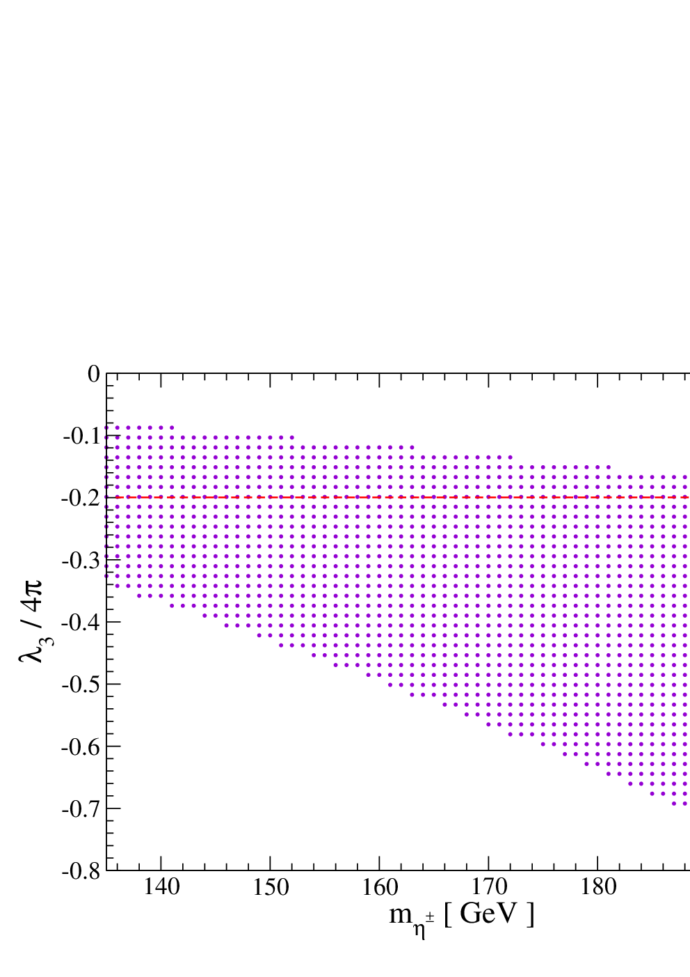
So, if the charged inert scalar $\eta^{+}$ is relatively light and $\lambda_{3}$ is negative and large, the observed excess $1.6\pm 0.4$ in the CMS experiment [26] can be explained. (The best-fit signal strength for this mode in the ATLAS experiment [25, 27] is $\hat{\mu}=1.9\pm 0.5$.) In Fig. 3 we show the area in the $m_{\eta^{\pm}}$–$\lambda_{3}$ plane in which $\Gamma(\gamma\gamma)/\Gamma^{\rm SM}(\gamma\gamma)=1.6\pm 0.4$ can be obtained ⁵⁵ 5 The upper bound $m_{\eta^{\pm}}<135$ GeV given in Ref. [31] is obtained from $\Gamma(\gamma\gamma)/\Gamma^{\rm SM}(\gamma\gamma)>1.3$ and $\lambda_{3}/4\pi>-1.46/4\pi\simeq-0.116$, which is consistent with Eq. (III.1). Note that we use $2.0\geq\Gamma(\gamma\gamma)/\Gamma^{\rm SM}(\gamma\gamma)\geq 1.2$ for Fig. 3 along with the stability constraint [Eq. (18)].. As we can see from Eq. (12), a large negative $\lambda_{3}$ may endanger the vacuum stability, because $\lambda_{1}$ is fixed at $0.129$. Therefore, we assume that all the quartic scalar couplings except $\lambda_{3}$ and $\lambda_{4}$ are positive and use the second set of the inequality conditions in Eqs. (16) and (17). Equation (18) means that $\lambda_{3}\mathrel{\mathchoice{\vbox{\halign{$\m@th\displaystyle\hfil#\hfil$\cr>\crcr\sim\crcr}}}{\vbox{\halign{$\m@th\textstyle\hfil#\hfil$\cr>\crcr\sim\crcr}}}{\vbox{\halign{$\m@th\scriptstyle\hfil#\hfil$\cr>\crcr\sim\crcr}}}{\vbox{\halign{$\m@th\scriptscriptstyle\hfil#\hfil$\cr>\crcr\sim\crcr}}}}-2.5$ if $\lambda_{2}$ is at the border of perturbation theory. Thus, the Higgs boson decay mode $h\to\gamma\gamma$ prefers the parameter space:

1. 1.

   All the quartic scalar couplings except $\lambda_{3}$ and $\lambda_{4}$ are positive, and $\lambda_{2}$ is large.

2. 2.

   The constraints

   $\displaystyle-0.2\mathrel{\mathchoice{\vbox{\halign{$\m@th\displaystyle\hfil#\hfil$\cr<\crcr\sim\crcr}}}{\vbox{\halign{$\m@th\textstyle\hfil#\hfil$\cr<\crcr\sim\crcr}}}{\vbox{\halign{$\m@th\scriptstyle\hfil#\hfil$\cr<\crcr\sim\crcr}}}{\vbox{\halign{$\m@th\scriptscriptstyle\hfil#\hfil$\cr<\crcr\sim\crcr}}}}\lambda_{3}/4\pi\mathrel{\mathchoice{\vbox{\halign{$\m@th\displaystyle\hfil#\hfil$\cr<\crcr\sim\crcr}}}{\vbox{\halign{$\m@th\textstyle\hfil#\hfil$\cr<\crcr\sim\crcr}}}{\vbox{\halign{$\m@th\scriptstyle\hfil#\hfil$\cr<\crcr\sim\crcr}}}{\vbox{\halign{$\m@th\scriptscriptstyle\hfil#\hfil$\cr<\crcr\sim\crcr}}}}-0.08~\mbox{and}~m_{\eta^{\pm}}\mathrel{\mathchoice{\vbox{\halign{$\m@th\displaystyle\hfil#\hfil$\cr<\crcr\sim\crcr}}}{\vbox{\halign{$\m@th\textstyle\hfil#\hfil$\cr<\crcr\sim\crcr}}}{\vbox{\halign{$\m@th\scriptstyle\hfil#\hfil$\cr<\crcr\sim\crcr}}}{\vbox{\halign{$\m@th\scriptscriptstyle\hfil#\hfil$\cr<\crcr\sim\crcr}}}}200~\mbox{GeV}~$

   have to be satisfied.

As we can see from Table I, either $N_{R}^{c}$ or $\eta$ can be a DM candidate. Here we assume that $\eta_{R}^{0}$, the CP-even component of $\eta$, is a DM particle and assume that $M_{k}\gg m_{\eta_{R}^{0}},~m_{\eta_{I}^{0}},~m_{\eta^{\pm}}$ to satisfy the $\mu\to e\gamma$ constraint [Eq. (II.3)]. The model can have three stable DM particles in principle, but to simplify the situation we assume a two-component DM system. Another one is either $\chi$ or $\phi$. As we see from the potential [Eq. (3)], there is no significant difference between $\chi$ and $\phi$ as DM. So we assume here that $\chi$ is the second DM particle.

The spin-independent elastic cross sections off the nucleon, $\sigma(\chi)$ and $\sigma(\eta^{0}_{R})$, are given by [59]:

where $\lambda_{L}=\lambda_{3}+\lambda_{4}$, $m_{N}$ is the nucleon mass, and $\hat{f}\sim 0.3$ stems from the nucleonic matrix element [60]. The cross sections have to satisfy

where $\Omega_{T}h^{2}=0.116$ [61], and $\sigma_{\rm UB}(m)\simeq 3\times 10^{-45}~\mbox{cm}^{2}$ [62] is the XENON100 limit for the DM mass of $135$ GeV. So, we find

where we would obtain the numbers in the parentheses when the XENON1T sensitivity $\sigma\sim 2\times 10^{-47}~\mbox{cm}^{2}$ [63] has been reached. Because of Eq. (2), we have to assume a large negative $\lambda_{3}$ and, because of $m^{2}_{\eta^{\pm}}-m^{2}_{\eta_{R}^{0}}=-\lambda_{4}v_{h}^{2}/2$, $\lambda_{4}$ has to be negative, too, to ensure $m_{\eta^{\pm}}>m_{\eta_{R}^{0}}$. If $\lambda_{4}$ is negative and in addition $\lambda_{3}$ is large and negative, the inequality of Eq. (16) may be violated, unless $\lambda_{4}$ is small and negative. This means $\lambda_{L}\simeq\lambda_{3}$, implying that Eq. (III.2) cannot be satisfied. Therefore, the relic density of $\eta_{R}^{0}$ has to be small to satisfy the constraint of Eq. (III.2). This is welcome, because the annihilation cross section of $\eta_{R}^{0}$ is large in general due to the gauge interactions shown in Fig. 4 [22, 23, 24]. Thus, the parameter space is further constrained:

1. 1.

   $\lambda_{4}$ has to be negative and small to ensure $m_{\eta^{\pm}}>m_{\eta_{R}^{0}}$ and to satisfy the constraint of Eq. (18).

2. 2.

   Since $\lambda_{3}$ is assumed to be large and negative [ see Eq. (2) ], the constraint of Eq. (III.2) can be satisfied only if $\Omega_{\eta}/\Omega_{T}\ll 1$.

3. 3.

   To satisfy the XENON100 (1T) constraint, we have to impose $|\gamma_{2}|\mathrel{\mathchoice{\vbox{\halign{$\m@th\displaystyle\hfil#\hfil$\cr<\crcr\sim\crcr}}}{\vbox{\halign{$\m@th\textstyle\hfil#\hfil$\cr<\crcr\sim\crcr}}}{\vbox{\halign{$\m@th\scriptstyle\hfil#\hfil$\cr<\crcr\sim\crcr}}}{\vbox{\halign{$\m@th\scriptscriptstyle\hfil#\hfil$\cr<\crcr\sim\crcr}}}}0.035(0.003)$ for $m_{\chi}=135$ GeV.

Since our parameter space has already been constrained to a certain amount, we next calculate the relic density of DM, $\Omega_{T}=\Omega_{\chi}+\Omega_{\eta}$. To simplify the situation we have been assuming throughout that $\eta_{R}^{0}$ and $\chi$ are DM particles. In this two-component DM system there are three different thermally averaged cross sections

that are relevant for calculating the DM relic density, where SM stands for the SM particles⁶⁶ 6 These thermally averaged cross sections are tree-level ones and do not include those into two $\gamma$’s. Annihilations into two $\gamma$’s will be separately calculated later on.. No semiannihilation $\eta_{R}^{0}\chi\to\phi_{R(I)}\mbox{SM}$ is allowed if $m_{\phi_{R(I)}}>m_{\eta_{R}^{0}}+m_{\chi}$. Then the evolution equation for $Y$, the number density over the entropy density, can be written as [18, 19, 20, 21]

where $\bar{Y}$ is $Y$ in equilibrium, $x=\mu/T$, $1/\mu=1/m_{\eta_{R}^{0}}+1/m_{\chi}$, and $T,M_{\rm PL}$ and $g_{*}=90$ are the temperature, the Planck mass and the total number of effective degrees of freedom, respectively.

Before we solve the evolution equations numerically, we consider what we would expect. As noticed, the relic density of $\eta_{R}^{0}$ will be very small because of large $\lambda_{3}$ and gauge interactions (i.e. large $\langle\sigma(\eta_{R}^{0}\eta_{R}^{0};\mbox{SM})v\rangle$), while the annihilation cross section of $\chi$ into the SM particles is suppressed because of Eq. (III.2) (i.e. small $\langle\sigma(\chi\chi;\mbox{SM})v\rangle$). That is, the DM conversion cross section $\langle\sigma(\eta_{R}^{0}\eta_{R}^{0};\chi\chi)v\rangle$ and the mass difference $\Delta m_{\eta\chi}=m_{\eta_{R}^{0}}-m_{\chi}$ will play an important role. Note that the smaller $\Delta m_{\eta\chi}$ is, the larger is the effect of the DM conversion on $\Omega_{\chi}$. To see this more explicitly, we assume that $\eta_{R}^{0}$ annihilates very fast so that before and at the decoupling of $\chi$ the $\eta_{R}^{0}$ DM is in thermal equilibrium. Then the expression in $\{~\}$ in the rhs of Eq. (103) can be written as

which also appears in the coannihilation of DM with an unstable particle [50] ⁷⁷ 7 The mechanism has been also used in the model of Refs. [51, 45], explaining the monochromatic $\gamma$ at the Fermi LAT. But the light charged scalar faces a problem in explaining the neutrino mass.. If $m^{2}_{\chi}-m^{2}_{\eta_{R}^{0}}<0$, the effective annihilation cross section of $\chi$ is small at low temperature (large $x$), while it is large at high temperature (small $x$). Because of the nontrivial interplay between $\gamma_{2}$ and $\Delta m_{\eta\chi}$, it may be possible to obtain a correct relic density $\Omega_{T}h^{2}=0.1157\pm 0.0023$ [61]. In Fig. 5 we show the effective annihilation cross section [ the expression in [ ] of Eq. (104) ] as a function of $x=\mu/T$ for $m_{\eta_{R}^{0}}=148$ (dotted), $153$ (solid), and $156$ (dashed) GeV, where we have fixed the parameters as

As we see from Fig. 5 the effective cross section around the decoupling temperature $x\sim 20$ has a correct size and decreases drastically at low temperature. The effective cross section is normalized to $10^{-26}~\mbox{cm}^{3}\mbox{s}^{-1}$, because it is the size to obtain the observed relic density of DM. The scalar couplings $\lambda_{2},\gamma_{1}$ and $\gamma_{4}$ do not enter into the cross sections [ Eq. (101) ], and $\gamma_{5},\gamma_{6},\gamma_{7}$ and $\kappa$ are irrelevant because $\phi$ is much heavier than $\eta$ and $\chi$.

In Fig. 6 we show the area in the $\gamma_{2}$–$\gamma_{3}$ plane in which the total relic density $\Omega_{T}h^{2}=0.1157\pm 0.0046~(2\sigma)$ with $m_{\chi}=135$ GeV can be obtained for $m_{\eta_{R}^{0}}=148~(\mbox{red})$, $152~(\mbox{green})$, $153~(\mbox{blue})$, $153.3~(\mbox{cyan})$, $153.5~(\mbox{purple})$, $154~(\mbox{yellow})$ and $156~(\mbox{black})$ GeV. The right-handed neutrino masses, $M_{k}$, are all $1$ TeV, and the Yukawa couplings are chosen to yield $\sum_{ik}|Y^{\nu}_{ik}|^{2}=(10^{-4})^{2}$. The vertical (black dashed) lines are the upper bounds of $\gamma_{2}$ set by the XENON 100 (right) and 1T (left) experiments [Eq. (III.2) ]. From Fig. 6 we can also see that there exists a parameter space with $m_{\chi}=135$ GeV, $m_{\eta_{R}^{0}}>153$ GeV, a large $\gamma_{3}/4\pi$ (between $0.65$ and $1.0$) and $\gamma_{2}$ satisfying the XENON constraint [Eq. (III.2) ]. A large $\gamma_{3}$ is needed to explain the $135$ GeV $\gamma$-ray line in the Fermi spectrum, as we will see below.

Our model contains the coupling between $\chi$ and $\eta^{+}$ (${\cal L}_{\eta^{\dagger}\eta\chi^{2}}=-\gamma_{3}~\eta^{\dagger}\eta\chi^{2}$). Because of this coupling there are diagrams in Fig. 7, which produce monochromatic $\gamma$ lines through the annihilation of $\chi$. We would like to use these diagrams to explain the monochromatic $\gamma$-ray line [36, 37, 40, 41] observed at the Fermi LAT [32, 33, 34, 35]. There exist also s-channel diagrams with the SM Higgs propagator as shown in Fig. 8. The $h\chi\chi$ coupling is proportional to $\gamma_{2}$, while $h\eta_{R}^{0}\eta_{R}^{0}$ coupling is proportional to $\lambda_{3}$. The annihilation cross section $\sigma(\eta_{R}^{0}\eta_{R}^{0}\to\gamma\gamma)$ is large, because $\lambda_{3}$ is large [see Eqs. (III.1) and (2)] ⁸⁸ 8 In [42], $\sigma(\eta_{R}^{0}\eta_{R}^{0}\to\gamma\gamma)$ is used to explain the monochromatic $\gamma$-ray line, where a fine-tuned cancellation mechanism to suppress the total annihilation cross section of $\eta_{R}^{0}$ [24] is employed . Besides, due to the gauge interactions (see the right diagram of Fig. 4) the relic density of $\eta_{R}^{0}$ is very small, so the annihilation of the $\eta_{R}^{0}$ DM cannot contribute to the monochromatic $\gamma$-ray. Furthermore, for the same reason, the tree-level annihilations of $\eta_{R}^{0}$ into a pair of $W$’s and $Z$’s, which would contribute to the continuum $\gamma$-ray spectrum, are also suppressed. In contrast to this case, the pure gauge interaction (the right diagram of Fig. 4) is absent for the annihilation of $\chi$. The entire annihilations of $\chi$ into the SM particles are controlled by the single coupling $\gamma_{2}$, which has to satisfy the constraint of Eq. (III.2). Therefore, we may assume that the main contribution to $\sigma(\chi\chi\to\gamma\gamma)$ comes from the one-loop diagrams in Fig. 7 and find

References

- [1] P. Minkowski, Phys. Lett. B 67 (1977) 421.
- [2] M. Gell-Mann, P. Ramond, and R. Slansky, in Supergravity, eds. P. van Nieuwenhuizen and D. Z. Freedman (North-Holland, 1979), p. 315; T. Yanagida, in Proc. of the Workshop on the Unified Theory and the Baryon Number in the Universe, eds. O. Sawada and A. Sugamoto, KEK Report No. 79-18 (Tsukuba, Japan, 1979), p. 95.
- [3] R. N. Mohapatra and G. Senjanovic, Phys. Rev. Lett. 44 (1980) 912.
- [4] A. Zee, Phys. Lett. B 93 (1980) 389 [Erratum-ibid. B 95 (1980) 461].
- [5] A. Zee, Nucl. Phys. B 264 (1986) 99.
- [6] K. S. Babu, Phys. Lett. B 203 (1988) 132.
- [7] L. M. Krauss, S. Nasri and M. Trodden, Phys. Rev. D 67 (2003) 085002 [hep-ph/0210389].
- [8] E. Ma, Phys. Rev. D 73 (2006) 077301 [hep-ph/0601225].
- [9] K. Cheung and O. Seto, Phys. Rev. D 69 (2004) 113009 [hep-ph/0403003].
- [10] J. Kubo, E. Ma and D. Suematsu, Phys. Lett. B 642 (2006) 18 [hep-ph/0604114].
- [11] M. Aoki, S. Kanemura and O. Seto, Phys. Rev. Lett. 102 (2009) 051805 [arXiv:0807.0361 [hep-ph]]; Phys. Rev. D 80 (2009) 033007 [arXiv:0904.3829 [hep-ph]].
- [12] F. Bonnet, M. Hirsch, T. Ota and W. Winter, JHEP 1207 (2012) 153 [arXiv:1204.5862 [hep-ph]].
- [13] Y. Farzan, S. Pascoli and M. A. Schmidt, JHEP 1303 (2013) 107 [arXiv:1208.2732 [hep-ph]].
- [14] S. Kanemura and T. Ota, Phys. Lett. B 694 (2010) 233 [arXiv:1009.3845 [hep-ph]].
- [15] S. Kanemura, T. Nabeshima and H. Sugiyama, Phys. Lett. B 703 (2011) 66 [arXiv:1106.2480 [hep-ph]].
- [16] S. S. C. Law and K. L. McDonald, Phys. Lett. B 713 (2012) 490 [arXiv:1204.2529 [hep-ph]].
- [17] G. Guo, X. -G. He and G. -N. Li, JHEP 1210 (2012) 044 [arXiv:1207.6308 [hep-ph]].
- [18] F. D’Eramo and J. Thaler, JHEP 1006 (2010) 109 [arXiv:1003.5912 [hep-ph]].
- [19] G. Belanger and J.-C. Park, JCAP 1203 (2012) 038 [arXiv:1112.4491 [hep-ph]].
- [20] G. Belanger, K. Kannike, A. Pukhov and M. Raidal, JCAP 1204 (2012) 010 [arXiv:1202.2962 [hep-ph]].
- [21] M. Aoki, M. Duerr, J. Kubo and H. Takano, Phys. Rev. D 86 (2012) 076015 [arXiv:1207.3318 [hep-ph]].
- [22] L. Lopez Honorez, E. Nezri, J. F. Oliver and M. H. G. Tytgat, JCAP 0702 (2007) 028 [arXiv:hep-ph/0612275].
- [23] E. M. Dolle and S. Su, Phys. Rev. D 80 (2009) 055012 [arXiv:0906.1609 [hep-ph]].
- [24] L. Lopez Honorez and C. E. Yaguna, JCAP 1101 (2011) 002 [arXiv:1011.1411 [hep-ph]].
- [25] G. Aad et al. [ATLAS Collaboration], Phys. Lett. B 716 (2012) 1 [arXiv:1207.7214 [hep-ex]].
- [26] S. Chatrchyan et al. [CMS Collaboration], Phys. Lett. B 716 (2012) 30 [arXiv:1207.7235 [hep-ex]].
- [27] ATLAS Collaboration, ATLAS-CONF-2012-091.
- [28] J. F. Gunion, H. E. Haber, G. L. Kane and S. Dawson, Front. Phys. 80 (2000) 1.
- [29] A. G. Akeroyd, M. A. Diaz and M. A. Rivera, Phys. Rev. D 76 (2007) 115012 [arXiv:0708.1939 [hep-ph]].
- [30] A. Arhrib, R. Benbrik and N. Gaur, Phys. Rev. D 85 (2012) 095021 [arXiv:1201.2644 [hep-ph]].
- [31] B. Swiezewska and M. Krawczyk, arXiv:1212.4100 [hep-ph].
- [32] W. B. Atwood et al. [LAT Collaboration], Astrophys. J. 697 (2009) 1071 [arXiv:0902.1089 [astro-ph.IM]].
- [33] A. A. Abdo, M. Ackermann, M. Ajello, W. B. Atwood, L. Baldini, J. Ballet, G. Barbiellini and D. Bastieri et al., Phys. Rev. Lett. 104 (2010) 091302 [arXiv:1001.4836 [astro-ph.HE]].
- [34] M. Ackermann et al. [LAT Collaboration], Phys. Rev. D 86 (2012) 022002 [arXiv:1205.2739 [astro-ph.HE]].
- [35]
Fermi-LAT Collaboration,
http://fermi.gsfc.nasa.gov/science/mtgs/symposia
/2012/program/fri/AAlbert.pdf - [36] T. Bringmann, X. Huang, A. Ibarra, S. Vogl and C. Weniger, JCAP 1207 (2012) 054 [arXiv:1203.1312 [hep-ph]].
- [37] C. Weniger, JCAP 1208 (2012) 007 [arXiv:1204.2797 [hep-ph]].
- [38] E. Tempel, A. Hektor and M. Raidal, JCAP 1209, 032 (2012) [Addendum-ibid. 1211, A01 (2012)] [arXiv:1205.1045 [hep-ph]].
- [39] A. Rajaraman, T. M. P. Tait and D. Whiteson, JCAP 1209 (2012) 003 [arXiv:1205.4723 [hep-ph]].
- [40] M. Su and D. P. Finkbeiner, arXiv:1206.1616 [astro-ph.HE].
- [41] M. Su and D. P. Finkbeiner, arXiv:1207.7060 [astro-ph.HE].
- [42] A. Biswas, D. Majumdar, A. Sil and P. Bhattacharjee, arXiv:1301.3668 [hep-ph].
- [43] F. D’Eramo, M. McCullough and J. Thaler, JCAP 1304 (2013) 030 [arXiv:1210.7817 [hep-ph]].
- [44] P. -H. Gu, arXiv:1301.4368 [hep-ph].
- [45] S. Baek, P. Ko and E. Senaha, arXiv:1209.1685 [hep-ph].
- [46] Y. Bai, V. Barger, L. L. Everett and G. Shaughnessy, arXiv:1212.5604 [hep-ph].
- [47] J. M. Cline, Phys. Rev. D 86 (2012) 015016 [arXiv:1205.2688 [hep-ph]].
- [48] L. Wang and X. -F. Han, Phys. Rev. D 87 (2013) 015015 [arXiv:1209.0376 [hep-ph]].
- [49] J. Fan and M. Reece, arXiv:1301.2597 [hep-ph].
- [50] K. Griest, D. Seckel, Phys. Rev. D43 (1991) 3191-3203.
- [51] S. Tulin, H. -B. Yu, K. M. Zurek and , Phys. Rev. D 87 (2013) 036011 [arXiv:1208.0009 [hep-ph]].
- [52] E. Ma, Phys. Lett. B 659 (2008) 885 [arXiv:0710.2325 [hep-ph]].
- [53] W. A. Bardeen, FERMILAB-CONF-95-391-T.
- [54] H. Aoki, S. Iso and , Phys. Rev. D 86 (2012) 013001 [arXiv:1201.0857 [hep-ph]].
- [55] G. Passarino and M. J. G. Veltman, Nucl. Phys. B 160, 151 (1979).
- [56] E. Ma and M. Raidal, Phys. Rev. Lett. 87 (2001) 011802 [Erratum-ibid. 87 (2001) 159901] [arXiv:hep-ph/0102255].
- [57] K. Hayasaka, arXiv:1010.3746 [hep-ex].
- [58] J. Beringer et al. [Particle Data Group Collaboration], Phys. Rev. D 86 (2012) 010001.
- [59] R. Barbieri, L. J. Hall and V. S. Rychkov, Phys. Rev. D 74 (2006) 015007 [arXiv:hep-ph/0603188].
- [60] J. R. Ellis, A. Ferstl and K. A. Olive, Phys. Lett. B 481 (2000) 304 [arXiv:hep-ph/0001005].
- [61] G. Hinshaw, D. Larson, E. Komatsu, D. N. Spergel, C. L. Bennett, J. Dunkley, M. R. Nolta and M. Halpern et al., arXiv:1212.5226 [astro-ph.CO].
- [62] E. Aprile et al. [XENON100 Collaboration], Phys. Rev. Lett. 109 (2012) 181301 [arXiv:1207.5988 [astro-ph.CO]].
- [63] E. Aprile [XENON1T Collaboration], arXiv:1206.6288 [astro-ph.IM].
- [64] T. Cohen, M. Lisanti, T. R. Slatyer and J. G. Wacker, JHEP 1210 (2012) 134 [arXiv:1207.0800 [hep-ph]].
- [65] W. Buchmuller and M. Garny, JCAP 1208 (2012) 035 [arXiv:1206.7056 [hep-ph]].
- [66] G. Belanger, C. Boehm, M. Cirelli, J. Da Silva and A. Pukhov, JCAP 1211, 028 (2012) [arXiv:1208.5009 [hep-ph]].
- [67] O. Adriani et al. [PAMELA Collaboration], Phys. Rev. Lett. 105 (2010) 121101 [arXiv:1007.0821 [astro-ph.HE]].
- [68] A. Ibarra and D. Tran, JCAP 0807 (2008) 002 [arXiv:0804.4596 [astro-ph]].
- [69] F. Donato, D. Maurin, P. Brun, T. Delahaye and P. Salati, Phys. Rev. Lett. 102 (2009) 071301 [arXiv:0810.5292 [astro-ph]].
- [70] W. Buchmuller, A. Ibarra, T. Shindou, F. Takayama and D. Tran, JCAP 0909 (2009) 021 [arXiv:0906.1187 [hep-ph]].
- [71] M. Asano, T. Bringmann, G. Sigl and M. Vollmann, Phys. Rev. D 87 (2013) 103509 [arXiv:1211.6739 [hep-ph]].
- [72] D. Whiteson, arXiv:1302.0427 [astro-ph.HE].
- [73] C. Weniger, arXiv:1303.1798 [astro-ph.HE].