A Constructive Method for Approximate Solution to Scalar Wiener-Hopf Equations
Abstract.
This paper presents a novel method of approximating the scalar Wiener-Hopf equation; and therefore constructing an approximate solution. The advantages of this method over the existing methods are reliability and explicit error bounds. Additionally the degrees of the polynomials in the rational approximation are considerably smaller than in other approaches.
The need for a numerical solution is motivated by difficulties in computation of the exact solution. The approximation developed in this paper is with a view of generalisation to matrix Wiener-Hopf for which the exact solution, in general, is not known.
The first part of the paper develops error bounds in for . These indicate how accurately the solution is approximated in terms of how accurate the equation is approximated.
The second part of the paper describes the approach of approximately solving the Wiener-Hopf equation that employs the Rational Carathéodory-Fejér Approximation. The method is adapted by constructing a mapping of the real line to the unit interval. Numerical examples to demonstrate the use of the proposed technique are included (performed on Chebfun), yielding error as small as on the whole real line.
Key words and phrases:
Wiener-Hopf, Riemann-Hilbert, rational approximation, Rational Carathéodory-Fejér Approximation, Chebfun, constructive1. Introduction
The Wiener-Hopf method is used for a broad collection of PDEs which arise in acoustic, finance, hydrodynamic, elasticity, potential and electromagnetic theories [15, 2]. It is an elegant method based on the exploitation of the analyticity properties of the functions. For the scalar Wiener-Hopf the solution can be expressed in terms of a Cauchy type integral [16]*Ch. 1.3.
In more complicated scalar Wiener-Hopf equations the exact solution is difficult or slow to compute, see e.g. [1, 23, 14]. Approximate solutions were considered early on but they were mainly constructed using ad hoc observations [16]*Ch. 4.5. In 2000 a systematic way of approximating the Wiener-Hopf equations was published by I. D. Abrahams [3]. Since then it proved popular and found applications in different branches of mathematics including finance [10].
The method proposed in [3] is based on uniform approximations of the kernel on the whole strip by a two point Padé approximation (the two points being 0 and on the real axis). However, there are two issues that make the application of this method difficult. The first is that it is unclear when the two point Padé approximation has small error on the whole strip [6]. Secondly, even if the maximum error of approximating the kernel on the whole strip is known, there are no error bounds presented to calculate the resulting error in the solution.
Another motivation for the development of approximate methods is the matrix Wiener-Hopf problem. The determination of a good numerical solution is important for the matrix Wiener-Hopf problem, since as yet there is no constructive way of solving it in general.
This paper aims to present a consistent method of approximately solving the scalar Wiener-Hopf. The following questions are addressed:
Problem 1.
Given a scalar Wiener-Hopf problem find an approximate solution which can be demonstrated to be within a given accuracy from the exact solution.
Problem 2.
How to perform Problem computationally in a way that is reliable, optimal and easy.
Problem will be addressed in Section with new estimations for the error in the Wiener-Hopf factors. This is done though expressing the factors in terms of the Hilbert transform, which is connected to the Cauchy singular integral. Note that although the method proposed in this paper involves the construction of an approximate solution to the given Wiener-Hopf equation, the solution is the exact solution of a perturbed Wiener-Hopf equation.
The main difficulty in Problem is that the Wiener-Hopf equation is set on an unbounded interval. We propose the novel method based on an appropriate mapping to the unit interval, see Section . This allows the Carathéodory-Fejér rational approximation to then be used in Section . Lastly, numerical examples are given.
2. Preliminaries
The following conventions will be used throughout the paper. A strip around the real axis (given ) is { : }. The subscript (or ) indicates that the function is analytic in the half-plane (or ). Functions in the Wiener-Hopf equation without the subscript are analytic in the strip.
The Wiener-Hopf problems are recalled below.
The multiplicative Wiener-Hopf problem is: given a function (analytic, zero-free and as in the strip) to find functions and which satisfy the following equation in the strip:
| (2.1) |
In addition and are required to be:
- •
analytic and non-zero in the respective half-plane.
- •
of subexponential growth the respective half-planes:
The function in the multiplicative Wiener-Hopf factorisation will be referred to as the kernel. The functions and will be called factors of . Those factor are unique up to a constant. In other words if there are two such factorisations and then:
where is an arbitrary complex number [13]. In this paper they will be normalised so that as in the strip.
Remark 2.1.
The above normalisation at infinity allows to control the regularity of the Fourier transform of an approximation. This is useful if a factorisation of the Fourier transform is used, say, for a solution of differential equations.
The multiplicative Wiener-Hopf factorisation can be reduced to the additive Wiener-Hopf problem via application of logarithm. Under the conditions on the kernel , let then additive Wiener-Hopf problem is: given a function to find functions and which satisfy the following equation in the strip:
| (2.2) |
Additive and multiplicative problems are equivalent only in the scalar case. In the matrix Wiener-Hopf and will in general not be commutative so no such equivalence is possible.
The existence of solutions to the additive and multiplicative scalar Wiener-Hopf problem is addressed in for example [16]*Ch. 1.3.
These two Wiener-Hopf splittings are key to solving the general Wiener-Hopf problem. That is: given functions and find functions and , which satisfy the following equation in the strip:
| (2.3) |
For more details about the Wiener-Hopf problem see [16].
2.1. The Riemann-Hilbert Problem
The Wiener-Hopf problem is a special case of the Riemann-Hilbert problem. Roughly, the Riemann-Hilbert problem has a more general contour instead of the strip and the conditions on the function are weakened. In particular it is required that is only Hölder continuous on the contour.
Let be Hölder continuous functions on a simple contour . The Riemann-Hilbert problem is to find an analytic function which has values on the contour as the limit is taken from different sides of the contour and which satisfies the equation:
The Wiener-Hopf equation (2.3) can be considered as the special case of the Riemann-Hilbert problem so a good approximation of the values of the function on the real line is sufficient. This is simpler than trying to construct an approximation that agrees well on the whole strip of analyticity.
3. Estimates on the Approximate Wiener-Hopf Factorisation
The approximate solution to (2.1) can be found by approximating the kernel in the Wiener-Hopf equation. This section quantifies the difference between the modified and the original Wiener-Hopf equation, to address Problem introduced earlier. More precisely, let , the aim is to bound in terms of and computable quantities of .
The first step is to link the Wiener-Hopf factorisation to the Hilbert Transform of with . If:
then [17]*Ch. 2:
and hence:
The advantage of expressing in terms of the Hilbert transform is the following theorem.
Theorem 3.1 (Titchmarsh-Riesz).
Based on these classical estimations we obtain the following bounds on the additive Wiener-Hopf factorisation.
Proof.
Expressing in terms of the Hilbert transform and using Minkowski’s inequality:
Here the linearity property of the Hilbert transform, is used. ∎
The theorem gives bounds on the error on the real line but in fact since the functions are analytic, the bounds will hold in the upper/lower half-planes by the maximum modulus principle.
It will be useful to express the Wiener-Hopf factors in terms of the Hilbert transform;
The main new result of this section is:
Theorem 3.3 (Multiplicative Bounds in for ).
Let and be two kernels and . If then:
where is defined in (3.1).
Proof.
The first step is to express the product factorisation as an additive factorisation. Taking logarithms:
From the assumptions on the kernel , will be a continuous and single valued function and hence the additive decomposition is well defined. Given:
Then using the mean value inequality (and ):
Apply Lemma 3.2, which gives:
Lastly, note that since:
and so:
from which the result follows. ∎
Remark 3.4 (Real Kernels).
In the case when kernels and are real valued, the bounds could be simplified, since then and so:
Remark 3.5 ( norm).
The above theorem does not include the case of norm, in fact no such result is possible for the norm as is demonstrated by the counter example below.
Consider defined on the real line and
and
Then:
but it has been shown by making small the factors can differ by an arbitrary large amount in norm, see [5].
Below, the proposed method of the solution of Problem is presented:
- •
Approximate, with arbitrary accuracy, the Wiener-Hopf kernel by rational functions .
- •
Perform the Wiener-Hopf factorisation of the rational kernel by inspection. The will have the form:
where the () are all the zeroes (poles) of which lie in the lower half-plane. The other factor will have the remainder poles and zeroes in the upper half-plane.
- •
Using Theorem 3.3 the error can be calculated.
The rest of the paper will concentrate on Problem 2 i.e. the practical aspect of Problem 1.
4. Mapping of the Real Line
In the previous section it was proved that the approximation of the kernel results in a computable error in the Wiener-Hopf factors. Thus, to simplify the problem one may wish to approximate a kernel by another which is easier to factorise e.g. by rational functions. To construct such an approximation the first step is to employ a mapping of the real line to the unit circle or the interval . Those mappings transform the problem of approximation on the whole real line to a simpler problem on the unit circle or the interval. Methods for approximating on the unit circle and the interval will be discussed in the next section.
To easily distinguish between functions defined on the real axis, the unit circle, and the interval the following notation will be fixed:
- •
Functions on the real line will be denoted by capital letter and variable , for example ;
- •
Functions on the unit circle will be denoted by small case letter and variable , for example ;
- •
Functions on the interval will be denoted by bold capital letters and variable , for example ;
- •
The rational approximation for functions will be denoted by letters with a tilde, for example
It is typical in applications for the kernel to be an even function (i.e. ) and the mapping is simplified in this case. Therefore it is instructive to consider the mapping for even functions before considering the general case.
4.1. Even Functions
Define a conformal Möbious map that maps the real line to the unit circle as follows [7]*Ch 13:
Explicitly it is given by:
The next map is a projection of the unit circle to the interval by the Joukowski map (a conformal map which, incidentally, comes from aerodynamics [19]). The Joukowski map is:
| (4.1) |
Restricted to the unit circle the map returns the real part of . This step requires the function to be even. Even functions will be mapped to a function on the unit circle with the property . Composing these maps together:
This enables the construction of a function on the interval from a given function on the real line as follows:
Then the algorithm of the next section can be used to rationally approximate on by . Suppose that the error in this approximation in the is .
Then map the function back to the real line by:
Furthermore is a rational function on the real line that approximates on the real line with the error at most .
The maps described above are combined with the Carathéodory-Fejér algorithm in Chebfun to give the code used for the numerical examples in the next section.
Remark 4.1.
If the kernel is odd i.e. the kernel can be squared to produce an even kernel. Then the approximation can be produced as above and square rooted. Note that the explicit multiplicative Wiener-Hopf factorisation of the square root of a rational function is done by inspection in the same way as for the rational function. Also note that any function can be written as a sum of even and odd function, thus the above extends to a general function.
4.2. General Functions
For a general kernel the above map can be modified. The above method contains the following ideas. The real line is conformally mapped to the circle. Then only half of the circle is mapped to the interval ; however this poses no problem since the other half is the same due to the function being even. The function is approximated and mapped back to the unit circle. The modification is needed to ensure that half of the function is not discarded. Thus, after mapping the real line to the circle, apply the map ; this makes the values run twice as fast and the whole function now fits on the half circle. Next, as before, map this half circle to the interval, approximate, and map back. The values that are taken on the half circle are spread out to the circle by the map .

Remark 4.2.
Before using a map it is beneficial to apply a rescaling and a shift (i.e. Möbious map) to the real line so that the part of the function which has a fast changing gradient fits in the interval . This part of the real line is well resolved, see Figure 1.
4.3. Associated Orthogonal Rational Functions
In this section the properties of the map (4.2) will be studied. This will be done by considering the new basis functions which are created by this map. A starting point is to choose a basis function for the circle; a good choice for this is the Fourier basis. Then the Joukowski map will create the new basis for the interval as the image of the Fourier basis, under the change of coordinates, [9]*Sec 1.6. This new basis is the Chebyshev polynomials of the first kind (they are also the Fabe polynomials on up to a multiplicative factor [18]). Furthermore, the mapping from to will create a new basis (from Chebyshev polynomials) called Rational Chebyshev Functions, [8]. They are defined as:
where the are the Chebyshev polynomials of the first kind and is the map , see (4.2). Note that, despite the name, are not all rational: the are rational functions divided by (the are all rational function).
A useful property of is the shape of the domain of convergence. This is especially informative when the kernel has no singularities on the whole real line including infinity. For standard basis functions the domain of convergence has a specific shape and the size is determined by the position of singularities [8]. For example, Taylor series converge on a circle and Chebyshev series converge on an ellipse, the sizes of which are dictated by the position of the singularities. The shape of the domain for is the exterior of two circles which are the image of lines parallel to the real axis under the Möbious map . This is derived from the corresponding domain of convergence for Chebyshev polynomials which in turn comes from the Fourier series [8].
So in particular those base functions are well suited for functions which have singularities in the bounded part of the complex plane, like Example 6.1. This compares favourably to the domain of convergence of Taylor expansion for a function like the one in Example 6.1. In particular, this explains why all methods of approximation which are based on the Taylor expansion do not produce good results on the whole real line (e.g. one point Padé approximation).
For functions with a singularity at infinity the following theorem by Boyd is applicable.
Theorem 4.3 (Convergence of the Fourier series for an algebraically decaying or asymptotically constant function).
[8, Sec 5] If a function is free from singularities on the real axis and has the inverse power expansion
| (4.3) |
as and a similar series as , then the coefficients of its representation as a Fourier series in the new coordinate (where and , see (4.2)),
| (4.4) |
will have exponential convergence in the sense that and decrease with n faster than any finite inverse power of .
Remark 4.4.
The theorem covers precisely the class of functions that arises as kernels in the additive and multiplicative Wiener-Hopf factorisation. In the additive case the kernel must decrease faster than some power and in the multiplicative case they are asymptotically .
The above theorem shows one of the strengths of the compared to other base functions on an unbounded interval e.g. the Hermite and sinc functions. The latter only converge algebraically for algebraically decaying functions.
5. Rational Approximation
The best rational approximation in is not practical to use, see [22]. This section describes a near best method of rational approximation named AAK (Adamjan-Arov-Kreĭn) [4] in the general case and Rational Carathéodory-Fejér [11, 21] in the case of real valued functions. The AAK theory is briefly reviewed at the end. Unfortunately it seems that there is no software that performs AAK approximation; only software for Rational Carathéodory-Fejér have been developed that is Chebfun (MATLAB) [22].
5.1. Real Rational Approximation
Below a brief summary of the method from [20] is presented. Let be a real continuous function on . For any natural number , has a partial Chebyshev expansion:
where
and are Chebyshev polynomials of the first kind.
An application of the Joukowski map (see (4.1)) to produces an associated function on the unit circle:
The above is true because of the intimate connection of the Chebyshev polynomials and Joukowski transform given by:
Define:
where we are seeking a rational approximation. Next approximate on the unit circle by an extended rational function of the form:
| (5.1) |
where the numerator is a bounded analytic function in and the denominator has no zeroes in . Call a class of functions of the above form . Note that this is not a typical class to approximate by, but it is the one for which a neat solution exists. After the approximation (5.1) is obtained it can be truncated to get a rational approximation. To obtain an approximation in consider a real symmetric Hankel matrix:
Let be eigenvalues of arranged in decreasing order by magnitude of absolute value. And let be an eigenvector for the eigenvalue. Then the following theorem is true:
Theorem 5.1 (Takagi).
The analytic function has a unique best approximation on the unit circle in given by:
where is the finite Blaschke product
And the approximation error in norm on the unit circle is .
Once the approximation is obtained, it is mapped back from the unit circle to the unit interval by the inverse of the Joukowski transform. A subsequent truncation gives a near best rational approximation on the interval.
This is a fast and efficient way of computing rational approximations. Furthermore, it enables to predict the error on the approximation even before the approximation is computed by considering eigenvalues.
5.2. AAK Approximation
This section presents more general results to the ones covered in the previous section. These apply to complex valued functions on the unit circle and are taken from [4].
Definition 1.
Given a natural number , define a class of bounded functions on the unit circle which can be expressed as:
where is a rational function that has no more than poles all inside the unit circle and .
The AAK approximation solves the following problem:
Given a function and natural number, find the best approximation in the norm from functions in the .
In other words it is required to find:
and a function (if it exists) such that:
The solution to the above is presented in the next theorem.
Theorem 5.2.
[4] Let , then where is the Hankel matrix build out of Fourier coefficients of and is the singular value of it. Moreover,
where is a Schmidt pair for a Hankel matrix and where:
The next section illustrates theory with examples.
6. Numerical Examples
In this section the numerical examples are provided to illustrate the theory (performed in Chebfun, MATLAB).
6.1. Example 1a

The first example (see Figure 2) is
| (6.1) |
Take the finite branch cut from to and from to . This kernel is closely associated with the matrix kernel factorisation from problems in acoustics and elasticity and was studied by I. D Abrahams [3]. The case will be considered in the numerical examples. The first approach is to approximate this given function on an interval, a process called domain truncation. On the surface, the results look promising (see top Figure 3); the error decreases as the degree of the numerator polynomial is increased.
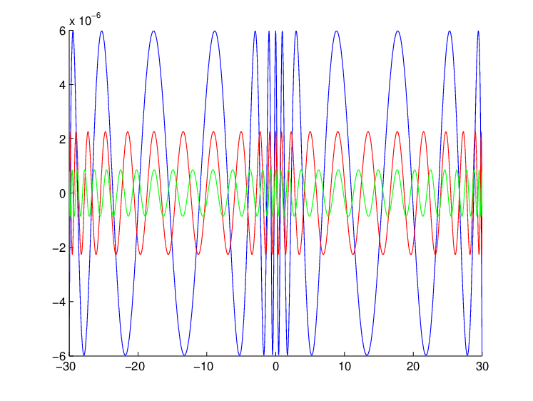

Nevertheless there are problems, the most obvious being that [20,4] or any other approximations plotted in top Figure 3 have very different behaviours at infinity than . The error will be small but only on the given interval and will not be controlled outside it. It might be tempting to try to rectify this, since will be zero outside a sufficiently large interval. One might suggest to look at approximations where is smaller than : this type of function will go to zero at infinity. But, although the error on most of the real axis is very small, just outside the interval it tends to be greater (and much larger than it is inside the interval). Another feature of this type of approximation is how the poles and zeroes are positioned. Although some of the poles are positioned on the branch cuts and , there are a lot of singularities introduced elsewhere (see bottom Figure 3).
In the next section, the mapping constructed in Section 4 will be used to overcome the described problems. This will also result in smaller degree of the polynomials.
6.2. Example 1b
The previous example (6.1) is treated with the mapping proposed in Section 4 for even functions. The function mapped to the interval becomes:

In Figure 4 the new function is plotted; notice that in this form it is much easier to approximate, since it has a slow changing gradient. This is confirmed by the error curve for the approximation; the error is of order . Furthermore, a better result is obtained with approximation with error of order (see Figure 5).


At this point the approximated function can be mapped back to the real line and the norm of the error will stay the same, see Figure 6 (solid curves). Note that it now becomes a [10,10] rational approximation. This example was chosen because the Wiener-Hopf factors can be easily seen by inspection. They are:
The factors of the rational approximation can be easily calculated and compared to the exact solution above; this is plotted in Figure 6 (dotted curve). This error is smaller than the error obtained in [3] even with for the same function.
What is more, the poles and zeroes also lie almost exactly on the branch cuts and . The close proximity of zeroes and poles mimic the behaviour of a branch cut. This indicates that the behaviour in the whole complex plane is correct (see Figure 7). Note that the scale of the -axis is .
Bounds developed for real-valued kernels in Section 3 could be applied to this example. The bounds will be used. Note , and this gives:
The norm is easy to estimate numerically in Chebfun by using the norm command. For the [10,10] rational approximation these calculations give:
which agrees with the bounds above.
6.3. Example 2
The function is (Figure 8):


This kernel is related to the one considered in Koiter’s paper of [12] and is typical for electrostatic and slow flow problems. In the original article, rational approximations were considered by choosing the coefficients by hand, accuracy of was achieved. Once again the function becomes easier to approximate (on the whole real line) once it is mapped to the interval , Figure 8. The mapped function is (the general mapping is used):
This can then be approximated with errors of (giving the graph similar to Figure 5) with even though the point at infinity is singular (it is an accumulation point of a sequence of poles). Interestingly, the position of zeroes and poles (see Figure 9) is very similar to that found in [3]*Fig 8 with a different method of approximating.

This kernel has exact factorisation which is given by:
But MATLAB does not have an inbuilt complex function hence the results of this approximation cannot be compared to the exact factorisation. Even if there was an inbuilt complex function to compare it to the approximate solution the inbuilt function would need to have very high accuracy. This demonstrate that if the numerical values of the solution is needed the approximate solution is as good as the exact solution.
7. Conclusion
This paper demonstrates with use of examples the method of approximate solution of the Wiener-Hopf equation. The bounds presented allow to predict the error in the approximation. The degrees of polynomials in the rational approximation are small which allow to simplify the initial problem significantly. The next project would be to generalise the approach to the matrix Wiener-Hopf problem.
8. Acknowledgements
I am grateful to Prof Nigel Peake for suggesting this project and for support along the way. Anonymous referees made several useful comments which helped to improve this paper.
References
- [1] (1995) On the factorization of a class of Wiener-Hopf kernels. IMA J. Appl. Math. 55 (1), pp. 35–47. External Links: ISSN 0272-4960, Link, Review MathReviews Cited by: §1.
- [2] (1996) Radiation and scattering of waves on an elastic half-space; a non-commutative matrix Wiener-Hopf problem. J. Mech. Phys. Solids 44 (12), pp. 2125–2154. External Links: ISSN 0022-5096, Link, Review MathReviews Cited by: §1.
- [3] (2000) The application of Padé approximations to Wiener-Hopf factorization. IMA J. Appl. Math. 65 (3), pp. 257–281. External Links: ISSN 0272-4960, Link, Review MathReviews Cited by: §1, §1, §6.1, §6.2, §6.3.
- [4] (1971) Analytic properties of the Schmidt pairs of a Hankel operator and the generalized Schur-Takagi problem. Mat. Sb. (N.S.) 86(128), pp. 34–75. External Links: Review MathReviews Cited by: §5.2, Theorem 5.2, §5.
- [5] (1985) Continuity of the spectral factorization operation. Mat. Apl. Comput. 4 (2), pp. 139–156. External Links: ISSN 0101-8205, Review MathReviews Cited by: Remark 3.5.
- [6] (1996) Padé approximants. Second edition, Encyclopedia of Mathematics and its Applications, Vol. 59, Cambridge University Press, Cambridge. External Links: ISBN 0-521-45007-1, Link, Review MathReviews Cited by: §1.
- [7] (2005) Algebra and geometry. Cambridge University Press, Cambridge. External Links: ISBN 0-521-89049-7, Link, Review MathReviews Cited by: §4.1.
- [8] (1987) Spectral methods using rational basis functions on an infinite interval. J. Comput. Phys. 69 (1), pp. 112–142. External Links: ISSN 0021-9991, Link, Review MathReviews Cited by: §4.3, §4.3, Theorem 4.3.
- [9] (2001) Chebyshev and Fourier spectral methods. Second edition, Dover Publications Inc., Mineola, NY. External Links: ISBN 0-486-41183-4, Review MathReviews Cited by: §4.3.
- [10] (2010) The Wiener-Hopf technique and discretely monitored path-dependent option pricing. Math. Finance 20 (2), pp. 259–288. External Links: ISSN 0960-1627, Link, Review MathReviews Cited by: §1.
- [11] (1984) Rational Carathéodory-Fejér approximation on a disk, a circle, and an interval. J. Approx. Theory 41 (3), pp. 257–278. External Links: ISSN 0021-9045, Link, Review MathReviews Cited by: §5.
- [12] (1954) Approximate solution of Wiener-Hopf type integral equations with applications. IIb. Some plate bending problems and an example from hydrodynamics. Nederl. Akad. Wetensch. Proc. Ser. B. 57, pp. 575–579. External Links: ISSN 0023-3366, Review MathReviews Cited by: §6.3.
- [13] (1967) Asymptotic factorization in nondissipative Wiener-Hopf problems. J. Math. Mech. 17, pp. 577–600. External Links: Review MathReviews Cited by: §2.
- [14] (2009) An approximation for a subclass of the Riemann-Hilbert problems. IMA J. Appl. Math. 74 (4), pp. 533–547. External Links: ISSN 0272-4960, Link, Review MathReviews Cited by: §1.
- [15] (2008) Dynamics of a bridged crack in a discrete lattice. Quart. J. Mech. Appl. Math. 61 (2), pp. 151–160. External Links: ISSN 0033-5614, Link, Review MathReviews Cited by: §1.
- [16] (1958) Methods based on the Wiener-Hopf technique for the solution of partial differential equations. International Series of Monographs on Pure and Applied Mathematics. Vol. 7, Pergamon Press, New York. External Links: Review MathReviews Cited by: §1, §1, §2, §2.
- [17] (1996) The Hilbert transform of Schwartz distributions and applications. Pure and Applied Mathematics (New York), John Wiley & Sons Inc., New York. Note: A Wiley-Interscience Publication External Links: ISBN 0-471-03373-1, Review MathReviews Cited by: Theorem 3.1, §3.
- [18] (1986) Polynomial and rational approximation in the complex domain. In Approximation theory (New Orleans, La., 1986), Proc. Sympos. Appl. Math., Vol. 36, pp. 21–49. External Links: Review MathReviews Cited by: §4.3.
- [19] (2010) Joukowsky transform. VDM Publishing. External Links: ISBN 9786131126178, Link Cited by: §4.1.
- [20] (1983) The Carathéodory-Fejér method for real rational approximation. SIAM J. Numer. Anal. 20 (2), pp. 420–436. External Links: ISSN 0036-1429, Link, Review MathReviews Cited by: §5.1.
- [21] (1981) Rational Chebyshev approximation on the unit disk. Numer. Math. 37 (2), pp. 297–320. External Links: ISSN 0029-599X, Review MathReviews Cited by: §5.
- [22] (2011) A robust implementation of the Carathéodory-Fejér method for rational approximation. BIT 51 (4), pp. 1039–1050. External Links: ISSN 0006-3835, Link, Review MathReviews Cited by: §5.
- [23] (1995) The radiation of sound from a finite ring-forced cylindrical elastic shell. I. Wiener-Hopf analysis. Proc. Roy. Soc. London Ser. A 450 (1938), pp. 89–108. External Links: ISSN 0962-8444, Link, Review MathReviews Cited by: §1.