Simple effective interaction: Infinite nuclear matter and finite nuclei
Abstract
The mean field properties and equation of state for asymmetric nuclear matter are studied by using a simple effective interaction which has a single finite range Gaussian term. The study of finite nuclei with this effective interaction is done by means of constructing a quasilocal energy density functional for which the single particle equations take the form of Skryme-Hartree-Fock equations. The predictions of binding energies and charge radii of spherical nuclei are found to be compatible with the results of standard models as well as experimental data.
pacs
21.10.Dr., 21.60.-n., 23.60.+e., 24.10.Jv.I Introduction
Last three decades have seen a regular interest to explain consistently the properties of nuclear matter, finite nuclei and nuclear reactions (nucleon-nucleon, nucleon-nucleus and nucleus-nucleus) with an effective interaction that has the efficiency to describe the two body system accurately. In this context, the study of nuclear properties from finite nuclei to highly asymmetric nuclear matter in a given model is a promising area of current interest. Relativistic and non-relativistic microscopic models such as Dirac-Brueckner-Hartree-Fock (DBHF) [1, 2, 3, 4, 5, 6, 7, 8, 9], Brueckner-Hartree-Fock (BHF) [10, 11, 12, 13, 14, 15, 16] and variational calculations using realistic interaction [17, 18] are considered to be standard references in the regime of nuclear matter (NM). The ab initio extension of these models to finite nuclei are still in a preliminary stage. However, an energy density functional based on the microscopic calculations of [16] that reproduces accurately binding energies and charge radii of finite nuclei has been reported recently [19]. Mean field models using effective interactions basically adopt the strategy of fitting the force parameters simultaneously to finite nuclei data and NM constraints (binding energy per particle, saturation density, incompressibility, symmetry energy, etc.).
Finite nuclei results provided by Relativistic Mean Field (RMF) approaches are quite successful [20, 21, 22, 23] in order to describe the -stable and drip-line regions including superheavy elements. Some of these successful RMF interactions are NL3 [24], NL3* [25], DD-ME1 [26], DD-ME2 [27], DD-F [28] and DD-ME [29]. In the non-relativistic frame the Skyrme [30, 31], Gogny [32, 33, 34, 35, 36] and M3Y [2, 37, 38] effective interactions predict many properties of finite nuclei reasonably well. An important property of finite nuclei and infinite nuclear systems is the neutron and proton effective mass. However, mean field models predict neutron-proton (n-p) effective mass splittings in asymetric nuclear matter (ANM) not always in agreement with the results obtained in microscopic calculations. For instance, RMF models predict that the proton effective mass is larger than the neutron one [39, 40, 41, 42], which is contrary to the results of microscopic calculations. In the non-relativistic frame, the Skyrme (with the exception of the SLy sets [43, 44, 45]) as well as the Gogny forces [32, 33, 34, 35, 36], predict effective mass splittings which are, in general, consistent with the microscopic result . Another important property of the mean field models is the mean field generated by the effective interaction, which in general is density and momentum dependent. In the non-relativistic frame the mean fields obtained by means of the Skyrme and finite range effective forces differ widely among them. The nuclear mean field corresponding to Skyrme forces has a dependence that is not in agreement with the behaviour of the mean field extracted from the analysis of the flow data in heavy-ion collision (H͡IC) experiments at intermediate and high energies [46, 47, 48, 49, 50, 51, 52, 53]. However, the more involved momentum dependence of the mean field provided by the finite range forces qualitatively agree with the behaviour extracted from the experiment.
In our earlier works [54, 55], it has been shown that a mean field behaviour consistent with the experimental results can be obtained with finite range interactions containing a single form factor of Yukawa, Gaussian or exponential type. It was also shown [54] that the range of these form factor and the strength of the exchange energy in symmetric nuclear matter (SNM) could be constrained using the momentum dependence of the experimental optical potential extracted from nucleon-nucleus collision data [47, 49]. In this way the different mean fields obtained with the aforementioned form factors have a similar behaviour over a wide range of momentum and density. This simple effective interaction (SEI) has been used in several studies of NM, such as, momentum dependence of the mean field and the equation of state (EOS) in ANM [57, 56], neutron star matter at zero and finite temperature [58, 59] and the thermal evolution of NM properties [60].
The main aim of the present work is to show that this SEI, able to give an overall good description of NM properties in the isospin channel, can also reproduce finite nuclei properties with a similar quality to that obtained using the more traditional effective interactions such as the Skyrme, Gogny and M3Y forces as well as with RMF parametrizations. Our study of ANM with the SEI, determines only nine out of the total eleven parameters of the interaction. To determine the two remaining parameters is a necessary task for a wider application of the interaction. In this work we have adopted the procedure of fixing them from finite nuclei experimental data. Moreover, the knowledge of all the parameters of the SEI allows to make additional NM calculations taking explicitly into account the - and asymmetries.
It is worth mentioning here that full Hartree-Fock (HF) calculations in finite nuclei with finite range effective interactions were performed first using the Gogny force[32, 33, 34] in a harmonic oscillator basis. Finite nuclei HF calculations [2] with the 3-Yukawa (M3Y) force [61] were performed first using the density matrix (DM) expansion [62] in the limit of the local Fermi momentum approximation [63] which reduces the HF equations to a local form. Later on, both, full HF and Hartree-Fock-Bogoliubov (HFB) calculations have been performed with the M3Y-interaction [37, 38] in NM and finite nuclei. An alternative approximation to the HF theory, which is widely applied to electron systems, is based in the Kohn-Sham (KS) scheme [64] within the framework of the Density Functional Theory (DFT). We are aware that the application of the KS-DFT theory to self bound system like nuclei is not obvious. However, it has been recently shown [65] that the Hohenberg-Kohn theorem [66], on which the KS-DFT scheme is based, has to be reformulated for the intrinsic frame in the case of nuclei or other self quantum systems. The original version of the KS-DFT theory is local, however, in the nuclear case, non-local contributions such as the effective mass and the spin-orbit potential are essential ingredients of the energy density owing to the momentum dependence of the nuclear interaction. The non-local extension of the DFT was treated first by Gilbert [67]. Later on, a modification of the non-local generalization of the DFT and its quasilocal reduction were discussed in detail in Ref. [68] and we refer the reader to this reference for more details. In order to write explicitly the exchange energy in a local form, it is necessary to express the DM in terms of only local quantities, such as the particle and kinetic energy densities. This can be done, for instance, using the DM expansion of Negele and Vautherin [62] or Campi and Bouyssy [63], or, alternatively, with the semiclassical -expansion of the DM [69]. In this work we will use this latter approximation together with the SEI to build up an energy density functional able to describe ground state properties of finite nuclei. It is also important to point out that nowadays a modified DM expansion is used in Effective Field Theory calculations with realistic interactions to write the microscopic energy density in a local Skyrme-like form (see [70] and references therein).
The paper is organized as follows. In Section II we present the theoretical formalism for ANM with the SEI containing a single Gaussian form factor for describing the finite range part. The parameters necessary for a complete description of SNM and ANM are discussed together with the results. In section III, a general formulation of NM having all the three possible asymmetries, namely isospin, spin and spin-isospin, is given in order to examine the behaviour of the SEI in the spin and spin-isospin channels. In Section IV we build up an energy density functional based on the SEI within the framework of the quasilocal DFT. In the same Section the predictive power of the SEI to describe the ground state binding energies and charge radii of spherical nuclei is analyzed with some detail. Finally, Section IV contains a brief summary and conclusions.
II Isospin Asymmetric Infinite Nuclear Matter
Our proposed SEI, that we will use in the calculation of NM and finite nuclei properties, has the following form
| (1) |
where, is the form factor of the finite range interaction which depends on a single parameter , the range of the interaction. In this work is chosen to be of Gaussian form, . The other terms have their usual meaning [54, 55]. The modified density dependence with the parameter in the denominator is taken, as in the earlier works [57, 58, 59, 60], in order to prevent the supraluminous behaviour in NM. The SEI in Eqn. (1) contains -parameters, namely , , , , , , , , , and that will be determined from NM and finite nuclei properties.
The energy density functional in ANM at temperature , derived using the SEI in Eqn. (1), can be expressed in terms of the neutron (proton) densities () and their respective momentum distribution functions () as [59]:
| (2) | |||||
where, is the saturation density of SNM and is the normalized Fourier transform of the finite range form factor . The index () is used for the interaction between a pair of like (unlike) nucleons. For the sake of simplicity, we have assumed that the interaction between a like and unlike pair of nucleons have the same range but differ in strengths. The energy density in Eqn. (2) is written in terms of nine parameters, namely, , b, , , ,, , and . The six new parameters are connected to the interaction parameters of Eq.(1) through the relations
| (3) |
The neutron (proton) single particle energy ) can be obtained as the functional derivative of the energy density in Eqn.(2) with respect to the neutron (proton) and is given by
| (4) |
where, the first term corresponds to the kinetic energy of neutrons (protons) and is the corresponding mean fields.
The Fermi-Dirac momentum distribution functions and at finite take the form of step-functions in the =0 limit. In this case the mean fields and energy density can be evaluated analytically. The corresponding expressions for a Gaussian form factor read,
| (5) | |||||
and
| (6) | |||||
Here is the total nucleonic density, is the neutron (proton) Fermi momentum and . The explicit expression for the energy density and other relevant quantities in ANM obtained with a Yukawa form factor can be found in Refs. [57, 58, 59, 60]. It is worth mentioning here that compact formulae for energy in NM for several finite range form factors can be found in Appendix A of Ref. [37].
In the limit of symmetric nuclear matter, , the corresponding expressions and become,
| (7) | |||||
and
| (8) | |||||
where is the Fermi momentum and is the energy per particle in SNM. The new parameter combinations,
| (9) |
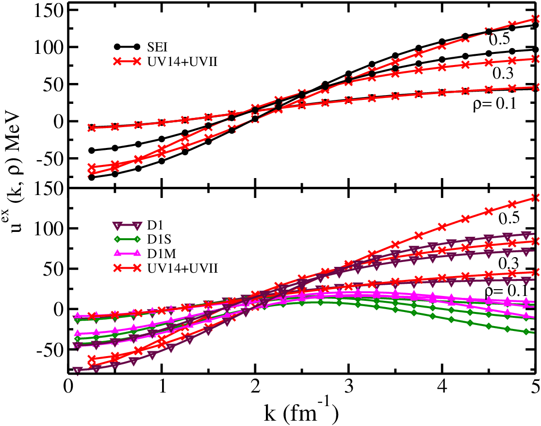
alongwith , and are the six parameters needed for a complete description of the mean field properties and the EOS in SNM. The way of determining the parameters which enter in Eqs. (7) and (8) in this case is similar to the one described in Ref. [58] for a Yukawa form factor. The only difference in this work is that we take the kinetic energy term in its non-relativistic form for convenience of application to finite nuclei. The range parameter and the exchange strength combination in SNM are determined by adopting a simultaneous optimization procedure with the constraint that the attractive optical potential changes sign for a kinetic energy =300 MeV of the incident nucleon (see Ref. [54] for details). In this way the values =-94.46 MeV and =0.7596 are found where we have used only the standard values of the nucleon mass =939 MeV, Fermi kinetic energy =36.4 MeV (the Fermi momentum is with a saturation density =0.157 ) and energy per particle in SNM = -16.0 MeV. The momentum dependence of the nuclear mean field in SNM computed using this SEI for three different densities, =0.1, 0.3, and 0.5 , is displayed in the upper panel of the Fig. 1. In order to compare with the predictions of the realistic interaction UV14+UVII [18], we plot as functions of . Here the saturation properties of the interaction have been substracted because they may be model dependent. We find a quite good agreement between the results computed with the SEI and the microscopic predictions over a wide range of momenta and densities. The same comparison is shown in the lower panel of Fig 1. for Gogny D1 [32], D1S [34] and D1M [36] sets with the microscopic results [18]. We see that the momentum dependence of the Gogny D1 force agrees well with the microscopic results upto density over the whole range of momentum shown in the figure, but agreement of the results become qualitative at higher density as can be seen from the comparison for the curve corresponding to . On the otherhand, the Gogny D1S and D1M forces do not follow the trends of the microscopic calculation beyond ¿ 2 . It may be pointed out that the Gogny forces are fitted basically to finite nuclei data and, therefore, there is no reason a priori for reproducing the momentum dependence of the microscopic calculation in NM over a wide range of momentum in case of all the Gogny force sets.
The effective mass in SNM is given by,
| (10) |
which is momentum and density dependent and can be calculated once the exchange part of the mean field in Eqn. (8) is known. For the values of the exchange strength and range determined above, the prediction of the effective mass at saturation density and momentum is =0.709. The parameter has been adjusted to avoid a supraluminous behaviour at high densities in SNM at =0 (see Ref. [71] for more details). With the standard values mentioned before we obtain =0.5914 . The two remaining strength parameters and are obtained from the saturation conditions. The exponent , that determines the stiffness of the EOS of SNM, is taken as = which gives a value of incompressibility at normal NM density, =245 MeV. With the six parameters of SNM determined, one can calculate the energy per particle and pressure in SNM. These quantities are displayed as a functions of the density in Fig. 2(a) and 2 (b), respectively. They are compared with the values of and predicted by some microscopic calculations and several non-relativistic and relativistic models. In Fig. 2(b) we also display the band of allowed values of in the range extracted from the analysis of the flow data in high energy HIC experiments [72]. Further experimental information of the pressure-density relationship is provided by the analysis of production data [73] in the low density domain between . We find that our SEI curve , obtained using a value of =1/2 passes well within these experimentally extracted regions.
The complete study of ANM now requires the splitting of the three strength parameters , and into two specific channels for interactions between like and unlike pairs of nucleons. We have fixed the splitting of into the like channel to be . This is the critical value for which the thermal evolution of NM properties in pure neutron matter (PNM) does not surpass the SNM results at any density for any temperature [60]. The splitting of the exchange strength parameter into and channels fully determines the - effective mass behaviour in ANM. The - effective masses in ANM are calculated starting from their usual definitions,
| (11) |
The magnitude of the splitting of the n,p-effective masses in ANM at normal density, , obtained with the SEI is shown in Fig. 3 as a function of the asymmetry alongwith the results of microscopic calculations and the values obtained with the Gogny effective forces. Our result compares well with the prediction of the DBHF calculations using the Bonn potential [3] over the whole range of asymmetry . The Gogny D1 interaction also predict closely the similar trend as that of our SEI. But, the effective mass splittings obtained using the Gogny D1S and D1M interactions are very similar between them and have a smaller value as compared with DBHF result. On the other hand, the splittings in the cases of BHF+3-BF and EBHF+3-BF [8, 9, 74] calculations are found to be close to each other, predicting a larger effective mass splitting than the DBHF model.
Once the like and unlike components of are fixed, the splitting of the two remaining strength parameters combinations, namely and can be obtained from values of symmetry energy and its derivatives computed at saturation density. We have assumed a value of =35.0 MeV which is within the possible range between 30-35 MeV [75, 76, 77, 78, 31]. The value of is ascertained from an universal high density behaviour of the asymmetric contribution of the nucleonic part of the energy density in charge neutral beta-stable matter [58, 28]. The value =25.42 MeV obtained in this way predicts a slope parameter (symmetry pressure) =76.3 MeV that is well within the range MeV of recent Finite Range Droplet Model (FRDM) prediction [79]. Our value also lie within the window 45-80 MeV estimated from a compilation of different predictions of deduced from experiments involving antiprotonic atoms, heavy-ion reactions, proton scattering, nuclear masses, microscopic calculations and giant dipole resonances [80]. The values of the nine parameters altogether necessary for a complete description of SNM and ANM alongwith the NM properties (saturation density , binding energy per nucleon in SNM , incompressibility , symmetry energy and slope parameter ) are given in Table I. The strength parameters in SNM can be obtained from this table using the relations of Eqn. (9).
Once the nine parameters that fully determine the ANM are known, the energy per particle in PNM, , can be easily calculated and their values as a function of the density are displayed in Fig. 4 alongwith the results of realistic [81] and some effective models. In the low density region, , it has been verified that our curve passes well through the region predicted by different microscopic calculations performed using Quantum Monte Carlo techniques [82] as it can be seen in the inset of this figure. In the high density region the SEI curve shows a stiff behaviour because of the relatively high value of . The effective M3Y-P5 [38] curve has a relatively more soft behaviour throughout the density range but maintains an increasing trend unlike the case with the D1S Gogny force displayed in the same figure. Further, the EOS of PNM predicts a ratio =1.0 MeV , which is in agreement with the value obtained by Piekarewicz [83] from an analysis of the relation between the slope parameter and the pressure of PNM at normal density . The density dependence of nuclear symmetry energy, , calculated as the difference between the energy per particle in PNM and SNM, is displayed in Fig. 5. It compares well with the results provided by the realistic A18+v+UIX* interaction [17] upto a density 0.2 and follows a similar trend till a density 0.8 . Our curve also compares reasonably well with the DBHF [8, 9] results upto a density of 0.5 , but clearly differs beyond this point where this microscopic calculation shows a very stiff behaviour of the symmetry energy with increasing density.
III nuclear matter under isospin, spin and spin-isospin asymmetries
In the previous section we have restricted our NM study to the case of isospin asymmetric NM, i.e., ANM, which has much physical relevance from the point of view of the available experimental and empirical constraints. However, in order to examine the predictions of SEI in the spin and spin-isospin channels, we shall make first the explicit formulation of NM having both spin and isospin asymmetries. The total NM density is now given by
| (12) |
where, , (, ) denote the neutron spin-up and spin-down (proton spin-up and spin-down) states and , , and are the respective densities. The Fermi-momenta corresponding to these four densities are expressed as
| (13) |
with =n,p and =u,d. Making Taylor expansion of the energy density around the spin-saturated SNM value and keeping terms upto lowest order only, one can obtain
| (14) |
where , and are the , and asymmetries defined as
| (15) |
and , and are the respective symmetry energies. The expressions of these symmetry energies are given by,
| (16) |
where, are the spherical Bessel function of order , , being the Fermi-momentum in saturated SNM, and is the range of the interaction. In these equations , , and are the interactions in the , , and states respectively. Calculation of the symmetry energies using Eqn. (16) requires to know the interactions in all these four different states independently. In the case of the SEI, this is possible provided that all the eleven parameters of the interaction are known. The study of ANM performed in the previous section allows to fix nine of them. The two open parameters ( and considered here) are determined from the study of finite nuclei as will be explained in the next Section. To complet the study of NM matter in the spin and spin-isospin channels we will use the numerical value of the parameters of the SEI interaction reported in Table II.
We first calculate the contributions of the (SO), (SE), (TO) and (TE) states to the potential energy per nucleon in saturated SNM. These contributions, computed using the SEI, are displayed in the four panels of Fig.6 as functions of the Fermi-momentum along with the results for the Gogny D1S and M3Y-P5 interactions. The odd-states contributions of SEI and D1S have a similar behaviour, being attractive in the SO and repulsive in the TO channels. However, these contributions computed with the M3Y-P5 force show a rather strong repulsive character in both odd channels. In the TE channel the contributions computed with the three interactions have a similar behaviour, being attractive upto 2 and thereafter they become strongly repulsive. In the SE channel, the contributions computed with the three forces show the same behaviour upto a Fermi-momentum corresponding to normal NM density. Thereafter the attraction decreases and becomes repulsive at relatively small value in case of SEI and at a larger value for M3Y-P5. On the contrary, the attractive contribution of D1S in the SE channel increases when the Fermi momentum increases.
The density dependence of , and symmetry energies computed with Eqns. (16) using the SEI are displayed in the three panels of Fig.7. The corresponding results obtained with the Gogny D1S [34], D1N [35] and D1M [36] forces are also shown in the respective panels. The symmetry energy , in case of the SEI, has a strong repulsive density dependence in comparison with the considered Gogny forces and does not predict a preferred PNM than SNM at any density. In the case of the symmetry energy , however, the Gogny forces show a very strong density dependence as compared to the behaviour exhibit by the SEI. This is mainly due to the = 1 value in the Gogny forces, which makes the contribution of the density dependent term of the spin symmetry energy highly repulsive. In the spin channel although the SEI has a relatively soft behaviour, as the D1M Gogny force in isospin channel, it does not exhibit instability related to the transition of unpolarized to polarized PNM. A value of =26.55 MeV is obtained in comparison to 27.57 MeV (D1), 29.13 MeV (D1S), 22.69 MeV (D1N), 28.73 MeV (D1M) and 41.01 MeV (M3Y-P5). The symmetry energy shows a similar trend either computed with the SEI or with the Gogny forces, except D1. It reaches a maximum value and decreases becoming zero at certain densities and thereafter remains negative. However, the Gogny D1 interaction shows extra stability in the channel. The density at which the curve of SEI crosses the -axis is larger than the crossing density in the case of the three curves corresponding to Gogny D1S, D1N and D1M. A value of =23.09 MeV is obtained as compared to 30.13 MeV (D1), 29.13 MeV (D1S), 22.69 MeV (D1N), 28.73 MeV (D1M) and 41.01 MeV (M3Y-P5). In Fig. 7(a), the symmetry energy, calculated as the difference of the energy per particle in PNM and SNM, is also shown for comparison with the corresponding results of obtained from the Taylor series expansion of the energy density in Eqn.(16). In NM- calculations, the former definition of the symmetric energy is widely used. It is exact at the two extremes of asymmetry. The comparison between the two, and , is excellent over the whole range of density. The small difference is attributed to the higher order contributions of the Taylor series expansion which have been neglected.


| 0.5914 | 0.7596 | -94.76 | -125.95 | 77.507 | 97.247 | -78.78 | -111.69 | |
| Nuclear matter properties at saturation condition | ||||||||
| () | (MeV) | (MeV) | (MeV) | (MeV) | ||||
| 0.157 | -16.0 | 245 | 0.709 | 35.0 | 76.26 | |||


IV Finite Nuclei
As we mentioned at the Introduction, our aim in this Section is to explore the ability of the SEI in describing ground-state properties of finite nuclei. In Section II we have shown that information of NM allows to determine nine of the eleven parameters of the SEI. Keeping these nine parameters fixed, we will determine the two remaining open parameters, namely and , as well as the strength of the spin-orbit interaction, , from experimental data of some magic nuclei. Once the SEI is fully determined, we will perform some additional calculations to check the predictions of our model in other finite nuclei. We will restrict this preliminary study to spherical nuclei only and leave for a future work the investigation of the deformation properties of the SEI. For open shell nuclei we have to add pairing correlations. As we will explain below with some detail, we use the BCS approach together with a zero-range density-dependent pairing interaction that was devised to simulate the behaviour of the Gogny D1 pairing gap in neutron matter [84].
IV.1 The quasilocal Density Functional Theory
To deal with finite nuclei, we apply the KS [64] method within the framework of the non-local DFT [68]. As it is proved in this reference, the Lieb theorem [85], which establish the many-to-one mapping of a -particle Slater determinant wavefunctions onto the local particle density , allows to write the energy density functional in the non-local case as . Here is the Slater determinant DM with occupation numbers either 1 or 0 and has the form of the HF energy obtained with an effective Hamiltonian . The remaining part, , that is a functional of the local density only, is the residual correlation energy. This contribution accounts for the difference between the exact energy functional, constructed with the true microscopic Hamiltonian , and the HF energy provided by the reference Hamiltonian . In Ref. [68] it is also shown that another reduction can be performed by mapping the Slater DM onto a set of local particle, kinetic energy and spin densities for neutron and proton, i.e. . The particle, kinetic energy and spin local densities entering in the set are obtained from the single-particle orbitals that define the Slater determinant as
| (17) |
| (18) |
and
| (19) |
respectively.
Using this reduction, it is possible to write finally the energy density functional in a quasilocal form as . By applying the variational principle to the functional and using as functional variables the single-particle orbitals and , one obtains the corresponding KS equations. We shall point out that within this quasilocal theory, one would be able to compute the exact ground-state energy and the exact local particle densities if the exact density functional is known. However, the kinetic energy densities, and , as well as the spin densities, and , correspond to uncorrelated system and therefore do not concide with the exact densities within this approach. As explained in [68], there is some freedom in the choice of the effective Hamiltonian . Therefore, we can choose as an -particle effective interaction of the type . The nucleon-nucleon interaction contains the contriutions of the effective force that we take in this work as the density-independent finite-range part of the SEI in Eqn. (1), and the spin-orbit contribution chosen in the form used in the Skyrme and Gogny interactions: . From this effective Hamiltonian we obtain the quasilocal energy functional as:
| (20) |
where the energy density reads
| (21) | |||||
The kinetic energy part corresponds to the non-interacting contribution given by Eqn. (18). The Coulomb energy is taken in the usual way as the direct term plus the exchange contribution computed at Slater level using the point proton density:
| (22) |
The spin-orbit energy density, computed using the aforementioned zero-range force, becomes:
| (23) |
The direct contribution to the nuclear energy coming from finite range part of the SEI is given by
| (24) |
All these local contributions to the energy density constitute the so-called Hartree part of the functional. Up to this point, we have developed the exact theory. In the next step we shall make some approximations, similar to those used in Refs. [1, 62, 63]. To compute the quasilocal energy density corresponding to the exchange terms of the nucleon-nucleon force, SEI in this case, we use the Extended Thomas-Fermi (ETF) expansion of the DM up to order which is widely discussed in Ref. [69]. For spin-saturated nuclei the exchange nuclear energy density splits into two part
| (25) |
The first term corresponds to the zeroth order of the -expansion (Slater approximation for the density matrix) given by
| (26) |
where, and are the relative and center of mass co-ordinates, respectively. In Eq.(26) and is the spherical Bessel function. The second term of Eqn.(25) is the contribution to the exchange energy which reads [69, 68]
| (27) |
Here and . The function is the inverse of the position and momentum dependent effective mass given by
| (28) |
In this equation is the Wigner transform of the exchange potential,
| (29) |
where and . Notice that in the ANM limit is just the exchange part of the mean field in Eqn. (6) and therefore, in this limit, the inverse effective mass reduces to Eqn. (11).
It is worth noting that within the semiclassical ETF expansion of the DM the kinetic energy is a functional of the local density only. However, it was found in [69] that the use of the quantal kinetic energy density (18) in the -contribution to the exchange energy (27), significantly improves the agreement with the corrersponding full HF calculation. Therefore, we will use this ansatz here as it was done in previous works [69, 68, 89]. It is also important to note that we have repalced the exact quasilocal functional by an approximated one calculated with the ETF prescription. The difference between them gives a very small contribution that cannot be completely included in the residual correlation energy because the difference depends on (through , , and ) while depends on only. Notice, however, that this small difference, due to the localization of the exchange energy, persists if one uses another DM expansions as the Negele-Vautherin [62] or Campi-Bouyssy [63] ones.
Let us now discuss the residual correlation energy part of the total energy density. The SEI, as it happens with another finite-range forces as the Gogny or M3Y ones, can be split into a density-independent and a density-dependent parts. Therefore, a reasonable ansatz, in the spirit of the DFT, is to take the residual correlation energy as the HF contribution provided by the density-dependent part of the interaction in ANM in a local density approximation:
| (30) | |||||
As mentioned before, the variational principle applied to the full functional allows to obtain the following set of KS single particle equations:
| (31) |
where,
| (32) |
and
| (33) |
that are formally similar to the equations of motion obtained with zero-range Skyrme forces. The quasilocal DFT presented in this work is, actually, very similar to the one used by Hoffman and Lenske in Ref. [2]. The main difference is that the localization of the exchange energy is performed here using the ETF expansion of the DM while in Ref. [2] the Campi-Bouyssy expansion of the DM is used. As it is pointed out in this reference [2], the DM expansions retain, to certain extension, the non-local effects of the underlying interaction. In the case of the ETF expansion of the DM these effects are collected in the effective mass and its derivative respect to the momentum which appear in Eqn. 27.
In Ref. [68] we have chosen the parameters of in and the ones of to be equal to the parameters of the Gogny D1S force. In this way we check to which extend the quasilocal KS-DFT approach is able to reproduce the full HF results with this interaction. We have performed the same comparison with the D1N and D1M forces. It is found that the difference between the HF and the quasilocal KS-DFT energy per nucleon in magic nuclei is always smaller than 0.01 MeV in 48Ca, 90Zr and 208Pb for all the Gogny forces considered. For light nuclei the differences in the binding energy per nucleon are a little bit larger but smaller than 0.09 MeV per nucleon in 16O and than 0.05 MeV per nucleon in 40Ca for these Gogny forces (See also Table I of [69]). These results show that the quasilocal energy density functional obtained with the KS-DFT formalism explained here describes ground-state properties of finite nuclei fairly well. This fact motivates us to use directly the quasilocal energy density functional obtained with the SEI fitting its undetermined parameters, and of the and the strength of the spin-orbit interaction , to experiemntal data.
| W | B | H | M | ||||||||
| 0.5914 | 437.0 | 0.6 | 9955.2 | -0.118 | -589.09 | 130.36 | -272.42 | -192.16 | 0.7596 | 115.0 |
| Nucleus | Force | BE/A | |||
|---|---|---|---|---|---|
| 16O | SEI | 7.976 | 2.764 | 2.622 | 2.646 |
| Gogny (D1S) | 8.099 | 2.783 | 2.645 | 2.666 | |
| M3Y-P5 | 7.88 | ||||
| RMF (NL3∗) | 8.007 | 2.735 | 2.465 | 2.615 | |
| Expt. | 7.976 | 2.730 | |||
| 40Ca | SEI | 8.551 | 3.484 | 3.346 | 3.391 |
| Gogny (D1S) | 8.616 | 3.501 | 3.365 | 3.408 | |
| M3Y-P5 | 8.38 | ||||
| RMF (NL3∗) | 8.539 | 3.470 | 3.237 | 3.377 | |
| Expt. | 8.551 | 3.485 | |||
| 48Ca | SEI | 8.680 | 3.510 | 3.597 | 3.418 |
| Gogny (D1S) | 8.681 | 3.534 | 3.583 | 3.442 | |
| M3Y-P5 | 8.63 | ||||
| RMF (NL3∗) | 8.617 | 3.470 | 3.517 | 3.377 | |
| Expt. | 8.666 | 3.484 | |||
| 90Zr | SEI | 8.708 | 4.275 | 4.285 | 4.199 |
| Gogny (D1S) | 8.729 | 4.285 | 4.267 | 4.210 | |
| M3Y-P5 | 8.66 | ||||
| RMF (NL3∗) | 8.693 | 4.263 | 4.227 | 4.187 | |
| Expt. | 8.710 | 4.272 | |||
| 208Pb | SEI | 7.867 | 5.498 | 5.643 | 5.437 |
| Gogny (D1S) | 7.879 | 5.494 | 5.569 | 5.435 | |
| M3Y-P5 | 7.85 | ||||
| RMF (NL3) | 7.876 | 5.508 | 5.680 | 5.450 | |
| Expt. | 7.867 | 5.505 |

| Z or N | |||
|---|---|---|---|
| Chain | SEI | Ref. [111] | Ref. [112] |
| Z= 20 | 0.85/0.62 | 0.82/0.76 | 1.02/0.92 |
| Z= 50 | 0.55/0.62 | 0.29/0.21 | 0.43/0.35 |
| Z= 82 | 0.46/0.82 | 0.23/0.37 | 0.58/0.53 |
| N= 50 | 0.22/0.24 | 0.37/0.26 | 0.41/0.23 |
| N= 82 | 0.21/0.42 | 0.43/0.31 | 0.50/0.56 |
| N= 126 | 0.67/0.51 | 0.42/0.23 | 0.88/0.52 |
| Z or N | ||||
|---|---|---|---|---|
| Chain | NL3 [108] | SLy4 [115] | SkM* [115] | D1S [116] |
| Z= 20 | 0.99 | 0.58 | 1.90 | 0.94 |
| Z= 50 | 0.99 | 0.89 | 1.48 | 0.90 |
| Z= 82 | 1.09 | 1.24 | 1.25 | 0.98 |
| N= 50 | 1.05 | 0.53 | 1.03 | 0.93 |
| N= 82 | 1.03 | 0.29 | 1.87 | 0.47 |
| N= 126 | 1.56 | 0.72 | 2.16 | 0.91 |


Certainly, pairing correlations play an important role for open shell nuclei. To deal with such nuclei, it is mandatory to include the pairing correlations. The first formal generalization of the Hohenberg-Kohn theorem to paired systems was performed in Ref. [86] for superconductors. Some modifications of this approach were developed later in Refs. [87, 88]. More recently, in Ref. [89], an extension of the DFT including pairing correlations without formal violation of the particle-number conservation and the quasilocal reduction of this non-local theory are discussed with detail. The equations of motion associated to this energy density functional including pairing correlations have the same form as the HFB equations. However, for pairing calculations of nuclei not too far from the -stability line, the simpler BCS approach can be sufficient for describing their ground-state energies [90]. For these nuclei, the Fermi level lies appreciably below zero and, consequently, the levels around it, which mainly contribute to pairing correlations, are also well bound avoiding the problems of the standard BCS approach near the drip lines [91, 92]. For practical BCS calculations, one extracts from the energy density functional a part which depends only on the normal density and that describes the nuclei without pairing effects. The remaining part contains the contributions arising from the pairing correlations. In the BCS approach the motion equations, in the case of spherical symmetry, reduces to a set of mean-field single-particle equations, that in the quasilocal approach are given by Eq. (31), and another set of gap equations
| (34) |
In the gap equations (Eqn. (34)), are the quasiparticle energies with the single-particle energies, the state dependent gaps and the chemical potential to ensure the right number of particles. In this equation are the reduced matrix elements of the effective interaction in the particle-particle channel. Eqns. (31) and (34) are coupled among them and have to be solved self-consistenly. In Refs. [89, 93] the ability of this quasilocal extension of the DFT including pairing correlations at BCS level to reproduce full HFB binding energies and gaps was checked. The calculations were performed for several Sn and Pb isotopes lying in the stability valley using the Gogny D1 and D1S forces in both, particle-hole and particle-particle, channels. In these test calculations the differences between the full HFB and the quasilocal approach plus BCS are less than 0.2%, which are similar to the values found for magic nuclei [68].
In this paper we will use this formalism for the study of the binding energies of some open shell spherical nuclei. To this end we will use the mean field provided by the SEI. For a sake of simplicity we chose as pairing interaction a density-dependent zero-range force of the type proposed by Bertsch and Esbensen [94]:
| (35) |
This effective pairing force is extensively used in nuclear structure calculations [95, 96, 89, 19, 97, 98, 99]. The numerical values of the parameters =-481 MeV , =0.45, =0.47 and =0.16 are taken from Ref. [84]. These parameters, together with a cutoff energy =60 MeV from the bottom of the single-particle potential, were fitted in [84] to reproduce the gap values of the Gogny D1 force in neutron matter. We use here an improved BCS approach [23] where the resonant levels [92] are simulated very efficiently by quasibound single-particle energy levels retained by the centrifugal (neutrons) or centrifugal plus Coulomb (protons) barriers. The two-body center of mass correction has been taken into account self consistently by using a pocket formula based on the harmonic oscillator and derived in Ref. [100].
IV.2 Results of finite nuclei
In order to determine the three parameters, , and , we proceed as follows. Keeping the nine parameters determined in ANM (see Table I) fixed, (i) We reproduce the experimental binding energy of 40Ca by adjusting , (ii) The spin-orbit strength parameter is adjusted to reproduce the experimental splitting of the neutron and proton levels in 16O (iii) The parameter is obtained by fitting the binding energy and charge radius of 208Pb. The steps (i)-(iii) are repeated till the self-consistency of the parameters , and is achieved. The value of the eleven parameters of the SEI entering in Eqn. (1) as well as the strength of the spin-orbit force are given in Table II.
The binding energy per particle (BE/A) and the proton (), neutron () and charge ( ) rms radii of the standard magic nuclei computed with the SEI quasilocal energy density functional are displayed in Table III. These results are compared with the corresponding values obtained using the Gogny (D1S) [33, 34] and the M3Y-P5 [38] forces and the RMF (NL3∗) parametrization [25] as well as with the experimental data (binding energies from [101] and charge radii from [102]) that are also displayed in Table III. It is observed that the BE/A obtained with the SEI functional matches nicely with the experimental data for these magic nuclei . In case of radii, our results are similar to those provided by the Gogny and the RMF calculations. The neutron skin thickness, defined as the difference between the neutron and proton rms, i.e. , in 208Pb predicted by our calculation using the SEI functional is 0.21 . This value is in agreement with the experimental result obtained in Ref. [103] using proton-nucleus scattering.
Experimental information about single-particle energies of even-even nuclei can be obtained from the low-lying excited states of the adjacent odd nuclei by adding or picking up a single nucleon. The ordering of the particle and hole levels, for both neutrons and protons, predicted by the SEI functional is in agreement with the experiment [104, 105] except for the neutron level which lies below the one. This is, however, a relatively common fact in many mean field models, as for example the well reputed NL3 [106]. The level spacing predicted by the SEI functional is larger than the experimental one, but similar to the spacing obtained with the D1S and M3Y-P5 forces. The spin-orbit splittings of the single-particle levels and of neutrons and of protons obtained with our functional overestimate the experimental values as it also happens with the D1S and M3Y-P5 predictions.
The radial dependence of the density distributions for protons and neutrons of the nuclei 16O, 40Ca, 48Ca and 208Pb are displayed in the four panels of Fig. 9. The neutron and proton densities for the same nuclei obtained using the RMF (NL3) [24] alongwith the experimental data for charge distributions, taken from Ref. [107], are also given for comparison in the same figure. For 16O, 40Ca and 48Ca the agreement between our densities and the ones predicted by NL3 model is quite good. The density distributions of 208Pb computed with SEI and NL3 differ more between them, mainly in the bulk region. The proton densities predicted by the SEI functional agree reasonably well with the experimental charge distributions at the surface. In the interior of the nucleus the quantal oscillations shown by our proton densities are, in general, well averaged.
From Table III it is seen that the SEI functional predicts ground-state energies and radii that accurately reproduce the experimental values. In this respect, the following comments are in order. To determine the nine parameters of ANM, we have considered the empirical values of three NM parameters, namely , and . The widely accepted ranges of these parameters are =0.170.03 , =-160.02 MeV and =30-35 MeV. We have examined the variations of these parameters within their ranges and have found that small variations in the values of , and have a large influence on the predictions of binding energies and radii in finite nuclei, although the changes in the NM predictions are not of much significance. It is also found that critically depends on the value of that determines the stiffness of EOS in SNM. For a given value of , there is a critical value of for which the predictions of binding energies and radii will have minimal deviation from experimental results. Thus for the EOS considered in this work corresponding to =1/2, the best results in finite nuclei are found for =0.157 , = -16 MeV and =35 MeV.
We have performed further investigations to check the ability of our proposed SEI functional to describe ground-state properties of spherical nuclei. In this exploratory calculation pairing correlations are treated at BCS by the reasons pointed out before. Notice, however, that the BCS approach for pairing has been used in several well known mass tables as the ones computed with NL3 [108] and HFBCS-1 [109]. In the upper panel of Fig. 10 we display the two-neutron and the one-neutron separation energies for Sn isotopes and in the lower panel of the same figure the two-proton and one-proton separation energies for the N=82 isotonic chain. To obtain the one-neutron and one-proton separation energies we have to compute odd-even or even odd-nuclei. To deal with these nuclei we perform, as in Ref. [38], spherical blocking calculations which neglect part of the core polaritazion effect in the odd nuclei [90]. In these calculations one has to block several single-particle states around the Fermi energy and search for the configuration giving the lowest energy. From Fig. 10, we see that the SEI predictions match fairly well with the experimental values for both chains. To be more quantitative, we have also computed the two- and one-nucleon separation energies in other isotopic and isotonic chains with magic proton and neutron numbers, respectively. In Table IV we show the rms deviation of these separation energies with respect to the experimental values [101] for the =20, 50, 82 isotopic and =50, 82, 126 isotonic chains. Our predictions are compared with the HFB results of Refs. [111] and [112] (see the former reference for more details). A similar comparison between our results and the ones provided by the SLy4 and Gogny D1S forces and the NL3 parameter set, but only for two-nucleon separation energies is given in Table V. From Table IV, it can be seen that our results are not so good than those of [111] but similar to the ones of [112]. Notice, however, that in Refs. [111] and [112] the strength of the pairing force is fitted to some experimental data while in our case the pairing interaction is taken from the literature without any refit of their parameters to experimental data. The quality of the our predictions for two-nucleon separation energies also compare very satisfactorily with the results obtained from HFB calculations with SLy4 and SkM∗ [115] and D1S [116] forces and the ones calculated with the NL3 parameter set [108].
We have performed more tests to check the ability of the SEI energy density for describing ground-state properties of finite nuclei. To this end, we have computed the binding energy and charge radii of 161 even-even spherical nuclei between 16Ne and 224U. The difference between the theoretical prediction and the experimental value for binding energy and charge radius are shown in the upper and lower panel of Fig. 11, respectively. In general, the deviations in binding energies and charge radii for the -spherical nuclei are broadly reproduced within MeV and , respectively, baring few exceptions. The overall rms deviation in energy and charge radius of these nuclei are =1.5402 MeV and = 0.0152 , respectively. These values are a little bit smaller than the corresponding rms deviations obtained with well calibrated effective interactions as D1S, SLy4, NL3 and BCP for the same set of nuclei (see Table 3 of Ref. [19]). We have also estimated 303 binding energies and 111 charge radii of odd spherical nuclei, for which the experimental values are known. For these nuclei we find =1.6501 MeV and = 0.0198 , respectively.
Using our SEI, we have also computed the isotopic shift of charge radii, defined as , in Pb-isotopes. Analyzing the values obtained with the SEI, one can see in Fig. 12 that they lie quite close to the experimental values [102] and that the kink at =208 is reasonably well reproduced. It is known that Skyrme and Gogny forces use isospin independent spin-orbit interactions those are unable to reproduce the experimental kink exhibit by the isotopic shift of the charge radius in Pb isotopes at the double magic 208Pb [114, 113]. This mismatch can be cured by introducing an isovector spin-orbit contribution as it is the case of the SkI family of Skyrme forces [114] or using non-linear RMF parametrizations [117]. However, the SEI functional incorporates a spin-orbit contribution that does not contain isovector part (see Eqn.(23)) but clearly shows up the kink without imposing it as a constraint in the fitting procedure of the functional. A possible explantion is the following. In a recent paper [118] it is claimed that the development of the kink in the isotopic shift of the charge radius of 208Pb is largely determined by the occupation of the neutron level. This orbital has a principal quantum number =1 and overlaps strongly with the majority of the proton orbitals. This produces a relatively large pulling of the proton orbitals by the neutron ones via the symmetry energy increasing the proton radius, and, therefore, developing the kink at . From Fig.8 we can see that the SEI functional predicts that the lies close to the one and the same happens for heavier Pb isotopes. Therefore, one can expect a relatively large occupation of state. This fact together with the relatively high symmetry energy of the SEI seems to be the reason for the appearence of the kink exhibit by the SEI results in Fig.12.
We shall now discuss in some detail the pairing properties of our SEI energy density functional. This functional includes a pairing contribution coming from a zero-range density-dependent force that simulates the Gogny interaction in the particle-particle channel. As far as the Gogny pairing force gives a good description of finite nuclei combined with a reasonable mean field, not only provided by the Gogny interaction but also by Skyrme forces and RMF parametrizations [25], we are, actually, checking the single-particle energies obtained with the SEI energy density functional. In Fig. 13 we display the average gaps along the whole Sn isotopic chain obtained with our formalism compared with the values predicted by a full HFB calculation with the Gogny D1S force in both, particle-hole and particle-particle, channels. From this figure it can be seen that the averaged gaps, defined as and nicely reproduce the HFB values in this isotopic chain taken of Ref. [92]. This result suggests that our model, with a mean field part whose parameters are fitted to ANM and magic nuclei together with a realistic pairing force taken from the literature, is, in principle, well suited for describing open-shell nuclei at mean field level with a quality similar to that found using well known effective interactions or RMF paramtrizations.
A possible way of estimating pairing correlations from an experimental point of view is through the so-called odd-even mass staggering (see e.g. Ref. [90]). In Fig. 14 we display the odd-even mass staggering using a three-point formula [90]
| (36) |
for the Sn isotopic chain (upper panel) and for the =82 isotonic chain computed with the SEI energy functional in comparison with the experimental values. Our theoretical prediction of the mass staggering slightly overestimate the experiemental values in both, Sn isotopic chaim and =82 isotonic chain. Therefore, some comments are in order. On the one hand, the odd-even mass staggering of experimental masses is not a pure measure of the pairing correlations [90]. It also contains mean field contributions related to the rotational and time-reversal symmetries breaking not accounted by the simple blocking approach. On the other hand, the fact that the theoretical odd-even mass staggering overestimates the corresponding experimental values may be not so dramatic. It is known that when pairing is computed using the Gogny interaction, the average gaps are larger than the mass gap [32]. However, as discussed in this reference, effects beyond mean-field, such as quasiparticle vibration coupling, are expected to reduce the average gaps. Finally to point out that in this exploratory calculation no attempt has been done in order to adjust simultaneously pairing and mean field. Therefore, it seems reasonably that a slightly different protocol in the fitting procedure of the parameters and , for example including some open shell in it, would allow to find an odd-even mass staggering in better agreement with the experimental data. From all the discussion developed along this section, we believe that the reported calculations show up clearly that the proposed energy density functional based on the SEI is a realiable tool for dealing, at least in spherical nuclei, with quality similar to that found using well calibrated Gogny or Skyrme forces or succesful RMF paraametrizations in the same scenario.
V Summary and conclusions
We have proposed a simple effective interaction aimed to describe accurately the main trends of microscopic calculations in nuclear and neutron matter and, at the same time, to reproduce the ground state properties of finite nuclei with a quality similar to the one obtained using successful effective interactions of Skyrme, Gogny and M3Y type or relativistic mean field model. Our interaction contains a single Gaussian form factor for describing the finite range part of the force plus a zero-range part that includes a density dependent term to simulate the effect due to three-body forces. Our effective interaction depends on eleven parameters, nine of them fitted to nuclear and neutron matter data. The SNM is fully determined by six parameters, which are three strength combinations, the range of the force, the exponent and the factor . Two of these six parameters, the strength of the exchange interaction and the range of the force, completely determine the momentum dependence of the mean field in SNM. These two parameters are constrained by using the optical potential data which imposes that the calculated mean field in normal SNM vanishes at a kinetic energy MeV of the incident nucleon. The exponent of the density dependent term is chosen amongst the values that gives the pressure-density relation in agreement with the experimental results of HIC and production. The parameter is fixed to avoid the supraluminous behaviour in NM. The two remaining strength combinations in SNM are determined from the saturation conditions. In our model, the range of the force is chosen to be the same for interactions between pairs of like and unlike nucleons. Under this restriction, the splitting of the exchange strength parameter in ANM is decided from the condition that the entropy in PNM does not exceed the one in SNM. The splitting of the two other strengths into like and unlike channels in ANM are decided from the value of the symmetry energy and by imposing that the nucleonic part of the energy density in charge neutral -stable matter be a maximum. With the nine parameters of our effective interaction determined in this way, the corresponding EOS and mean field follow, quite closely, the general trends shown up by sophisticated microscopic calculations.
To describe finite nuclei we use this interaction to build up an energy density functional in the framework of the quasilocal Density Functional Theory. In particular we use the semiclassical - expansion of the density matrix to deal with the exchange contribution. This procedure allows to write the single particle equations in finite nuclei in a similar form as in the case of the Skyrme-Hartree-Fock equations. We determine the open parameters of our interaction and , and the strength of the spin-obit force by a simple fit to experimental data of three closed shell nuclei 16O, 40Ca and 208Pb. With this choice the binding energies and charge radii of the standard magic nuclei are accurately reproduced. With our simplified interaction fully determined, we explore its predictive power for describing open-shell spherical nuclei. To this end, we add to our functional the contribution of a zero-range pairing interaction, taken from the literature, which reproduces the Gogny neutron gaps in PNM. In this exploratory calculation we use the BCS approximation instead of HFB theory for dealing with open shell nuclei and the simplified spherical blocking approach to estimate the ground-state properties of odd nuclei. It is important to note that within this framework, the results for open-shell nuclei are predictions of our model as far as no parameter has been fitted to open-shell nuclei. We have computed the energy of and charge radii of spherical even-even nuclei in the mass region 16-224. Our calculation reproduce the experimental values fairly well. The rms deviations of the binding energies i and radii of these nuclei with respect to the experimental values are MeV and , respectively, which are slightly better than the same results for the set of nuclei computed using standard interactions such as Gogny D1S, BCP, NL3 and SLy4. We have also calculated the one- and two-nucleon separation energies along the Ca, Sn and Pb isotopic chains and =50, 82 and 126 isotonic chains. With our model, the rms deviation of the theoretical predictions respect to the experimental data compares favourably with the results obtained using well calibrated effective interactions of Skyrme, Gogny and relativistic mean field type. We have also investigated the isotopic shift of the charge-radii in Pb. We find, surprisingly, that the kink shown by the experimental charge radii at =208, is qualitatively reproduced by our model, in spite that our spin-orbit force has no isospin dependence, which is needed, in principle, to reproduce the kink with non-relativistic mean field models. We have given a possible explanation of this fact based on the small gap between the and neutron levels and the relatively large symmetry energy predicted by the SEI model.
In this exploratory analysis of finite nuclei properties described with our simplified effective interaction we have restricted to spherical nuclei. To improve the treatment of pairing correlations by replacing the BCS approach by a Hartree-Fock-Bogoliubov calculation, and extend our study to deformed nuclei and some collective excited states is a necessary task to confirm the success of our simplified effective interaction that will be developed in future works.
Acknowledgments
The authors are indebted to P. Schuck and L.M. Robledo by useful disucssions. This work is supported in part by the UGC-DAE Consortium for Scientific Research, Kolkata Center, Kolkata, India (Project No. UGC-DAE CRS/KC/CRS/2009/NP06/1354) and the work is covered under SAP program of School of Physics, Sambalpur University, India. One author (TRR) thanks Department d’Estructura i Constitutuents de Materia, University de Barcelona, Spain for hospitality during the visit. B.K.S and X.V. acknowledges the support of the Consolider Ingenio 2010 Programme CPAN CSD2007-00042, Grant No. FIS2011-24154 from MICINN and FEDER, and Grant No. 2009SGR-1289 from Generalitat de Catalunya. B.K.S also acknowledge the support Grant No. CPAN10-PD13 from CPAN (Spain). One of the author MB acknowledges the support in part by Council of Scientific Industrial Research (File No.09/153(0070)/2012-EMR-I).
References
- [1] F. Hoffmann, C. M. Keil and H. Lenske, Phys. Rev. C 64, 034314 (2001).
- [2] F. Hoffmann and H. Lenske, Phys. Rev. C 57, 2281 (1998).
- [3] F. Sammarruca, Int. J. Mod. Phys. E, 19 1259 (2010).
- [4] D. Alonso and F. Sammarruca, Phys. Rev. C 67, 054301 (2003).
- [5] M. R. Anastasio, L. S. Celenza, W. S. Pong, and C. M. Shakin, Phys. Rep. 100, 327 (1983).
- [6] C. J. Horowitz and B. D. Serot, Phys. Lett. B 137, 287 (1984); Nucl. Phys. A 464 613 (1987).
- [7] R. Brockmann and R. Machleidt, Phys. Lett. B 149 283 (1984); Phys. Rev. C 42 1965 (1990).
- [8] E. N. E. Van Dalen, C. Fuchs and A. Faessler, Nucl. Phys. A 744, 227 (2004).
- [9] E. N. E. Van Dalen, C. Fuchs and A. Faessler, Phys. Rev. Lett. 95, 022302 (2005).
- [10] K. A. Brueckner, C. A. Levinson, and H. M. Mahmoud, Phys. Rev. 95, 217 (1954).
- [11] H. A. Bethe, Phys. Rev. 103, 1353 (1956).
- [12] J. Goldstone, Proc. R. Soc. London, Ser.A 239, 267 (1957).
- [13] H.A. Bethe, Annu. Rev. Nucl. Sci. 21, 98 (1971).
- [14] I. Bombaci and U. Lombardo, Phys. Rev. C 44, 1892 (1991).
- [15] J. Xu, L. W. Chen, B. A. Li and H. R. Ma, Phys. Rev. C 75, 014607 (2007).
- [16] M. Baldo, C. Maieron, P. Schuck and X. Viñas, Nucl. Phys. A736, 241 (2004).
- [17] A. Akmal, V. R. Pandharipande and D. G. Ravenhall, Phys. Rev C 58, 1804 1998.
- [18] R. B. Wiringa, Phys. Rev. C 38, 2967 (1988); R. B. Wiringa, V. Fiks, A. Fabrocini, Phys. Rev. C 38 1010 (1988).
- [19] M. Baldo, P. Schuck and X. Viñas, Phys. Lett. B 663, 390 (2008).
- [20] J. Boguta, A. R. Bodmer, Nucl. Phys. A 292, 413 (1977).
- [21] B. D. Serot and J. D. Walecka, Adv. Nucl. Phys. 16, 1 (1986).
- [22] Y. K. Gambhir, P. Ring, and A. Thimet, Ann. Phys. (N.Y.) 198, 132 (1990).
- [23] M. Del Estal, M. Centelles, X. Viñas, and S. K. Patra, Phys. ReV. C 63, 024314 (2001).
- [24] G. A. Lalazissis, K. Konig, and P. Ring, Phys. Rev. C 55, 413 (1997).
- [25] G. A. Lalazissis, S. Karatzikos, R. Fossion, D. Pena Arteaga, A. V. Afanasjev and P. Ring, Phys. Lett. B 671, 36 (2009).
- [26] T. Niksic, D. Vretenar, P. Finelli, and P. Ring, Phys. Rev. C 66, 024306 (2002).
- [27] G. A. Lalazissis, T. Niksic, D. Vretenar, and P. Ring, Phys. Rev. C 71, 024312 (2005).
- [28] T. Klahn et al., Phys. Rev. C 74 035802 (2006).
- [29] X. Roca-Maza, X. Viñas, M. Centelles, P. Ring and P. Schuck, Phys. Rev. C 84, 054309 (2011).
- [30] D. Vautherin and D. M. Brink, Phys. Rev. C 05, 626 (1972).
- [31] M. Dutra et al., Phys. Rev. C 85, 035201 (2012).
- [32] J. Decharge and D. Gogny, Phys. Rev. C 21, 1568 (1980).
- [33] J. F. Berger, M, Girod, D. Gogny, Nucl. Phys. A 428, 23c (1984).
- [34] J. P. Blaizot, J. F. Berger, J. Decharge, and M. Girod, Nucl. Phys. A 591, 435 (1995).
- [35] F. Chappert, M. Girod and S. Hilaire, Phys. Lett. B 668, 420 (2008).
- [36] S. Goriely, S. Hilaire and M. Girod, Phys. Rev. Lett. 102, 242501 (2009).
- [37] H. Nakada, Phys. Rev. C 68, 014316 (2003).
- [38] H. Nakada, Phys. Rev. C 78, 054301 (2008).
- [39] S. Kubis, M. Kutschera, Phys. Lett. B 399, 191 (1997).
- [40] V. Greco, F. Matera, M. Colonna, M. Di Toro, G. Fabbri, Phys. Rev. C 63, 035202 (2001).
- [41] V. Greco, M. Colonna, M. Di Toro, G. Fabbri, Phys. Rev. C 63, 045203 (2001).
- [42] V. Greco, V. Baram, M. Colonna, M. Di Toro, G. Gaitanos, H. H. Wolter, Phys. Lett. B 562, 215 (2003).
- [43] E. Chabanat, P. Bonche, P. Hansel, J. Meyer, and R. Schaeffer, Nucl. Phys. A 627,710 (1997).
- [44] E. Chabanat, P. Bonche, P. Hansel, J. Meyer, and R. Schaeffer, Nucl. Phys. A 635, 231 (1998).
- [45] E. Chabanat, P. Bonche, P. Hansel, J. Meyer, and R. Schaeffer, Nucl. Phys. A 634, 441 (1998).
- [46] G. F. Bertsch, S. Das Gupta, Phys. Rep. 160, 189 (1988).
- [47] G. M. Welke, M. Prakash, T. T. S. Kuo, S. Das Gupta, C. Gale, Phys. Rev. C 38, 2101 (1988).
- [48] C. Gale, G. M. Welke, M. Prakash, S. J. Lee, S. Das Gupta, Phys. Rev. C 41, 1545 (1990).
- [49] L.P. Csernai, G. Fai, C. Gale, E. Osnes, Phys. Rev. C 46, 736 (1992).
- [50] Q. Pan, P. Danielewicz, Phys. Rev. Lett. 70, 2062 (1993).
- [51] J. Zhang, S. Das Gupta, C. Gale, Phys. Rev. C 50, 1617 (1994).
- [52] P. Danielewicz, Nucl. Phys. A 673, 375 (2000).
- [53] C. Fuchs, Prog. Part. Nucl. Phys. 56, 1 (2006).
- [54] B. Behera, T. R. Routray and R. K. Satpathy, J. Phys. G: Nucl. Part. Phys. 24, 2073 (1998).
- [55] B. Behera, T. R. Routray, B. Sahoo and R. K. Satpathy, Nucl. Phys. A 699, 770 (2002).
- [56] B. Behera, T. R. Routray and A. Pradhan, Mod. Phys. Lett. A 20, 2639 (2005).
- [57] B. Behera, T. R. Routray, A. Pradhan, S. K. Patra and P. K. Sahu, Nucl. Phys. A 753, 367 (2005).
- [58] B. Behera, T. R. Routray, A. Pradhan, S. K. Patra and P. K. Sahu, Nucl. Phys. A 794, 132 (2007).
- [59] B. Behera, T. R. Routray and S. K. Tripathy, J. Phys. G: Nucl. Part. Phys. 36, 125105 (2009).
- [60] B. Behera, T. R. Routray and S. K. Tripathy, J. Phys. G: Nucl. Part. Phys. 38, 115104 (2011).
- [61] G. Bertsch, J. Borysowicz, H. McManus, and W. G. Love, Nucl.Phys. A 284, 399 (1977).
- [62] J. W. Negele and D. Vautherin, Phys. Rev. C 5, 1472 (1972); Phys. Rev. C 11, 1031 (1975).
- [63] X. Campi and A. Bouyssy, Phys. Lett. B 73, 263 (1978); Nukleonika 24, 1 (1979).
- [64] W. Kohn and L. J. Sham, Phys. Rev. 140, A1133 (1965).
- [65] J. Messud, M. Bender and E. Suraud, Phys. Rev. C 80, 054314 (2009).
- [66] P. Hohenberg and W. Kohn, Phys. Rev. 136, B864 (1964).
- [67] T. L. Gilbert, Phys. Rev. B 12, 2111 (1975).
- [68] V. B. Soubbotin, V. I. Tselyaev and X. Viñas, Phys. Rev. C 67, 014324 (2003).
- [69] V. B. Soubbotin and X. Viñas, Nucl. Phys. A 665, 291 (2000).
- [70] M. Stoitsov, M. Kortelainen, S. K. Bogner, T. Duget, R. J. Furnstahl, B. Gebremariam and N. Schunck, Phys. Rev. C 82, 054307 (2010).
- [71] B. Behera, T. R. Routray and R. K. Satpathy, J. Phys G: Nucl. Part Phys. 23, 445 (1997).
- [72] P. Danielewicz, R. Lacey, and W.G. Lynch, Science 298, 1592 (2002).
- [73] W. G. Lynch, M. B. Tsang, Y. Zhang, P. Danielewicz, M. Famiano, Z. Li, and A. W. Steiner, Prog. Part. Nucl. Phys. 62, 427 (2009).
- [74] W. Zuo, L. G. Cao, B. A. Li, U. Lombardo and C. W. Shen, Phys. Rev. C 72, 014005 (2005).
- [75] L. Luo and J. E. Thomas, J. Low Temp. Phys. 159, 1 (2009).
- [76] J. R. Stone and P. G. Reinhard, Prog. Part. Nucl. Phys. 58, 587 (2007).
- [77] B.-A. Li, L. W. Chen, and C. M. Ko, Phys. Rep. 464, 113, (2008).
- [78] M. B. Tsang, J. R.Stone et. al., in preparation, (2012).
- [79] P. Moller, W. D. Mayer, H. Sagawa and S. Yosida, Phys. Rev. Lett. (2012)
- [80] M. Warda, X. Viñas, X. Roca-Maza and M. Centelles, Phys. Rev. C 80, 024316 (2009).
- [81] B. Friedman and V. R. Pandharipande, Nucl. Phys. A 361, 502 (1981).
- [82] A. Gezerlis and J. Carlson, Phy. Rev. C 81, 025803 (2010) references there in.
- [83] J. Piekarewicz, Phy. Rev. C 76, 064310 (2007).
- [84] E. Garrido, P. Sarriguren, E. Moya de Guerra, P. Schuck. Phys. Rev. C 60, 064312 (1999).
- [85] E. H. Lieb, Int. J. Quantum Chem. 24, 243 (1983).
- [86] L. N. Oliveira, E. K. K. Gross and W. Kohn, Phys. Rev. Lett. 60, 2430 (1988).
- [87] N. N. Lathiotakis, M. A. L. Marques, M. Lüders, L. Fast and E. K. U. Gross, Int. J. Quantum Chem. 99, 790 (2004).
- [88] M. Lüders, M. A. L. Marques, N. N. Lathiotakis, A. Floris, G. Profeta, L. Fast, A. Continenza, S. Massidda and E. K. U. Gross, Phys. Rev. B 72, 024545 (2005).
- [89] S. Krewald, V. B. Soubbotin, V. I. Tselyaev, X. Viñas, Phys. Rev. C 74, 064310 (2006).
- [90] M. Bender, K. Rutz, P.-G. Reinhard and J. A. Maruhn, Eur. Phys. J. A 8, 59 (2000).
- [91] J. Dobaczewski, H. Flocard and J. Treiner, Nucl. Phys. A 422, 103 (1984).
- [92] J. Dobaczewski, W. Nazarewicz, T. R. Werner, J. F. Berger, C. R. Chin and J. Dechargé, Phys. Rev. C 53, 2809 (1996).
- [93] X. Viñas, V. I. Tselyaev, V. B. Soubbotin and S. Krewald, Int. J. Mod. Phys. E 16, 249 (2007).
- [94] G. F. Bertsch and H. Esbensen, Ann. Phys. (NY) 209, 327 (1991).
- [95] N. Sandulescu, Nguyen Van Giai and R. J. Liotta, Phys. Rev. C 69, 045802 (2004).
- [96] N. Sandulescu, P. Schuck and X. Viñas, Phys. Rev. C 71, 054303 (2005).
- [97] Jun Li, G. Colò and Jie Meng Phys. Rev. C 78, 064304 (2008).
- [98] F. Grill, J. Margeron and N. Sandulescu, Phys. Rev. C 84, 065801 (2011).
- [99] A. Pastore, S. Baroni and C. Losa, Phys. Rev. C 84, 065807 (2011).
- [100] M. N. Butler, D. W. L. Sprung and J. Martorell, Nucl. Phys. A 422, 157 (1984).
- [101] G. Audi, A. H. Wapstra, and C. Thibault, Nucl. Phys. A729, 337 (2003).
- [102] I. Angeli, At. Data Nucl. Data Tables 87, 185 (2004).
- [103] J. Zenihiro et. al. Phys. Rev. C 82, 044611 (2010).
- [104] G. Audi and A. H. Wapstra, Nucl. Phys. A 595, 409 (1995).
- [105] R. B. Firestone et al., Table of Isotopes, 8th edition (John Wiley Sons, New York, 1996).
- [106] M. Bender, P.-H. Heenen and P.-G. Reinhard, Rev. Mod. Phys. 75, 121 (2003).
- [107] H. de Vries, C. W. de Jager and C. de Vries, At. Data Nucl. Data Tables 36, 495 (1987).
- [108] G. A. Lalazissis, S., Raman and P. Ring, At. Data Nucl. Data Tables 71, 1 (1999).
- [109] S. Goriely, F. Tondeur and J. M. Pearson, At. Data Nucl. Data Tables 77, 311 (2001).
- [110] L. M. Robleod, R. Bernard and G. F. Bertsch, Phys. Rev. C 86, 064313 (2012).
- [111] Y. Yu and A. Bulgac, Phys. Rev. Lett. 90, 222501 (2003).
- [112] S. Goriely et. al. Phys. Rev. C 66, 024302 (2002).
- [113] M. M. Sharma, G. A. Lalazissis, J. Knig, and P. Ring, Phys. Rev. Lett. 74, 3744 (1995).
- [114] P. G. Reinhard and H. Flocard, Nucl. Phys. A 584, 467 (1995).
- [115] J. Dobaczewski, M. V. Stoitsov and W. Nazarewicz, nucl-th/0404077; http://www.fuw.edu.pl/ dobaczew/thodri/thodri.htm.
- [116] S.Hilaire, private communication.
- [117] M. M. Sharma, M. A. Nagarajan and P. Ring, Phys. Lett. B 312, 377 (1993).
- [118] P. M. Goddard, P. D. Stevenson and A. Rios, Phys.Rev.Lett 110, 032503 (2013).