Phase transitions in the Potts model on complex networks

M. Krasnytska^?,? B. Berche

{}^{\textsf{\footnotesize{\mbox{?}}}}

Yu. Holovatch

{}^{\textsf{\footnotesize{\mbox{?}}}}

Received February 14, 2013, in final form March 22, 2013

Abstract

Модель Поттса одню з найпопулярнiших моделей статистично фiзики. Бiльшiсть робiт, виконаних ранiше, стосувалась ратково верс цi моделi. Однак багато природних та створених людиною систем набагато краще описуються топологiю мережi. Ми розглядамо $q$ -станову модель Поттса на нескорельованiй безмасштабнiй мережi з степенево згасною функцiю розподiлу ступенв вузлiв з показником $\lambda$ . Працюмо в наближенн середнього поля, оскiльки для систем на нескорельованих безмасштабних мережах цей метод часто дозволя отримати асимптотично точнi результати. В залежностi вiд значень $q$ та $\lambda$ , спостерiгамо фазовi переходи першого чи другого роду, або ж система залишаться впорядкованою при будь-якiй температурi. Також розглядамо границю $q=1$ (перколяцiя) та знаходимо вiдповiднiсть мiж магнiтними критичними показниками та показниками, що описують перколяцiю на безмастабнiй мережi. Цiкаво, що в цьому випадку логарифмiчнi поправки до скейлiнгу з’являються при $\lambda=4$ .

Ключов слова: модель Поттса, складнi мережi, перколяцiя, критичнi показники

Condensed Matter Physics, 2013, Vol. 16, No 2, 23602: 1–
DOI: 10.5488/CMP.16.23602
http://www.icmp.lviv.ua/journal

${}^{\textsf{\footnotesize 1}}$

Institute for Condensed Matter Physics of the National Academy of Sciences of Ukraine,
1 Svientsitskii St., 79011 Lviv, Ukraine
${}^{\textsf{\footnotesize 2}}$

Institut Jean Lamour, Université de Lorraine, F–54506 Vandœuvre les Nancy, France

1 Introduction

Considerable attention has been paid recently to the analysis of phase transition peculiarities on complex networks [1, 2, 3, 4, 5, 6]. Possible applications of spin models on complex networks can be found in various segments of physics, starting from problems of sociophysics [7] to physics of nanosystems [8], where the structure is often much better described by a network than by geometry of a lattice. In turn, the Potts model, being of interest also for purely academic reasons, has numerous realizations, see e.g., [9] for some of them. The Hamiltonian of the Potts model that we are going to consider in this paper reads:

-H=\frac{1}{2}\sum_{i,j}J_{ij}\delta_{n_{i},n_{j}}+\sum_{i}h_{i}\delta_{n_{i},0}\,,

(1.1)

here, $n_{i}=0,1,\dots q-1$ , where $q\geqslant 1$ is the number of Potts states, $h_{i}$ is a local external magnetic field chosen to favour the $0$ -th component of the Potts spin variable $n_{i}$ . The main difference with respect to the usual lattice Potts Hamiltonian is that the summation in (1.1) is performed over all pairs $i,j$ of $N$ nodes of the network, $J_{ij}$ being proportional to the elements of an adjacency matrix of the network. For a given network, $J_{ij}$ equals $J$ if nodes $i$ and $j$ are linked and it equals 0 otherwise.

Being one of possible generalizations of the Ising model, the Potts model possesses a richer phase diagram. In particular, either first or second order phase transitions occur depending on specific values of $q$ and $d$ for $d$ -dimensional lattice systems [9]. It is well established by now that this picture is changed by introducing structural disorder, see e.g., [10] and references therein for 2d lattices and [11] for 3d lattices. Here, we will analyze the impact of changes in the topology of the underlying structure on thermodynamics of this model, when Potts spins reside on the nodes of an uncorrelated scale-free network, as explained more in detail below.

From the mathematical point of view, the notion of complex networks which has been intensively exploited in the physical community already for several decades, is nothing else but a complex graph [1, 2, 3, 4, 5]. Accordingly, the analysis of the Potts model on various graphs has already a certain history. Similar to the Ising model [12, 13], the Potts model on a Cayley tree does not exhibit long-range order [14] but rather a phase transition of continuous order [15]. Some exact results for the three state Potts model with competing interactions on the Bethe lattice are given in [16] and the phase diagram of the three state Potts model with next nearest neighbour interactions on the Bethe lattice is discussed in [17]. Potts model on the Apollonian network (an undirected graph constructed using the procedure of recursive subdivision) was considered in [18]. So far, not too much is known about critical properties of the model (1.1) on scale-free networks of different types. Two pioneering papers [19, 20] (the latter paper was further elaborated in [21]) that used the generalized mean field approach and recurrent relations in the tree-like approximation, respectively, although agree in principle about suppression of the first order phase transition in this model for the fat-tailed node degree distribution, but differ in the description of the phase diagram. Several MC simulations also show evidence of the changes in the behavior of the Potts model on a scale-free network in comparison with its 2d counterpart [21, 22]. The Potts model on an inhomogeneous annealed network was considered in [23]; relation between the Potts model with topology-dependent interaction and biased percolation on scale-free networks was considered in [24]. Smoothing of the first order phase transition for the Potts model with large values of $q$ on scale-free evolving networks was observed in [25].

In this paper, we will calculate thermodynamic functions of the Potts model on an uncorrelated scale-free network. In contrast to [19], we will work with the free energy ( [19] dealt with the equation of state). This will enable us to get a comprehensive list of scaling exponents governing the second-order phase transition as well as percolation exponents. We will show the emergence of logarithmic corrections to scaling for percolation and calculate the logarithmic correction exponents. The paper is organized as follows. In section 2 we derive general expressions for the free energy of the Potts model on uncorrelated scale-free network. Thermodynamic functions will be further analyzed in section 3, where we obtain leading scaling exponents and show the onset of logarithmic corrections to scaling for some special cases. In section 4 we will further elaborate the $q=1$ limit of the Potts model, that corresponds to percolation on a complex network. We end by conclusions and outlook in section 5.

It is our pleasure to contribute by this paper to the Festschrift dedicated to Mykhajlo Kozlovskii on the occasion of his 60th birthday and doing so to wish him many more years of fruitful scientific activity.

2 Free energy of the Potts model on uncorrelated scale-free network

In what follows we will use the mean field approach to analyze the thermodynamics of the Potts model (1.1) on an uncorrelated scale-free network, that is, a network that is maximally random under the constraint of a power-law node degree distribution:

P(k)=c_{\lambda}k^{-\lambda},

(2.1)

where $P(k)$ is the probability that any given node has degree $k$ and $c_{\lambda}$ can be readily found from the normalization condition $\sum_{k=k_{\star}}^{k^{\star}}P(k)=1$ , with $k_{\star}$ and $k^{\star}$ being the minimal and maximal node degree, correspondingly. For an infinite network, $\lim_{N\to\infty}k^{\star}\to\infty$ . A model of uncorrelated network with a given node-degree distribution (called also configuration model, see e.g., [26]) provide a natural generalization of the classical Erdös-Rényi random graph and is an undirected graph maximally random under the constraint that its degree distribution is specified. It has been shown that for such networks the mean field approach leads in many cases to asymptotically exact results. In particular, this has been verified for the Ising model using recurrence relations [27] and replica method [32] and further applied to $O(m)$ -symmetric and anisotropic cubic models [28], mutually interacting Ising models [29, 30] as well as to percolation [19]. For the Potts model, however, two approximation schemes, the mean field treatment [19] and an effective medium Bethe lattice approach [20], were shown to lead to different results.

2.1 General relations

To define the order parameter and to carry out the mean field approximation in the Hamiltonian (1.1), let us introduce local thermodynamic averages:

\mu_{i}=\overline{\delta_{n_{i},0}}\,,\qquad\nu_{i}=\overline{\delta_{n_{i},\alpha\neq 0}}\,,

(2.2)

where the averaging means:

\overline{(\dots)}=\frac{{\rm Sp}(\dots)\exp(-H/T)}{{\cal Z}}\,,

(2.3)

$T$ is the temperature and we choose units such that the Boltzmann constant $k_{\rm B}=1$ . The partition function

{\cal Z}={\rm Sp}\exp(-H/T),

(2.4)

and the trace is defined by:

{\rm Sp}(\dots)=\prod_{i=1}^{N}\sum_{n_{i}=0}^{q-1}(\dots).

(2.5)

The two quantities defined in (2.2) can be related using the normalization condition $\delta_{n_{i},0}+\sum_{\alpha=1}^{q-1}\delta_{n_{i},\alpha}=1$ , leading to:

\nu_{i}=\frac{(1-\mu_{i})}{(q-1)}\,.

(2.6)

Observing the behaviour of averages (2.2) calculated with the Hamiltonian (1.1) in the low- and high-temperature limit: $\mu_{i}(T\to\infty)=\nu_{i}(T\to\infty)=1/q$ , $\mu_{i}(T\to 0)=1$ , $\nu_{i}(T\to 0)=0$ the local order parameter (local magnetization), $0\leqslant m_{i}\leqslant 1$ , can be written as:

m_{i}=\frac{q\overline{\delta_{n_{i}0}}-1}{q-1}\,.

(2.7)

Now, neglecting the second-order contributions from the fluctuations $\delta_{n_{i},n_{j}}-\overline{\delta_{n_{i},n_{j}}}$ one gets the Hamiltonian (1.1) in the mean field approximation:

-H^{\mathrm{mfa}}=\sum_{i,j}J_{ij}\delta_{n_{i},0}m_{j}+\frac{1}{q}\sum_{i,j}J_{ij}\left[1-m_{j}+(1-q)m_{i}m_{j}\right]+\sum_{i}h_{i}\delta_{n_{i},0}\,.

(2.8)

The free energy in the mean field approximation, $-g=T\ln{\rm Sp}\exp(-H^{\mathrm{mfa}}/T)$ , readily follows:

-g=\frac{1}{q}\sum_{i,j}J_{ij}\left[1-m_{j}+(1-q)m_{i}m_{j}\right]+T\sum_{i}\ln\left[\exp\left(\frac{\sum_{j}J_{ij}m_{j}+h_{i}}{T}\right)+q-1\right].

(2.9)

As usual within the mean field scheme, the free energy (2.9) depends, besides the temperature, both on magnetic field and magnetization. The latter dependence is eliminated by the free energy minimization, leading in its turn to the equation of state. For the Potts model on uncorrelated scale-free networks the equation of state, that follows from (2.8) was analyzed in [19]. Here, we aim to further analyze temperature and field dependency of the thermodynamic functions. Contrary to the mean field approximation for lattice models, where one assumes homogeneity of the local order parameter (putting $m_{i}=m$ for lattices), intrinsic heterogeneity of a network, where different nodes may have in principle very different degrees, does not allow one to make such an assumption. One can rather assume within the mean field approximation that the nodes with the same degree are characterized by the same magnetization. Therefore, the global order parameter for spin models on network is introduced via weighted local order parameters (see e.g. [33]). Following [19] let us define the global order parameter by:

m=\frac{\sum_{i}k_{i}m_{i}}{\sum_{i}k_{i}}\,.

(2.10)

Within the mean field approach, we substitute the matrix elements $J_{ij}$ in (2.9) by the probability $p_{ij}$ of nodes $i$ , $j$ to be connected. The latter for the uncorrelated network depends only on the node degrees $k_{i}$ , $k_{j}$ :

J_{ij}=Jp_{ij}=J\frac{k_{i}k_{j}}{N\langle k\rangle}\,,

(2.11)

where $J$ is an interaction constant, $\langle k\rangle=1/N\sum_{i=1}^{N}k_{i}$ is the mean node degree per node ¹¹ 1 Such approximation makes the model alike the Hopfield model used in description of spin glasses and autoassociative memory [34, 35, 36, 37, 38, 39].. The free energy (2.9), being expressed in terms of (2.10), (2.11), contains sums of unary-type functions over all network nodes. Using the node degree distribution function, these sums can be written as sums over node degrees: $\frac{1}{N}\sum_{i=1}^{N}f(k_{i})=\sum_{k=k_{\star}}^{k^{\star}}P(k)f(k)$ . In the infinite network limit, $N\to\infty$ , $k^{\star}\to\infty$ , passing from sums to integrals and assuming homogeneous external magnetic field $h_{i}=h$ we get for the free energy of the Potts model on an uncorrelated scale-free network:

g=\int_{k_{\star}}^{\infty}\left[-\frac{Jk}{q}+\frac{Jk}{q}m+\frac{Jk(q-1)}{q}m^{2}-T\ln\left(\mathrm{e}^{\frac{mJk+h}{T}}+q-1\right)\right]P(k)\mathrm{d}k\,,

(2.12)

where the node-degree distribution function is given by (2.1). For small external magnetic field $h$ , keeping in (2.12) the lowest order contributions in $h$ , $hm$ and absorbing the $m$ -independent terms into the free energy shift we obtain:

g=\frac{J\langle k\rangle}{q}m+\frac{J\langle k\rangle(q-1)}{q}m^{2}-T\int_{k_{\star}}^{\infty}\ln\left(\mathrm{e}^{mJk/T}+q-1\right)P(k)\mathrm{d}k-\frac{(q-1)\langle k\rangle J}{q^{2}T}mh\,.

(2.13)

Free energy (2.13) is the central expression to be further analyzed. In the spirit of the Landau theory, expanding (2.13) at small $m$ and first keeping terms $\sim m^{2}$ , one gets for the above expression at zero external magnetic field:

g\simeq-\ln q+\frac{J\langle k\rangle(q-1)}{qT}(T-T_{0})m^{2}\,,

(2.14)

where $T_{0}=\frac{J\langle k^{2}\rangle}{2q\langle k\rangle}$ . Provided that the second moment $\langle k^{2}\rangle$ of the distribution (2.1) exists, one observes that depending on temperature $T$ , the coefficient at $m^{2}$ changes its sign at $T_{0}$ . This temperature will be further related to the transition temperature. Another observation, usual for the spin models on scale-free networks [6] is, that the system remains ordered at any finite temperature when $\langle k^{2}\rangle$ diverges (since $T_{0}\to\infty$ ). For distribution (2.1) this happens at $\lambda\leqslant 3$ . Therefore, we will be primarily interested in temperature and magnetic field behaviour of the Potts model at $\lambda>3$ ²² 2 Scale-free networks with $k_{\star}=1$ do not possess a spanning cluster for $\lambda>\lambda_{\mathrm{c}}$ ( $\lambda_{\mathrm{c}}=4$ for continuous node degree distribution and $\lambda_{\mathrm{c}}\simeq 3.48$ for the discrete one [40]). We can avoid this restriction by a proper choice of $k_{\star}>1$ . . The expansion of the function under the logarithm in (2.13) at small order parameter $m$ involves both the small and the large values of its argument, $mJk$ . To further analyze (2.13), let us rewrite it singling out the contribution (2.14) ³³ 3 Again, we absorb the constant $-\ln q$ into the free energy shift. and introducing a new integration variable $x=mJk/T$ :

g=\frac{J\langle k\rangle(q-1)}{qT}(T-T_{0})m^{2}+\frac{c_{\lambda}(mJ)^{\lambda-1}}{T^{{\lambda-2}}}\int_{x_{\star}}^{\infty}\varphi(x)\mathrm{d}x-\frac{(q-1)\langle k\rangle J}{q^{2}T}mh\,,

(2.15)

where $x_{\star}=mJk_{\star}/T$ and

\varphi(x)=\left[-\ln\left(\mathrm{e}^{x}+q-1\right)+\ln q+\frac{x}{q}+\frac{q-1}{2q^{2}}x^{2}\right]\frac{1}{x^{\lambda}}\,.

(2.16)

Note that the Taylor expansion of the expression in square brackets in (2.16) at small $x$ starts from $x^{3}$ , whereas at large $x$ the function $\varphi(x)$ behaves as $x^{2-\lambda}$ and, therefore, the integral in (2.15) is bounded at the upper integration limit for $\lambda>3$ . To analyze the behaviour of the integral at the lower integration limit when $m\to 0$ we proceed as follows.

2.2 Non-integer $\lambda$

Let us first consider the case when $\lambda$ is non-integer. Then, we represent $\varphi(x)$ for small $x$ as ⁴⁴ 4 It is meant in (2.17) and afterwards, that the first sum is equal to zero if the upper summation limit is smaller than the lower one, i.e. for $\lambda<4$ . :

\varphi(x)=\sum_{i=3}^{[\lambda-1]}\frac{a_{i}}{x^{\lambda-i}}+\sum_{i=[\lambda]}^{\infty}\frac{a_{i}}{x^{\lambda-i}}\,,

(2.17)

where $[\ell]$ is the integer part of $\ell$ , $a_{i}\equiv a_{i}(q)$ are the coefficients of the Taylor expansion:

-\ln(\mathrm{e}^{x}+q-1)=\sum_{i=0}^{\infty}a_{i}x^{i}\,.

(2.18)

The first coefficients are as follows:

a_{0}=-\ln q,\qquad a_{1}=\frac{-1}{q}\,,\qquad a_{2}=-\frac{q-1}{2q^{2}}\,,\qquad a_{3}=-\frac{(q-1)(q-2)}{6q^{3}}\,,\qquad a_{4}=-\frac{(q-1)(q^{2}-6q+6)}{24q^{4}}\,.

Integration of the first sum in (2.17) leads to initial terms that diverge at $x\to 0$ . Let us extract these from the integrand and evaluate the integral in (2.15) as follows:

\lim_{x_{\star}\to 0}\int_{x_{\star}}^{\infty}\varphi(x)\mathrm{d}x=\lim_{x_{\star}\to 0}\int_{x_{\star}}^{\infty}\left[\varphi(x)-\sum_{i=3}^{[\lambda-1]}\frac{a_{i}}{x^{\lambda-i}}\right]\mathrm{d}x+\lim_{x_{\star}\to 0}\sum_{i=3}^{[\lambda-1]}\int_{x_{\star}}^{\infty}\frac{a_{i}}{x^{\lambda-i}}\mathrm{d}x\,.

(2.19)

For the reasons explained above, the first term in (2.19) does not diverge at small $m$ , neither does it diverge at large $x$ , so one can evaluate this integral at $m=0$ numerically. In what follows we will denote it as:

c(q,\lambda)\equiv\int_{0}^{\infty}\left[\varphi(x)-\sum_{i=3}^{[\lambda-1]}\frac{a_{i}}{x^{\lambda-i}}\right]\mathrm{d}x\,.

(2.20)

Numerical values of $c(q,\lambda)$ at different $q$ and $\lambda$ are given in table 1.

Table 1: Normalized numerical values of the coefficient

c(q,\lambda)/(q-1)

, equation (2.20), for different

q

and

\lambda

	$1$	$2$	$3$	$4$	$6$	$8$
$5.4$	$-3.0692$	$-0.0079$	$-0.0002$	0.0013	0.0011	0.0007
$5.1$	$-5.9318$	$-0.0454$	$-0.0106$	$-0.0006$	0.0028	0.0025
$4.8$	$-0.1686$	0.0352	0.0148	0.0058	0.0005	$-0.0005$
$4.5$	$-0.2439$	0.0237	0.0154	0.0085	0.0030	0.0012
$4.2$	$-0.6809$	0.0275	0.0344	0.0240	0.0119	0.0067
$3.9$	0.5975	0.0420	$-0.0540$	$-0.0528$	$-0.0346$	$-0.0231$
$3.6$	0.7240	0.0830	0.0065	$-0.0076$	$-0.0102$	$-0.0085$
$3.3$	1.4001	0.2469	0.0790	0.0315	0.0052	$-0.0010$

Integration of the second term in (2.19) leads to:

\sum_{i=3}^{[\lambda-1]}\int_{x_{\star}}^{\infty}\frac{a_{i}}{x^{\lambda-i}}\mathrm{d}x=\sum_{i=3}^{[\lambda-1]}\frac{a_{i}(x_{\star})^{-\lambda+i+1}}{\lambda-1-i}\,.

(2.21)

Finally, substituting (2.20) and (2.21) into (2.15) we arrive at the following expression for the first leading terms of the free energy at non-integer $\lambda$ :

	$\displaystyle g$	$\displaystyle=$	$\displaystyle\frac{J\langle k\rangle(q-1)}{qT}(T-T_{0})m^{2}+\frac{c_{\lambda}c(q,\lambda)}{T^{\lambda-2}}(mJ)^{\lambda-1}+c_{\lambda}\sum_{i=3}^{[\lambda-1]}\frac{a_{i}(mJk_{\star})^{i}}{\lambda-1-i}T^{1-i}$		(2.22)
			$\displaystyle{}-\frac{J\langle k\rangle(q-1)}{q^{2}T}mh+O\left(m^{[\lambda]}\right)\,.$		(2.22)

2.3 Integer $\lambda$

Let us consider now the case of integer $\lambda$ . To single out the logarithmic singularity in the integral of equation (2.15), let us proceed as follows (e.g., see p. 253 in: [41]). Denoting

K(y)=\int_{y}^{\infty}\varphi(x)\mathrm{d}x

(2.23)

we take the derivative with respect to $y$ :

\frac{\mathrm{d}K(y)}{\mathrm{d}y}=-\varphi(y)\,.

(2.24)

Now, $K(y)$ can be obtained expanding the expression in square brackets in (2.16) at small $y$ and integrating equation (2.24):

K(y)=-\int\varphi(y)\mathrm{d}y=\!\sum_{i=3,i\neq{\lambda-1}}^{\infty}\frac{a_{i}y^{i+1-\lambda}}{\lambda-i-1}-a_{\lambda-1}\ln(y)+C(q,\lambda),

(2.25)

with an integration constant $C(q,\lambda)$ and coefficients $a_{i}$ given by (2.18). Numerical values of $C(q,\lambda)$ at different $q$ and $\lambda$ are given in table 2.

Table 2:

C(q,\lambda)/(q-1)

for different

q

and

\lambda

	$1$	$2$	$3$	$4$	$6$	$8$
$4$	$0.9810$	$0.0355$	$-0.0085$	$-0.0134$	$-0.0109$	$-0.0079$
$5$	$0.4853$	$0.0194$	$-0.0527$	$-0.0483$	$-0.0303$	$-0.0197$

Substituting $K(mJk_{\star})$ , cf. equation (2.23), into (2.15) we arrive at the following expression for the free energy at integer $\lambda$ :

	$\displaystyle g$	$\displaystyle=$	$\displaystyle\frac{J\langle k\rangle(q-1)}{qT}(T-T_{0})m^{2}-\frac{c_{\lambda}a_{\lambda-1}}{T^{\lambda-2}}(mJ)^{\lambda-1}\ln m+c_{\lambda}\left[C(q,\lambda)-a_{\lambda-1}\ln(Jk_{\star}/T)\right]$		(2.26)
			$\displaystyle{}\times\frac{(mJ)^{\lambda-1}}{T^{\lambda-2}}+c_{\lambda}\sum_{i=3}^{\lambda-2}\frac{a_{i}(mJk_{\star})^{i}}{\lambda-i-1}T^{1-i}-\frac{J\langle k\rangle(q-1)}{q^{2}T}mh+O(m^{[\lambda]})\,.$		(2.26)

Expressions (2.22), (2.26) for the free energy of the Potts model will be analyzed in the subsequent sections in different regions of $q$ and $\lambda$ .

3 Thermodynamic functions

Towards an analysis of the Potts model also in the percolation limit $q=1$ , let us rescale the free energy by the factor $(q-1)$ : $g^{{}^{\prime}\mathrm{mfa}}=g/(q-1)$ and absorb it by re-defining the free energy scale. Then, each term in (2.22), (2.26) is also to be divided by $(q-1)$ . Let us use the following notations for several first coefficients at different powers of $m$ in (2.22), (2.26):

$\displaystyle A$	$\displaystyle=\frac{2J\langle k\rangle}{q}\,,$			(3.1)
$\displaystyle B$	$\displaystyle=-\frac{c_{\lambda}(Jk_{\star})^{3}(q-2)}{2q^{3}(\lambda-4)}\,,$	$\displaystyle B^{\prime}$	$\displaystyle=-\frac{c_{\lambda}J^{3}(q-2)}{2q^{3}}\,,$	(3.2)
$\displaystyle C$	$\displaystyle=-\frac{c_{\lambda}(Jk_{\star})^{4}(q^{2}-6q+6)}{6q^{4}(\lambda-5)}\,,$	$\displaystyle C^{\prime}$	$\displaystyle=-\frac{c_{\lambda}J^{4}(q^{2}-6q+6)}{6q^{4}}\,,$	(3.3)
$\displaystyle K$	$\displaystyle=\frac{c_{\lambda}J^{\lambda-1}c(q,\lambda)}{(q-1)}\,,$			(3.4)
$\displaystyle D$	$\displaystyle=\frac{J\langle k\rangle}{q^{2}}\,.$			(3.5)

Below, we will start the analysis of thermodynamic properties of the Potts model by determining its phase diagram in different regions of $q$ and $\lambda$ .

3.1 The phase diagram

To analyze the phase diagram, let us write down the expressions of the free energy at small values of $m$ , keeping in (2.22), (2.26) only the contributions that, on the one hand, allow us to describe the non-trivial behaviour, and, on the other hand, ensure thermodynamic stability. Since the coefficients at different powers of $m$ are functions of $q$ and $\lambda$ , cf. (3.1)–(3.5), the form of the free energy will differ for different $q$ and $\lambda$ as well.

3.1.1 $1\leqslant q<2$

As far as the coefficients $K$ , $B$ and $B^{\prime}$ at $m^{\lambda-1}$ , $m^{3}$ and $m^{3}\ln m$ are positive in this region of $q$ , it is sufficient to consider only the three first terms in the free energy expansion:

$\displaystyle 3<\lambda<4:$	$\displaystyle g=$	$\displaystyle\frac{A}{2T}(T-T_{0})m^{2}+\frac{K}{T^{\lambda-2}}m^{\lambda-1}-\frac{D}{T}mh,$	(3.6)
$\displaystyle\lambda=4:$	$\displaystyle g=$	$\displaystyle\frac{A}{2T}(T-T_{0})m^{2}+\frac{B^{\prime}}{3T^{2}}m^{3}\ln{\frac{1}{m}}-\frac{D}{T}mh,$	(3.7)
$\displaystyle\lambda>4:$	$\displaystyle g=$	$\displaystyle\frac{A}{2T}(T-T_{0})m^{2}+\frac{B}{3T^{2}}m^{3}-\frac{D}{T}mh.$	(3.8)

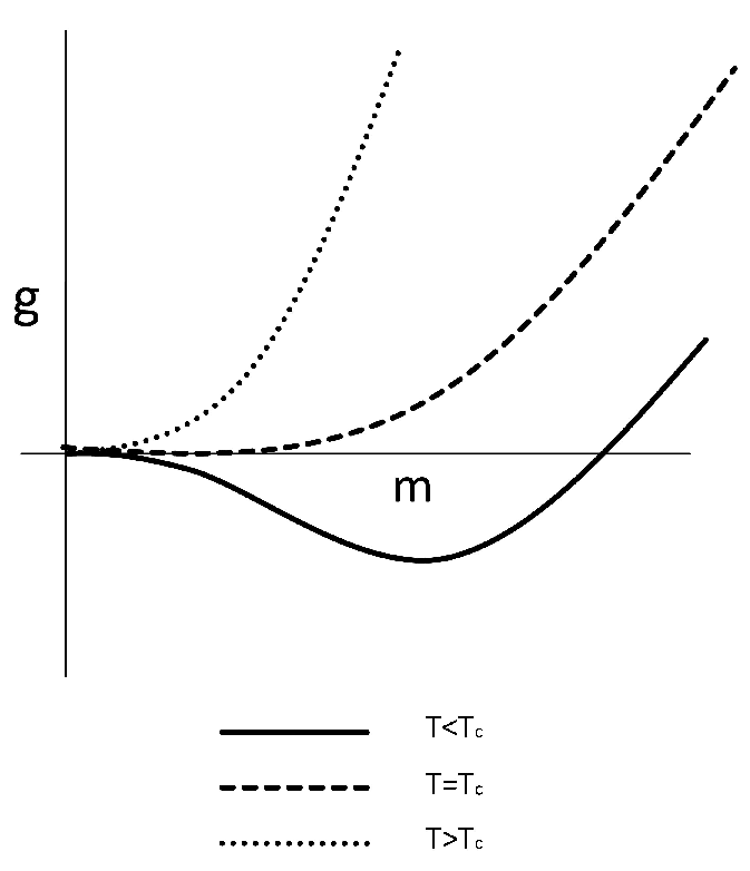
The typical $m$ -dependence of functions (3.6)–(3.8) at $h=0$ is shown in figure 1 (a). As it is common for the continuous phase transition scenario, the free energy has a single minimum (at $m=0$ ) for $T>T_{0}$ . A non-zero value of $m$ that minimizes the free energy appears starting from $T=T_{0}$ . In particular, the transition remains continuous in the percolation limit $q=1$ , as will be further considered in sections 3.2.1, 4.

Refer to caption — Figure 1: Typical behaviour of the free energy of the Potts model on uncorrelated scale-free networks at zero external field $h=0$ . (a): continuous phase transition; (b): first-order phase transition.

3.1.2 $q=2$

For $q=2$ , the Potts model corresponds to the Ising model. Indeed, in this case the coefficient at $m^{3}$ vanishes and the first terms in the free energy expansion read:

$\displaystyle 3<\lambda<5:$	$\displaystyle g=$	$\displaystyle\frac{A}{2T}(T-T_{0})m^{2}+K\frac{1}{T^{\lambda-2}}m^{\lambda-1}-\frac{D}{T}mh,$	(3.9)
$\displaystyle\lambda=5:$	$\displaystyle g=$	$\displaystyle\frac{A}{2T}(T-T_{0})m^{2}+\frac{C^{\prime}}{4T^{3}}m^{4}\ln{\frac{1}{m}}-\frac{D}{T}mh,$	(3.10)
$\displaystyle\lambda>5:$	$\displaystyle g=$	$\displaystyle\frac{A}{2T}(T-T_{0})m^{2}+\frac{C}{4T^{3}}m^{4}-\frac{D}{T}mh.$	(3.11)

It is easy to check that the above coefficients $K$ , $C$ , $C^{\prime}$ are positive for $q=2$ . Therefore, again the free energy behaviour corresponds to the continuous second-order phase transition, see figure 1 (a).

3.1.3 $q>2$

In this region of $q$ , phase transition scenario depends on the sign of the next-leading contribution to the free energy. Indeed, for positive $K$ the free energy reads:

3<\lambda<\lambda_{\mathrm{c}}(q):\hskip 10.00002ptg=\frac{A}{2T}(T-T_{0})m^{2}+K\frac{1}{T^{\lambda-2}}m^{\lambda-1}-\frac{D}{T}mh,

(3.12)

where $K$ remains positive in the region of $\lambda$ bounded by the marginal value $\lambda_{\mathrm{c}}$ defined by the condition

c(q,\lambda_{\mathrm{c}})=0\,,

(3.13)

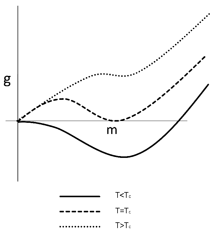
with $c(q,\lambda)$ given by (2.20). The free energy (3.12) is schematically shown in figure 1 (a) for different $T$ . As in the former cases, 3.1.1, 3.1.2, it corresponds to the continuous phase transition. With an increase of $\lambda$ , the coefficient $K$ becomes negative and one has to include the next term:

\lambda_{\mathrm{c}}(q)<\lambda<4:\hskip 10.00002ptg=\frac{A}{2T}(T-T_{0})m^{2}+K\frac{1}{T^{\lambda-2}}m^{\lambda-1}+\frac{B}{3T^{2}}m^{3}-\frac{D}{T}mh,

(3.14)

$B>0$ for $\lambda<4$ . Now, due to the negative sign of the coefficient at $m^{\lambda-1}$ , the free energy develops a local minimum for lower $T$ [see figure 1 (b)] and the order parameter manifests a discontinuity at the transition point $T_{\mathrm{c}}$ : scenario, typical of the first order phase transition. With further increase of $\lambda$ , one has to include more terms in the free energy expansion for the sake of thermodynamic stability. However, the sign at the second lowest order term remains negative, which corresponds to the free energy behaviour shown in figure 1 (b): the phase transition remains first order.

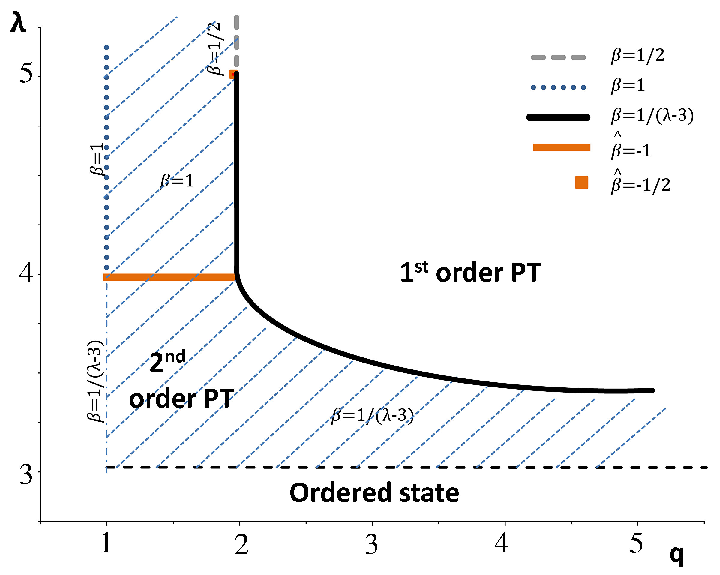
The above considerations can be summarized in the ‘‘phase diagram" of the Potts model on uncorrelated scale-free networks, that is shown in figure 2. Therein, we show the type of the phase transition for different values of parameters $\lambda$ and $q$ .

3.1.4 General $q$ , $2<\lambda\leqslant 3$

As it was outlined above, for $2<\lambda\leqslant 3$ the Potts model remains ordered at any finite temperature. Similar to the Ising model [27], it is easy to find the high-temperature decay of the order parameter in this region of $\lambda$ for any value of $q\geqslant 1$ . Since $\langle k^{2}\rangle$ becomes divergent for $2<\lambda\leqslant 3$ one does not write this term separately in the expression for the free energy [cf. (2.15)]. As a result, the corresponding expressions for the free energy read:

	$\displaystyle\hskip-20.00003pt2<\lambda<3:g=\frac{A}{2T}m^{2}+\frac{K^{\prime}}{T^{\lambda-2}}m^{\lambda-1}-\frac{D}{T}mh,$		(3.15)
	$\displaystyle\hskip-20.00003pt\lambda=3:g=\frac{A}{2T}m^{2}+\frac{c_{\lambda}J^{2}}{4q^{2}T}m^{2}\ln\frac{1}{m}+\frac{c_{\lambda}J^{2}}{T}\left[\frac{C^{\prime}(q,3)}{q-1}+\frac{1}{2q^{2}}\ln\left(\frac{Jk_{\star}}{T}\right)\right]m^{2}-\frac{D}{T}mh\,.$
			(3.16)

Here, the expressions for the coefficients $K^{\prime}$ , $C^{\prime}(q,3)$ are the same as for $K$ , $C(q,3)$ , equation (3.4), (2.25) with the only difference that the function $\varphi(x)$ used for their calculation does not contain the $x^{2}$ term. It is easy to check that the free energies (3.15), (3.16) are minimal for any finite temperature at a non-zero value of $m$ that decays at high $T$ as [32, 19]:

	$\displaystyle 2<\lambda<3:$		$\displaystyle m\sim T^{-\frac{\lambda-2}{3-\lambda}}\,,$		(3.17)
	$\displaystyle\lambda=3:$		$\displaystyle m\sim T\mathrm{e}^{-\alpha T},\hskip 10.00002pt\alpha>0\,.$		(3.18)

The above equations (3.17), (3.18) give the temperature behaviour of the mean-field order parameter $m$ . The connection with the magnetization $M$ is found from the self-consistency relation:

M=-\Big(\frac{\partial g}{\partial h}\Big)_{T}\,.

(3.19)

One can check that the solution of this equation at large $T$ is of the form $M\sim\frac{m}{T}$ . Correspondingly, this leads to the following high temperature decay of $M$ [27]:

	$\displaystyle 2<\lambda<3:$	$\displaystyle M\sim$	$\displaystyle T^{\frac{1}{\lambda-3}}\,,$		(3.20)
	$\displaystyle\lambda=3:$	$\displaystyle M\sim$	$\displaystyle\mathrm{e}^{-\alpha T},\hskip 10.00002pt\alpha>0\,.$		(3.21)

For the sake of simplicity, in what follows, we will express the thermodynamic functions in terms of the mean field order parameter $m$ . To get their $M$ dependence, one has to take into account the above considerations.

3.2 Regime of the second order phase transition, critical exponents

Let us find the critical exponents that govern the behaviour of thermodynamic functions in the vicinity of the 2nd order phase transition point $h=0$ , $\tau\equiv|T-T_{0}|/T_{0}=0$ ,where $T_{0}$ is the critical temperature of the 2nd order phase transition ( $T_{\mathrm{c}}^{\mathrm{2nd}}=T_{0}$ ). To this end, we will be interested in the following exponents that govern the temperature and field dependent behavior of the order parameter $m$ , the isothermal susceptibility $\chi_{T}=(\frac{\partial m}{\partial h})_{T}$ , the specific heat $c_{h}=T(\frac{\partial S}{\partial T})_{h}$ , and the magnetocaloric coefficient $m_{T}=-T(\frac{\partial S}{\partial h})_{T}$ :

	$\displaystyle h=0:$		$\displaystyle m\sim\tau^{\beta},\hskip 8.5359pt\chi_{T}\sim\tau^{-\gamma},\hskip 8.5359ptc_{h}\sim\tau^{-\alpha},\hskip 8.5359ptm_{T}\sim\tau^{-\omega},$		(3.22)
	$\displaystyle\tau=0:$		$\displaystyle m\sim h^{1/\delta},\hskip 8.5359pt\chi_{T}\sim h^{-\gamma_{\mathrm{c}}},\hskip 8.5359ptc_{h}\sim h^{-\alpha_{\mathrm{c}}},\hskip 8.5359ptm_{T}\sim h^{-\omega_{\mathrm{c}}}.$		(3.23)

Like in the previous subsection, we analyze this behaviour in different regions of $q$ and $\lambda$ . The results of this analysis are summarized in table 3.

Table 3: Leading critical exponents of the Potts model on uncorrelated scale-free network.

$q$	$\lambda$	$\alpha$	$\alpha_{\mathrm{c}}$	$\beta$	$\delta$	$\gamma$	$\gamma_{\mathrm{c}}$	$\omega$	$\omega_{\mathrm{c}}$
$1\leqslant q\leqslant 2$	$3<\lambda<4$	$\frac{\lambda-5}{\lambda-3}$	$\frac{\lambda-5}{\lambda-2}$	$\frac{1}{\lambda-3}$	$\lambda-2$	$1$	$\frac{\lambda-3}{\lambda-2}$	$\frac{\lambda-4}{\lambda-3}$	$\frac{\lambda-4}{\lambda-2}$
$1\leqslant q<2$	$\lambda\geqslant 4$	$-1$	$-1/2$	1	2	1	1/2	0	0
$q=2$	$3<\lambda<5$	$\frac{\lambda-5}{\lambda-3}$	$\frac{\lambda-5}{\lambda-2}$	$\frac{1}{\lambda-3}$	$\lambda-2$	$1$	$\frac{\lambda-3}{\lambda-2}$	$\frac{\lambda-4}{\lambda-3}$	$\frac{\lambda-4}{\lambda-2}$
$q=2$	$\lambda\geqslant 5$	0	0	1/2	3	1	2/3	1/2	1/3
$q>2$	$3<\lambda\leqslant\lambda_{\mathrm{c}}(q)$	$\frac{\lambda-5}{\lambda-3}$	$\frac{\lambda-5}{\lambda-2}$	$\frac{1}{\lambda-3}$	$\lambda-2$	$1$	$\frac{\lambda-3}{\lambda-2}$	$\frac{\lambda-4}{\lambda-3}$	$\frac{\lambda-4}{\lambda-2}$

3.2.1 $1\leqslant q<2$

In this region of $q$ , the free energy is given by the expressions (3.6)–(3.8). For $T>T_{0}$ , $g$ is minimal for $h=0$ at a zero value of the order parameter $m=0$ . For $T<T_{0}$ , the minimum of the free energy corresponds to the non-zero $m$ . Based on the expressions (3.6)–(3.8) we find in different regions of $\lambda$ :

$\displaystyle 3<\lambda<4:$	$\displaystyle m=$	$\displaystyle T_{0}^{\frac{\lambda-2}{\lambda-3}}\left[\frac{A\tau}{K(\lambda-1)}\right]^{\frac{1}{\lambda-3}},$	(3.24)
$\displaystyle\lambda=4:$	$\displaystyle m=$	$\displaystyle\frac{AT_{0}^{2}}{B^{\prime}}\tau\|\ln\tau\|^{-1},$	(3.25)
$\displaystyle\lambda>4:$	$\displaystyle m=$	$\displaystyle\frac{AT_{0}^{2}}{B}\tau.$	(3.26)

Using formulae (3.24), (3.26) at $q=1$ we reproduce the corresponding results for the percolation on scale-free networks [42]: the usual mean field percolation result for the exponent $\beta=1$ for $\lambda>4$ and $\beta=\frac{1}{\lambda-3}$ for $3<\lambda<4$ . Note the appearance of the logarithmic correction at the marginal value $\lambda=4$ . The resulting values of the exponent are given in table 3. Subsequently, we obtain the remaining exponents defined in (3.22), (3.23) and display them in the first two rows of table 3 as well.

Similar to the order parameter, (3.25), the temperature and field behaviour of the rest of thermodynamic functions at $\lambda=4$ in the vicinity of the critical point is characterized by the logarithmic corrections. Let us define the corresponding logarithmic-correction-to-scaling exponents by [47]:

	$\displaystyle h=0:\!\!\!$		$\displaystyle m\sim\tau^{\beta}{\mid\ln\tau\mid}^{\hat{\beta}},\quad\chi_{T}\sim\tau^{-\gamma}{\mid\ln\tau\mid}^{\hat{\gamma}},\hskip 8.5359ptc_{h}\sim\tau^{-\alpha}{\mid\ln\tau\mid}^{\hat{\alpha}},\quad m_{T}\sim\tau^{-\omega}{\mid\ln\tau\mid}^{\hat{\omega}},$		(3.27)
	$\displaystyle\tau=0:\!\!\!$		$\displaystyle m\sim h^{1/\delta}{\mid\ln h\mid}^{\hat{\delta}},\quad\chi_{T}\sim h^{-\gamma_{\mathrm{c}}}{\mid\ln h\mid}^{\hat{\gamma_{\mathrm{c}}}},\quad c_{h}\sim h^{-\alpha_{\mathrm{c}}}{\mid\ln h\mid}^{\hat{\alpha_{\mathrm{c}}}},\quad m_{T}\sim h^{-\omega_{\mathrm{c}}}{\mid\ln h\mid}^{\hat{\omega_{\mathrm{c}}}}\,.$		(3.28)

The obtained corresponding values are given in table 4. Note, that all exponents are negative: logarithmic corrections enhance the decay to zero of the decaying quantities and weaken the singularities of the diverging quantities. We discuss this behaviour more in detail in section 4.

Table 4: Logarithmic-corrections exponents for the Potts model on uncorellated scale-free network.

$q$	$\lambda$	$\hat{\alpha}$	$\hat{\alpha_{\mathrm{c}}}$	$\hat{\beta}$	$\hat{\delta}$	$\hat{\gamma}$	$\hat{\gamma_{\mathrm{c}}}$	$\hat{\omega}$	$\hat{\omega_{\mathrm{c}}}$
$1\leqslant q<2$	$\lambda=4$	$-2$	$-3/2$	$-1$	$-1/2$	0	$-1/2$	$-1$	$-1$
$q=2$	$\lambda=5$	$-1$	$-1$	$-1/2$	$-1/3$	0	$-1/3$	$-1/2$	$-2/3$

3.2.2 $q=2$ , the Ising model

For different $\lambda$ , the free energy is given by (3.9)–(3.11). Minimizing these expressions one finds for the order parameter at $h=0$ , $T<T_{0}$ :

$\displaystyle 3<\lambda<5:$	$\displaystyle m=$	$\displaystyle T_{0}^{\frac{\lambda-2}{\lambda-3}}\left[\frac{A\tau}{K(\lambda-1)}\right]^{\frac{1}{\lambda-3}},$	(3.29)
$\displaystyle\lambda=5:$	$\displaystyle m=$	$\displaystyle\sqrt{\frac{AT_{0}^{3}}{C^{\prime}}}\tau^{1/2}\|\ln\tau\|^{-1/2},$	(3.30)
$\displaystyle\lambda>5:$	$\displaystyle m=$	$\displaystyle\sqrt{\frac{AT_{0}^{3}}{C}}\tau^{1/2}.$	(3.31)

The corresponding critical exponents for the other thermodynamic quantities are given in the third and fourth rows of table 3. Logarithmic corrections to scaling (3.27)–(3.28) appear at $\lambda=5$ , their values are given in the second row of table 4. Critical behaviour of this model on an uncorrelated scale-free network was a subject of intensive analysis, see e.g., the papers [32, 27, 28, 31] and by the result given in table 3 we reproduce the results for the exponents obtained therein.

3.2.3 $q>2$ , $3<\lambda\leqslant\lambda_{\mathrm{c}}(q)$

In this region of $q,\,\lambda$ the phase transition remains continuous, see the phase diagram, figure 2, and the free energy is given by the expression (3.12). Correspondingly, one finds that the spontaneous magnetization behaves as

3<\lambda\leqslant\lambda_{\mathrm{c}}(q):\,\,m=T_{0}^{\frac{\lambda-2}{\lambda-3}}\left[\frac{A\tau}{K(\lambda-1)}\right]^{\frac{1}{\lambda-3}}.

(3.32)

The values of the rest of the critical exponents are given in the sixth row of table 3. Since the leading terms of the free energy (3.12) at $3<\lambda\leqslant\lambda_{\mathrm{c}}(q)$ coincide with that of the Ising model at $3<\lambda\leqslant 5$ , (3.9), the behaviour of thermodynamic functions in the vicinity of the second order phase transition is governed by the same set of the critical exponents: the Potts model for $q>2$ , $3<\lambda\leqslant\lambda_{\mathrm{c}}(q)$ belongs to the universality class of the Ising model at $3<\lambda\leqslant 5$ . This result was first observed in [19] by treating the mean field approximation for the equation of state.

3.3 The first order phase transition

For $q>2$ , $\lambda>\lambda_{\mathrm{c}}(q)$ the phase transition is of the first order, see the phase diagram in figure 2. As we have outlined in section 3.1.3, the next-leading order term of the free energy has a negative sign and the free energy behaves as shown in figure 1 (b). As further analysis shows, the higher the value of $\lambda$ the more terms one has to take into account in the free energy expansion in order to ensure the correct $g(m)$ asymptotics. Therefore, in the results given below we restrict ourselves to the region $\lambda_{\mathrm{c}}(q)<\lambda<4$ , where the free energy is given by equation (3.14). The first order phase transition temperature $T_{\mathrm{c}}^{\mathrm{1st}}$ is found from the condition $g(m=0,{T_{\mathrm{c}}^{\mathrm{1st}}})=g(m\neq 0,{T_{\mathrm{c}}^{\mathrm{1st}}})$ , see the red (middle) curve in figure 1 (b):

{T_{\mathrm{c}}^{\mathrm{1st}}}=T_{0}+\left[\frac{-B}{3K(\lambda-1)(\lambda-3)}\right]^{\frac{\lambda-3}{\lambda-4}}\frac{2K(\lambda-1)(\lambda-4)}{A}\,.

(3.33)

For the jump of the order parameter $\Delta m$ at $T_{\mathrm{c}}$ we find:

\Delta m=\left[\frac{-B}{3K(\lambda-1)(\lambda-3)}\right]^{\frac{1}{\lambda-4}}\,.

(3.34)

Another thermodynamics function to characterize the first order phase transition is the latent heat $Q$ . It is defined by:

Q=\Delta S\cdot{T_{\mathrm{c}}^{\mathrm{1st}}}\,,

(3.35)

where $\Delta S$ is the jump of entropy at $T_{\mathrm{c}}$ . With the free energy given by (3.14) we find the entropy as

S=-\Big(\frac{\partial g}{\partial T}\Big)_{h,m}\,.

(3.36)

Considering the entropy at the transition temperature we can find the latent heat at the first order phase transition for $\lambda_{\mathrm{c}}(q)<\lambda<4$ :

Q=\frac{A}{2}(\Delta m)^{2}.

(3.37)

4 Notes about percolation on scale-free networks

By the results of section 3.2.1 we also cover the case $q=1$ , which corresponds to percolation on uncorrelated scale-free networks. The ‘‘magnetic’’ exponents governing corresponding second order phase transition are given in tables 3, 4. Let us discuss them more in detail, in particular relating them to percolation exponents. The following exponents are usually introduced to describe the behavior of different observables near the percolation ⁵⁵ 5 For definiteness, let us consider the site percolation and denote by $p$ here and below the site occupation probability. point $p_{\mathrm{c}}$ [51, 52]: the probability that a given site belongs to the spanning cluster

P_{\infty}\sim(p-p_{\mathrm{c}})^{\beta},\qquad p>p_{\mathrm{c}}\,,

(4.1)

the number of clusters of size $s$

n_{s}\sim s^{-\tau}\mathrm{e}^{-s/s^{*}},

(4.2)

the cluster size at criticality

s^{*}\sim|p-p_{\mathrm{c}}|^{-\sigma},

(4.3)

the average size of finite clusters

\langle s\rangle\sim|p-p_{\mathrm{c}}|^{-\gamma}.

(4.4)

The above defined exponents $\beta$ and $\gamma$ coincide with the ‘‘magnetic’’ exponents $\beta$ and $\gamma$ of the $q=1$ Potts model (see tables 3, 4). Therefore, the probability that a given site belongs to the spanning cluster, and the average size of finite clusters for percolation on uncorrelated scale-free networks are governed by the scaling exponents:

\beta=\left\{\begin{array}[]{cc}\frac{1}{\lambda-3},&\hskip 28.45274pt3<\lambda<4,\\ 1,&\hskip 28.45274pt\lambda>4,\end{array}\right.

(4.5)

\gamma=1,\hskip 28.45274pt\lambda>3.

(4.6)

The exponents $\tau$ and $\sigma$ may be derived with the help of familiar scaling relations [51, 52]:

\sigma\beta=\tau-2,

(4.7)

\gamma=\frac{3-\tau}{\sigma}\,.

(4.8)

Substituting the values of $\beta$ and $\gamma$ (4.5), (4.6) into (4.7), (4.8) one arrives at the following expressions for the exponents $\tau$ and $\sigma$ :

\tau=\left\{\begin{array}[]{cc}\frac{2\lambda-3}{\lambda-2},&\hskip 28.45274pt3<\lambda<4,\\ \frac{5}{2},&\hskip 28.45274pt\lambda>4,\end{array}\right.

(4.9)

\sigma=\left\{\begin{array}[]{cc}\frac{\lambda-3}{\lambda-2},&\hskip 28.45274pt3<\lambda<4,\\ 1/2,&\hskip 28.45274pt\lambda>4.\end{array}\right.

(4.10)

Analysing the high-temperature behaviour of the Potts model magnetization at $2<\lambda<3$ , (3.20), one arrives at the scaling exponents $\beta=1/(3-\lambda)$ , $\gamma=-1$ for the corresponding observables for percolation at $p_{\mathrm{c}}=0$ .

Our formulas (4.5), (4.6), (4.9), and (4.10) reproduce the results for the scaling exponents that govern percolation on uncorrelated scale-free networks [43, 42] as well as those found for the related models of virus spreading [44, 45]. All the above mentioned papers do not explicitly discuss the case $\lambda=4$ and possible logarithmic corrections that arise therein. Moreover, a recent review [46], that also discusses the peculiarities of percolation on uncorrelated scale-free networks does not report on logarithmic corrections [its equation (95) is perhaps wrong since it gives no logarithmic corrections for $\lambda=4$ .] Our results are in the first row of table 4 where we give a comprehensive list of critical exponents that govern logarithmic corrections to scaling appearing for the Potts model at $q=1$ , $\lambda=4$ , as correctly predicted within the general Landau theory for systems of arbitrary symmetry on uncorrelated scale-free networks [53]. One may compare our values with the corresponding exponents of the $d$ -dimensional lattice percolation at $d=6$ : $\hat{\alpha}=\hat{\beta}=\hat{\gamma}=\hat{\delta}=\hat{\alpha}_{\mathrm{c}}=2/7$ (see e.g. [47]). In this respect, the logarithmic-correction exponents for the lattice percolation at $d=6$ and for the scale-free network percolation at $\lambda=4$ belong to different universality classes. It is easy to check that the exponents quoted in the last row of table 4 obey the scaling relations for the logarithmic-corrections exponents: $\hat{\beta}(\delta-1)=\delta\hat{\delta}-\hat{\gamma}$ , $\hat{\alpha}=2\hat{\beta}-\hat{\gamma}$ [48, 49, 50], $\hat{\gamma_{\mathrm{c}}}=\hat{\delta}$ , $\hat{\alpha_{\mathrm{c}}}=\frac{(\gamma+2)(\hat{\beta}-\hat{\gamma})}{\beta+\gamma}+\hat{\gamma}$ [28].

5 Conclusions and outlook

In this paper we have analyzed the critical behaviour of the $q$ -state Potts model on an uncorrelated scale-free network. The mean field approach we use in our calculations often leads to asymptotically exact results when critical behaviour on an uncorrelated scale-free network is considered. However, in the case of the Potts model, two similar approximate schemes of calculations, the mean field [19] and the recurrent relations for the tree-like random graphs [20] differ in their results concerning the phase diagram. In particular, for $q>2$ and $\lambda\leqslant 3$ , both approaches predict that the system always remains ordered at finite temperature. However, for $\lambda>3$ , depending on specific values of $\lambda$ , the first approach predicts the first or the second order phase transition, whereas the second approach predicts the first order phase transition. Our results complete the above analysis. However, unlike [19], where the equation of state was considered, we have considered the thermodynamic potential which enabled us to present a comprehensive analysis of temperature and magnetic field dependence of thermodynamic quantities. It is worth noting that the model considered here is alike the Hopfield model [34, 35, 36, 37], for which the mean field approximation is known to give exact results.

Our main results are summarized in figure 2 and in tables 3, 4. Depending on the values of $q$ and on the node degree distribution exponent $\lambda$ , the Potts model manifests either the first-order or the second-order phase transition or it is ordered at any finite temperature, see figure 2. In the second order phase transition region (shaded in the figure), it belongs either to the universality class of the Ising model on an uncorrelated scale-free network (with $\lambda$ -dependent critical exponents) or it is governed by the mean field percolation ( $1\leqslant q<2$ , $\lambda\geqslant 4$ ) or mean field Ising ( $q=2$ , $\lambda\geqslant 5$ ) exponents.

One of the major points where the critical behaviour of the Potts model in the second order phase transition regime differs from the Ising model is that its logarithmic correction exponents belong to two different universality classes. As it is well known, in certain situations, the scaling behaviour is modified by multiplicative logarithmic corrections (see [47] for a recent review and [54] for the specific case of the Potts model). For lattice systems, such corrections are known to appear, in particular, at the so-called upper critical dimension, above which the mean field regime holds. For the scale-free networks, where the very notion of dimensionality is ill-defined, a change in the node degree distribution exponent $\lambda$ may turn a system to such a regime. For the Ising model, this happens at $\lambda=5$ and is caused by the divergencies in the fourth moment of the node degree distribution $\langle k^{4}\rangle$ , as it was analyzed in detail in [28]. In addition to these corrections, for the Potts model we observe an onset of multiplicative corrections to scaling at $1\leqslant q<2$ for $\lambda=4$ . Contrary to the Ising case, these are caused by the divergencies in the third moment of the node degree distribution $\langle k^{3}\rangle$ . This difference in the origin of the appearance of these corrections also causes the difference in their numerical values: this new set of the logarithmic correction to scaling exponents belongs to the new universality class. In particular, they govern percolation on uncorrelated scale-free networks at $\lambda=4$ .

Acknowledgements

It is our pleasure to thank Bernat Corominas-Murtra, Yuri Kozitsky, Volodymyr Tkachuk, and Loïc Turban for useful discussions. This work was supported in part by the 7th FP, IRSES project N269139 ‘‘Dynamics and Cooperative phenomena in complex physical and biological environments".

References

[1] Albert R., Barabasi A.-L., Rev. Mod. Phys., 2002, 74, 47; doi:10.1103/RevModPhys.74.47.
[2] Dorogovtsev S.N., Mendes J.F.F., Evolution of Networks: From Biological Networks to the Internet and WWW, Oxford University Press, 2003.
[3] Holovatch Yu., von Ferber C., Olemskoi A., Holovatch T., Mryglod O., Olemskoi I., Palchykov V., J. Phys. Stud., 2006, 10, 247 (in Ukrainian).
[4] Barrat A., Barthelemy M., Vespignani A., Dynamical Processes on Complex Networks, Cambridge University Press, 2008.
[5] Newman M., Networks: An Introduction, Oxford University Press, 2010.
[6] Dorogovtsev S. N., Goltsev A. V., Rev. Mod. Phys., 2008, 80, 1275; doi:10.1103/RevModPhys.80.1275.
[7] Galam S., Sociophysics: A Physicist’s Modeling of Psycho-political Phenomena (Understanding Complex Systems), Springer, New York, Dordrecht, Heidelberg, London, 2012.
[8] Tadić B., Malarz K., Kułakowski K., Phys. Rev. Lett., 2005, 94, 137204; doi:10.1103/PhysRevLett.94.137204.
[9] Wu F.Y., Rev. Mod. Phys., 1982, 54, 235; doi:10.1103/RevModPhys.54.235.
[10] Berche B., Chatelain C. Phase Transitions in Two-Dimensional Random Potts Models, In: Order, Disorder and Criticality Advanced Problems of Phase Transition Theory, Yu. Holovatch (Ed.), World Scientific, Singapore, 2004, 147–200.
[11] Chatelain C., Berche B., Janke W., Berche P.-E., Nucl. Phys. B, 2005, 719, 275; doi:10.1016/j.nuclphysb.2005.05.003.
[12] Müller-Hartmann E., Zittartz J., Phys. Rev. Lett., 1974, 33, 893; doi:10.1103/PhysRevLett.33.893.
[13] Müller-Hartmann E., Zittartz J., Z. Physik, 1975, 22, 59.
[14] Wang Y.K., Wu F.Y., J. Phys. A, 1976, 9, 593; doi:10.1088/0305-4470/9/4/016.
[15] Turban L., Phys. Lett. A, 1980, 78, 404; doi:10.1016/0375-9601(80)90408-9.
[16] Ganikhodjaev N., Mukhamedov F., Mendes J.F.F., J. Stat. Mech., 2006, P08012; doi:10.1088/1742-5468/2006/08/P08012.
[17] Ganikhodjaev N., Mukhamedov F., Pah C.H., Phys. Lett. A, 2008, 373, 33; doi:10.1016/j.physleta.2008.10.060.
[18] Araújo N. A. M., Andrade R. F. S., Herrmann H. J., Phys. Rev. E, 2010, 82, 046109; doi:10.1103/PhysRevE.82.046109.
[19] Iglói F., Turban L.. Phys. Rev. E, 2002, 66, 036140; doi:10.1103/PhysRevE.66.036140.
[20] Dorogovtsev S., Goltsev A.V., Mendes J.F.F., Eur. Phys. J. B, 2004, 38, 177; doi:10.1140/epjb/e2004-00019-y.
[21] Ehrhardt G.C.M.A., Marsili M., J. Stat. Mech., 2005, P02006; doi:10.1088/1742-5468/2005/02/P02006.
[22] Shen C., Chen H., Hou Z., Xin H., Phys. Rev. E, 2011, 83, 066109; doi:10.1103/PhysRevE.83.066109.
[23] Khajeh E., Dorogovtsev S.N., Mendes J.F.F., Phys. Rev. E, 2007, 75, 041112; doi:10.1103/PhysRevE.75.041112.
[24] Hooyberghs H., van Schaeybroeck B., Moreira A.A., Andrade J.S. (Jr.), Herrmann H.J., Indekeu J.O., Phys. Rev. E, 2010, 81, 011102; doi:10.1103/PhysRevE.81.011102.
[25] Karsai M., Anglès d’Auriac J.-Ch., F. Iglói F., Phys. Rev. E, 2007, 76, 041107; doi:10.1103/PhysRevE.76.041107.
[26] Bender E.A., Canfield E.R., J. Comb. Theory A, 1978, 24, 296; doi:10.1016/0097-3165(78)90059-6.
[27] Dorogovtsev S.N., Goltsev A.V., Mendes J.F.F., Phys. Rev. E, 2002, 66, 016104; doi:10.1103/PhysRevE.66.016104.
[28] Palchykov V., von Ferber C., Folk R., Holovatch Yu., Kenna R., Phys. Rev. E, 2010, 82, 011145; doi:10.1103/PhysRevE.82.011145.
[29] Suchecki K., Hołyst J. A., Phys. Rev. E, 2006, 74, 011122; doi:10.1103/PhysRevE.74.011122.
[30] Suchecki K., Hołyst J. A., Phys. Rev. E, 2009, 80, 031110; doi:10.1103/PhysRevE.80.031110.
[31] von Ferber C., Folk R., Holovatch Yu., Kenna R., Palchykov V., Phys. Rev. E, 2011, 83, 061114; doi:10.1103/PhysRevE.83.061114.
[32] Leone M., Vázquez A., Vespignani A., Zecchina R., Eur. Phys. J. B, 2002, 28, 191; doi:10.1140/epjb/e2002-00220-0.
[33] Suchecki K., Hołyst J.A., In: Order, Disorder and Criticality Advanced Problems of Phase Transition Theory, Vol. 3, Yu. Holovatch (Ed.), World Scientific, Singapore, 2012, p. 167–201.
[34] Pastur L.A., Figotin A.L., Theor. Math. Phys., 1978, 35, 403; doi:10.1007/BF01039111.
[35] Hopfield J.J., Proc. Natl. Acad. Sci. U.S.A., 1982, 79, 2554; doi:10.1073/pnas.79.8.2554.
[36] Gayrard V., J. Stat. Phys., 1992, 68, 977; doi:10.1007/BF01048882.
[37] Bovier A., Gayrard V., Picco P., Probab. Theory Rel., 1995, 101, 511; doi:10.1007/BF01202783.
[38] Bianconi G., Phys. Lett. A, 2002, 303, 166; doi:10.1016/S0375-9601(02)01232-X.
[39] Fernández Sabido S. F., Applications exploratoires des modèles de spins au Traitement Automatique de la Langue. PhD Thesis, University Henri Poincaré, Nancy I, Nancy, France, 2009.
[40] Aiello W., Park F., Lu L., In: Proceeding STOC’00 Proceedings of the thirty-second annual ACM symposium on Theory of computing (Portland, 2000), ACM New York, 2000, p. 171–180.
[41] Bender E.A., Steven A.O., Advanced Mathematical Methods for Scientists and Engineers, McGraw-Hill, 1978.
[42] Cohen R., ben-Avraham D., Havlin S., Phys. Rev. E, 2002, 66, 036113; doi:10.1103/PhysRevE.66.036113.
[43] Cohen R., Erez K., ben-Avraham D., Havlin S., Phys. Rev. Lett., 2001, 86, 3682; doi:10.1103/PhysRevLett.86.3682.
[44] Pastor-Satorras R., Vespignani A., Phys. Rev. E, 2001, 63, 066117; doi:10.1103/PhysRevE.63.066117.
[45] Moreno Y., Pastor-Satorras R., Vespignani A., preprint arXiv:cond-mat/0107267, 2001.
[46] Hasegawa T., Interdisc. Inf. Sci., 2011, 17, 175.
[47] Kenna R., In: Order, Disorder and Criticality Advanced Problems of Phase Transition Theory, Vol. 3, Yu. Holovatch (Ed.), World Scientific, Singapore, 2012, p. 1–47.
[48] Kenna R., Johnston D. A., Janke W., Phys. Rev. Lett., 2006, 96, 115701; doi:10.1103/PhysRevLett.96.115701.
[49] Kenna R., Johnston D. A., Janke W., Phys. Rev. Lett., 2006, 97, 155702; doi:10.1103/PhysRevLett.97.155702.
[50] Kenna R., Johnston D. A., Janke W., Phys. Rev. Lett., 2006, 97, 169901E; doi:10.1103/PhysRevLett.97.169901.
[51] Essam J. W., Rep. Prog. Phys., 1980, 43, 833; doi:10.1088/0034-4885/43/7/001.
[52] Stauffer D., Aharony A., Introduction to Percolation Theory, Taylor & Francis, London, 1991.
[53] Goltsev A. V., Dorogovtsev S. N., Mendes J.F.F., Phys. Rev. E, 2003, 67, 026123; doi:10.1103/PhysRevE.67.026123.
[54] Berche B., Butera P., Shchur L., J. Phys. A: Math. Theor., 2013, 46, 095001; doi:10.1088/1751-8113/46/9/095001.

Критична поведiнка моделi Поттса на складних мережах

М. Красницька^?,?, Б. Берш ${}^{\textsf{\footnotesize{\mbox{?}}}}$ , Ю. Головач ${}^{\textsf{\footnotesize{\mbox{?}}}}$

${}^{\textsf{\footnotesize 1}}$

нститут фзики конденсованих систем НАН Украни,
вул. Свнццького, 1, 79011 Львв, Украна
${}^{\textsf{\footnotesize 2}}$

Iнститут Ж. Лямура, Унiверситет Лотаринг, F–54506 Вандевр-ле-Нанс, Францiя

Phase transitions in the Potts model on complex networks

Abstract

1 Introduction

2 Free energy of the Potts model on uncorrelated scale-free network

2.1 General relations

2.2 Non-integer λ\lambda

2.3 Integer λ\lambda

3 Thermodynamic functions

3.1 The phase diagram

3.1.1 1⩽q<21\leqslant q<2

3.1.2 q=2q=2

3.1.3 q>2q>2

3.1.4 General qq, 2<λ⩽32<\lambda\leqslant 3