Gapless interface states at the junction between two topological insulators

The low energy physics of a bulk strong TI, like Bi₂Se₃, is described up to order $k^{2}$ by the effective Hamiltonian [9, 20]

where $\bm{\sigma}$ are the Pauli matrices for the Bi and Se sites, and

with $\bm{k}=(k_{x},k_{y})$ and $k_{\pm}=k_{x}\pm ik_{y}$. The Schrödinger equation is given by $\mathcal{H}\Phi=E\Phi$, where $\Phi=\left(\mbox{Bi}_{\uparrow},\mbox{Se}_{\uparrow},\mbox{Bi}_{\downarrow},\mbox{Se}_{\downarrow}\right)$ gives the amplitude of the spin-orbit coupled $p_{z}$ orbitals that mainly contribute to the low energy physics of Bi₂Se₃. The band inversion which characterizes the topological phase, is determined by the condition $M_{0}M_{1}<0$ (Ref. 20).

Surface states obtained from this model have linear dispersion near the $\Gamma$ point with Fermi velocity $v=(|A|/\hbar)\left[1-(C_{1}/M_{1})^{2}\right]^{1/2}$, and a helical spin texture [22]. The helicity direction of the spin texture depends on the relative sign of the parameters $A$ and $B$, i.e. $\left<s_{x,y}\right>\sim\mathop{\rm sgn}\nolimits\left({AB}\right)k_{y,x}$ (Ref. 20).

We consider a junction at $z=0$ between two TIs, TI1 ($z<0$) and TI2 ($z>0$) (Fig. 1). The junction breaks translation symmetry in the $z$-direction, and we let $k_{z}\rightarrow-i\partial_{z}$ to obtain a system of second order homogeneous differential equations $\mathcal{H}(\bm{k},-i\partial_{z})\Phi=E\Phi$ with $\Phi=e^{i\bm{k}\cdot\bm{\rho}}\bm{\phi}(z)$. This is solved with the ansatz $\bm{\phi}(z)\sim e^{\lambda z}\Psi(E,\bm{k})$, where $\Psi(E,\bm{k})$ is an eigenvector of the Hamiltonian. We obtain a system of algebraic equations that has a nonzero solution if $|\mathcal{H}(\bm{k},-i\lambda)-E|=0$. Details on the solution method are given in the Appendix. Solving for $\lambda$ yields four doubly degenerate $\lambda_{\alpha}(E,\bm{k})$ $(\alpha=1,\ldots,4)$ in general, each corresponding to two eigenvectors $\Psi_{s,\alpha}$ $(s=1,2)$ (Eq. (7)). The total solution is then given by the linear combination

where the coefficients $C_{s,\alpha}(E,\bm{k})$ are found from the boundary conditions.

We want to study states localized at the junction, and therefore we only consider the two $\lambda^{(m)}$ with Re $\lambda^{(1)}>0$ for TI1 and Re $\lambda^{(2)}<0$ for TI2, to construct the wave function (2) (see Eq. (6)). Here $m$ labels TI1 and TI2 respectively. The remaining boundary conditions are given by the continuity of the wave function and the current at the junction [23]

The nonzero solutions $C_{s,\alpha}^{(m)}(E,\bm{k})\neq 0$ of this system of homogeneous equations, define the dispersion and wave functions of the interface states. We numerically solved this system on a $(E,\bm{k})$ grid by means of the condition number and singular value decomposition of the coefficient matrix.

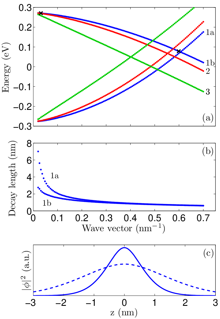
First we consider the case where $B^{(2)}=B^{(1)}$ and $A^{(1)}A^{(2)}<0$. This corresponds with TIs that have surface states with opposite helicity direction (Fig. 1), and the magnitude of $A^{(1,2)}$ determines the Fermi velocity of the surface states. In Fig. 2(a) the dispersion of the interface states is shown for three different values of $A^{(2)}$. The interface states have linear dispersion (in the radial direction) around $k\neq 0$ which results from the hybridization of the Dirac cones from the separated TIs, similar to AA stacked bilayer graphene [24]. The cones intersect closer to the center if their Fermi velocity is smaller. From the energy scale in Fig. 2(a) one can see that the conduction/valence band of the cone is pushed into the bulk region of the band structure, which has a band gap around $0.3$ eV [9, 11]. Correspondingly, as the bands approach $k=0$, the decay length $\equiv\max\left(1/|\mbox{Re}~\lambda_{\alpha}|\right)$ diverges exponentially, as shown in Fig. 2(b).

The total density near the junction is shown in Fig. 2(c) for a state close to the crossing point and a state close to the bulk region. Both states are marked with a cross in Fig. 2(a). We see that the character of the individual surface states is completely lost and the interface states are spread over the entire junction.

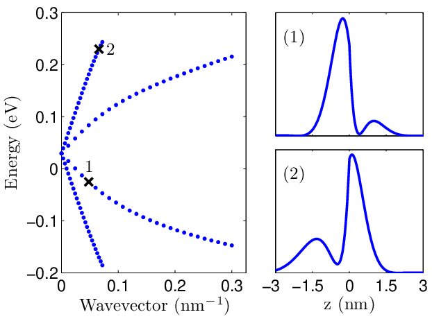
Next we consider the case where $B^{(1)}B^{(2)}<0$ and $A^{(1)}A^{(2)}>0$. Again this corresponds with TIs that have surface states with opposite helicity direction (Fig.1), and the magnitude of $A^{(1,2)}$ determines the Fermi velocity of the surface states. In Fig. 3 the dispersion of the interface states is shown for $B^{(2)}=-B^{(1)}$ and $A^{(2)}=10A^{(1)}$. Unlike case 1, there is little interaction between the surfaces, and the cones lie on top of each other.

The density is also shown for two states in Fig. 3, one on each cone. We see that the states on each cone are not localized at the junction, but instead they are localized inside one of the TIs, as we would expect if there is little interaction, and the individual surface states keep most of their original character. TI2 has the largest Fermi velocity, correspondingly the states on the steepest cone are localized in TI2. The Fermi velocity of the cones in the interface spectrum is two times as large as the original cone of the separated TI for TI1 and about 0.8 times smaller for TI2, and thus the cones are attracted to each other.

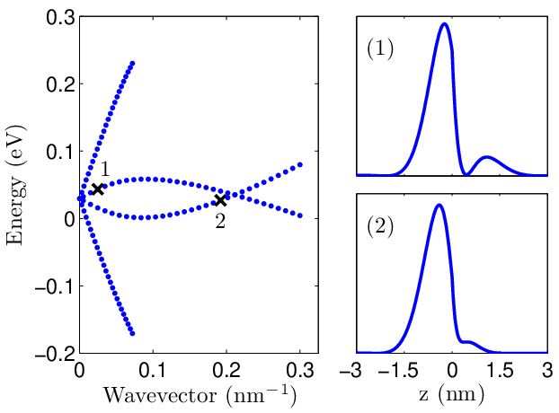
Finally we consider the case where $B^{(1)}B^{(2)}<0$ and $A^{(1)}A^{(2)}<0$. Unlike the previous two cases, this corresponds with TIs that have surface states with equal helicity direction. The dispersion of the interface states is shown in Fig. 4 for $B^{(2)}=-B^{(1)}$ and $A^{(2)}=-10A^{(1)}$. We see that we get a combination of the previous two cases, a linear spectrum near the center and a crossing away from the center. The density is also shown for two states in Fig. 4, localized on TI1, one near the center and one near the crossing point. We see that near the center, we have the same behavior as in case 2, and closer to the crossing point the interaction between the surfaces is stronger as indicated by the shift of the density towards the junction. The states on the steep cone do not differ much from those of the steep cone of Fig. 3 and are localized within TI2.

If the helicity direction of the TIs is opposite, the existence of the gapless interface states can be understood from scattering of surface states at the junction between the two TIs, as shown in Refs. 19 and 25. At normal incidence, the incoming state on the surface of TI1 cannot scatter backwards because of spin conservation. This is similar to graphene, where pseudospin conservation results in Klein tunneling through potential barriers at normal incidence [26]. However, when TI2 has opposite helicity, the incoming state cannot go forward because there are no states in TI2 that conserve both spin and momentum. This paradox is solved by the existence of gapless interface states between the TIs. At normal incidence the incoming state has to go into the interface. Consequently, these states should exist for $k_{x}=0$ or $k_{y}=0$.

The origin of the surface states in TIs can be understood from the closure of the bulk band gap if the Hamiltonian is transformed continuously from a trivial insulator to a TI. In the same way, we can understand the interface states at the junction between two TIs. We observe that the gap of the bulk band structure of the Hamiltonian (1) closes at $k\neq 0$ if the parameter $A$ changes sign, and it closes at $k=0$ if the parameter $B$ changes sign, which could be an indication of a topological phase transition. The origin of the interface states within the model can then also be understood from this closing of the bulk gap when $A=0$ at $k\neq 0$ for case 1, and when $B=0$ at $k=0$ for case 2. When both parameters $A$ and $B$ change sign as in case 3, we end up with two TIs with equal helicity direction. Therefore, at first sight it might be surprising that interface states appear. However, from the previous discussion it is clear that the bulk gap closes at two different $k$ values when both $A$ and $B$ change sign, which explains why the resulting spectrum in case 3 (Fig. 4) is a combination of the spectra of case 1 (Fig. 2(a)) and case 2 (Fig. 3). This is illustrated with a schematic phase diagram in Fig. 5, where we show the four different sign combinations of $A$ and $B$, and the $(k,k_{z})$ points at which the gap closes when the helicity changes orientation.

Because of the invariance of the Hamiltonian (1) under any rotation about the $z$-axis, we find gapless interface states along any $\bm{k}$-direction. If we take into account terms up to order $k^{3}$, the full rotation symmetry is relaxed to threefold $C_{3}$ rotation symmetry of the Bi₂Se₃ crystal [20], and we expect a gap to open in the interface spectrum along $k_{x}\neq 0$ or $k_{y}\neq 0$ directions, giving a total of six Dirac cones over the entire Brillouin zone. However, the solution method becomes unpractical in this case, because the equation for $\lambda$ (6) contains odd powers, and we need to find the roots of a depressed quartic equation.

Now raises the question if materials can exist for which the parameters $A$ and $B$ changes sign with respect to their Bi₂Se₃ values. In Ref. 20 it is argued that the sign of $A$ is determined by the sign of the atomic SOC, while the sign of $B$ is independent of the atomic SOC. However, the atomic SOC parameter, given by the diagonal matrix element of $\hat{H}_{SO}=(2m_{e}^{2}c^{2}r)^{-1}(\partial U/\partial r)\bm{L}\cdot\bm{S}$, does not change sign for Bi₂Se₃-like TIs because the potential is always attractive for atoms [20]. Therefore, the helicity direction is always the same within the Bi₂Se₃ family of TIs. However, the model (1) is valid for a general TI, and therefore we believe that the interface between TIs with opposite helicity is possible in principle, as was also mentioned in Ref. 19. Furthermore, there are other mechanisms besides SOC which can give rise to a band inversion. For example, strained bulk HgTe is a 3D TI [27] in which the band inversion is caused by other relativistic corrections [28]. Also in type-II InAs/GaSb heterostructures, one can achieve a band inversion from confinement [29].

We found no signature of tachyons in this system as claimed in Ref. 21. The reason is the following. If the $\lambda$’s used to construct the general solution (2) become four times degenerate, the solution is no longer valid because it contains the same contribution twice. In this case, the matrix of the homogeneous system, defined by the boundary conditions (3), is always singular and one seemingly finds solutions. The extra degeneracy occurs at $(E,\bm{k})$ points where the equation in $\lambda^{2}$ has a repeated root (Eq. (6)). This happens when the discriminant vanishes which allowed us to obtain an expression for the ‘dispersion’,

with

When the argument of the square root becomes negative, the ‘group velocity’ diverges and $E_{t}$ becomes complex. This happens at $f(k_{t})=0$, which gives the tachyonic point [21]

In Fig. 6 we show the dispersion for the case which was also considered in Ref. 21, $A^{(2)}=-A^{(1)}$ and $B^{(2)}=3.0$ eVÅ. We see that Eq. (4) exactly fits the tachyonlike ‘dispersions’ obtained with a numerical calculation that does not take the degeneracy into account. In this case we get two tachyonlike ‘dispersions’ because the degeneracy occurs for $\lambda^{(1)}$ and $\lambda^{(2)}$ for this parameter set. We know that the degeneracy occurs on a real $(E,k)$ grid if $k_{t}$ is real. The same problem occurs if we consider a vacuum interface, because the degeneracy of $\lambda$ is independent of the boundary conditions. In this case, one can analytically show that the tachyonic solutions are not physical.

The correct general solution at the degeneracy is given by Eq. (11) in the Appendix. Now we only find solutions at the points of intersection between the unphysical tachyonlike ‘dispersion’ and physical solutions.

References

- [1] C. L. Kane and E. J. Mele, Phys. Rev. Lett. 95, 146802 (2005).
- [2] B. A. Bernevig, T. L. Hughes, and S. C. Zhang, Science 314, 1757 (2006).
- [3] M. König, S. Wiedmann, C. Brüne, A. Roth, H. Buhman, L. W. Molenkamp, X. L. Qi, and S. C. Zhang, Science 318, 766 (2007).
- [4] L. Fu, C. L. Kane, and E. J. Mele, Phys. Rev. Lett. 98, 106803 (2007).
- [5] J. E. Moore and L. Balents, Phys. Rev. B 75, 121306 (2007).
- [6] L. Fu and C. L. Kane, Phys. Rev. B 76, 045302 (2007).
- [7] S. Murakami, N. J. Phys. 9, 356 (2007).
- [8] D. Hsieh, D. Qian, L. Wray, Y. Xia, Y. S. Hor, R. J. Cava, and M. Z. Hasan, Nature 452, 970 (2008).
- [9] H. Zhang, C. X. Liu, X. L. Qi, X. Dai, Z. F. Fang, and S. C. Zhang, Nat. Phys. 5, 438 (2009).
- [10] R. Roy, Phys. Rev. B 79, 195322 (2009).
- [11] Y. Xia, D. Qian, D. Hsieh, L. Wray, A. Pal, H. Lin, A. Bansil, D. Grauer, Y. S. Hor, R. J. Cava, and M. Z. Hasan, Nat. Phys. 5, 398 (2009).
- [12] Y. L. Chen, J. G. Analytis, J. H. Chu, Z. K. Liu, S. K. Mo, X. L. Qi, H. J. Zhang, D. H. Lu, X. Dai, Z. Fang, S. C. Zhang, I. R. Fisher, Z. Hussain, and Z. X. Shen, Science 325, 178 (2009).
- [13] C. L. Kane, Nat. Phys. 4, 348 (2008).
- [14] X. L. Qi and S. C. Zhang, Phys. Today 63, 33 (2010).
- [15] J. E. Moore, Nature 464, 194 (2010).
- [16] M. Z. Hasan and C. L. Kane, Rev. Mod. Phys. 82, 3054 (2010).
- [17] X. L. Qi and S. C. Zhang, Rev. Mod. Phys. 83, 1057 (2011).
- [18] S. Murakami, N. J. Phys. 13 105007 (2011).
- [19] R. Takahashi and S. Murakami, Phys. Rev. Lett. 107, 166805 (2011).
- [20] C. X. Liu, X. L. Qi, H. Zhang, X. Dai, Z. Fang, and S. C. Zhang, Phys. Rev. B 82, 045122 (2010).
- [21] V. M. Apalkov and T. Chakraborty, Eur. Phys. Lett. 100, 17002 (2012).
- [22] W. Y. Shan, H. W. Lu, and S.Q. Shen, N. J. Phys. 12, 043048 (2012).
- [23] D. J. BenDaniel and C. B. Duke, Phys. Rev. 152, 683 (1966).
- [24] I. Lobato and B. Partoens, Phys. Rev. B 83, 165429 (2011).
- [25] D. Sen and O. Deb, Phys. Rev. B 85, 245402 (2012).
- [26] M. I. Katsnelson, K. S. Novoselov, and A. K. Geim, Nat. Phys. 2, 620 (2006).
- [27] C. Brüne, C. X. Liu, E. G. Novik, E. M. Hankiewicz, H. Buhmann, Y. L. Chen, X. L. Qi, Z. X. Shen, S. C. Zhang, and L. W. Molenkamp, Phys. Rev. Lett. 106, 126803 (2011).
- [28] N. N. Berchenko and M. V. Pashkovskii, Sov. Phys. Usp. 19, 462 (1976).
- [29] C. X. Liu, T. L. Hughes, X. L. Qi, K. Wang, and S. C. Zhang, Phys. Rev. Lett. 100, 236601 (2008).