Analytical modeling of thin film neutron converters and its application to thermal neutron gas detectors

Francesco Piscitelli^a,b and Patrick Van Esch^a
^a Institut Laue-Langevin (ILL) ^†^†thanks: Corresponding author.
6 Jules Horowitz 38042 Grenoble France.
^b University of Perugia
Piazza Università 1 06123 Perugia Italy.
E-mail Email: piscitelli@ill.fr

Abstract

A simple model is explored mainly analytically to calculate and understand the PHS of single and multi-layer thermal neutron detectors and to help optimize the design in different circumstances. Several theorems are deduced that can help guide the design.

keywords

neutron detectors; Boron-10; solid neutron converters; PHS

1 Introduction

Using powerful simulation software has the advantage of including many effects and potentially results in high accuracy. On the other hand it does not always give the insight an equation can deliver.
This paper originates from the necessity to understand the Pulse Height Spectra (PHS) given by solid neutron converters employed in thermal neutron detectors as in [1], [2], [3], [4], and from the investigation over such a detectors’ efficiency optimization. Many efforts have been recently made in order to address the ${}^{3}He$ shortage problem. The development of new technologies in neutron detection is important for both national security [5] and for scientific research [6]. Examples of application can be found in [7], [8] and [9].
When a neutron is converted in a gaseous medium, such as a ${}^{3}He$ detector, the neutron capture reaction fragments ionize the gas directly and the only energy loss is due to the wall effect. As a result, such detectors show a very good gamma-rays to neutron discrimination because gamma-rays release only a small part of their energy in the gas volume and consequently neutron events and gamma-rays events are easily distinguishable on the PHS.
On the other hand, when dealing with hybrid detectors as in [1], where the neutron converter is solid and the detection region is gaseous, the gamma-ray to neutron discrimination can be an issue [10], [7]. Indeed once a neutron is absorbed in the solid converter, it gives rise to charged fragments which have to travel across part of the converter layer itself before reaching the gas volume to originate a detectable signal. As a result, those fragments can release only a part of their energy in the gas volume. The neutron PHS can thus have important low energy contributions, therefore gamma-ray and neutron events are not well separated just in energy.
In this paper we want to give a comprehension of the important aspects of the PHS by adopting a simple theoretical model for solid neutron converters. We will show good agreement of the model with the measurements obtained on a ${}^{10}B$ -based detector.
In the same way the analytical model can help us optimize the efficiency for single and multi-layer detectors in different circumstances of incidence angle and neutron wavelength distribution.
The model we use is the same as implicitly used in many papers such as [11] or [12]. It makes the following simplifying assumptions:

•

the tracks of the emitted particles are straight lines emitted back-to-back and distributed isotropically;
•

the energy loss is deterministic and given by the Bragg curves without fluctuations;
•

the energy deposited is proportional to the charge collected without fluctuations.

Referring to Figure 1, we talk about a back-scattering layer when neutrons are incident from the gas-converter interface and the escaping particles are emitted backwards into the gas volume; we call it a transmission layer when neutrons are incident from the substrate-converter interface and the escaping fragments are emitted in the forward direction in the sensitive volume. We consider a neutron to be converted at certain depth ( $x$ for back-scattering or $d-y$ for transmission) in the converter layer and its conversion yields two charged particles emitted back-to-back.

Refer to caption — Figure 1: Variables definition for a *back-scattering* and *transmission* layer calculations.

2 Double layer

We put a double coated blade in a gas detection volume. A blade consists of a substrate holding two converter layers, one in back-scattering mode and one in transmission mode.
Starting from the analytical formulae derived in [11] we are going to derive properties that can help to optimize the efficiency in the case of a monochromatic neutron beam and in the case of a distribution of neutron wavelengths.
By denoting with $d_{BS}$ the thickness of the coating for the back-scattering layer and with $d_{T}$ the transmission layer thickness, the efficiency of the whole blade is:

\varepsilon(d_{BS},d_{T})=\varepsilon_{BS}\left(d_{BS}\right)+e^{-\Sigma\cdot d_{BS}}\cdot\varepsilon_{T}\left(d_{T}\right)

(1)

where $\varepsilon_{BS}\left(d_{BS}\right)$ and $\varepsilon_{T}\left(d_{T}\right)$ are the efficiency for a single coating calculated as shown in appendix A from [11], and $\Sigma$ is defined in Equation 3. The relation $\nabla\varepsilon(d_{BS},d_{T})=0$ determines the two optimal layer thicknesses.
In order to keep calculations simple, we consider only two neutron capture fragments yielded by the reaction. This approximation will not affect the meaning of the conclusion. In the case of ${}^{6}Li$ Equation 1 is exact, for ${}^{10}B$ the expression 1 should ideally be replaced by $\varepsilon(d_{BS},d_{T})=0.94\cdot\left(\varepsilon^{0.94}_{BS}\left(d_{BS}\right)+e^{-\Sigma\cdot d_{BS}}\cdot\varepsilon^{0.94}_{T}\left(d_{T}\right)\right)+0.06\cdot\left(\varepsilon^{0.06}_{BS}\left(d_{BS}\right)+e^{-\Sigma\cdot d_{BS}}\cdot\varepsilon^{0.06}_{T}\left(d_{T}\right)\right)$ ; where $\varepsilon^{0.94}$ means the efficiency calculated for the $94\%$ branching ratio reaction with the right effective particle ranges. We will limit us to the $94\%$ contribution as if it were $100\%$ . $R_{1}$ and $R_{2}$ , with ( $R_{2}<R_{1}$ ), are the two ranges of the two neutron capture fragments. In case of ${}^{10}B_{4}C$ the two $94\%$ branching ratio reaction particle ranges are $R_{1}=3\,\mu m$ ( $\alpha$ -particle) and $R_{2}=1.3\,\mu m$ ( ${}^{7}Li$ ), when a $100\,KeV$ energy threshold is applied (as defined the minimum detectable energy in [11]).
As $\varepsilon_{BS}\left(d\right)$ and $\varepsilon_{T}\left(d\right)$ have different analytical expressions according to whether $d\leq R_{2}<R_{1}$ , $R_{2}<d\leq R_{1}$ or $R_{2}<R_{1}<d$ we need to consider 9 regions to calculate $\nabla\varepsilon(d_{BS},d_{T})$ as shown in Figure 2. If we were to include the four different reaction fragments we would have to consider $25$ domain partitions.

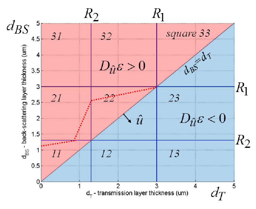
We will see later that the important regions, concerning the optimization process, are the regions square 11 (where $d_{BS}\leq R_{2}<R_{1}$ and $d_{T}\leq R_{2}<R_{1}$ ) and square 22 (where $R_{2}<d_{T}\leq R_{1}$ , $R_{2}<d_{BS}\leq R_{1}$ ).
In order to consider a non-orthogonal incidence of neutrons on the layers, it is sufficient to replace $\Sigma$ with $\frac{\Sigma}{\sin(\theta)}$ , where $\theta$ is the angle between the neutron beam and the layer surface (see Figure 1). This is valid for both the single blade case and for a multi-layer detector. The demonstration can be found in [11].

2.1 Monochromatic double layer optimization

In the domain region called square 11 the efficiency turns out to be:

\varepsilon_{11}\left(d_{BS},d_{T}\right)=A\cdot\left(1-e^{-\Sigma d_{BS}}\right)+d_{BS}\cdot C\cdot e^{-\Sigma d_{BS}}+e^{-\Sigma d_{BS}}\left(B\cdot\left(1-e^{-\Sigma d_{T}}\right)-C\cdot d_{T}\right)

(2)

Where we have called:

A=\left(1-\frac{1}{2\Sigma R_{1}}-\frac{1}{2\Sigma R_{2}}\right),\quad B=\left(1+\frac{1}{2\Sigma R_{1}}+\frac{1}{2\Sigma R_{2}}\right),\quad C=\left(\frac{1}{2R_{1}}+\frac{1}{2R_{2}}\right),\quad\Sigma=n\cdot\sigma(\lambda)

(3)

where $n$ is the number density of the converter layer and $\sigma(\lambda)$ its neutron absorption cross-section.
By calculating $\nabla\varepsilon_{11}(d_{BS},d_{T})=0$ we obtain the result that $d_{BS}=d_{T}$ and

d_{BS}=d_{T}=-\frac{1}{\Sigma}\cdot\ln\left(\frac{C}{\Sigma B}\right)

(4)

We repeat the procedure for the square 22 in which the efficiency is:

\begin{array}[]{ll}\varepsilon_{22}\left(d_{BS},d_{T}\right)&=A+\frac{e^{-\Sigma R_{2}}}{2\Sigma R_{2}}-\frac{e^{-\Sigma d_{BS}}}{2}\cdot\left(1-\frac{1}{\Sigma R_{1}}-\frac{d_{BS}}{R_{1}}\right)+\\ &+e^{-\Sigma d_{BS}}\cdot\left(-B\cdot e^{-\Sigma d_{T}}+\frac{1}{2}\left(1+\frac{1}{\Sigma R_{1}}-\frac{d_{T}}{R_{1}}\right)+\frac{e^{-\Sigma\left(d_{T}-R_{2}\right)}}{2\Sigma R_{2}}\right)\end{array}

(5)

We obtain again $d_{BS}=d_{T}$ and

d_{BS}=d_{T}=-\frac{1}{\Sigma}\cdot\ln\left(\frac{R_{2}}{R_{1}}\left(\frac{1}{2R_{2}\Sigma B-e^{+\Sigma R_{2}}}\right)\right)

(6)

Naturally each result of Equations 4 and 6 is useful only if it gives a value that falls inside the region it has been calculated for.
The points defined by Equations 4 and 6 define a maximum of the efficiency function in the regions square 11 or square 22 because the Hessian matrix in those points has a positive determinant and $\frac{\partial^{2}\varepsilon}{\partial d_{BS}^{2}}$ is negative.

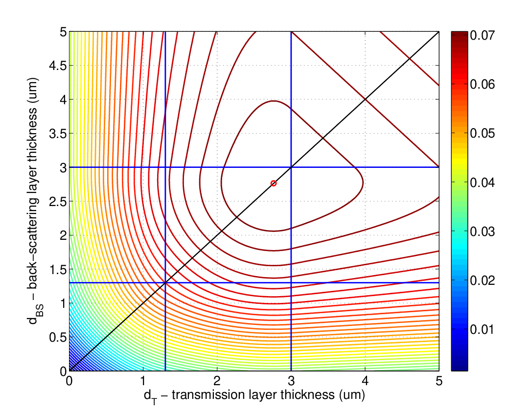
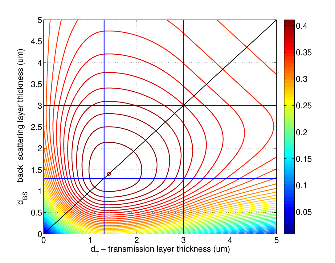
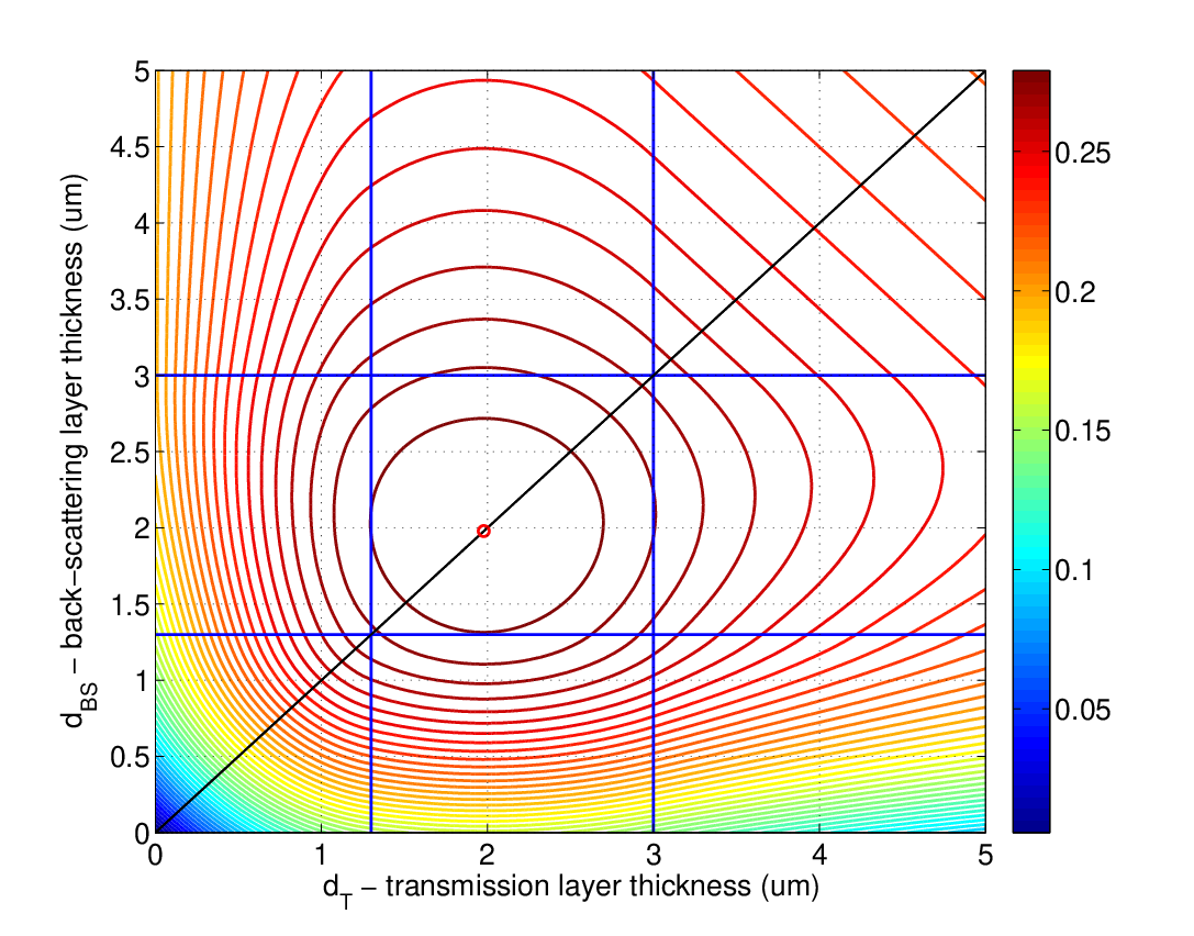
It is easy to demonstrate there are no extreme points outside the domain regions where either $d_{BS}>R_{1}$ or $d_{T}>R_{1}$ , i.e. square $jk$ with $j=3$ or $k=3$ or both. This outcome is also intuitive. In back-scattering mode when the converter thickness becomes thicker than the longest particle range ( $R_{1}$ ) there is no gain in efficiency by adding more converter material. In the transmission case, increasing the thickness above $R_{1}$ will add material that can only absorb neutrons without any particle escaping.
For the cases of squares 12 and 21, we obtain that $\nabla\varepsilon(d_{BS},d_{T})=0$ has no solution; thus the efficiency maximum can never fall in these domain regions.
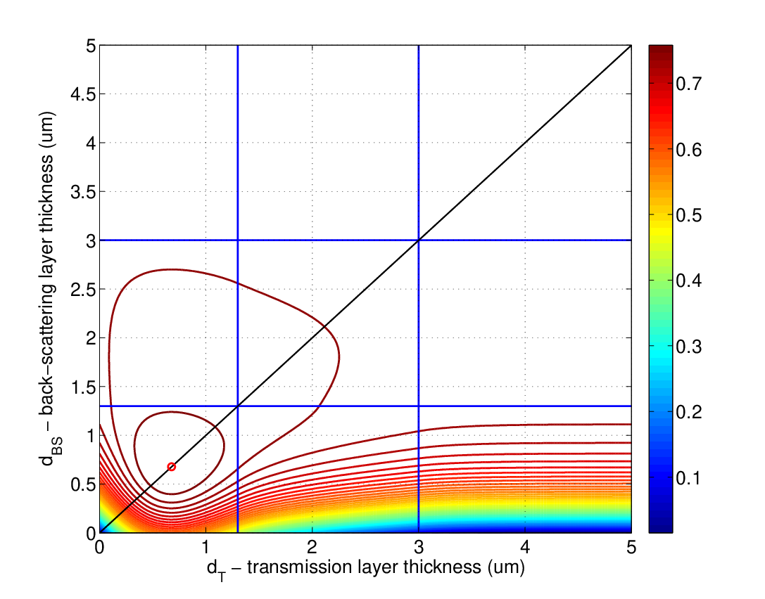
In Figures 3 and 4 the efficiency for four different cases is plotted. The red circle identifies the point of maximum efficiency calculated by using Equations 4 or 6; it stands out immediately that even though the efficiency function is not symmetric relatively to the domain bisector (drawn in black) the maximum nevertheless always lies on it.
This is a very important result because the sputtering deposition method [13] coats both sides of the substrate with the same thickness of converter material and it is also suited to make optimized blades.

2.2 Effect of the substrate

If we consider the neutron loss due to the substrate, the Equation 1 has to be modified as follows:

\varepsilon(d_{BS},d_{T})=\varepsilon_{BS}\left(d_{BS}\right)+\delta(\lambda)\cdot e^{-\Sigma\cdot d_{BS}}\cdot\varepsilon_{T}\left(d_{T}\right)

(7)

Where $\delta(\lambda)=e^{-\Sigma_{sub}(\lambda)\cdot d_{sub}}$ and $\Sigma_{sub}$ and $d_{sub}$ are the macroscopic cross-section and the thickness of the substrate.
If we optimize the layer thicknesses, we find the same result of Equations 4 and 6 for the transmission layer thickness $d_{T}$ but, on the other hand, the back-scattering layer thickness does not equal the transmission layer thickness anymore. It becomes:

d_{BS}=\begin{cases}\frac{1}{C}\cdot\left(1-\delta\right)+\delta\cdot d_{T}&\mbox{for \emph{square 11}}\\ R_{1}\cdot\left(1-2\delta\right)+\delta\cdot\left(1+\frac{R_{1}}{R_{2}}\right)\cdot d_{T}&\mbox{for \emph{square 21}}\\ R_{1}\cdot\left(1-\delta\right)+\delta\cdot d_{T}&\mbox{for \emph{square 22}}\end{cases}

(8)

The maximum efficiency can now also lie in square 21 but not in square 12, because $\delta\in[0,1]$ . The dotted line in squares 11, 21 and 22, in Figure 2, are Equations 8. The slope of the line in squares 11 and 22 is equal to $\delta(\lambda)<1$ . The maximum efficiency, when $\delta(\lambda)$ is not negligible, now lies on the dotted line just above the optimum without substrate effect.
From Equation 8 we can observe that when $\delta$ is close to zero, i.e. the substrate is very opaque to neutrons, the thickness of the back-scattering layer tends to the value $R_{1}$ . On the other hand, when $\delta$ is close to one, $d_{BS}$ tends to $d_{T}$ . The factor $\delta(\lambda)$ is usually very close to one for many materials that serve as substrate. We define the relative variation between $d_{BS}$ and $d_{T}$ as $\Delta_{d}=\left|\frac{d_{T}-d_{BS}}{d_{T}}\right|$ ; in Table 1 they are listed for a $0.5\,mm$ and $3\,mm$ Aluminium substrate of density $\rho=2.7\,g/cm^{3}$ at $1.8$ Å. In case the substrate is inclined under an angle of $10^{\circ}$ a substrate of $0.5\,mm$ looks like a substrate of about $3\,mm$ . We consider a neutron to be lost when it is either scattered or absorbed, therefore, the cross-section used [14] is: $\sigma_{Al}=\sigma_{Al}^{abs}(\lambda)+\sigma_{Al}^{scatt}=0.2\,b$ (at $1.8$ Å) $+1.5\,b=1.7\,b$ .

Table 1: Neutron loss factor

\delta

for an Aluminium substrate and relative difference between the two coating thicknesses held by the substrate for

1.8

Å.

$d_{sub}(mm)$	$\delta$ (1.8Å)	$\Delta_{d}$ (1.8Å)
0.5	0.995	0.0004
3	0.970	0.0026

2.3 Double layer for a distribution of neutron wavelengths

The result of having the same optimal coating thickness for each side of a blade is demonstrated for monochromatic neutrons and we want to prove it now for a more general case when the neutron beam is a distribution of wavelengths and when the substrate effect can be neglected ( $\delta(\lambda)\approx 1$ ).
We will prove a property that will turn out to be useful. We will show that the directional derivative of $\varepsilon(d_{BS},d_{T})$ along the unit vector $\hat{u}=\frac{1}{\sqrt{2}}\left(1,-1\right)$ is positive until the bisector $d_{BS}=d_{T}$ and it changes sign only there. This vector identifies the orthogonal direction to the bisector (see Figure 2).
In the square 11:

D_{\hat{u}}\varepsilon=\hat{u}\times\nabla\varepsilon(d_{BS},d_{T})=\frac{C\Sigma}{\sqrt{2}}\cdot e^{-\Sigma d_{BS}}\left(d_{BS}-d_{T}\right)

(9)

In the square 22:

D_{\hat{u}}\varepsilon=\frac{\Sigma}{2\sqrt{2}R_{1}}\cdot e^{-\Sigma d_{BS}}\left(d_{BS}-d_{T}\right)

(10)

Which are both positive above the bisector and negative below. In the other domain regions the demonstration is equivalent. E.g. in the square 12:

D_{\hat{u}}\varepsilon=-\frac{\Sigma}{2\sqrt{2}}\cdot e^{-\Sigma d_{BS}}\left(1-\frac{d_{BS}}{R_{2}}-\frac{d_{BS}}{R_{1}}+\frac{d_{T}}{R_{1}}\right)

(11)

Which is strictly negative in the square 12 where $d_{BS}\leq R_{2}<R_{1}$ and $R_{2}<d_{T}\leq R_{1}$ except in the corner, on the bisector, where $d_{BS}=d_{T}=R_{2}$ .
The following theorem is therefore proved.

Theorem 2.1

The efficiency function defined by the Equation 1 is strictly monotone in the two half-domains identified by the bisector $d_{BS}=d_{T}$ (see Figure 2).

In a general instrument design one can be interested in having a detector response for a whole range of $\lambda$ . E.g. an elastic instrument can work a certain time at one wavelength and another time at another wavelength. In a Time-Of-Flight instrument one can be interested in having a sensitivity to neutrons of a certain energy range including or excluding the elastic peak. One can define a normalized weight function $w\left(\lambda\right)$ ( $\int_{0}^{+\infty}w\left(\lambda\right)\,d\lambda=1$ ) that signifies how much that neutron wavelength is important compared to others. I.e. the price we want to spend in a neutron scattering instrument to be able to detect a neutron energy with respect to an other one. We can also consider an incident beam of neutrons, whose wavelength distribution is $w\left(\lambda\right)$ , and we want to maximize the efficiency given this distribution.
The efficiency for a blade exposed to a neutron flux which shows this distribution is:

\varepsilon_{w}(d_{BS},d_{T})=\int_{0}^{+\infty}w\left(\lambda\right)\varepsilon(d_{BS},d_{T},\lambda)\,d\lambda

(12)

where $\varepsilon(d_{BS},d_{T},\lambda)$ is the efficiency in Equation 1.
In order to optimize this efficiency its gradient relative to $d_{BS}$ and $d_{T}$ has to be calculated:

\nabla\varepsilon_{w}(d_{BS},d_{T})=\int_{0}^{+\infty}w\left(\lambda\right)\nabla\varepsilon(d_{BS},d_{T},\lambda)\,d\lambda

(13)

Both gradient components have to cancel out ( $\frac{\partial\varepsilon_{w}}{\partial d_{BS}}=\frac{\partial\varepsilon_{w}}{\partial d_{T}}=0$ ), this leads to $D_{\hat{u}}\varepsilon_{w}=0$ . E.g. in square 11: $\int_{0}^{+\infty}w\left(\lambda\right)\left(e^{-\Sigma d_{BS}}\left(d_{T}-d_{BS}\right)C\Sigma\right)\,d\lambda=0$ . As a result, in order for the efficiency to attain a maximum, it is necessary (but not sufficient) that its directional derivative along the unity vector $\hat{u}=\frac{1}{\sqrt{2}}\left(1,-1\right)$ :

D_{\hat{u}}\varepsilon_{w}=\int_{0}^{+\infty}w\left(\lambda\right)D_{\hat{u}}\varepsilon(d_{BS},d_{T},\lambda)\,d\lambda

(14)

equals zero.
For a general family of functions $f(d_{BS},d_{T},\lambda)$ for which the maximum always lies on the domain bisector it is not true that the function defined by their positively weighted linear combination must have the maximum on $d_{BS}=d_{T}$ , because in general $\nabla f(d_{BS},d_{T},\lambda)$ can be positive, null or negative, thus there are many ways to accomplish $\nabla f_{w}(d_{BS},d_{T})=0$ . However, thanks to Theorem 2.1, $D_{\hat{u}}\varepsilon=0$ is satisfied only on the bisector. Below the bisector, this is always negative, as it is a positively weighted integral of negative values; similarly, above the bisector, this is always positive. Hence, the maximum can only be attained on the bisector.
The gradient can hence be replaced by $\frac{\partial}{\partial d_{T}}$ and the function maximum has to be searched on the bisector, therefore:

\nabla\varepsilon_{w}(d_{T})=\int_{0}^{+\infty}w\left(\lambda\right)\frac{\partial}{\partial d_{T}}\varepsilon(d_{BS}=d_{T},d_{T},\lambda)\,d\lambda

(15)

In the end, the same layer thickness for both sides of a blade has to be chosen in order to maximize its efficiency, even if it is exposed to neutrons belonging to a general wavelength distribution $w\left(\lambda\right)$ .
The integration over $\lambda$ can be alternatively executed in the variable $\Sigma$ ; indeed $\Sigma$ is just a linear function in $\lambda$ because $\sigma_{abs}$ is proportional to $\lambda$ in the thermal neutron region. Moreover, as indicated previously, $\Sigma$ is also a function of $\theta$ and this is the only appearance of $\theta$ in the efficiency function. Hence, we can just as well consider a weighting in $\lambda$ and $\theta$ which results in just a weighting function over $\Sigma$ . In other words, all the results that have been derived for a wavelength distribution also hold for an angular distribution or both.

2.3.1 Flat neutron wavelength distribution example

As a simple example we take a flat distribution between two wavelengths $\lambda_{1}$ and $\lambda_{2}$ defined as follows:

w\left(\lambda\right)=\frac{1}{\lambda_{2}-\lambda_{1}}

(16)

In the square 11 we obtain:

\frac{\partial}{\partial d_{T}}\varepsilon(d_{BS}=d_{T},d_{T},\lambda)=2e^{-\Sigma d_{T}}\left(B\Sigma e^{-\Sigma d_{T}}-C\right)

(17)

We call $\Sigma_{1}=\Sigma(\lambda_{1})$ and $\Sigma_{2}=\Sigma(\lambda_{2})$ . We recall that A and B are function of $\Sigma(\lambda)$ .

\nabla\varepsilon_{w}(d_{T})=\frac{1}{(\Sigma_{2}-\Sigma_{1})}\left[\frac{e^{-2\Sigma d_{T}}}{d_{T}}\cdot\left(2Ce^{+\Sigma d_{T}}-C-\Sigma-\frac{1}{2d_{T}}\right)\right]_{\Sigma_{1}}^{\Sigma_{2}}=0

(18)

In the same way the solution in the square 22 can be determined.

\frac{\partial\varepsilon}{\partial d_{T}}=e^{-\Sigma d_{T}}\left(e^{-\Sigma d_{T}}\left(2B\Sigma-\frac{e^{+\Sigma R_{2}}}{R_{2}}\right)-\frac{1}{R_{1}}\right)

(19)

By integrating we finally obtain:

\nabla\varepsilon_{w}(d_{T})=\frac{1}{(\Sigma_{2}-\Sigma_{1})}\left[\frac{e^{-2\Sigma d_{T}}}{d_{T}}\left(\frac{e^{+\Sigma d_{T}}}{R_{1}}-C-\Sigma-\frac{1}{2d_{T}}-\frac{d_{T}\,e^{+\Sigma R_{2}}}{R_{2}\left(R_{2}-2d_{T}\right)}\right)\right]_{\Sigma_{1}}^{\Sigma_{2}}=0

(20)

The solution of Equations 18 and 20 gives the optimum value for the thickness of the two converter layers in the region of the domain called square 11 and square 22 respectively for a uniform neutron wavelength distribution between $\lambda_{1}$ and $\lambda_{2}$ . E.g. for a uniform neutron wavelength distribution between $1$ Å and $20$ Å the optimal thickness of coatings on both sides of the blade is $1\,\mu m$ .

3 The multi-layer detector design

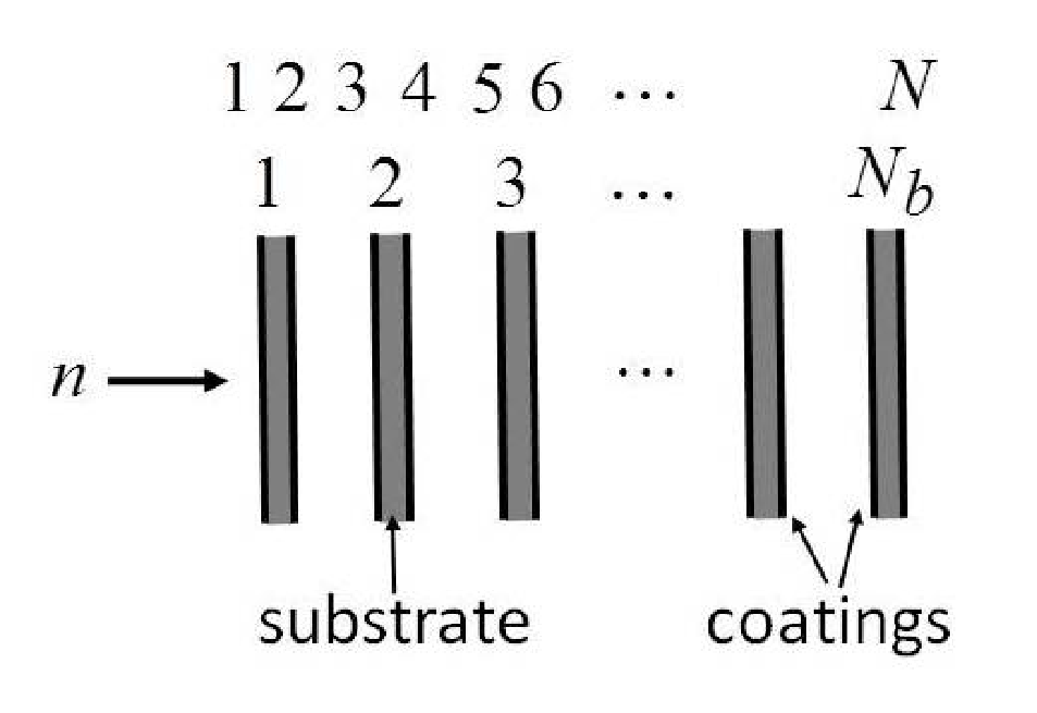
In a detector like that presented in [1], [15], or in [16], all the substrates have the same coating thickness. One can ask if it is possible to optimize the coating thicknesses for each layer in order to gain in efficiency. This is also applicable to neutron detectors which use solid converters coupled with GEMs [17]. In a multi-layer detector (see Figure 5), composed by $N$ layers or $N_{b}=\frac{N}{2}$ blades, the efficiency can be written as follows:

\varepsilon_{tot}(N_{b})=\varepsilon_{1}(d_{BS1},d_{T1})+\sum_{k=2}^{N_{b}}\varepsilon_{1}(d_{BSk},d_{Tk})\cdot e^{-\left(\sum_{j=1}^{\left(k-1\right)}\left(d_{BSj}+d_{Tj}\right)\right)\cdot\Sigma}

(21)

Where $\varepsilon_{1}(d_{BSk},d_{Tk})=\varepsilon_{1k}$ represents the efficiency for a single blade already defined by the Equation 1; $d_{BSk}$ and $d_{Tk}$ are the coating thicknesses of the $k-th$ blade.
If the detector is assembled with blades of the same thickness, i.e. $d_{BSk}=d_{Tk}=d,\,\,\forall k=1,2,\dots,N_{b}$ , Equation 21 can be simplified as follows:

\varepsilon_{tot}(N_{b})=\varepsilon_{1}(d)\cdot\sum_{k=1}^{N_{b}}e^{-2\left(k-1\right)d\cdot\Sigma}=\varepsilon_{1}(d)\cdot\frac{1-e^{-2d\Sigma N_{b}}}{1-e^{-2d\Sigma}}

(22)

Therefore, $\frac{d\varepsilon_{tot}}{dd}=0$ has to be calculated in order to optimize such a detector containing blades of same coating thicknesses.
In the case of a distribution of wavelengths, defined by $w\left(\lambda\right)$ , Equation 21 has to be integrated over $\lambda$ as already shown in Section 2.3.

\varepsilon_{tot}^{w}(N_{b},\bar{d}_{BS},\bar{d}_{T})=\int_{0}^{+\infty}w\left(\lambda\right)\varepsilon_{tot}(N_{b},\lambda)\,d\lambda

(23)

The efficiency will be function of $N=2\cdot N_{b}$ variables; which can be denoted using the compact vectorial notation by the two vectors $\bar{d}_{BS}$ and $\bar{d}_{T}$ of $N_{b}$ components each.
Both for monochromatic mode and for a distribution the detector optimization implies the calculation of the $N$ -dimensional gradient $\nabla\varepsilon_{tot}$ , because in the case of a distribution the gradient can be carried inside the integral over $\lambda$ . We will use the shorthand $\varepsilon_{1k}=\varepsilon_{1}\left(d_{BSk},d_{Tk}\right)$ .
The $k-th$ $N$ -dimensional gradient component for back-scattering mode results to be:

\frac{\partial\varepsilon_{tot}}{\partial d_{BSk}}=\begin{cases}\frac{\partial\varepsilon_{1k}}{\partial d_{BSk}}-\Sigma\cdot\sum_{p=\left(k+1\right)}^{N_{b}}\varepsilon_{1p}\cdot e^{-\left(\sum_{i=1}^{\left(p-1\right)}\left(d_{BSi}+d_{Ti}\right)\right)\cdot\Sigma}&\mbox{if \,}k=1\\ \frac{\partial\varepsilon_{1k}}{\partial d_{BSk}}\cdot e^{-\left(\sum_{j=1}^{\left(N_{b}-1\right)}\left(d_{BSj}+d_{Tj}\right)\right)\cdot\Sigma}-\Sigma\cdot\sum_{p=\left(k+1\right)}^{N_{b}}\varepsilon_{1p}\cdot e^{-\left(\sum_{i=1}^{\left(p-1\right)}\left(d_{BSi}+d_{Ti}\right)\right)\cdot\Sigma}&\mbox{if \, }1<k<N_{b}\\ \frac{\partial\varepsilon_{1k}}{\partial d_{BSk}}\cdot e^{-\left(\sum_{j=1}^{\left(N_{b}-1\right)}\left(d_{BSj}+d_{Tj}\right)\right)\cdot\Sigma}&\mbox{if \, }k=N_{b}\end{cases}

(24)

Equivalently we find the same formal expression for the $k-th$ component of the gradient with respect to the transmission variable ( $d_{T}$ ); we can substitute $\partial d_{BSk}$ with $\partial d_{Tk}$ in Equation 24 which are for the rest entirely the same. This implies that if we put identical conditions on $\frac{\partial\varepsilon_{tot}}{\partial d_{BSk}}$ and on $\frac{\partial\varepsilon_{tot}}{\partial d_{Tk}}$ this will result in $\frac{\partial\varepsilon_{1k}}{\partial d_{BS}}=\frac{\partial\varepsilon_{1k}}{\partial d_{T}}$ . Equivalently as already found in Section 2.3, from Equation 24 and the one for the transmission variable we finally obtain ( $\forall k=1,2,\dots,N_{b}$ ):

\begin{cases}\frac{\partial\varepsilon_{1k}}{\partial d_{BSk}}=\frac{\partial\varepsilon_{1k}}{\partial d_{Tk}}\Rightarrow D_{\hat{u}}\varepsilon_{1k}=0&\mbox{if \,}k<N_{b}\\ \frac{\partial\varepsilon_{1k}}{\partial d_{BSk}}=\frac{\partial\varepsilon_{1k}}{\partial d_{Tk}}=0&\mbox{if \, }k=N_{b}\end{cases}

(25)

Both for the monochromatic case and in the case of a distribution of wavelengths, the condition in Equation 25 has to be satisfied. Using Theorem 2.1, the maximum efficiency can only be found, again, on the bisector.
In a multi-layer detector, which has to be optimized for any distribution of neutron wavelengths or for a single wavelength, all the blades have to hold two layers of the same thickness. Naturally, thicknesses of different blades can be distinct.
Thanks to this property, we can denote with $d_{k}$ the common thickness of the two layers held by the $k-th$ blade ( $d_{BSk}=d_{Tk}=d_{k}$ ), furthermore, Equation 21 can be simplified as follows:

\varepsilon_{tot}(N,\bar{d})=\varepsilon_{1}(d_{1})+\sum_{k=2}^{N_{b}}\varepsilon_{1}(d_{k})\cdot e^{-2\left(\sum_{j=1}^{\left(k-1\right)}d_{j}\right)\cdot\Sigma}

(26)

where $\bar{d}$ is the vector of components $d_{k}$ for $k=1,2,\dots,N_{b}$ .
Optimizing a detector for a single neutron wavelength or for a distribution is different; the equation $\nabla\varepsilon_{tot}=0$ in one case and $\nabla\varepsilon_{tot}^{w}=0$ in the other represent a $N_{b}$ -dimensional system of equations in $N_{b}$ unknowns because of the simplification of having the same back-scattering and transmission layer thickness on the blades. By expanding the Equation 26 we obtain:

$\displaystyle\varepsilon_{tot}(N_{b})$	$\displaystyle=\varepsilon_{1}(d_{1})+e^{-2d_{1}\Sigma}\cdot\varepsilon_{1}(d_{2})+e^{-2d_{1}\Sigma}\cdot e^{-2d_{2}\Sigma}\cdot\varepsilon_{1}(d_{3})+\dots$	(27)
	$\displaystyle\dots+e^{-2d_{1}\Sigma}\cdot\dots\cdot e^{-2d_{BS(N_{b}-1)}\Sigma}\cdot\varepsilon_{1}(d_{N_{b}})=$
	$\displaystyle=\varepsilon_{1}(d_{1})+e^{-2d_{1}\Sigma}\cdot\left[\varepsilon_{1}(d_{2})+e^{-2d_{2}\Sigma}\cdot\left[\dots\left[\varepsilon_{1}(d_{(N_{b}-1)})+e^{-2d_{(N_{b}-1)}\Sigma}\cdot\varepsilon_{1}(d_{N_{b}})\right]\dots\right]\right]$

We notice that the variable $d_{N_{b}}$ appears only once, this means that, in the case of a single wavelength, its value can be determined without taking the others into account. Continuing the reasoning we see that the system of equations is upper triangular. In the monochromatic case we can optimize the detector starting from the last blade and going backward till the first. This is not true for the distribution case in which the gradient of Equation 27 is in addition integrated over $\lambda$ , thus all the blades have to be taken into account simultaneously in the optimization process. In the monochromatic case, we can start by fixing the last blade coating thickness because any change on the previous will only affect the number of neutrons that reach the last blade, and we require the last blade to be as efficient as possible for that kind of neutron. As the layer thickness optimum of each blade does not depend on the previous ones, the system is triangular. On the other hand, in the case of a wavelength distribution, any change on the previous blades will change the actual distribution of wavelengths the last blade experiences. Thus, the neutron distribution a blade has to be optimized for depends on all the previous blade coatings. In this case, the system is not triangular.

3.1 Monochromatic multi-layer detector optimization

In order to optimize the layers in multi-layer detectors for a given neutron wavelength, we can maximize the last layer efficiency and, then, go backward until the first layer. Formally, from Equation 27, we obtain an iterative structure:

f_{k}=\begin{cases}\varepsilon_{1}(d_{k})+e^{-2d_{k}\Sigma}\cdot\alpha_{k+1}&\mbox{if \,}k<N_{b}\\ \varepsilon_{1}(d_{k})&\mbox{if \, }k=N_{b}\end{cases}

(28)

$\alpha_{k+1}$ is a fixed number, independent from $d_{k}$ , and represents the cumulative efficiency of the detector from the blade $(k+1)-th$ to the end.

\frac{df_{k}}{dd_{k}}=\begin{cases}\frac{d}{dd_{k}}\varepsilon_{1}(d_{k})-2\Sigma\,e^{-2d_{k}\Sigma}\cdot\alpha_{k+1}&\mbox{if \,}k<N_{b}\\ \frac{d}{dd_{k}}\varepsilon_{1}(d_{k})&\mbox{if \, }k=N_{b}\end{cases}

(29)

$\frac{d}{dd_{k}}\varepsilon_{1}(d_{k})$ are the derivatives in Equations 17 and 19 according to the domain partitions. In the domain region called square 11 as defined in Section 2, we obtain:

\frac{df_{k}}{dd_{k}}=\begin{cases}2e^{-\Sigma d_{k}}\left(\left(B-\alpha_{k+1}\right)\Sigma e^{-\Sigma d_{k}}-C\right)&\mbox{if \,}k<N_{b}\\ 2e^{-\Sigma d_{k}}\left(B\Sigma e^{-\Sigma d_{k}}-C\right)&\mbox{if \, }k=N_{b}\end{cases}

(30)

And in the square 22:

\frac{df_{k}}{dd_{k}}=\begin{cases}e^{-\Sigma d_{k}}\left(e^{-\Sigma d_{k}}\left(2\left(B-\alpha_{k+1}\right)\Sigma-\frac{e^{+\Sigma R_{2}}}{R_{2}}\right)-\frac{1}{R_{1}}\right)&\mbox{if \,}k<N_{b}\\ e^{-\Sigma d_{k}}\left(e^{-\Sigma d_{k}}\left(2B\Sigma-\frac{e^{+\Sigma R_{2}}}{R_{2}}\right)-\frac{1}{R_{1}}\right)&\mbox{if \, }k=N_{b}\end{cases}

(31)

Equations 30 and 31 have solutions similar to 4 and 6. In the square 11 the solution is:

d_{k}^{opt}=\begin{cases}-\frac{1}{\Sigma}\cdot\ln\left(\frac{C}{\left(B-\alpha_{k+1}\right)\Sigma}\right)&\mbox{if \,}k<N_{b}\\ -\frac{1}{\Sigma}\cdot\ln\left(\frac{C}{B\Sigma}\right)&\mbox{if \, }k=N_{b}\end{cases}

(32)

In the square 22:

d_{k}^{opt}=\begin{cases}-\frac{1}{\Sigma}\cdot\ln\left(\frac{R_{2}}{R_{1}}\left(\frac{1}{2R_{2}\Sigma\left(B-\alpha_{k+1}\right)-e^{+\Sigma R_{2}}}\right)\right)&\mbox{if \,}k<N_{b}\\ -\frac{1}{\Sigma}\cdot\ln\left(\frac{R_{2}}{R_{1}}\left(\frac{1}{2R_{2}\Sigma B-e^{+\Sigma R_{2}}}\right)\right)&\mbox{if \, }k=N_{b}\end{cases}

(33)

The optimization method is a recursive procedure that employs the Equations 32 and 33; we start from the last blade, and we find its optimal thickness $d_{N_{b}}^{opt}$ , afterwards we calculate $\alpha_{N_{b}}$ as the last layer efficiency using the optimal thickness found. Now we can calculate $d_{N_{b}-1}^{opt}$ from Equations 32 or 33 and $\alpha_{N_{b}-1}$ and so on until the first layer.

\alpha_{k+1}=\begin{cases}\varepsilon_{1}(d_{k+1}^{opt})+\sum_{i=k+2}^{N_{b}}\varepsilon_{1}(d_{i}^{opt})\cdot e^{-2\left(\sum_{j=k+1}^{\left(i-1\right)}d_{j}^{opt}\right)\cdot\Sigma}&\mbox{if \,}k+1<N_{b}\\ \varepsilon_{1}(d_{k+1}^{opt})&\mbox{if \, }k+1=N_{b}\end{cases}

(34)

3.1.1 Example of application

We analyze a detector composed of $30$ successive converter layers ( $15$ blades) crossed by the neutron beam at $90^{\circ}$ (like in Figure 5). We consider ${}^{10}B_{4}C$ ( $\rho=2.24\,g/cm^{3}$ ) as converter; we neglect again the $6\%$ branching ratio of ${}^{10}B$ neutron capture reaction. A $100\,KeV$ energy threshold is applied and particle ranges turn out to be $R_{1}=3\,\mu m$ ( $\alpha$ -particle) and $R_{2}=1.3\,\mu m$ ( ${}^{7}Li$ ), for the $94\%$ branching ratio.
Figures 6 and 7 show the optimization result for this multi-layer detector; for a monochromatic neutron beam of $1.8$ Å and $10$ Å. On the left, the optimal thickness given by either Equations 32 or 33 is plotted in red for each blade; for comparison we use two similar detectors suitable for short and for long wavelengths in which the blades are holding $1.2\,\mu m$ and $0.5\,\mu m$ thickness coating. Those values have been obtained by optimizing the Equation 22, the efficiency for a detector holding $15$ blades of all equal thicknesses for $1.8$ Å and for for $10$ Å. The detector with $1.2\,\mu m$ coatings is very close to the one presented in [1]. On the right, in Figures 6 and 7, the efficiency contribution of each blade is plotted, again for an optimized detector for $1.8$ Å and for an optimization done for $10$ Å. The expression of the efficiency as a function of the detector depth is given by Equation 26 for each blade by fixing the index $k$ .

Table 2: Efficiency for an optimized multi-layer detector and for a detector which contains

15

identical blades of

1.2\,\mu m

and

0.5\,\mu m

wavelength (Å)	opt. detect.	$0.5\,\mu m$ detect.	$1.2\,\mu m$ detect.
1.8	0.525	0.388	0.510
10	0.858	0.831	0.671

The whole detector efficiency is given in the end by summing all the blades’ contributions. The whole detector efficiency is displayed in Table 2 for the detector of Figures 6 and 7. By optimizing the detector for a given neutron wavelength we gain only about $2\%$ efficiency which is equivalent to add more layers to the detectors optimized to hold identical blades.
In Figure 8 is shown the efficiency resulting from the monochromatic optimization process of the individual blade coatings and the optimization for a detector containing all identical blades (which thicknesses are shown on the right for each neutron wavelength). Neutrons hit the layers at $90^{\circ}$ and five cases have been taken into account with an increasing number of layers. We notice that about for all neutron wavelengths the gain in optimizing the detector with different blades, let us to gain few percent in efficiency. The values in Table 2 are the values on the pink solid curve and the dashed one at $1.8$ Å and at $10$ Å in Figure 8.

Still referring to Figure 8, we notice that a detector with 15 individually optimized blades (30 layers) has about the same efficiency (above $10$ Å) than a detector optimized to contain 20 blades (40 layers) of equal thickness. On the other hand for short wavelengths the difference is not very significant. Moreover, there is also a trade off between the constraints of the detector construction and the complexity of the blade production.

3.2 Multi-layer detector optimization for a distribution of neutron wavelengths

In this case it is not possible to start the optimization from the last blade because the thicknesses of the previous layers will affect the neutron wavelength distribution reaching the deeper laying blades. We have in this case to optimize an $N_{b}$ -dimensional function at once. Therefore, the $N_{b}$ -dimensional equation $\nabla\varepsilon_{tot}^{w}=0$ has to be solved:

\nabla_{k}\varepsilon_{tot}^{w}=\int_{0}^{+\infty}w\left(\lambda\right)\frac{\partial\varepsilon_{tot}}{\partial d_{k}}\,d\lambda=0

(35)

$\frac{\partial\varepsilon_{tot}}{\partial d_{k}}$ is an expression similar to Equation 24 provided that we impose $d_{BSk}=d_{Tk}\,\forall k=1,2,\dots,N_{b}$ .
In order to optimize a detector for a given neutron wavelength distribution $w\left(\lambda\right)$ , the following system of $N_{b}$ equations in $N_{b}$ unknown ( $d_{k}$ ) has to be solved:

\begin{cases}\int_{0}^{+\infty}w\left(\lambda\right)\left[\frac{\partial\varepsilon_{1}(d_{k})}{\partial d_{k}}-2\Sigma\cdot\sum_{p=\left(k+1\right)}^{N_{b}}\varepsilon_{1}(d_{p})\cdot e^{-2\left(\sum_{i=1}^{\left(p-1\right)}d_{i}\right)\cdot\Sigma}\right]\,d\lambda=0&\mbox{if \,}k=1\\ \int_{0}^{+\infty}w\left(\lambda\right)\left[\frac{\partial\varepsilon_{1}(d_{k})}{\partial d_{k}}\cdot e^{-2\left(\sum_{j=1}^{\left(N_{b}-1\right)}d_{j}\right)\cdot\Sigma}\right.+\\ -\left.2\Sigma\cdot\sum_{p=\left(k+1\right)}^{N_{b}}\varepsilon_{1}(d_{p})\cdot e^{-2\left(\sum_{i=1}^{\left(p-1\right)}d_{i}\right)\cdot\Sigma}\right]\,d\lambda=0&\mbox{if \, }1<k<N_{b}\\ \int_{0}^{+\infty}w\left(\lambda\right)\left[\frac{\partial\varepsilon_{1}(d_{k})}{\partial d_{k}}\cdot e^{-2\left(\sum_{j=1}^{\left(N_{b}-1\right)}d_{j}\right)\cdot\Sigma}\right]\,d\lambda=0&\mbox{if \, }k=N_{b}\end{cases}

(36)

We recall that $\varepsilon_{1}(d_{k})$ and $\Sigma$ are function of $\lambda$ and $\varepsilon_{1}(d_{k})$ is the blade efficiency defined in Equations 2 and 5; its derivative $\frac{\partial\varepsilon_{1}(d_{k})}{\partial d_{k}}$ was already calculated in the Equations 17 and 19 (Section 2).
The system of equations 36 can easily be solved numerically.

3.2.1 Flat neutron wavelength distribution example

We take a flat distribution $w\left(\lambda\right)=\frac{1}{\lambda_{2}-\lambda_{1}}$ between the two wavelengths $\lambda_{1}=1$ Å and $\lambda_{2}=20$ Å as in Section 2 for the single blade case. In Figure 9 the thicknesses of each of the blade coatings and each blade efficiency contribution for a $30$ -layer detector are shown. Three detectors are compared, the one of simplest construction is a detector holding $15$ identical blades of $0.5\,\mu m$ coating thickness, the second is a detector optimized according to Equation 36 for that specific flat distribution and the last is a detector that has been optimized for a single neutron wavelength of $10$ Å conforming to Equations 32, 33 and 34. The fact to have a contribution of wavelengths shorter than $10$ Å in the case of the red line makes the coating thicknesses larger compared to the blue curve.
As a result, frontal layers are slightly more efficient for the optimized detector than for the one optimized for $10$ Å; on the other hand, deep layers lose efficiency.

Figure 10 shows the three detector efficiencies as a function of neutron wavelength. By comparing red and blue lines, of which the difference is plotted on the right plot, the optimized detector gains efficiency on shorter wavelengths but loses on longer. Moreover, we notice that the optimization process explained in this section let to gain at most $3.5\%$ at short wavelengths while losing less than $1\%$ on longer ones. The weighted efficiency over $w\left(\lambda\right)$ is shown in Table 3.

Table 3: Averaged efficiency over the flat neutron wavelength distribution (

1

Å-

20

Å) for a detector which contains

15

identical blades of

0.5\,\mu m

, for an optimized multi-layer detector for that specific flat distribution and for a detector optimized for

10

Å(Energy threshold of

100\,KeV

is applied).

opt. detect.	opt. detect. for 10Å	$0.5\,\mu m$ detect.
0.796	0.793	0.764

We can conclude that if we are interested in optimizing a detector in a given interval of wavelengths without any preference to any specific neutron energy; optimizing according to Equation 36 does not give a big improvement in the average efficiency compared to optimizing for the neutron wavelength distribution barycenter (about $10$ Å).
Although the averaged efficiency for the optimized detector in the neutron wavelength range differs from the one optimized for $10$ Å only by $0.3\%$ one can be interested to have a better efficiency for shorter wavelengths rather than for longer. It is in this case that the optimization process can play a significant role. On that purpose let’s move to the following example.

3.2.2 Hyperbolic neutron wavelength distribution example

We consider a hyperbolic neutron wavelength distribution between $\lambda_{1}=1$ Å and $\lambda_{2}=20$ Å.

w\left(\lambda\right)=\frac{1}{\ln\left(\frac{\lambda_{2}}{\lambda_{1}}\right)}\cdot\frac{1}{\lambda}

(37)

This optimization aims to give equal importance to bins on a logarithmic wavelength scale. The barycenter of the wavelength distribution corresponds to $\int_{\lambda_{1}}^{\lambda 2}w\left(\lambda\right)\lambda\,d\lambda=6.34$ Å.
In Figure 11 are shown the thicknesses of each blade coating and the efficiency as a function of the depth direction in the detector for a $30$ -layer detector. Five detectors are compared, the one of $1.2\,\mu m$ coating thickness, a detector optimized according to Equation 36 for that specific hyperbolic distribution, a detector that has been optimized for a single neutron wavelength of $10$ Å, $1.8$ Å, and for the barycenter of the distribution.

Table 4: Averaged efficiency over the hyperbolic distribution for a detector which contains

15

identical blades of

1.2\,\mu m

, for an optimized multi-layer detector for that specific distribution and for a detector optimized for

10

Å,

6.34

Å and for

1.8

Å (Energy threshold of

100\,KeV

applied).

opt. detect.	opt. $10$ Å	opt. $6.34$ Å	opt. $1.8$ Å	$1.2\,\mu m$ detect.
0.671	0.641	0.664	0.639	0.597

Figure 12 shows the five detector efficiencies as a function of wavelength and their difference on the right plot. By comparing the red (optimized detector) and the blue (detector optimized for $10$ Å) lines, of which the difference is plotted in blue on the right plot, we notice that the detector optimized for such a distribution gains about $9\%$ efficiency at short wavelengths and loses about $4\%$ at high wavelengths. A detector conceived for short wavelengths, such as the one represented by the pink line, has an opposite behavior instead. The distribution optimized detector gains efficiency for long wavelengths reaching about $11\%$ . Moreover, a detector optimized for the barycenter of the neutron wavelength distribution, instead does not differ more than about $4\%$ over the whole wavelength interval, as in the case of a uniform distribution. By only comparing the averaged efficiencies, shown in Table 4, it seems that there is not a big improvement in the detector efficiency which is only about $3\%$ for both $10$ Å and $1.8$ Å optimized detectors with respect to the distribution optimized detector. On the other hand, the optimization procedure, explained in this section, shows that it can lead to a significant efficiency improvement in certain neutron wavelength ranges. Furthermore, as in the case of a flat distribution, a detector optimized for a distribution according to Equations 36, does not show significant improvement in performances with respect to a detector just optimized for its barycenter.

4 Considerations on solid converter Pulse Height Spectra

The physical model taken into account in [11] and in [12] can be used as well to derive the analytical formula for the Pulse Height Spectra (PHS). A similar work was done in [12] (see Appendix B) where only Monte Carlo solutions were shown; here we want to use analytic methods to understand the structure of the PHS.
We make approximation mentioned in the introduction and we assume either a simplified stopping power function (see Section 4.1.2) or one simulated with SRIM [18] for the neutron capture fragments.
We calculate the probability for a particle emitted from the conversion point to travel exactly a distance $L$ on a straight line towards the escape surface (see Figure 1). This distance $L$ is related to the charged particle remaining energy through the primitive function of the stopping power. We will demonstrate that even under strong approximations of the stopping power function the model still predicts quite well the important physical features of the PHS.

4.1 Back-scattering mode

The probability for a neutron to be captured at depth $\left(x,x+dx\right)$ in the converter layer and for the capture reaction fragment (emitted isotropically in $4\pi\,sr$ ) to be emitted with an angle $\varphi=\arccos(u)$ (between $\left(u,u+du\right)$ ) is:

p(x,u)dx\,du=\begin{cases}\frac{1}{2}\cdot\Sigma e^{-\Sigma\cdot x}\,dx\,du&\mbox{if \,}x\leq d\\ 0&\mbox{if \, }x>d\end{cases}

(38)

Where $\Sigma$ is the macroscopic cross-section already defined in Equation 3 and $d$ is the layer thickness.
The fragment will travel a distance $L$ across the converter layer if $L=\frac{x}{u}$ and $u\in[0,1]$ .
The probability for a particle to travel a distance $\left(L,L+dL\right)$ across the layer is then given by:

P(L)\,dL=\int_{0}^{d}\,dx\int_{0}^{1}\,du\,\,\delta\left(\frac{x}{u}-L\right)p(x,u)=\begin{cases}\frac{1}{2L^{2}}\left(\frac{1}{\Sigma}-(\frac{1}{\Sigma}+L)e^{-\Sigma\cdot L}\right)\,dL&\mbox{if \,}L\leq d\\ \frac{1}{2L^{2}}\left(\frac{1}{\Sigma}-(\frac{1}{\Sigma}+d)e^{-\Sigma\cdot d}\right)\,dL&\mbox{if \, }L>d\end{cases}

(39)

It is sufficient to replace $\Sigma$ with $\frac{\Sigma}{\sin(\theta)}$ if neutrons hit the layer under the angle $\theta$ with respect to the surface (see Figure 1). The demonstration is equivalent to the one that can found in [11] for the efficiency function, in the PHS calculation $p(x,u)$ has to be changed as follows:

p(x,u,\theta)dx\,du=\begin{cases}\frac{1}{2}\cdot\Sigma e^{-\Sigma\cdot\frac{x}{\sin{(\theta)}}}\frac{dx}{\sin{(\theta)}}\,du&\mbox{if \,}x\leq d\\ 0&\mbox{if \, }x>d\end{cases}

(40)

If $E(L)$ is the remaining energy of a particle that has traveled a distance $L$ into the layer, $\frac{dE(L)}{dL}$ is the stopping power or equivalently the Jacobian of the coordinate transformation between $L$ and $E$ .
Once $P(L)dL$ is known we can calculate $Q(E)dE$ , therefore:

Q(E)dE=P(L(E))\cdot\frac{1}{\left|\frac{dE}{dL}\right|}\cdot dE

(41)

where $Q(E)dE$ is the probability that an incident neutron will give rise to a release of an energy $\left(E,E+dE\right)$ in the gas volume; hence it is the analytical expression for the PHS.

4.1.1 PHS calculation using SRIM output files for Stopping Power

We take the case of the ${}^{10}B$ reaction as example, however results can be applied to any solid neutron converter. We recall the energies carried for the $94\%$ branching ratio is $E_{0}=1470KeV$ for the $\alpha$ -particle and $E_{0}=830KeV$ for the ${}^{7}Li$ ; for the $6\%$ branching ratio, $E_{0}=1770KeV$ for the $\alpha$ -particle and $E_{0}=1010KeV$ for the ${}^{7}Li$ . Referring to Equation 41, the stopping power $\frac{dE}{dL}$ used here was simulated with SRIM [18] (see Figure 14) and $L(E)$ obtained by numerical inversion of the stopping power primitive function, i.e. the remaining energy inverse function.
The complete PHS can be obtained adding the four PHS in the case of ${}^{10}B$ according to the branching ratio probability:

Q_{tot}(E)dE=\left(0.94\cdot\left(Q_{\alpha}(E)+Q_{{}^{7}Li}(E)\right)\right.+0.06\cdot\left.\left(Q_{\alpha}(E)+Q_{{}^{7}Li}(E)\right)\right)\cdot dE

(42)

Consequently the efficiency for a single layer can be calculated by:

\varepsilon\left(E_{Th}\right)=\int_{E_{Th}}^{+\infty}Q_{tot}(E)dE

(43)

Where $E_{Th}$ is the energy threshold applied to cut the PHS. This result is fully in agreement with what can be calculated by using the Equations in [11].
A Multi-Grid-like detector [1] was used to collect the data at ILL-CT2 where a monochromatic neutron beam of $2.5$ Å is available. This particular detector has the peculiarity that in each of its frames blades of different coating thickness were mounted; as a result the simultaneous PHS measurement for different layer thicknesses has been possible. The blades are made up of an Aluminium substrate of $0.5\,mm$ thickness coated on both sides by an enriched ${}^{10}B_{4}C$ layer [13]. Thicknesses available in the detector were: $0.50\,\mu m$ , $0.75\,\mu m$ , $1\,\mu m$ , $1.5\,\mu m$ , $2\,\mu m$ and $2.5\,\mu m$ .
In our calculation we are not taking into account several processes, such as wall effects, gas amplification and fluctuations, space charge effects, etc. but only the neutron conversion and the fragment escape. Moreover, while the calculation has an infinite energy precision, this is not the case on a direct measurement because many processes give a finite energy resolution.
In order to be able to compare calculations and measurements, after the PHS were calculated for the thicknesses listed above, we convolve them with a gaussian filter of $\sigma=10\,KeV$ . The measured PHS were normalized to the maximum energy yield ( $1770\,KeV$ ). An energy threshold of $180\,KeV$ was applied to the calculation to cut the spectrum at low energies at the same level the measured PHS was collected.
We compare calculated and measured PHS in Figure 13; we can conclude that the model gives realistic results in sufficient agreement with the experimental ones, to be able to describe its main features.

4.1.2 PHS calculation using a strong approximation

A fully analytical result that does not appeal to experimental or SRIM-calculated stopping power functions, can be useful to understand the PHS structure and to determine its properties.
The stopping power functions $\frac{dE}{dL}$ can be approximated by a constant in the case of an $\alpha$ -particle and with a linear dependency in $L$ for a ${}^{7}Li$ -ion. As a result the energy dependency as a function of the traveled distance $L$ is given by:

E_{\alpha}(L)=\begin{cases}-\frac{E_{0}}{R}\left(L-R\right)&\mbox{if \,}L\leq R\\ 0&\mbox{if \, }L>R\end{cases}

(44)

And equivalently for the ${}^{7}Li$ -fragment:

E_{Li}(L)=\begin{cases}\frac{E_{0}}{R^{2}}\left(L-R\right)^{2}&\mbox{if \,}L\leq R\\ 0&\mbox{if \, }L>R\end{cases}

(45)

Where $R$ is the particle range and $E_{0}$ its initial energy.
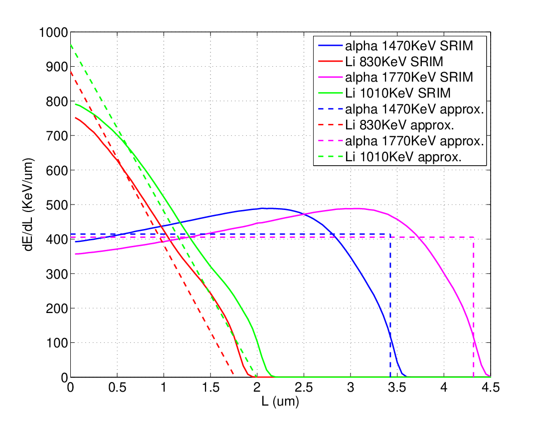
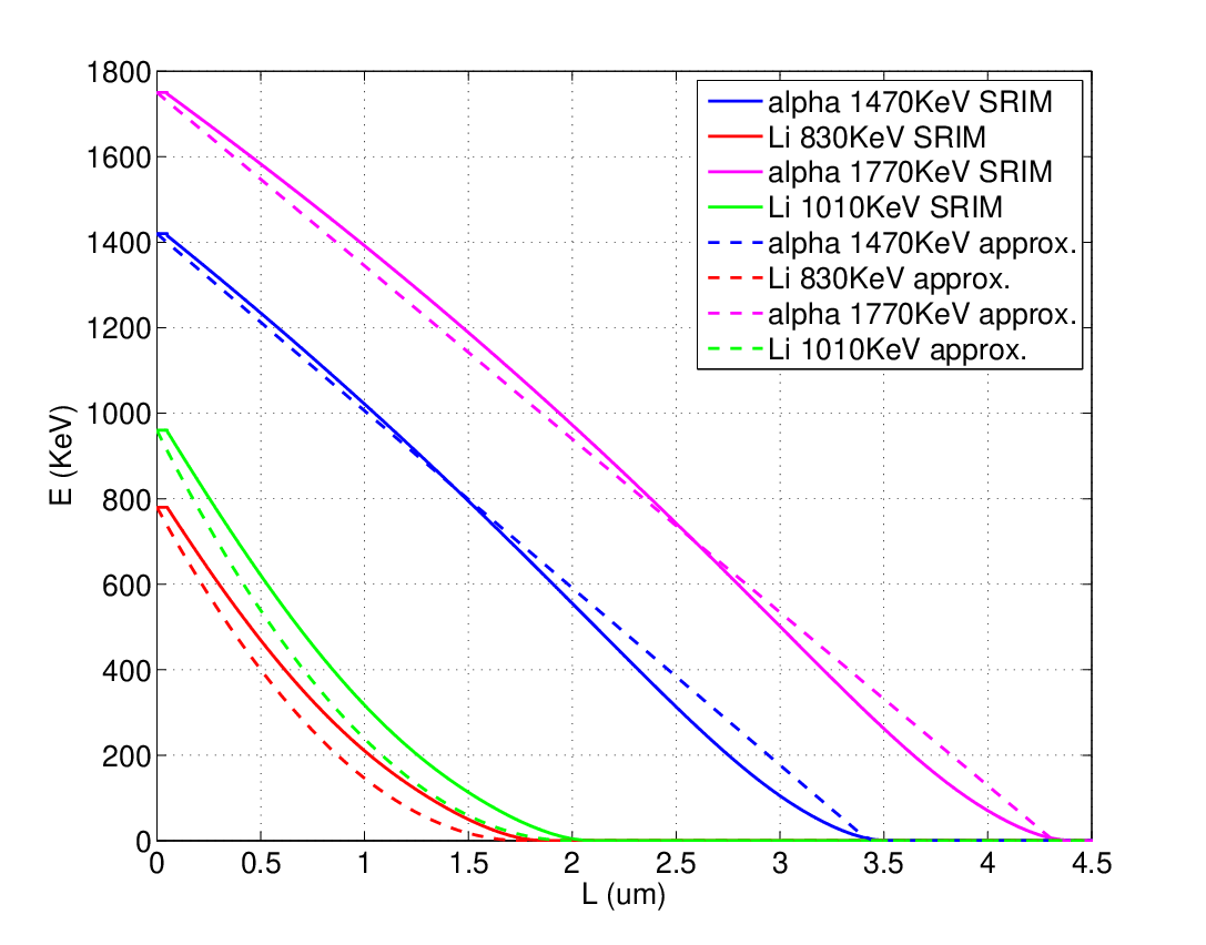
In Figure 14 are shown the stopping power functions $\frac{dE}{dL}$ for ${}^{10}B$ -reaction fragments and their integral $E(L)$ , in the case of using SRIM (solid lines) and in the case we use the expression displayed in the Equations 44 and 45 (dashed lines).

By substituting Expressions 44 and 45 into the Equation 41 we obtain a fully analytical formula for the PHS. It has to be pointed out that each relation, valid for $L\leq R$ , is valid in the range $E\leq E_{0}$ . Hence Equations 46 and 47 hold for $E\leq E_{0}$ . The two formulations in Equation 39 for $L\leq d$ and $L>d$ , translate in two different analytical expressions for $Q(E)$ for $E<E^{*}$ and for $E\geq E^{*}$ , with $d=L(E^{*})$ .
For the $\alpha$ -particle:

Q(E)\,dE=\begin{cases}\frac{1}{2E_{0}R\left(1-\frac{E}{E_{0}}\right)^{2}}\left(\frac{1}{\Sigma}-(\frac{1}{\Sigma}+d)e^{-\Sigma d}\right)\,dE&\mbox{if \,}E<E_{0}\left(1-\frac{d}{R}\right)\\ \frac{1}{2E_{0}R\left(1-\frac{E}{E_{0}}\right)^{2}}\left(\frac{1}{\Sigma}-\left(\frac{1}{\Sigma}+R\left(1-\frac{E}{E_{0}}\right)\right)\cdot e^{-\Sigma R\left(1-\frac{E}{E_{0}}\right)}\right)\,dE&\mbox{if \, }E\geq E_{0}\left(1-\frac{d}{R}\right)\end{cases}

(46)

Where the relation $E^{*}=E_{0}\left(1-\frac{d}{R}\right)$ is derived from $d=L(E^{*})$ .
For the ${}^{7}Li$ :

Q(E)\,dE=\begin{cases}\frac{1}{4E_{0}R\sqrt{\frac{E}{E_{0}}}\left(1-\sqrt{\frac{E}{E_{0}}}\right)^{2}}\left(\frac{1}{\Sigma}-(\frac{1}{\Sigma}+d)e^{-\Sigma\cdot d}\right)\,dE&\mbox{if \,}E<E_{0}\left(1-\frac{d}{R}\right)^{2}\\ \frac{1}{4E_{0}R\sqrt{\frac{E}{E_{0}}}\left(1-\sqrt{\frac{E}{E_{0}}}\right)^{2}}\left(\frac{1}{\Sigma}-\left(\frac{1}{\Sigma}+\right.\right.\\ +\left.\left.R\left(1-\sqrt{\frac{E}{E_{0}}}\right)\right)\cdot e^{-\Sigma R\left(1-\sqrt{\frac{E}{E_{0}}}\right)}\right)\,dE&\mbox{if \, }E\geq E_{0}\left(1-\frac{d}{R}\right)^{2}\end{cases}

(47)

Where, again, the relation $E^{*}=E_{0}\left(1-\frac{d}{R}\right)^{2}$ is derived from the condition $d=L(E^{*})$ .
Figures 15, 16 and 17 show the calculated PHS obtained by using the SRIM stopping power functions and the approximated one displayed in the Expression 44 and 45 for $0.2\,\mu m$ , $1\,\mu m$ and $4\,\mu m$ respectively, when neutrons hit at $90^{\circ}$ the surface and their wavelength is $1.8$ Å. They show similar shapes that differ in some points; e.g. focusing on the $1470\,KeV$ $\alpha$ -particle, the fact that the approximated $E(L)$ function (see Figure 14) differs from the SRIM one at high $L$ leads to a disappearance of the PHS rise at low energies; it is clearly visible in Figure 17.
We see that as $d$ increases what looked like a single peak splits into two peaks. While one peak stays constant at the highest fragment energy $E_{0}$ the second one moves toward lower energies when the layer thickness increases. This is important when trying to improve the neutron to gamma-rays discrimination by creating a valley that separates them in amplitude.

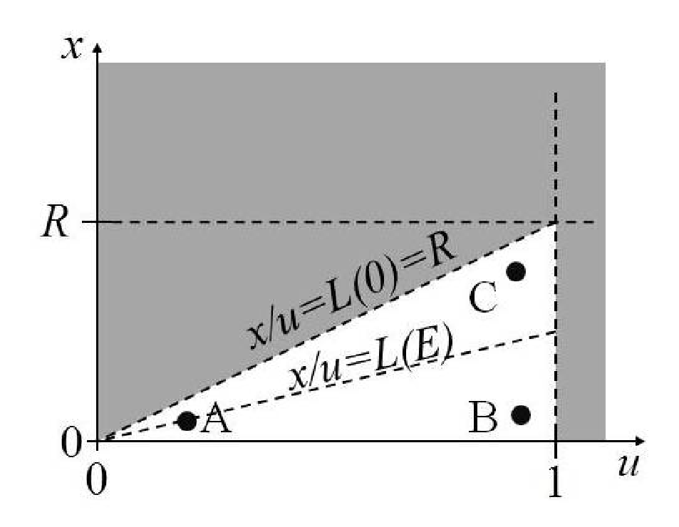
In order to understand the PHS structure, we define the PHS variable space: on the abscissa axis is plotted $u=\cos(\varphi)$ , where $\varphi$ is the angle the fragment has been emitted with, and, on the ordinates axis, is plotted the neutron absorption depth $x$ . $u\in\left[0,1\right]$ ; $x\in\left[0,d\right]$ if $d<R$ or $x\in\left[0,R\right]$ if $d\geq R$ because a neutron can only be converted inside the layer and, on the other hand, if a neutron is converted too deep into the layer, i.e. $x>R$ no fragments can escape whatever the emission angle would be. In Figure 18, on its left, the variable space is shown; an event in the A-position would be a fragment that was generated by a neutron converted at the surface of the layer and escapes the layer at grazing angle. An event in the position B represents a fragment that escapes orthogonally the surface and its neutron was converted at the surface. An event in C means a neutron converted deep into the layer with an orthogonal escaping fragment. The straight line $x=L(E)\cdot u$ characterizes the events with identical escape energy $E$ , that contribute to the same bin in the PHS. The straight line characterized by $x=R\cdot u$ is the horizon for the particles that can escape the layer and release some energy in the gas volume. To be more precise events that give rise to the zero energy part of the PHS lie exactly on the line $\frac{x}{u}=L(E=0)=R$ because they have traveled exactly a distance $R$ in the converter material. On the other hand, events that yield almost the full particle energy $E_{0}$ , will lie on the line identified by $\frac{x}{u}=L(E=E_{0})=0$ .
The events that generate the PHS have access to a region, on the variable space, identified by a triangle below the straight line $x=R\cdot u$ (see Figure 18).

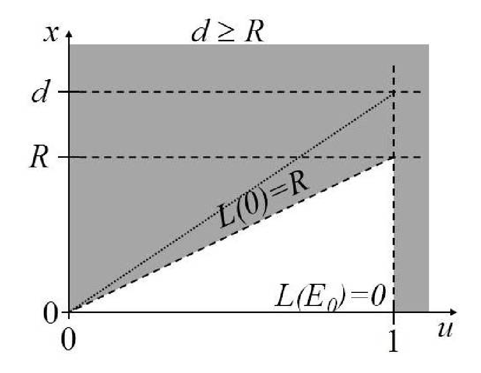
If $d>R$ the variable $x$ can explore the interval $x\in\left[0,R\right]$ . This is the case of the PHS in Figure 17, where $d=4\,\mu m$ , $R_{Li(830KeV)}=1.7\,\mu m$ and $R_{\alpha(1470KeV)}=3.4\,\mu m$ . We take the two particles of the $94\%$ branching ratio of ${}^{10}B$ reaction as example.
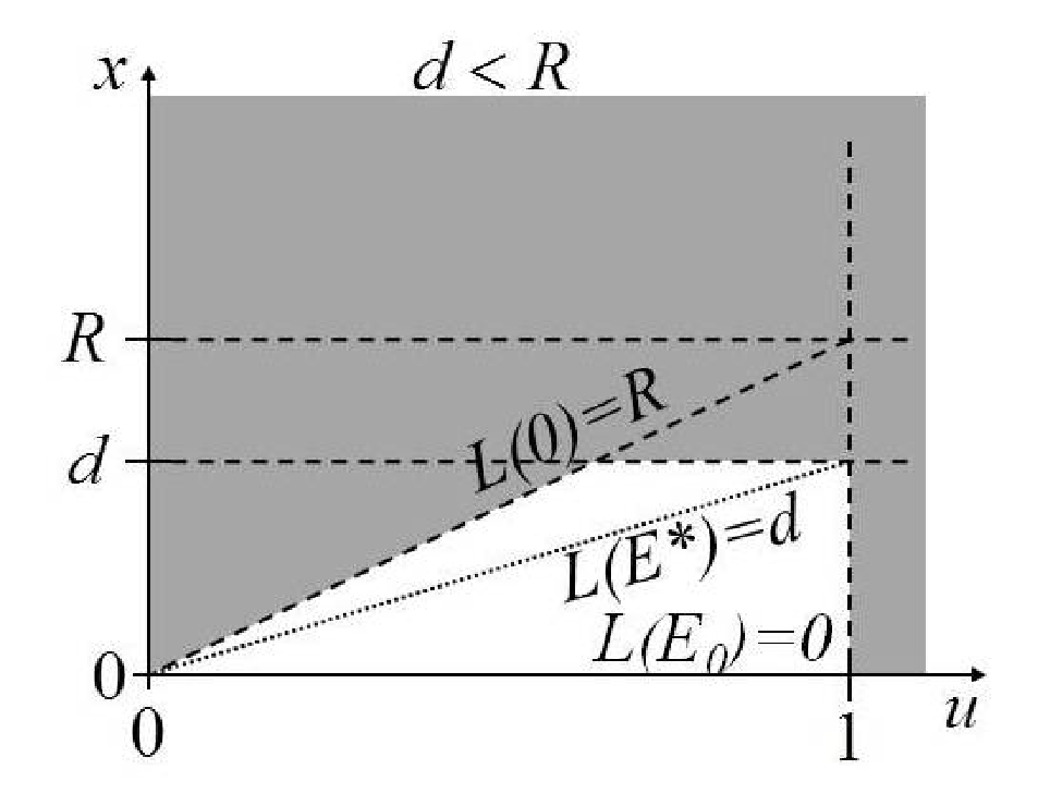
If $d<R$ , the variable $x$ can explore the interval $x\in\left[0,d\right]$ (see Figure 19), thus the domain is now a trapezoid. The events near the line $\frac{x}{u}=L(E^{*})=d$ , which is the switching condition found in the Equations 46 and 47, give rise to a peak because this line has the maximum length available. Thus, we expect a peak in the PHS around $E^{*}$ . This is shown in Figure 16 where $d=1\,\mu m$ and, again, $R_{Li(830KeV)}=1.7\,\mu m$ and $R_{\alpha(1470KeV)}=3.4\,\mu m$ , the peaks that originate from the condition $\frac{x}{u}=L(E^{*})=d$ for the two particles are indicated by the arrows.
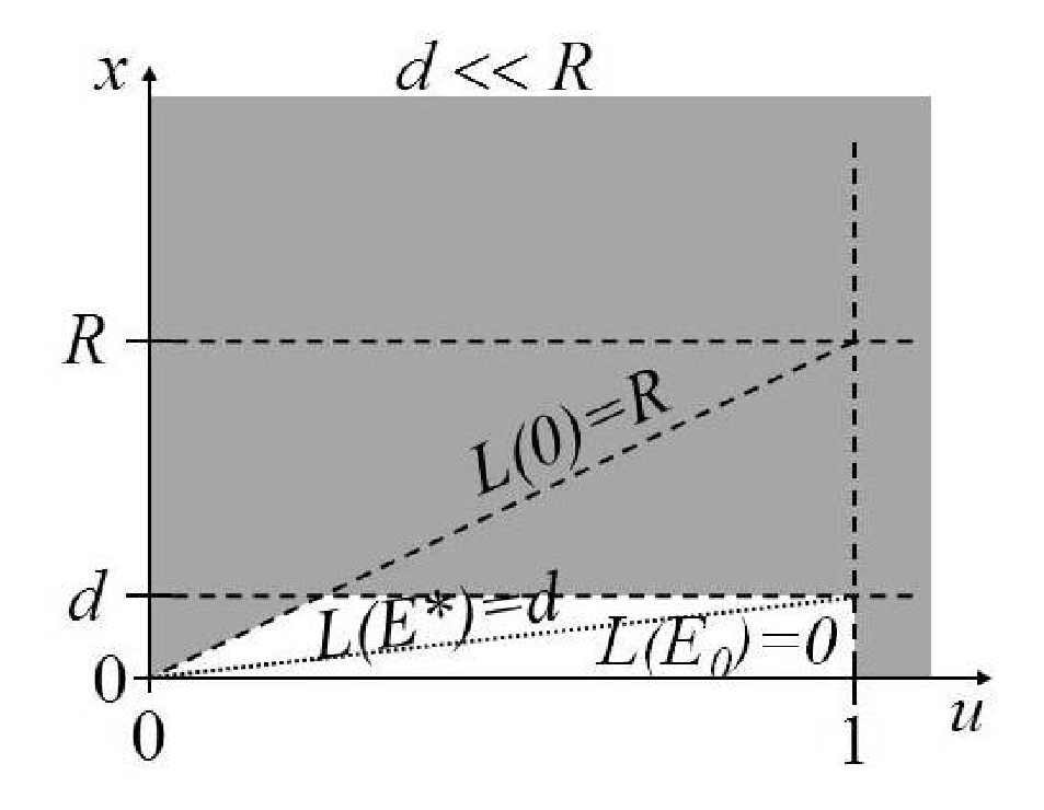
If $d\geq R$ , the peak occurs for $L(E^{*})=R$ , that is, zero energy. This is problematic for $\gamma$ -ray to neutron discrimination.
If $d<<R$ , the variable space is compressed and the straight lines identified by $\frac{x}{u}=L(E^{*})=d$ and $\frac{x}{u}=L(E)=0$ become more and more similar. The two peaks approach and, the more $d$ is negligible compared to $R$ , the more the two peaks appear as one single peak (see Figure 15).
If we want to avoid a strong presence of neutrons in the low energy range of the PHS, where we know the $\gamma$ -rays contamination is strong, it is important to try to get the second peak higher than the energy threshold ( $E_{Th}$ ). This implies that the thickness $d$ of any layer in the detector should obey $d<L(E_{Th})$ for the $L$ corresponding to the particle with the smallest range. This can be a contradictory requirement with efficiency optimization in which case a compromise between $\gamma$ -rays rejection and efficiency has to be found.

4.2 Transmission mode

Equations for transmission mode can be calculated in the same way they have been determined for back-scattering mode by substituting $x$ with $d-y$ in the Expression 38 and $x$ with $y$ in the expression $\delta\left(\frac{x}{u}-L\right)$ . As a result we obtain:

P(L)\,dL=\begin{cases}\frac{1}{2L^{2}}\left(\frac{1}{\Sigma}e^{-\Sigma\cdot d}+(L-\frac{1}{\Sigma})e^{-\Sigma\cdot(d-L)}\right)\,dL&\mbox{if \,}L\leq d\\ \frac{1}{2L^{2}}\left(\frac{1}{\Sigma}e^{-\Sigma\cdot d}+(d-\frac{1}{\Sigma})\right)\,dL&\mbox{if \, }L>d\end{cases}

(48)

Hence, $Q(E)dE$ can be calculated as shown already in Section 4.1.
However the same conclusions can be drawn concerning the qualitative aspects of the PHS, especially the position of the two peaks.

5 Conclusions

We demonstrated that the sputtering technique, suited to make blades with equal coating thickness on both sides of the substrate, is well-adapted to make efficiency optimized blades when the substrate effect can be neglected for any given neutron wavelength and for any incidence angle distribution. Moreover, this result is also valid for a multi-layer detector where several blades are arranged in cascade.
Analytical formulae have been derived in order to optimize the coating thicknesses of blades in single-blade and in multi-layer detectors.
The blade-by-blade optimization in the case of a multi-layer detector for a single neutron wavelength can achieve a few percent more efficiency over the same blade optimization but this can lead to several blades less in the detector. Moreover, in the case of a distribution of wavelengths, the suited optimization from a distribution does not give important improvements in the overall efficiency compared with a monochromatic optimization done for the barycenter of the distribution. On the other hand, the optimization of the efficiency for a neutron wavelength distribution is often more balanced between short and long wavelengths than the barycenter optimization.
We have demonstrated that for our model the analytical expression for the PHS is in a good agreement with measurements. Moreover, thanks to this model, we understood the overall shape of the PHS which can be important if one wants to improve the $\gamma$ -ray to neutron discrimination in neutron detectors.

6 Outlook

Even though the substrate effect can be neglected in most cases when dealing with a small amount of blades, its effect in a multi-layer detector can strongly differ from the results obtained for the ideal case of completely transparent substrate. A further step is to take its effect into account.

Appendix A Formulae in [11]

The relations between the formulae in [11] and the expression used in this paper are the following:

•

the particles ranges $L$ are denoted by $R$ ;
•

the branching ratios of the ${}^{10}B$ reaction (expressed by $F_{p}$ ) are $F_{1}=0.94$ and $F_{2}=0.06$ ;
•

the thickness of the layer is $d=D_{F}$ .

Hence, the relation between the expressions 1, 2, 5 and the formulae in [11] is:

	$\displaystyle\varepsilon_{T}(d_{T})$	$\displaystyle=0.94\cdot\varepsilon_{T}(R^{94\%}_{1},R^{94\%}_{2})+0.06\cdot\varepsilon_{T}(R^{6\%}_{1},R^{6\%}_{2})=$		(49)
		$\displaystyle=S_{1}(D_{F},L_{1},0.94)+S_{1}(D_{F},L_{2},0.94)+S_{2}(D_{F},L_{1},0.06)+S_{2}(D_{F},L_{2},0.06)$		(49)

Valid for both equations ( $18a$ ) ( $D_{F}\leq L_{i}$ ) and ( $18b$ ) ( $D_{F}>L_{i}$ ) in Section $4.2$ of [11]. In the case of the back-scattering mode, equations ( $25a$ ) and ( $25b$ ) in [11], we consider one layer of converter and we replace $\varepsilon_{T}(d_{T})$ into $\varepsilon_{BS}(d_{BS})$ in the expression for back-scattering.
In a different way, for both equations ( $18a$ ) and ( $18b$ ), we can also write:

F_{p}\cdot\varepsilon_{T}=S_{p}(D_{F},L_{1},F_{p})+S_{p}(D_{F},L_{2},F_{p})

(50)

Appendix B Formulae in [12]

The relations between the formulae in [12] and the expression used in this paper are the following:

•

the macroscopic cross-section ( $\Sigma$ ) is expressed in terms of mean free path $l=\frac{1}{\Sigma}$ ;
•

the variable $u$ is denoted by its cosine $u=\cos(\theta)$ ;

The formulae $(4)$ in [12] corresponds to the Equation 38, unless a factor $\frac{1}{2}$ , where $l=\frac{1}{\Sigma}$ .
The formulae $(3)$ in [12] corresponds to the Equation 39.

Acknowledgements.

The authors would like to thank J. Correa and A. Khaplanov for the data and the Thin Film Physics Division - Linköping University, (Sweden) - especially C. Höglund, - for the coatings and B. Guérard, thesis advisor of one of the authors (F. P.), to have given the opportunity to have worked on this subject.

References

[1] J. Birch et al., ${}^{10}B_{4}C$ Multi-Grid as an Alternative to ${}^{3}He$ for large area neutron detectors, IEEE T. Nucl. Sci., Volume PP, Issue 99, 17 January 2013, Pages 1-8, ISSN 0018-9499, \hrefhttp://dx.doi.org/10.1109/TNS.2012.2227798 10.1109/TNS.2012.2227798.
[2] M. Henske et al., The 10B based Jalousie neutron detector $-$ An alternative for 3He filled position sensitive counter tubes, Nucl. Instrum. Meth. A, Volume 686, 11 September 2012, Pages 151-155, ISSN 0168-9002, \hrefhttp://dx.doi.org/10.1016/j.nima.2012.05.075 10.1016/j.nima.2012.05.075.
[3] J.C. Buffet et al., Study of a 10B-based Multi-Blade detector for Neutron Scattering Science, IEEE T. Nucl. Sci. Conference Record - Anaheim, 2012.
[4] J. L. Lacy et al., Boron-coated straws as a replacement for 3He-based neutron detectors, Nucl. Instrum. Meth. A, Symposium on Radiation Measurements and Applications (SORMA) XII 2010, Volume 652, Issue 1, 2011, Pages 359-363, ISSN 0168-9002, \hrefhttp://dx.doi.org/10.1016/j.nima.2010.09.01110.1016/j.nima.2010.09.011.
[5] R. T. Kouzes et al., Neutron detection alternatives to 3He for national security applications, Nucl. Instrum. Meth. A, Volume 623, Issue 3, 2010, Pages 1035-1045, ISSN 0168-9002, \hrefhttp://dx.doi.org/10.1016/j.nima.2010.08.021 10.1016/j.nima.2010.08.021.
[6] B. Gebauer et al., Towards detectors for next generation spallation neutron sources, Proceedings of the 10th International Vienna Conference on Instrumentation, Nucl. Instrum. Meth. A, Volume 535, Issues 1-2, 2004, Pages 65-78, ISSN 0168-9002, \hrefhttp://dx.doi.org/10.1016/j.nima.2004.07.266 10.1016/j.nima.2004.07.266.
[7] A. Athanasiades et al., Straw detector for high rate, high resolution neutron imaging, Nuclear Science Symposium Conference Record, 2005 IEEE, Volume 2, Pages 623-627, 10.1109/NSSMIC.2005.1596338.
[8] D.S. McGregor et al., Semi-insulating bulk GaAs as a semiconductor thermal-neutron imaging device, Nucl. Instrum. Meth. A, Volume 380, Issues 1-2, 1996, Pages 271-275, ISSN 0168-9002, \hrefhttp://dx.doi.org/10.1016/S0168-9002(96)00347-6 10.1016/S0168-9002(96)00347-6.
[9] K. Tsorbatzoglou et al., Novel and efficient 10B lined tubelet detector as a replacement for 3He neutron proportional counters, Symposium on Radiation Measurements and Applications (SORMA) XII 2010, Nucl. Instrum. Meth. A, Volume 652, Issue 1, 2010, Pages 381-383, ISSN 0168-9002, \hrefhttp://dx.doi.org/10.1016/j.nima.2010.08.102 10.1016/j.nima.2010.08.102.
[10] J. L. Lacy et al., One meter square high rate neutron imaging panel based on boron straws, Nuclear Science Symposium Conference Record (NSS/MIC), 2009 IEEE, Pages 1117-1121, ISSN 1095-7863, \hrefhttp://ieeexplore.ieee.org/stamp/stamp.jsp?tp=arnumber=5402421isnumber=5401554 10.1109/NSSMIC.2009.5402421.
[11] D.S. McGregor et al., Design considerations for thin film coated semiconductor thermal neutron detectors $-I$ : basics regarding alpha particle emitting neutron reactive films, Nucl. Instrum. Meth. A, Volume 500, Issues 1-3, 11 March 2003, Pages 272-308, ISSN 0168-9002, \hrefhttp://dx.doi.org/10.1016/S0168-9002(02)02078-8 10.1016/S0168-9002(02)02078-8.
[12] D.J. Salvat et al., A boron-coated ionization chamber for ultra-cold neutron detection, Nucl. Instrum. Meth. A, Volume 691, 1 November 2012, Pages 109-112, ISSN 0168-9002, \hrefhttp://dx.doi.org/10.1016/j.nima.2012.06.041 10.1016/j.nima.2012.06.041.
[13] C. Höglund et al., $B_{4}C$ thin films for neutron detection, J. Appl. Phys., Volume 111, Issue 10, 23 May 2012, Pages 10490-8, ISSN 0168-9002, \hrefhttp://link.aip.org/link/?JAP/111/104908/110.1063/1.4718573.
[14] V. F. Sears, Neutron scattering lengths and cross sections - Special Feature, Neutron News, Volume 3, Issue 3, 1992, Pages 29-37.
[15] T. Bigault et al., 10B multi-grid proportional gas counters for large area thermal neutron detectors, Neutron News, Volume 23, Issue 4, 2012, Pages 20-25, \hrefhttp://www.tandfonline.com/doi/abs/10.1080/10448632.2012.72532910.1080/10448632.2012.725329.
[16] Z. Wang et al., Multi-layer boron thin-film detectors for neutrons, NNucl. Instrum. Meth. A, Volume 652, Issue 1, 1 October 2011, Pages 323-325, ISSN 0168-9002, \hrefhttp://dx.doi.org/10.1016/j.nima.2011.01.13810.1016/j.nima.2011.01.138.
[17] M.Klein et al., CASCADE, neutron detectors for highest count rates in combination with ASIC/FPGA based readout electronics, Nucl. Instrum. Meth. A, VCI 2010 Proceedings of the 12th International Vienna Conference on Instrumentation, Volume 628, Issues 1, 2011, Pages 9-18, ISSN 0168-9002, \hrefhttp://dx.doi.org/10.1016/j.nima.2010.06.27810.1016/j.nima.2010.06.278.
[18] J.F. Ziegler et al., SRIM - The stopping and range of ions in matter (2010), Nucl. Instrum. Meth. B, Volume 268, 2010, Pages 1818-1823, \hrefhttp://dx.doi.org/10.1016/j.nimb.2010.02.091 10.1016/j.nimb.2010.02.091.