Efficient parallel coordinate descent algorithm for convex optimization problems with separable constraints: application to distributed MPC Note: The research leading to these results has received funding from: the European Union, Seventh Framework Programme (FP7/2007–2013) under grant agreement no 248940; CNCSIS-UEFISCSU (project TE, no. 19/11.08.2010); ANCS (project PN II, no. 80EU/2010); Sectoral Operational Programme Human Resources Development 2007-2013 of the Romanian Ministry of Labor, Family and Social Protection through the Financial Agreement POSDRU/89/1.5/S/62557.
Abstract
In this paper we propose a parallel coordinate descent algorithm for solving smooth convex optimization problems with separable constraints that may arise e.g. in distributed model predictive control (MPC) for linear network systems. Our algorithm is based on block coordinate descent updates in parallel and has a very simple iteration. We prove (sub)linear rate of convergence for the new algorithm under standard assumptions for smooth convex optimization. Further, our algorithm uses local information and thus is suitable for distributed implementations. Moreover, it has low iteration complexity, which makes it appropriate for embedded control. An MPC scheme based on this new parallel algorithm is derived, for which every subsystem in the network can compute feasible and stabilizing control inputs using distributed and cheap computations. For ensuring stability of the MPC scheme, we use a terminal cost formulation derived from a distributed synthesis. Preliminary numerical tests show better performance for our optimization algorithm than other existing methods.
Keywords:
Coordinate descent optimization, parallel algorithm, (sub)linear convergence rate, distributed model predictive control, embedded control.1 Introduction
Model predictive control (MPC) has become a popular advanced control technology implemented in network systems due to its ability to handle hard input and state constraints [20]. Network systems are usually modeled by a graph whose nodes represent subsystems and whose arcs indicate dynamic couplings. These types of systems are complex and large in dimension, whose structures may be hierarchical and they have multiple decision-makers (e.g. process control [21], traffic and power systems [7, 25], flight formation [13]).
Decomposition methods represent a very powerful tool for solving distributed MPC problems in network systems. The basic idea of these methods is to decompose the original large optimization problem into smaller subproblems. Decomposition methods can be divided in two main classes: primal and dual decomposition methods. In primal decomposition the optimization problem is solved using the original formulation and variables via methods such as interior-point, feasible directions, Gauss-Jacobi type and others [3, 5, 6, 23, 25]. In dual decomposition the original problem is rewritten using Lagrangian relaxation for the coupling constraints and the dual problem is solved with a Newton or (sub)gradient algorithm [1, 2, 4, 16, 15]. In [23, 25] cooperative based distributed MPC algorithms are proposed based on Gauss-Jacobi iterations, where asymptotic convergence to the centralized solution and feasibility for their iterates is proved. In [5, 6] non-cooperative algorithms are derived for distributed MPC problems, where communication takes place only between neighbors. In [3] a distributed algorithm based on interior-point methods is proposed whose iterates converge to the centralized solution. In [1, 4, 16, 15] dual distributed gradient algorithms based on Lagrange relaxation of the coupling constraints are presented for solving MPC problems, algorithms which usually produce feasible and optimal primal solutions in the limit. While much research has focused on a dual approach, our work develops a primal method that ensures constraint feasibility, has low iteration complexity and provides estimates on suboptimality.
Further, MPC schemes tend to be quite costly computation-wise compared with classical control methods, e.g. PID controllers, so that for these advanced schemes we need hardware with a reasonable amount of computational power that is embedded on the subsystems. Therefore, research for distributed and embedded MPC has gained momentum in the past few years. The concept behind embedded MPC is designing a control scheme that can be implemented on autonomous electronic hardware, e.g programmable logic controllers (PLC) [24] or field-programmable gate arrays (FPGAs) [10]. Such devices vary widely in both computational power and memory storage capabilities as well as cost. As a result, there has been a growing focus on making MPC schemes faster by reducing problem size and improving the computational efficiency through decentralization [21], moving block strategies (e.g. by using latent variables [8] or Laguerre functions [27]) and other procedures, allowing these schemes to be implemented on cheaper hardware with little computational power.
The main contribution of this paper is the development of a parallel coordinate descent algorithm for smooth convex optimization problems with separable constraints that is computationally efficient and thus suitable for MPC schemes that need to be implemented distributively or in hardware with limited computational power. This algorithm employs parallel block-coordinate updates for the optimization variables and has similarities to the optimization algorithm proposed in [23], but with simpler implementation, lower iteration complexity and guaranteed rate of convergence. We derive (sub)linear rate of convergence for the new algorithm whose proof relies on the Lipschitz property of the gradient of the objective function. The new parallel algorithm is used for solving MPC problems for general linear network systems in a distributed fashion using local information. For ensuring stability of the MPC scheme, we use a terminal cost formulation derived from a distributed synthesis and we eliminate the need for a terminal state constraint. Compared with the existing approaches based on an end point constraint, we reduce the conservatism by combining the underlying structure of the system with distributed optimization [9, 12, 19]. Because the MPC optimization problem is usually terminated before convergence, our MPC controller is a form of suboptimal control. However, using the theory of suboptimal control [22] we can still guarantee feasibility and stability.
This paper is organized as follows. In Section 2 we derive our parallel coordinate descent optimization algorithm and prove the convergence rate for it. In Sections 3.1-3.2 we introduce the model for general network systems, present the MPC problem with a terminal cost formulation and provide the means for which this terminal cost can be synthesized distributively. In Sections 3.3-3.4 we employ our algorithm for distributively solving MPC problems arising from network systems and discuss details regarding its implementation. In Section 4 we compare its performance with other algorithms and test it on a real application - a quadruple water tank process.
2 A parallel coordinate descent algorithm for smooth convex problems with separable constraints
We work in composed by column vectors. For we denote the standard Euclidean inner product , the Euclidean norm and . Further, for a symmetric matrix , we use for a positive (semi)definite matrix. For matrices and , we use to denote the block diagonal matrix formed by these two matrices.
In this section we propose a parallel coordinate descent based algorithm for efficiently solving the general convex optimization problem of the following form:
| (1) |
where with , are the decision variables, constrained to individual convex sets . We gather the individual constraint sets into the set , and denote the entire decision variable for (1) by , with . As we will show in this section, the new algorithm can be used on many parallel computing architectures, has low computational cost per iteration and guaranteed convergence rate. We will then apply this algorithm for solving distributed MPC problems arising in network systems in Section 3.
2.1 Parallel Block-Coordinate Descent Method
Let us partition the identity matrix in accordance with the structure of the decision variable :
where for all . With matrices we can represent . We also define the partial gradient of as: . We assume that the gradient of is coordinate-wise Lipschitz continuous with constants , i.e:
| (2) |
Due to the assumption that is coordinate-wise Lipschitz continuous, it can be easily deduced that [17]:
| (3) |
We now introduce the following norm for the extended space :
| (4) |
which will prove useful for estimating the rate of convergence for our algorithm. Additionally, if function is smooth and strongly convex with regards to with a parameter , then [18]:
| (5) |
Note that if is strongly convex w.r.t the standard Euclidean norm with a parameter , then , where . By taking and in (5) we also get:
and combining with (3) we also deduce that .
We now define the constrained coordinate update for our algorithm:
The optimality conditions for the previous optimization problem are:
| (6) |
Taking in the previous inequality and combining with (3) we obtain the following decrease in the objective function:
| (7) |
We now present our Parallel Coordinate Descent Method, that resembles the method in [23] but with simpler implementation, lower iteration complexity and guaranteed rate of convergence, and is a parallel version of the coordinate descent method from [17]:
Algorithm PCDM Choose for all . For : 1. Compute in parallel 2. Update in parallel:
Note that if the sets are simple (by simple we understand that the projection on these sets is easy), then computing consists of projecting a vector on these sets and can be done numerically very efficient. For example, if these sets are simple box sets, i.e , then the complexity of computing , once is available, is . In turn, computing has, in the worst case, complexity for quadratic dense functions. Thus, Algorithm PCDM has usually a very low iteration cost per subsystem compared to other existing methods, e.g. Jacobi type algorithm presented in [23], which usually require numerical complexity at least per iteration for each subsystem , provided that the local quadratic problems are solved with an interior point solver. Also, in the following two theorems we provide estimates for the convergence rate of our algorithm, while for the algorithm in [23] only asymptotic convergence is proved.
From (6)-(7), convexity of and we see immediately that method PCDM decreases strictly the objective function at each iteration, provided that , where is the optimal solution of (1), i.e.:
| (8) |
Let be the optimal value in optimization problem (1). The following theorem derives convergence rate of Algorithm PCDM and employs standard techniques for proving rate of convergence of the gradient method [17, 18]:
Theorem 1
where .
Proof 1
We introduce the following term:
where is the optimal solution of (1) and . Then, using similar derivations as in [17], we have:
By convexity of and (3) we obtain:
| (9) |
and adding up these inequalities we get:
Taking into account that our algorithm is a descent algorithm, i.e. for all and by the previous inequality the proof is complete. ∎
Now, we derive linear convergence rate for Algorithm PCDM, provided that is additionally strongly convex:
Theorem 2
Proof 2
We take and in (5) and through (9) we get:
| (10) |
From the strong convexity of in (5) we also get:
We now define and using the previous inequality we obtain the following result:
Using this inequality in (10) we get:
Applying this inequality iteratively, we obtain the following for :
and by replacing we complete the proof. ∎
The following properties follow immediately for our Algorithm PCDM.
Lemma 1
For the optimization problem (1), with
the assumptions of Theorem 2, we have the following statements:
(i) Given any feasible initial guess , the iterates of the
Algorithm PCDM are feasible at each iteration, i.e. for all .
(ii) The function is nonincreasing, i.e. according to (8).
(iii) The sub(linear) rate of convergence of Algorithm PCDM is
given in Theorem 1 (Theorem 2).
3 Application of Algorithm PCDM to distributed suboptimal MPC
The Algorithm PCDM can be used to solve distributively input constrained MPC problems for network systems after state elimination. In this section we show that the MPC scheme obtained by solving approximately the corresponding optimization problem with Algorithm PCDM is stable and distributed.
3.1 MPC for network systems with terminal cost and without end constraints
In this paper we consider discrete-time network systems, which are usually modeled by a graph whose nodes represent subsystems and whose arcs indicate dynamic couplings, defined by the following linear state equations [3, 4, 21]:
| (11) |
where denotes the number of interconnected subsystems, and represent the state and respectively the input of th subsystem at time , , and is the set of indices which contains the index and that of its neighboring subsystems. A particular case of (11), that is frequently found in literature [16, 23, 25], has the following dynamics:
| (12) |
For stability analysis, we also express the dynamics of the entire system: , where , , , and , . For system (11) or (12) we consider local input constraints:
| (13) |
with compact, convex sets with the origin in their interior. We also consider convex local stage and terminal costs for each subsystem : and . Let us denote the input trajectory for subsystem and the overall input trajectory for the entire system by:
We can now formulate the MPC problem for system (11) over a prediction horizon of length and a given initial state as [20]:
| (14) | ||||
It is well-known that by eliminating the states using dynamics (11), the MPC problem (14) can be recast [20] as a convex optimization problem of type (1), where , the function is convex (recall that we assume the stage and final costs and to be convex), whilst the convex sets are the Cartesian product of the convex sets for times. Moreover, in the case of dynamics (12), we can express the objective function of problem (1) as a sum of local functions with sparse structure:
| (15) |
Further, we denote the approximate solution produced by Algorithm PCDM for problem (14) after certain number of iterations with . We also consider that at each MPC step the Algorithm PCDM is initialized (warm start) with the shifted sequence of controllers obtained at the previous step and the feedback controller computed in Section 3.2 below. The suboptimal MPC scheme corresponding to (14) would now be:
Suboptimal MPC scheme Given initial state and initial repeat: 1. Recast MPC problem (14) as opt. problem (1) 2. Solve (1) approximately with Alg. PCDM starting from and obtain 3. Update . Update using warm start.
3.2 Distributed synthesis for a terminal cost
We assume that stability of the MPC scheme (14) is enforced by adapting the terminal cost and the horizon length appropriately such that sufficient stability criteria are fulfilled [9, 12, 19]. Usually, stability of MPC with quadratic stage cost , where the matrices and , and without terminal constraint is enforced if the following criteria hold: there exists a neighborhood of the origin , a stabilizing feedback law and a terminal cost such that we have
| (16) |
where the matrices and have a block diagonal structure and are composed of the blocks and , respectively. As shown in [9, 12, 19], MPC schemes based on the condition (16) are usually less conservative than schemes based on end point constraint. Keeping in line with the distributed nature of our system, the control law and the final stage cost need to be computed locally. In this section we develop a distributed synthesis procedure to construct them locally. We choose the terminal cost for each subsystem to be quadratic: , where . For a locally computed , we employ distributed control laws: , i.e. is taken linear with a block-diagonal structure. Centralized LMI formulations of (16) for quadratic terminal costs are well-known in the literature [20]. However, our goal is to solve (16) distributively. To this purpose, we first need to introduce vectors and for subsystem , where and . These vectors are comprised of the state and input vectors of subsystem and those of its neighbors: .
Since our synthesis procedure needs to be distributed and taking into account that , we impose the following distributed structure to ensure (16) (see also [11] for a similar approach where infinity-norm control Lyapunov functions are synthesized in a decentralized fashion by solving linear programs for each subsystem) for :
| (17) |
such that . We assume that also have a quadratic form, with , where . Being a sum of quadratic functions, can itself be expressed as a quadratic function, , where is formed from the appropriate block components of matrices . Note that we do not require that matrices be negative semidefinite. On the contrary, positive or indefinite matrices allow local terminal costs to increase so long as the global cost still decreases. This approach reduces the conservatism in deriving the matrices and . For obtaining and , we introduce matrices , , , such that and . We now define the matrices , and , as to express the dynamics (11) for subsystem : . Using these notations we can now recast inequality (17) as:
| (18) | ||||
The task of finding suitable , and matrices is now reduced to the following optimization problem:
| (19) |
It can be easily observed that if the optimal value , consequently and (16) holds. This optimization problem, in its current nonconvex form, cannot be solved efficiently. However, it can be recast as a sparse SDP if we can reformulate (18) as an LMI. We need now to make the assumption that all the subsystems have the same dimension for the states, i.e. for all . Subsequently, we introduce the well-known linearizations: and a series of matrices that will be of aid in formulating the LMIs:
where the blocks are of appropriate dimensions11 1 By we denote the identity matrix of size , by we denote the standard Kronecker product and by the cardinality of the set ..
Lemma 2
If the following SDP:
| (20) |
| (21) | ||||
has an optimal value , then (16) holds22 2 By we denote the transpose of the symmetric block of the matrix..
Proof 3
3.3 Stability of the MPC scheme
We can consider the cost function of the MPC problem as a Lyapunov function, using the standard theory for suboptimal control (see e.g. [12, 19, 20, 22, 23] for similar approaches). We also consider that at each MPC step the Algorithm PCDM is initialized (warm start) with the shifted sequence of controllers obtained at the previous step and the feedback controller computed in Section 3.2 such that (16) is satisfied and we denote it by . Assume also that , and are chosen such that, together with the following set
satisfies (16). Then, using Theorem 3 from [12] we have that our MPC controller stabilizes asymptotically the system for all initial states , where
such that , where is a parameter for which we have for all . Clearly, this MPC scheme is locally stable with a region of attraction .
3.4 Distributed implementation of the MPC scheme based on Algorithm PCDM
In this section we discuss some technical aspects for the distributed implementation of the MPC scheme derived above when using Algorithm PCDM to solve the control problem (14). Usually, in the linear MPC framework, the local stage and final cost are taken of the following quadratic form:
where the matrices are positive semidefinite, whilst matrices are positive definite. We also assume that the local constraints sets are polyhedral. In this particular case, the objective function in (14), after eliminating the dynamics, is quadratically strongly convex, having the form [20]:
where is positive definite due to the assumption that all are positive definite. Usually, for the dynamics (11) the corresponding matrices and obtained after eliminating the states are dense and despite the fact that Algorithm PCDM can perform parallel computations (i.e. each subsystem needs to solve small local problems) we need all to all communication between subsystems. However, for the dynamics (12) the corresponding matrices and are sparse and in this case in our Algorithm PCDM we can perform distributed computations (i.e. the subsystems solve small local problems in parallel and they need to communicate only with their neighborhood subsystems as detailed below). Indeed, if the dynamics of the system are given by (12), then
and thus the matrices and have a sparse structure (see also [3]). Let us define the neighborhood subsystems of a certain subsystem as , where , then the matrix has all the block matrices for all and the matrix has all the block matrices for all , for any given subsystem . As a result, we can express the objective function of problem (1) as a sum of local functions with sparse structure:
| (23) |
Thus, the th block components of can be computed using only local information:
| (24) |
Note that in Algorithm PCDM the only parameters that we need to compute are the Lipschitz constants . However, in the MPC problem, does not depend on the initial state and can be computed locally by each subsystem as: . From the previous discussion it follows immediately that the iterations of Algorithm PCDM can be performed in parallel using distributed computations (see (24)).
Further, our Algorithm PCDM has a simpler implementation of the iterates than the algorithm from [23]: in Algorithm PCDM the main step consists of computing local projections on the sets (in the context of MPC usually these sets are simple and the projections can be computed in closed form); while in the algorithm from [23] this step is replaced with solving local dense QP problems with the feasible set given by (even in the context of MPC this local QP problems cannot be solved in closed form and an additional QP solver needs to be used). Finally, the number of iterations for finding an approximate solution can be easily predicted in our Algorithm (see Theorems 1 and 2), while in the algorithm from [23] the authors prove only asymptotic converge.
4 Numerical Results
Since our Algorithm PCDM has similarities with the algorithm from [23], in this section we compare these two algorithms on controlling a laboratory setup with DMPC (4 tank process) and on MPC problems for random network systems of varying dimension.
4.1 Quadruple tank process

To demonstrate the applicability of our Algorithm PCDM, we apply this newly developed method for solving the optimization problems arising from the MPC problem for a process consisting of four interconnected water tanks, see Fig. 1 for the process diagram, whose objective is to control the level of water in each of the four tanks. For this plant, there are two types of system inputs that can be considered: the pump flows, when the ratios of the three way valves are considered fixed, or the ratios of the three way valves, whilst having fixed flows from the pumps. In this paper, we consider the latter option, with the valve ratios denoted by and , such that tanks 1 and 3 have inflows and , while tanks 2 and 4 have inflows and . The simplified continuous nonlinear model of the plant is well known [1]. We use the following notation: are the levels and are the discharge constants of tank , is the cross section of the tanks, , are the three-way valve ratios, both in , while and are the pump flows.
| Param | S | |||||||||||
| Value | 0.02 | 0.58 | 0.54 | |||||||||
| Unit |
The discharge constants , with and the other parameters of the model are determined experimentally from our laboratory setup (see Table 1). We can obtain a linear continuous state-space model by linearizing the nonlinear model at an operating point given by , , , and the maximum inflows from the pumps, with the deviation variables , , :
where , , is the time constant for tank .
Using zero-order hold method with a sampling time of seconds we obtain the discrete time model of type (12), with the partition and . For the input constraints of the MPC scheme we consider the practical constraints of the ratios of the three way valves for our plant, i.e , where is the linearization input. Due to the fact that our plant has overflow sensors fitted to the tanks and an emergency shutoff program, we do not introduce constraints for the states. For the stage cost we have taken the weighting matrices to be and .
4.2 Implementation of the MPC scheme using MPI
In this section we underline the benefits of Algorithm PCDM when it is implemented in an appropriate fashion for the quadruple tank MPC scheme. We implemented for comparison, Algorithm PCDM and that of [23]. Both algorithms were implemented in C programming language, with parallelization ensured via MPI and linear algebra operations done with CLAPACK. Algorithm [23] requires solving, at each step, QP problems in parallel, problems which cannot be solved in closed form. For solving these QP problems, we use the qpip routine of the QPC toolbox [26]. The algorithms were implemented on a PC, with 2 Intel Xeon E5310 CPUs at 1.60 GHz and 4Gb of RAM. For the MPC problem in this subsection we control the plant such that the levels and inputs will reach those of the steady state linearization values and .
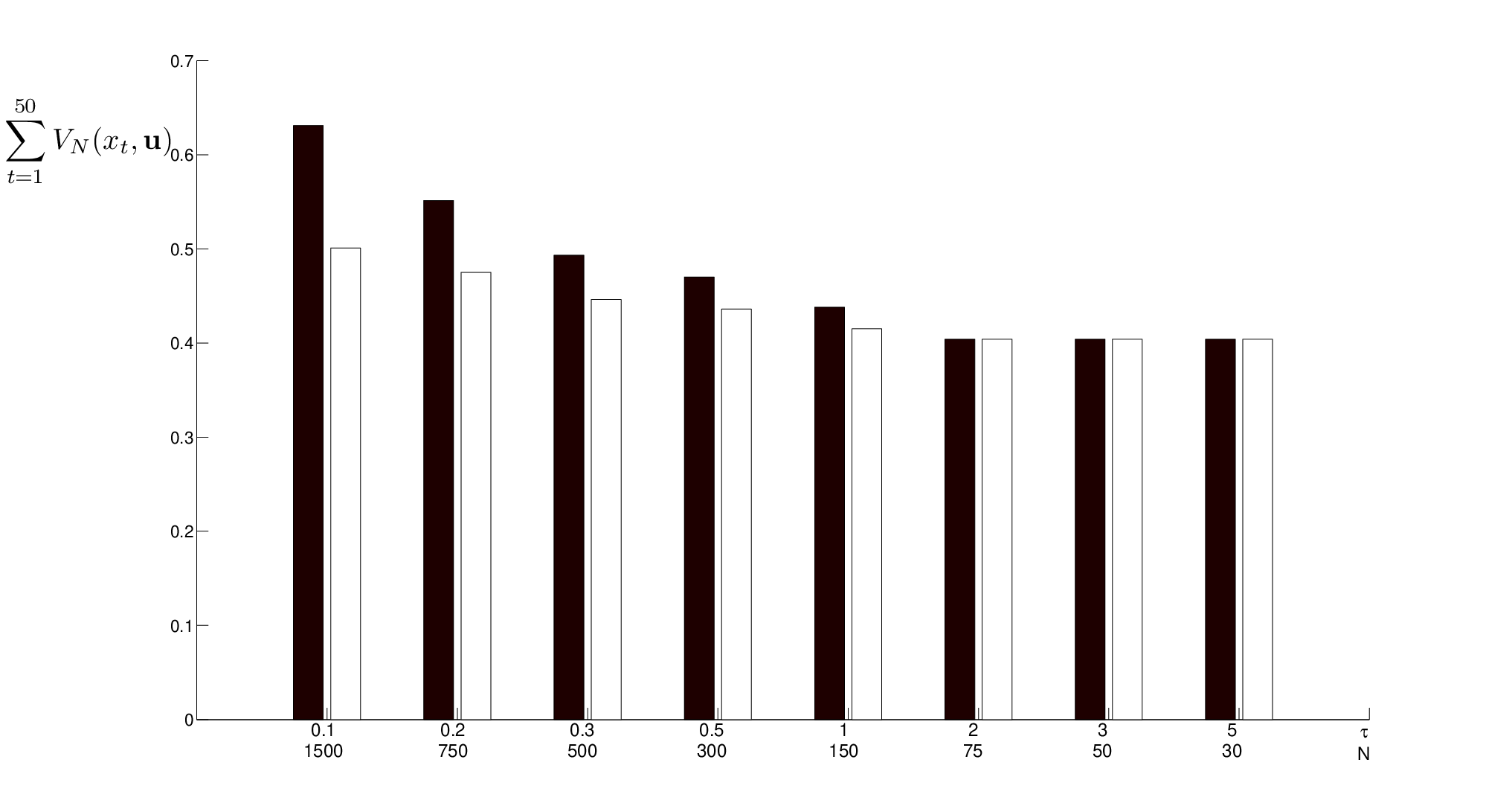
Figure 2 outlines a comparison of the two algorithms for solving this quadruple tank MPC problem, considering a prediction time of seconds, for different prediction horizons and sampling time , such that seconds. The bar values represent the total sum for MPC steps, where is calculated either with PCDM or with the algorithm from [23]. For the same simulation steps, we outline in Table 2 a comparison of the average number of iterations achieved by both algorithms and the performance loss, i.e. a percentile difference between the suboptimal cost achieved in Figure 2 () and the optimal costs that were precalculated with Matlab’s quadprog (), both for the time and prediction horizon . Note that our total cost is usually better than that of [23] when the available time is short () and for both algorithms solve the corresponding optimization problem exactly. Also note that, due to its low complexity iteration, our algorithm performs more than ten times the amount of iterations than the algorithm from [23].
| PCDM | [23] | ||
|---|---|---|---|
| N | Iter / Perf. Loss (%) | Iter / Perf. Loss (%) | |
| 0.1 | 1500 | 7 / 23.9 | 1 / 60.18 |
| 0.2 | 750 | 30 / 17.59 | 2 / 36.48 |
| 0.3 | 500 | 240 / 10.42 | 5 / 22.1 |
| 0.5 | 300 | 1803 / 7.94 | 22 / 16.36 |
| 1 | 150 | 12244 / 2.74 | 258 / 8.44 |
| 2 | 75 | 67470 / 0 | 2495 / 0 |
| 3 | 50 | 153850 / 0 | 8663 / 0 |
| 5 | 30 | 382810 / 0 | 38110 / 0 |
4.3 Implementation of the MPC scheme using Siemens S7-1200 PLC
Due to the limitations, in both hardware and programming language, of the S7-1200 PLC, a proper implementation of any distributed optimization algorithm, in the sense of distributed computations and passing information between processes running on different cores, cannot be undertaken on it. However, to illustrate the fact that our PCDM algorithm is suitable for control devices with limited computational power and memory, we implemented it in a centralized manner for an MPC scheme in order to control the quadruple tank plant. We note that S7-1200 PLC is considered an entry-level PLC, with KB of main memory, MB of load memory (mass storage) and KB of backup memory. There are two main function blocks for the algorithm itself, one that updates in the quadratic objective function given the current levels of the four tanks and one in which Algorithm PCDM is implemented for solving problem (1). Both blocks contain Structured Control Language which corresponds to IEC 1131.3 standard. The remaining function blocks are used for converting the I/O for the plant to corresponding metric values. The elements of the problem which occupy the most memory is the matrix of the objective function and matrix for updating . Both matrices are precomputed offline using Matlab and then stored in the work memory using Data Blocks. The components of the problem which require updating are the input trajectory vectors and the vector of the objective function which is dependent of the current state of the plant and of the current set point. The evolution of the tank levels and input ratios of the plant are recorded in Matlab on the plant’s PC workstation, via an OPC server and Ethernet connection. In accordance with the imposed sample time of seconds, the cycle time of the S7-1200 PLC is also limited to this interval.
| Cycle Time | 5 s | ||
|---|---|---|---|
| Prediction Horizon | 10 | 20 | 30 |
| Maximum Number of Iter. | 104 | 39 | 15 |
| Used Memory (%) | 59 | 72 | 88 |
Due to this cycle time, the limited size of the S7-1200’s work memory and its processing speed, the number of iterations of the Algorithm PCDM that can be computed are also limited. In Table 3 the number of iterations available per prediction horizon, included in the seconds cycle time, and the memory requirements for these prediction horizons are presented. Although the numbers of computed iterations seem small, we have found in practice that the suboptimal MPC scheme still stabilizes the quadruple tank process and ensures set point tracking.


The results of the control process are presented in Fig. 3 for a prediction horizon : the continuous lines represent the evolution of water levels in each of the four tanks, while the dashed lines are their respective set points. We choose two set points. We first let the plant get near its first setpoint, after which we choose a new set point which is an equilibrium point for the plant. As it can be observed from the figure, the MPC scheme still steers the process to the respective set points.
4.4 Implementation of MPC scheme for random network systems
We now wish to outline a comparison of results between algorithm PCDM and that of [23] when solving QP problems arising from MPC for random network systems. Both algorithms were implemented in the same manner as described in Section 4.2. We considered random network systems with dynamics (11) generated as follows: the entries of system matrices and are taken from a normal distribution with zero mean and unit variance. Matrices are then scaled, so that they become neutrally stable. Matrices and are random. The input variables are constrained to lie in box sets whose boundaries are generated randomly. The terminal cost matrices are taken to be the solution of the SDP problem given in Lemma 2. For each subsystem the number of inputs is taken or . We let the prediction horizon range between to . The subsystems are arranged in a ring, i.e. . We first considered subsystems, matching the number of cores on our PC. Parallel implementation was also carried out for subsystems, with each core of the PC running two processes. The resulting random QP problems have variables. The stopping criterion for each algorithm is , with being precomputed for each problem using Matlab’s quadprog. For each prediction horizon, simulations were run, starting from different random initial states.
| PCDM | [23] | PCDM | Quadprog | ||||
|---|---|---|---|---|---|---|---|
| centralized | |||||||
| M | p | CPU (s) | Iter | CPU (s) | Iter | CPU (s) | CPU (s) |
| 8 | 480 | 0.47 | 1396 | 1.904 | 682 | 0.663 | 1.08 |
| 960 | 2.21 | 2839 | 21.52 | 1475 | 9.15 | 3.57 | |
| 3200 | 256.4 | 8671 | 911.2 | 4197 | 265.3 | 39.8 | |
| 4800 | 857.2 | 12750 | 7864.4 | 6182 | 1114 | 139.9 | |
| 9600 | 2223.1 | 16950 | * | * | 3125 | 307.5 | |
| 16 | 480 | 4.36 | 2600 | 4.66 | 1615 | 0.99 | 0.97 |
| 960 | 15.02 | 4792 | 25.18 | 2798 | 14.17 | 3.21 | |
| 3200 | 377.6 | 13966 | 612.8 | 8462 | 423.1 | 41.3 | |
| 4800 | 1524.7 | 23539 | 3061.7 | 14241 | 2161.1 | 134.03 | |
| 9600 | 3415.1 | 29057 | * | * | 4773 | 308.4 | |
Table 4 presents the average CPU time in seconds for the execution of each algorithm. It illustrates that Algorithm PCDM, with its design for distributed computations and simple iterations, usually performs better than that in [23], where the assumption is that for each iteration, a QP problem of size needs to be solved. The entries with denote that the algorithm would have taken over hours to complete. Also note that our implementation of the algorithm from [23], for problems of larger dimensions, i.e starting with , takes less time for it to complete if the problem is divided between subsystems than . This is due to the fact that the solver qpip takes much more time to solve problems of size in the case of and than problems of size for and . Also, the transmission delays between subsystems are negligible in comparison with these qpip times. We have also implemented Algorithm PCDM in a centralized manner, i.e. without using MPI and, as can be seen from the table, we gain speedups of computation when the algorithm is parallelized. Algorithm PCDM is outperformed by Matlab’s quadprog, but do note that quadprog is not designed for distributed implementation and there are no transmission delays between processes.
5 Conclusions
In this paper we have proposed a parallel optimization algorithm for solving smooth convex problems with separable constraints that may arise e.g in MPC for general linear systems comprised of interconnected subsystems. The new optimization algorithm is based on the block coordinate descent framework but with very simple iteration complexity and using local information. We have shown that for strongly convex objective functions it has linear convergence rate. An MPC scheme based on this optimization algorithm was derived, for which every subsystem in the network can compute feasible and stabilizing control inputs using distributed computations. An analysis for obtaining local terminal costs from a distributed viewpoint was made which guarantees stability of the closed-loop interconnected system. Preliminary numerical tests show that this algorithm is suitable for MPC applications, especially those with hardware that has low computational power.
References
- [1] I. Alvarado, D. Limon, D. Munoz de la Pena, J.M. Maestre, M.A. Ridao, H. Scheu, W. Marquardt, R.R. Negenborn, B. De Schutter, F. Valencia, and J. Espinosa, A comparative analysis of distributed MPC techniques applied to the HD-MPC four-tank benchmark, Journal of Process Control, 21(5), 800–815, 2011.
- [2] D.P. Bertsekas and J. Tsitsiklis, Paralel and distributed computation: Numerical Methods, Prentice Hall, 1989.
- [3] E. Camponogara, H.F. Scherer, Distributed Optimization for Model Predictive Control of Linear Dynamic Networks With Control-Input and Output Constraints, IEEE Transactions on Automation Science and Engineering, 8(1), 233–242, 2011.
- [4] M.D. Doan, T. Keviczky and B. De Schutter, A distributed optimization-based approach for hierarchical model predictive control of large-scale systems with coupled dynamics and constraints, Proceedings of Conference on Decision and Control, 5236–5241, 2011.
- [5] W.B. Dunbar, Distributed receding horizon control of dynamicall coupled nonlinear systems, IEEE Transactions on Automatic Control, 52(7), 1249–1263, 2007.
- [6] M. Farina and R. Scattolini, Distributed predictive control: a non-cooperative algorithm with neighbor-to-neighbor communication for linear systems, Automatica, to appear, 2012.
- [7] D. N Godbole, F. H Eskafi and P. P Varaiya, Automated Highway Systems, Proceedings of 13th IFAC World Congress, 121–126, 1996.
- [8] M. Golshan, J.F. MacGregor, M.J. Bruwer and P. Mhaskar, Latent Variable Model Predictive Control (LV-MPC) for trajectory tracking in batch processes, Journal of Process Control, 20(4), 538–550, 2010.
- [9] B. Hu and A. Linnemann, Toward Infinite-Horizon Optimality in Nonlinear Model Predictive Control, IEEE Transactions on Automatic Control, 47(4), 679–682, 2002.
- [10] J.L. Jerez, K.-V. Ling, G.A. Constantinides and E.C. Kerrigan, Model predictive control for deeply pipelined field-programmable gate array implementation: algorithms and circuitry, IET Control Theory and Applications, 6(8), 1029–1041, 2012.
- [11] A. Jokic and M. Lazar, On Decentralized Stabilization of Discrete-time Nonlinear Systems, Proceedings of American Control Conference, 5777–5782, 2009.
- [12] D. Limon, T. Alamo and E.F. Camacho, Stable Constrained MPC without Terminal Constraint, Proceedings of American Control Conference, 4893–4898, 2003.
- [13] P. Massioni and M. Verhaegen, Distributed Control for Identical Dynamically Coupled Systems: A Decomposition Approach, IEEE Transactions on Automatic Control, 54(1), 124–135, 2009.
- [14] M.V. Nayakkankuppam, Solving large-scale semidefinite programs in parallel, Mathematical Programming, 109, 477–504, 2007.
- [15] I. Necoara, V. Nedelcu and I. Dumitrache, Parallel and distributed optimization methods for estimation and control in networks, Journal of Process Control, 21, 756-766, 2011.
- [16] I. Necoara, D. Doan and J. A. K. Suykens, Application of the proximal center decomposition method to distributed model predictive control, Proceedings of the Conference on Decision and Control, 2900–2905, 2008.
- [17] Y. Nesterov, Efficiency of coordinate descent methods on huge-scale optimization problems, SIAM Journal of Optimization, 22(2), 341–362, 2012.
- [18] Y. Nesterov, Introductory Lectures on Convex Optimization: A Basic Course, Kluwer, 2004.
- [19] J.A. Primbs and V. Nevistic, A New Approach to Stability Analysis for Constrained Finite Receding Horizon Control Without End Constraints, IEEE Transactions on Automatic Control, 45(8), 1507–1512, 2000.
- [20] J.B. Rawlings and D.Q. Mayne, Model Predictive Control: Theory and Design, Nob Hill Publishing, 2009.
- [21] R. Scattolini, Architectures for distributed and hierarchical Model Predictive Control – A review, Journal of Process Control, 19(5), 723–731, 2009.
- [22] P.O.M. Scokaert, D.Q. Mayne and J.B. Rawlings, Suboptimal model predictive control (feasibility implies stability), IEEE Transactions on Automatic Control, 44(3), 648–654, 1999.
- [23] B. T. Stewart, A.N. Venkat, J.B. Rawlings, S. Wright and G. Pannocchia, Cooperative distributed model predictive control, Systems & Control Letters, 59, 460–469, 2010.
- [24] G. Valencia-Palomo and J.A. Rossiter Programmable logic controller implementation of an auto-tuned predictive control based on minimal plant information, ISA Transactions, 50, 92–100, 2011.
- [25] A.N Venkat, I.A. Hiskens, J.B Rawlings and S. Wright, Distributed MPC strategies with application to power system automatic generation control, IEEE Transactions on Control Systems Technology, 16(6), 1192–1206, 2008.
- [26] A. Wills, QPC - Quadratic Programming in C, University of Newcastle, Australia, http://sigpromu.org/quadprog/index.html.
- [27] L. Wang, Discrete model predictive control design using Laguerre functions, Journal of Process Control, 14, 131–142, 2004.