Optimized random chemistryThanks: Second author partially supported by National Science Foundation grant DMS-1201312
Abstract.
The random chemistry algorithm of Kauffman can be used to determine an unknown subset of a fixed set . The algorithm proceeds by zeroing in on through a succession of nested subsets . In Kauffman’s original algorithm, the size of each is chosen to be half the size of . In this paper we determine the optimal sequence of sizes so as to minimize the expected run time of the algorithm.
Key words and phrases:
random chemistry algorithm, subset-guessing game1. Introduction
Consider the following set-guessing game between a responder and a questioner. The two players first agree on integers . The game begins with the responder secretly choosing a subset of cardinality . The questioner’s task is to determine . During each turn, the questioner proposes a set ; the responder then indicates whether or not contains . The game ends when the questioner proposes .
In [4], Kauffman proposes a Random Chemistry (RC) algorithm for determining the set when . In following this algorithm, the questioner zeroes in on by choosing successively smaller sets. More precisely, she creates a sequence of sets as follows. Given a set known to strictly contain , the questioner proposes random subsets of of cardinality until she finds one containing . This set is then taken to be .
By allowing the ratios to deviate from a ratio of , we obtain a more general class of algorithms. In Theorem 2 we determine the sequence of ratios that minimizes the expected number of turns in the game.
The above set-guessing problem has appeared in disparate applied contexts. In fact, Kauffman developed his RC algorithm as a way to hypothetically search for auto-catalytic sets of molecules. Eppstein et al. [2] later implemented an RC algorithm as a way of searching for small sets of non-linearly interacting genetic variations in genome-wide association studies. More recently, Eppstein and Hines [3] applied a slight variation of this algorithm to search for collections of multiple outages leading to cascading power failures in models of electrical distribution grids.
A number of closely related problems have also been widely studied. Most notably, the field of group testing (see, for example, [1] for an overview) is also concerned with finding unknown sets. In group testing, a positive test result occurs when the pooled group has a nonempty intersection with the unknown set . In the problem we discuss, a positive test result occurs only when contains all of .
Another class of related problems is that of searching games in which the responder can lie. The Rényi-Ulam game [6, 7] is probably the most famous of these; see [5] for a survey of such games.
In Section 2 we state precisely the optimization problem we are trying to solve. In Section 3 we solve the continuous analog of the problem while Section 4 presents numeric data regarding how well the continuous solution mirrors the discrete one. Section 5 presents an approximate solution to the problem of Section 2 as an application of the calculus of variations.
2. The Optimization Problem
Assume , and are as given as in the Introduction; set and . If we choose a proper subset of of size such that , then
| (1) |
is the probability of obtaining a subset containing . The expected number of times we would have to select a subset of size until we find one containing is therefore .
Now consider a sequence where . Our Generalized Random Chemistry (GRC) algorithm begins by selecting sets of size until we find one, , such that . Such a must exist since, by hypothesis, and . We then select subsets of size from until we find a set containing . The process continues until we have chosen . Define as the probability of selecting a set of size containing from a set of size known to contain . Then, as in (1),
| (2) |
Let the random variable represent the number of selections
needed to find a set containing as described above. Then the
expected value of is ( is a geometric random
variable). Let denote the random variable
representing the total number of selections until we find . This
presents the following
Problem 1.
How should one choose and subject to so as to minimize ?
3. The Continuous Solution
In the combinatorial formulation leading to Problem 1, the are all integers. In this section we relax this requirement and provide an optimal solution when the are only required to be real. Accordingly, we replace the factorial functions with -functions; recall that for a positive integer.
Theorem 2.
The expected number of steps in the GRC algorithm
| (3) |
is minimized over the real numbers for . The optimal value of is , in which case the expression for the reduces to and .
Proof.
Let and note that . Then the problem reduces to finding and that minimize subject to where and for .
The method of Lagrange multipliers instructs us to minimize
| (4) |
where is the Lagrange multiplier. Differentiating with respect to and , setting the derivatives equal to zero and solving gives the solution . To find the optimal value for , note that . This function is minimized when . The optimal values for the probabilities are then and the expected number of steps using the is then . ∎
While Theorem 2 gives closed forms for the optimal values of and the , we do not obtain a simple expression for the . For fixed , the optimal sequence can be obtained by successively solving the equations
| (5) |
The equations are easily solved using a univariate root finding algorithm.
Alternatively, we can modify equation (5) by using the approximation . (This approximation works best for .) In doing so, we find that the optimal values of the are
| (6) |
and that the optimal value of is approximately . As shown in Section 5, this approximate solution can be obtained directly by applying the binomial coefficient approximation to equation (3) and then applying the calculus of variations.
From Theorem 2, the optimal solution has the property that the are constant. The following corollary follows from the well-known fact that a sum of independent, identically distributed geometric random variables has the negative binomial distribution.
Corollary 3.
Fix and . Then the sequence of minimizing induces the distributional property that Negative Binomial where . That is, has probability mass function for .
The utility of Corollary 3 is that it provides a straightforward means for computing the probability that more than steps would be required to find the solution using the optimal sequence.
4. Numerical data
Equation (6) gives a closed form approximate solution to the continuous problem motivated by Problem 1. To utilize this solution in actual problems, we need to map the to integers. A simple method is to provisionally set each according to (6). Then, for set . In this section we will explore several examples in order to show that the integer-valued approximate solutions compare favorably with the continuous minimum of (3).
Example 4.
Let and . The optimal number of partitions given by Theorem 2 is . Using this optimal value for , we computed values for using equations (5) and (6). Figure 1 illustrates the very similar sequences that result. The expected number of steps are for the exact solution and for the approximate solution.
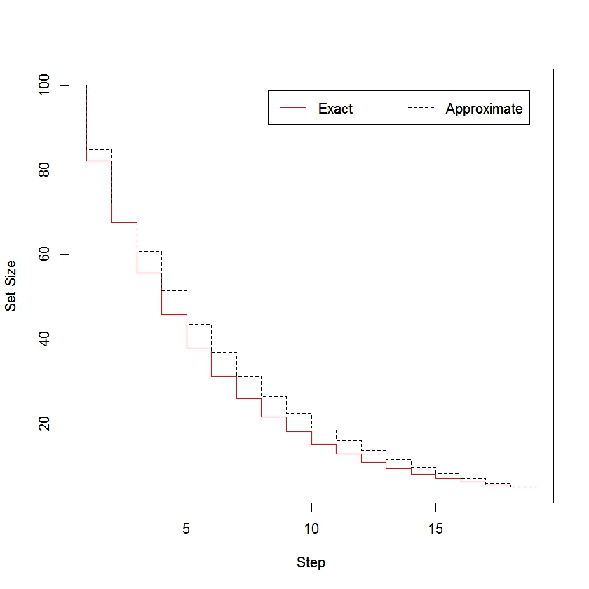
We also simulated runs of the GRC algorithm for the same values of and . In each experiment, we generated a set and counted the number of steps to find it using the optimal sequence on the integer scale. The mean number of steps was . Figure 2 shows the empirical distribution for the number of steps with the negative binomial distribution overlaid.

Finally, in Figure 3 we compare the optimal solution of Theorem 2 to that of Kauffman’s original RC algorithm. Three different -sequences are illustrated for , : The exact solution corresponding to the solution of equation 5 (circles), the approximate solution of 6 (squares), and the sequence generated by Kauffman’s RC algorithm (triangles). The paired increasing plots illustrate the cumulative expected number of guesses required to find a given set .
5. Calculus of Variations
In this section we present an alternate derivation of the approximately optimal formula for the given in (6). In passing from the discrete to the continuous, we can hope that an optimal solution to
yields a good solution to the original sum.
The calculus of variations is designed for exactly this sort of problem: It can be used to find functions that are extrema of the integral
In this case we would set . Unfortunately, it is not clear that the required computation is tractable. So we use the aforementioned approximation
| (7) |
In order to write the righthand side of (7) in the form , we use the approximation . Simple algebra then shows that . Hence we can set . Euler’s equation then tells us that we should look for solutions to the differential equation
Straightforward computations yield
One family of solutions will be those satisfying , i.e., . However, these are increasing functions so we ignore them. Other solutions are those satisfying
This is satisfied by those for which or,
equivalently, those for which is a constant. This implies
.
The constraints and imply that our approximate solution is
By setting , it follows that we can set , as seen in equation (6).
6. Acknowledgments
We wish to thank Jeff Dinitz, Margaret J. Eppstein, Stuart Kauffman and Mark Wagy for helpful discussions leading to this paper.
References
- [1] Ding-Zhu Du and Frank K. Hwang. Combinatorial group testing and its applications, volume 12 of Series on Applied Mathematics. World Scientific Publishing Co. Inc., River Edge, NJ, second edition, 2000.
- [2] M. J. Eppstein, J. L. Payne, B. C. White, and J. H. Moore. Genomic mining for complex disease traits with ’random chemistry’. Genetic Programming and Evolvable Machines, 8:395–411, 2007.
- [3] M.J. Eppstein and P.D.H. Hines. A “random chemistry” algorithm for identifying collections of multiple contingencies that initiate cascading failure. Power Systems, IEEE Transactions on, 27(3):1698–1705, aug. 2012.
- [4] S. Kauffman. At Home in the Universe:The Search for the Laws of Self-Organization and Complexity, pages 145–147. Oxford University Press, USA, 1996.
- [5] Andrzej Pelc. Searching games with errors—fifty years of coping with liars. Theoret. Comput. Sci., 270(1-2):71–109, 2002.
- [6] A. Rényi. On a problem of information theory. MTA Mat. Kut. Int. Kozl., 6B:505–516, 1961.
- [7] S. M. Ulam. Adventures of a Mathematician. Scribner, New York, 1976.