Hypergraph Automata: A Theoretical Model for Patterned Self-assembly
Abstract
Patterned self-assembly is a process whereby coloured tiles self-assemble to build a rectangular coloured pattern. We propose self-assembly (SA) hypergraph automata as an automata-theoretic model for patterned self-assembly. We investigate the computational power of SA-hypergraph automata and show that for every recognizable picture language, there exists an SA-hypergraph automaton that accepts this language. Conversely, we prove that for any restricted SA-hypergraph automaton, there exists a Wang Tile System, a model for recognizable picture languages, that accepts the same language. The advantage of SA-hypergraph automata over Wang automata, acceptors for the class of recognizable picture languages, is that they do not rely on an a priori defined scanning strategy.
1 Introduction
DNA-based self-assembly is an autonomous process whereby a disordered system of DNA sequences forms an organized structure or pattern as a consequence of Watson-Crick complementarity of DNA sequences, without external direction. A DNA-tile-based self-assembly system starts from DNA “tiles”, each of which is formed beforehand from carefully designed single-stranded DNA sequences which bind via Watson-Crick complementarity and ensure the tiles’ shape (square) and structure. In particular, the sides and interior of the square are double-stranded DNA sequence, while the corners have protruding DNA single strands that act as “sticky ends”. Subsequently, the individual tiles are mixed together and interact locally via their sticky-ends to form DNA-based supertiles whose structure is dictated by the base-composition of the individual tiles’ sticky ends. Winfree [15] introduced the abstract Tile Assembly Model (aTAM) as a mathematical model for tile-based self-assembly systems. Ma [13] introduced the patterned self-assembly of single patterns, whereby coloured tiles self-assemble to build a particular rectangular coloured pattern. Patterned self-assembly models a particular type of application in which tiles may differ from each other by some distinguishable properties, modelled as colours [14, 2]. Orponen [7, 10] designed several algorithms to find the minimum tile set required to construct one given coloured pattern. Czeizler [4] proved that this minimization problem is NP-hard.
In this paper, we propose self-assembly (SA) hypergraph automata as a general model for patterned self-assembly and investigate its connections to other models for two-dimensional information and computation, such as 2D (picture) languages and Wang Tile Systems. A 2D (picture) language consists of 2D words (pictures), defined as mappings from the points in the two-dimensional space to a finite alphabet of cardinality . Here, denotes the set . Note that, if we take the alphabet to be a set of colours, the definition of a picture is analogous to that of a coloured pattern [13].
Early generating/accepting systems for 2D languages comprise tiles [6], 2D automata [3], two-dimensional on-line tessellation acceptors [8], and 2D grammars. More recently a generating system was introduced by Varricchio [5] that used Wang tiles. A Wang tile system [5] is a specialized tile-based model that generates the class of recognizable picture languages, a subclass of the family of 2D languages. The class of recognizable picture languages is also accepted by Wang automata, a model introduced in [11]. Like other automata for 2D languages [1], Wang tile automata use an explicit pre-defined scanning strategy [12] when reading the input picture and the accepted language depends on the scanning strategy that is used. Due to this, Wang automata are a suboptimal model for self-assembly. Indeed, if we consider the final supertile as given, the order in which tiles are read is irrelevant. On the other hand, if we consider the self-assembly process which results in the final supertile, an “order of assembly” cannot be pre-imposed. In contrast to Wang automata, SA-hypergraph automata are scanning-strategy-independent.
SA-hypergraph automata are a modification of the hypergraph automata introduced by Rozenberg [9] in 1982. An SA-hypergraph automaton (Section ) accepts a language of labelled “rectangular grid graphs”, wherein the labels are meant to capture the notion of colours used in patterned self-assembly. An SA-hypergraph automaton consists of an underlying labelled graph (labelled nodes and edges) and a set of hyperedges, each of which is a subset of the set of nodes of the underlying graph. Intuitively, the hyperedges are meant to model tiles or supertiles while the underlying graph describes how these can attach to each other, similar to a self-assembly process.
We investigate the computational power of SA-hypergraph automata and prove that for every recognizable picture language there is an SA-hypergraph automaton that accepts (Thm. 5.1). Moreover, we prove that for any restricted SA-hypergraph automaton, there exists a Wang tile system that accepts the same language of coloured patterns (Thm. 5.2). Here, restricted SA-hypergraph automaton means an SA-hypergraph automaton in which certain situations that cannot occur during self-assembly are explicitly excluded.
2 Preliminaries
A picture (two-dimensional word) over the alphabet is a two dimensional matrix of letters from . Each element of this matrix is called a pixel. denotes the pixel in the th row and th column of this matrix. Two pixels and are adjacent if . The function denotes the width and denotes the height of the picture . is the set of all pictures over the alphabet . Let be a letter which does not belong to the alphabet . The framed picture of is defined as:
A picture language (2D language) is a set of pictures over an alphabet . For example, is the language of all rectangles that have the same first and last column.
A function is a translation function if there exists such that for all . A subpicture over is a two-dimensional matrix of letters from . A subpicture is connected if for every pair of pixels there exists a sequence of pixels from such that and , for all , we have . Moreover, and must be adjacent. If is a picture, then is a subpicture of if there exists a translation function such that for all we have either or .
A picture tile is a picture (for example ). The language defined by a set of picture tiles over the alphabet is denoted by and is defined as the set of all pictures such that any subpicture of is in . Giammarresi [6] defined a Picture Tiling System (PTS) as a 4-tuple , where and are two finite alphabets, is a finite set of picture tiles over and is a projection. The PTS recognizes the language . A picture language is called PTS-recognizable if there exists a picture tiling system such that . Figure 1 shows an example.

A equivalent definition of recognizability was proposed using labelled Wang tiles [12]. A labelled Wang tile, shortly LWT, is a labelled unit square whose edges may be coloured. Formally, a LWT is a 5-tuple , where belongs to a finite set of labels and , , , and belong to where is a finite set of colours and represents an uncoloured edge. Intuitively, , and represent the colour of the north, east, south, and west edge of the tile, respectively. Labelled Wang tiles cannot rotate. The colours on the north, south, east, and west edges of an LWT are denoted by , , , and , respectively; moreover, denotes the label of .
A Wang Tile System (WTS)[5] is a triple where and are two finite alphabets (the alphabet of tile labels and the alphabet of colours, respectively) with , and is a finite a set of labelled Wang tiles with labels from and colours from . The WTS recognizes the picture language where the picture belongs to if and only if there exists a mapping from the pixels of to tiles from such that the label of the tile is equal to ; moreover, this mapping must be mismatch free. The mapping is mismatch free if for two adjacent pixels and in the south edge of and the north edge of are coloured by the same colour from ; for two adjacent pixels and in the east edge of and the west edge of are coloured by the same colour from ; and for every border pixel with , , , or we require that the north, west, south, or east edge, respectively, of is uncoloured. For a pixel in a corner, e. g. , this implies that two edges are uncoloured. Let be a two dimensional array of labelled Wang tiles from . We call a Wang tiled version of the picture if the width and the height of and are equal, and there exists a mismatch free mapping such that for any and we have . Two tiles and are adjacent if the pixels and are adjacent. A language is WTS-recognizable if there exists a Wang tile system such that recognizes . Figure 2 shows an example.

Proposition 1 ([6])
A picture language is PTS-recognizable if and only if it is WTS-recognizable.
A coloured pattern, as defined in [13] is the end result of a self-assembly process that starts with a fixed-size -shaped seed supertile and proceeds as in Figure 3, (i), until one coloured rectangle is formed. Note that Wang Tile Systems can be seen as generating (potentially infinite) languages of such coloured patterns where the -shaped seed is of an arbitrary size and is generated starting from a single-tiled seed with uncoloured North and West edges, and is extended by tiles with uncoloured North or West edges, as shown in Figure 3, (ii).

3 Hypergraph Automata
Let be a function and let . The restriction of to is such that for all . For any set we let denote the identity. When the set a is clear from the context, we will omit the subscript and simply write .
Let be an alphabet. A pseudo-picture graph is a directed labelled graph where is a finite set of nodes, are two sets of edges such that , and is the label function. Edges from and will frequently be denoted by and , respectively. The node-induced subgraph of by a subset is defined as the graph where and . A graph is called a full subgraph of if for some it is the node-induced subgraph of by .
A pseudo-picture graph is an (-)picture graph (for ) if there is a bijection such that for , we have if and only if , and if and only if . We want to stress that we do not use Cartesian coordinates; our pictures are defined as matrices, hence, incrementing the first coordinate corresponds to a step downwards, and incrementing the second coordinate corresponds to a step rightwards. In other words, the nodes of a picture graph can be embedded in such that every edge in has length and points downwards, every edge in has length and points rightwards, and every two nodes with Euclidean distance are connected by an edge. Note that if a pseudo-picture graph is an -picture graph, it cannot be an -picture graph with or , and the function is unique. If is a picture graph, we call a vertical edge and a horizontal edge. The set of all picture graphs is denoted by . Every -picture graph represents a picture with and . More precisely, for all we let . Hence, can be seen as a function.
A connected pseudo-picture graph is called a subgrid if it is a full subgraph of a picture graph . We also say is a subgrid of .
A hypergraph [9] is a triple where is the finite set of nodes, is the finite set of hyperedges, and is a function assigning to each hyperedge a set of nodes; the same set of nodes may be assigned to two distinct hyperedges. For every hyperedge , we let
be the set of intersecting nodes in . Rozenberg [9] introduced hypergraph automata to describe graph languages. Here, we modified Rozenberg’s definition in order to study pseudo-picture graphs. Figure 4 shows an one dimensional example of an automaton based on a hypergraph. The formal definition is as follows.
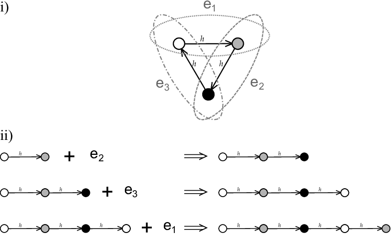
Definition 1
A self-assembly (SA) hypergraph automaton is a tuple where is a hypergraph, called the underlying hypergraph, is the transition function assigning to each hyperedge a transition with , is a pseudo-picture graph with node set called the underlying graph, and is the set of initial hyperedges.
Every hyperedge defines a graph which is the subgraph of induced by . For we call and the incoming active nodes and outgoing active nodes of , respectively. In order for the hypergraph automaton to be well-defined, we require that is connected and that the subgraph of induced by its incoming active nodes is connected, too, for all . If , then is also called an initial graph.
A configuration of the hypergraph automaton is a triple where is a subgrid, is the set of active nodes, and is a function such that for all . The set consists of (possibly multiple) copies of nodes from and the function assigns to each node in its original node in . An edge is a copy of the edge and is a copy of the edge . However, for two nodes and in , if their originals and are connected by a horizontal (or vertical) edge, this does not imply that and are connected by a horizontal (or vertical) edge.
Let be a configuration with and let be a hyperedge with . If there exists a non-empty subset such that forms a graph-isomorphism from the subgraph of induced by to the subgraph of induced by the incoming active nodes , then the hyperedge defines a transition or derivation step
where, informally speaking, the resulting graph consists of joining together the graphs and by identifying every node with the corresponding node . The active nodes in are the active nodes in plus the outgoing active nodes in , see Figure 5. We also say that is the result of gluing the hyperedge to . Formally, the configuration where is constructed as follows. Let be a set containing a copy of each node from except for the incoming active nodes such that . Let and let such that for and for . An edge belongs to if or and ; an edge belongs to if or and . Naturally, for all and . The reflexive and transitive closure of is denoted by and called a derivation.

For we let such that and we call the configuration an initial configuration of . A final configuration is a configuration without active nodes. The graph language accepted by the SA-hypergraph automaton is
Note that contains picture graphs only. The picture language associated to the graph language is the language .
Remark 1
Since we only talk about picture graphs, we can assume that for every hyperedge the underlying graph is a subgrid, or can be removed from the set .
Example 1
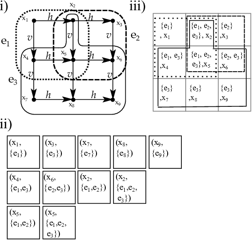
Figure 6 shows an example of a self-assembled coloured pattern and an SA-hypergraph automaton that accepts that pattern. Part i) depicts a coloured self-assembled pattern. Parts ii) and iii) together depict the underlying graph of the SA-hypergraph automaton that constructs the same pattern.

The SA-hypergraph automaton for the example in Figure 5 is defined as follows. The SA-hypergraph automaton is , where
-
,
-
,
-
function is defined such that
-
For each hyperedge in ii), the function describing the active areas where we can glue new hyperedges is defined as to build a horizontal (vertical) chain of nodes that models the top row (left column) of tiles.
The backward edges e.g. , , , and , make it possible to reuse the hyperedges to build a periodic pattern.
For each hyperedge in iii), the function changes the active input nodes (top-left, bottom-left, and top-right) to the new set of active nodes (top-right, bottom-left, and bottom-right), signifying the change of the places where the new hyperedges can be glued.
-
Parts ii) and iii) depict the underlying graphs of the white -shaped top and left border of the pattern, and the white-grey-black part of the pattern respectively.
-
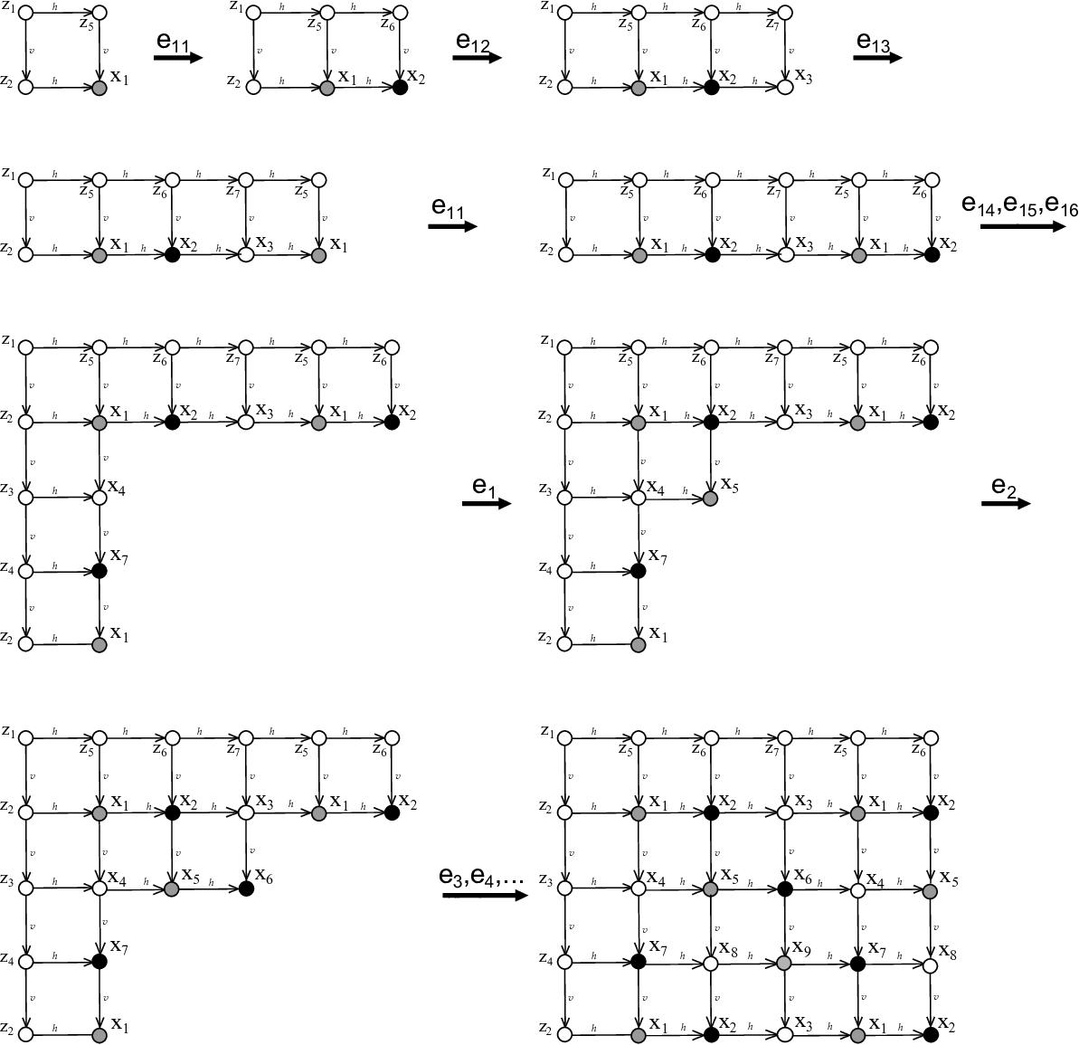
The SA-hypergraph automaton starts from the top-left white tile, corresponding to . Afterwards, the automaton continues the construction with the hyperedges in the top row or the left column. The construction of the white-grey-black part starts after the construction of the white top row and left column. Figure 7 shows an example of possible transitions of the SA-hypergraph automaton .
The concept of hypergraph automata has been introduced by Rozenberg in 1982 [9]. Our definition of SA-hypergraph automata is a variant of the original definition with the following modifications. Firstly, we start from a set of initial graphs whereas the original definition used a single initial graph. For unlabelled graphs both models are capable of accepting the same class of graph languages, as long as one makes an exception for the empty graph. However, for labelled graphs a single initial graph is not sufficient; e. g., if a language of labelled graphs contains one graph where every node is labelled by and one graph where every node is labelled by , then cannot be generated from the same initial graph since and do not have a common non-empty isomorphic subgraph. Secondly, we use final configurations in order to accept only some of the graphs that can be generated by rules from the initial graph. In the original definition, for simplicity, final configurations were omitted and every graph which can be generated from the initial graph belonged to the accepted language. Thirdly, it seemed more convenient to us to use the notion of active nodes rather than active intersections.
4 Some Examples
In this section, we provide three example SA-hypergraph automata and illustrate their relation to self-assembly systems. Our findings, presented in Section 5, do not build upon this section. In all examples, every node in the underlying graph has a distinct colour which, for simplicity, is the same as the identifier of the node.
The following examples shows a SA-hypergraph automaton to accept the pictures in Figure 8 part . This example shows that SA-hypergraph automata can accept a picture language with a simple description. The SA-hypergraph automaton in this example has 8 nodes and 3 hyperedges; the equivalent tile system needs 8 tile types.
Example 2

Example 3 shows a simple picture language containing two 2D-words. The SA-hypergraph automaton uses two overlapping hyperedges with different active inputs and outputs. Therefore, the number of nodes in this SA-hypergraph automaton will be less than the number tiles in a tile assembly system which recognizes the same language. The SA-hypergraph automaton in this example has 4 nodes and 3 hyperedges. An equivalent tile assembly system needs at least 6 tile types.
Example 3

Example 4 shows a language with an infinite number of one dimensional pictures. The SA-hypergraph automaton uses three hyperedges to build the chain, moreover, one more heyperedge is used to make the final configurations. Therefore, the number of nodes in this SA-hypergraph automaton will be less than the number tiles in a tile assembly system which recognizes the same language. The SA-hypergraph automaton in this example has 3 nodes and 4 hyperedges. Whereas an equivalent tile assembly system needs at least 5 tile types (one tile type to start, 3 tile type to build the chain, and one tile type to stop).

5 Hypergraph Automata for Picture Languages
In this section, we establish a strong connection between (WTS-)recognizable picture languages and picture graph languages that can be accepted by SA-hypergraph automata. We prove that the self-assembly of a Wang Tile System can be simulated by an SA-hypergraph automaton, see Theorem 5.1. The main idea is to start the tiling in the top left corner of a tiled picture and then extend the tiled picture downwards and rightwards, just as in Figure 3. Our converse result is slightly weaker: the picture language , associated to the graph language accepted by an SA-hypergraph automaton , is WTS-recognizable if does not contain a strong loop, see Theorem 5.2. The restriction for not to contain a strong loop is a natural assumption as strong loops cannot be used in any derivation that accepts a picture graphs.
Theorem 5.1
For any recognizable picture language there is a SA-hypergraph automaton such that the picture language associated to the graph language is .
Proof
Let be a Wang Tile System that recognizes the picture language , that is . We will slightly modify the WTS such that it fulfils a certain property as described in the following. We define a WTS which recognizes and such that any two copies of a tile in a tiling of must have a row- and a column-distance which is a multiple of . More precisely, for a Wang tiled version of a picture where a tile appears at two positions , we have that divides as well as . This is achieved by using copies of every tile from in ; we let . We will ensure that a tile can only appear at position if and . This property is achieved by defining the glues as , and for we let
Note that a tiled picture of can be converted into a tiled picture of such that the corresponding pictures and coincide by applying the mapping to every tile in . Vice versa, a tiled picture in can be converted into a tiled picture in such that the corresponding pictures and coincide by applying the mapping to every position in .
The modification of will become of importance later in the proof: We need to ensure that for a square of matching tiles , it is not possible to directly attach another copy of any of to this square.
We will define a SA-hypergraph automaton which simulates the assembly of a tiled picture from as described in Figure 3.
Let be a set of nodes such that and let be a bijection. For each node there is a corresponding tile and vice versa. Let , , , be the set of nodes which correspond to tiles on the top, right, bottom, left border of a tiled picture, respectively:
Let be the underlying graph of . The label function is naturally defined as for . For all nodes there is an edge if and only if and either or or ; there is an edge if and only if and either or or . This means if the east edge of a tile can attach to the west edge of tile , then their corresponding nodes and are connected by an -edge . Analogously, if the south edge of a tile can attach to the north edge of tile , then their corresponding nodes and are connected by an -edge .
If or , the language possibly contains pictures with or , respectively, which can be seen as one-dimensional pictures. These pictures have to be treated separately. For now we assume that .
The hyperedges and the transition function define the possible transitions of . In every transition we add exactly one node to the graph of a configuration of . Our naming convention is that is the node which is attached in the derivation step and are incoming active nodes of the hyperedge. Every graph containing only one node which corresponds to a tile in the top left corner is an initial graph. In order to construct a picture graph which represents a picture in we introduce three types of transitions, see Figure 11. The transitions of type I generate the top row of the graph and transitions of type II generate the left column of the graph; both transition types keep every generated node active. Transitions of type III generate the rest of the graph: A node is attached if it has a matching east neighbour (), a matching north neighbour (), and these two nodes are connected by another node (); unless we reach the right or bottom border of the graph the nodes , , and are active after using the transition.

Formally, we define the set of hyperedges , the set of initial edges , the function , and the transition function as following:
Initial graphs: For each , corresponding to a tile in the top left corner, we define a hyperedge with associated nodes and the transition function .
Type I: For all nodes , in the top row, such that , we define a hyperedge with associated nodes and the derivation function .
Type II: For all nodes , in the left column, such that , we define a hyperedge with associated nodes and the derivation function .
Type III: For all nodes and such that and , we define a hyperedge with associated nodes and the derivation function
- 1.
if , (bottom right corner)
- 2.
if , (bottom row)
- 3.
if , (right column)
- 4.
otherwise.
Consider the graph which is induced by the hyperedge . Depending on the type of the hyperedge , the graph contains at least the edges shown in Figure 11. However, by the modification of the Wang tile system above, we ensured that the graph contains exactly those edges shown in Figure 11. Suppose one of the graphs would contain an edge which is not shown in Figure 11, then the tile corresponding to could occur in two positions which are less than three rows and columns apart — a property that was excluded by the modification.
We will show that . Firstly, consider an array of tiles from which is the Wang-tiled version of the picture . We will show that the SA-hypergraph automaton accepts a picture graph such that . We assume to be embedded in such that the nodes cover the axis-parallel rectangle spanned by the points and , every -edge points downwards, and every -edge points rightwards; recall that our coordinates represent the rows and columns of a matrix. The derivation leading to the final configuration simulates the assembly of tiles which form as shown in Figure 3. The north and west edges of the tile in the top left corner of are labelled by , and therefore, the node corresponding to forms an initial graph . The adjacent edges of two neighbouring tiles in are labelled by the same colour. Suppose is the west neighbour of , then and both tiles belong to the same row, implying that and . Therefore, their corresponding nodes in are connected by an -edge . Analogously, if is the north neighbour of , then . Next, we see that the hyperedges of type I and type II can be used in order to create the top row and left column of the graph , respectively. Furthermore, the hyperedges of type III can be used in order to create all the remaining nodes of . We conclude that is a derivation in and we will prove that has to be a final configuration with . Observe, that hyperedges of types I and II leave all the nodes active while hyperedges of type III deactivate at least the top left node in the hyperedge. Thus, all nodes except for those in the bottom row and in the right column will be deactivated in the configuration . Furthermore, in order to create the bottom row and right column hyperedges of type III.2 and III.3 are used, respectively, and one rule of type III.1 is used in order to create the bottom-right node of . It is easy to see that the derivation function is designed such that all nodes will be deactivated in the configuration and, therefore, accepts .
Now, let be a graph which is generated by . Let be accepted by the derivation
where is an initial configuration with and is a final configuration. Let be the node set of the graph . Note that for any the function is the restriction of by , that is . In order to avoid confusion, nodes in the graph are consistently denoted by and nodes in the graph are consistently denoted by ; the nodes may have subscripts.
Let the nodes in the graphs be embedded in such that all -edges point rightwards and all -edges point downwards; just like we did above. The creation of graph starts with the initial graph which contains only one node . Let lie on position in all of the graphs . The graph can be extended rightwards by using hyperedges of type I and downwards by hyperedges of type II. Since none of the hyperedges attach a new node upwards or leftwards of an existing node in in order to obtain , the node lies in the top row and in the left column of . By the definition of type I and II hyperedges, for every node in the top row (resp., left column) of we have (resp., ). By using hyperedges of type III the area spanned by the top row and left column can be filled with nodes. It is easy to see that for all graphs we have that if a node lies on position , then for all a node lies on position . Furthermore, if , then the node on position has an outgoing -edge, and if , then the node on position has an outgoing -edge. In other words, in the axis-parallel rectangle spanned by the points and all nodes are connected by edges with all direct neighbours (nodes which have an Euclidean distance of ).
In the final configuration there is no active node. Thus, the last node which is added to the graph in order to obtain is a node such that , as all other derivation rules will leave some nodes active. Next, let us consider the nodes which belong to the same row and column as does. Note that if two nodes and in are connected by an edge, then the corresponding nodes and in are connected by an edge, too; more precisely, if , then , and if , then . Since a node in (resp., ) only is connected by -edges (resp., -edges) in to other nodes from (resp., ), we see that for every node in the row of (resp., column of ) we have (resp., ). A node (resp., ) does not have any outgoing -edges (resp., -edges) as the south edge (resp., east edge) of is labelled by . We conclude that sits in the bottom row and right column of the graph and, by the observations made above, this implies that is a picture graph.
We claim that the picture which corresponds to the graph can be generated by the assembly given by the embedding of nodes in and the function . Clearly, for every node on position in we have that , therefore, the pictures and coincide. Next, we prove that is a tiled picture in the Wang tile system . Recall, that all nodes on the top, right, bottom, and left border of correspond to tiles in , , , and , respectively, and therefore, is well-bordered. Let and be two neighbouring tiles in which lie on positions and , respectively. Let and be the nodes in which lie on the positions and , respectively. Note that and . Since is a picture graph, and . The edge set was build to ensure that . We conclude that all adjacent east-west edges in have matching colours. By symmetric arguments, we also conclude that all adjacent north-south edges in have matching colours. Therefore, is a tiled picture in and .
Finally, let us consider the case when . We can add a component to the SA-hypergraph automaton which works similar to a non-deterministic finite automaton and where every hyperedge induces an graph of type I in Figure 11. The initial graphs are given by all nodes from . For all nodes with we define a hyperedge such that . The derivation function is given as if , and otherwise. Obviously, this attachment to the hypergraph accepts all graphs which correspond to pictures with . The case when can be covered analogously. ∎
Next, we prove that a picture language , associated to the graph language , is WTS-recognizable if does not contain a strong loop.
Let be an SA-hypergrph automaton. A series of hyperedges from is a (derivation) loop if and where for . Loops in an SA-hypergraph automaton are a prerequisite for using a hyperedge several times in one derivation. Therefore, an SA-hypergraph automaton without any loops can only accept a finite graph language. Let be the graph induced by , let be a node in , and let be set overlapping incoming/outgoing active nodes of and . There is a path in the underlying graph of from to which only visits the subgraphs , in the given order, and passes through at least one node of each (the path may use incoming and outgoing edges). The loop is a strong loop if, on this path, the number of incoming horizontal edges equals the number of outgoing horizontal edges and the number of incoming vertical edges equals the number of outgoing vertical edges. In other words, when starting from a configuration and successively gluing the hyperedges from to , then the subgraph added by the hyperedge and the subgraph added by the hyperedge fully overlap when naturally embedded in . Note that, by Remark 1, all graphs are subgrids which implies that the choice of the path from to does not matter in this definition.
Theorem 5.2
Let be a SA-hypergraph automaton without any strong loops. The picture language , associated to the graph language , is WTS-recognizable (Wang tile system recognizable).
Proof
Let and let . We may assume that if and only if . Therefore, none of the initial hyperedges can be used in a transition. This assumption is justified by the fact that we can duplicate all hyperedges in such that one copy can be used in a transition but does not belong to and the other copy which belongs to cannot be used in a transition. Furthermore, any hyperedge without incoming active nodes which does not belong to is useless and can be removed from .
For a node we define the list of related hyperedges to , . Let be a node and . We call a hyperedge a generator of if with . Note that if , then must be a generator. We call a hyperedge a consumer of if with . The pair is a tile candidate if contains exactly one generator and exactly one consumer ; furthermore, if , we require that . Note that if , then for all with , we have that unless is the generator and unless is the consumer. The tile candidate describes the attachment of a copy of the node to the output graph by the generator; afterwards, is used as active node by all hyperedges in ; finally, is deactivated by the consumer. Let be the node-induced subgraph of by . If is not a subgrid (a subgraph of some picture graph), we remove from the set of tile candidates. Let denote the set of all remaining tile candidates.
The Wang tile system which recognizes is constructed based on the list . In order to recognize the picture language associated to , we have to define the attachments of tile candidates. We use unordered pairs of tile candidates for the colours on the edges. For a tile candidate we define the set of labelled Wang tiles
where is the label and , , , are sets of colours which are defined below. The set of all tiles is the union .
For , we let and if and only if
- 1.
,
- 2.
,
- 3.
, and
- 4.
or for or for .
For , we let and if and only if and conditions 2 to 4 are satisfied. For , we let if does not have an incoming vertical edges in the graph . By symmetric condition we let , , or .
Now, consider an -picture graph . We will show that there is a tiled version of picture which uses tiles from and, therefore, is recognized by . Let be accepted by the derivation
where is an initial configuration (that is ) and is a final configuration. Let be the hyperedge and be the active nodes which are used in the transition . Let for . Recall that, by definition, is a full subgraph of and, by induction, every graph is a full subgraph of . Being an -picture graph, the nodes in can be naturally embedded in by the function .
Consider one node and its original in . We assign to a list of hyperedges such that if or belongs to but not . We intend to use a tile from for the pixel representing in the tiled picture . Observe that contains a consumer as is not active in the final configuration and cannot contain two consumers because a node can only be deactivated once. In addition, the hyperedge such that belongs to but not is the single generator in . Since is isomorphic to a subgraph of , we conclude that is indeed a tile candidate. If does not have an outgoing horizontal edge, then the node in the graph cannot have an outgoing horizontal edge either and, therefore, . Symmetric arguments apply if does not have an incoming horizontal, outgoing vertical, or incoming vertical edge.
Next, consider two nodes which are connected by an edge and, by symmetry, assume is a horizontal edge. Let , be their originals and let be the set of hyperedges associated to , respectively. We will show that is a colour in as well as in . Thus, we can choose tiles from and for the positions and in , respectively. Clearly, the choice of the tiles also depends on the other neighbours of and . We have to show that conditions 1 to 5, above, are satisfied. The first condition is satisfied by assumption. By contradiction, suppose the second condition is not satisfied. There is ; thus, in the -th step of the derivation we use the hyperedge that presupposes or generates an edge in where but . This would imply that has two incoming horizontal edges whence is not a picture graph. The third condition is satisfied by symmetric arguments. The edge in can only be created in a step where or is added to the graph . Thus, and either have the same generator in and , or is in the active nodes when is generated, or is in the active nodes when is generated. In all cases condition 4 is satisfied.
We conclude that a tiled picture such that and can be generated by using tiles from and, therefore, .
Consider a picture and let be the tiled version of , using tiles from .
We start by introducing the concept of masks which can be seen as connected subpictures of the tiled picture that represent the nodes in one hyperedge. A mask is a matrix of tiles from , such that either or for all . In addition, we require that the non-empty entries in are connected; that is, for every pair of tiles there exists a sequence of tiles in such that , , , and , must be adjacent for all .
Let be an hyperedge and let be the graph induced by this hyperedge. By Remark 1, we assume that is a subgrid. We say is mapped to a mask if there is a injective function which satisfies: belongs to if and only if is in the domain of ; for all nodes there is an edge (resp., ) if and only if is in north (resp., west) neighbour of . Whenever we use this mapping, we will ensure that for all the tile belongs to for some .
Consider a tile and a hyperedge . We define the mask such that the graph can be mapped by function to and . We say that is the hyperedge related to the mask . Let be a tile that is adjacent to and let . For simplicity we only consider the case when is the east neighbour of ; i.e., . We will show that if is non-empty in , then . Since is the east neighbour of conditions 1 to 4, above, apply. As is non-empty in , there exists a horizontal edge in . Furthermore, from conditions 1 and 4 it follows that is a horizontal edge in the graph induced by the generator . As both graphs and are subgraphs of the subgrid , we see that the edges and coincide, thus, . We conclude and . By condition 3, . Because the hyperedge induces a connected graph, we can infer that for all non-empty , we find . Note that this also implies that .
We define the set of masks which are induced by hyperedges in the above manner. Intuitively, every mask in represents one transition in the derivation of a picture graph which represents the picture . In order to use a transition defined by a mask, we need to guarantee that all of its input areas exist and are active. We will order the set accordingly. Let us define the relation such that if the transition represented by has to be used before the transition represented by . Let and be two distinct masks in . The pair is in if there exists such that , and where or where . The pair can be seen as directed graph . First, we show that the graph does not contain any loops, afterwards, a topological sort of this graph is used to order the transitions represented by the masks.
When two or masks overlap on a tile (have a common non-empty entry), regarding the construction of tile candidates, we know that the related hyperedge of exactly one of these masks is the generator of the input area of the other hyperedges. Hence, these masks are connected in the graph . By contradiction, assume that is a non-trivial loop in (i.e., for every and ). However, the sequence of related hyperedges to this sequence of mask is a strong loop in the SA-hypergraph automaton which was excluded by assumption. Moreover, since two tiles with different generators cannot connect without satisfying conditions 4, the graph must be connected. Therefore, graph can be topologically sorted. Sorting of the hyperedges guaranteed that the active input nodes of one hyperedge are generated before the gluing of the hyperedge.
By contraction, assume that graph has two distinct nodes and without any input edges. Let be the first node in the topological order such that paths and exist in . As is chosen minimal, these paths do not share any node other than . Recall that all incoming active nodes of a hyperedge are connected. Considering that two nodes cannot connect to each other unless they are in the same hyperedge or they have glued to each other, we have a contradiction as cannot be the first common node on both paths. We conclude that graph has only one node without input.
Now, let be the topological sort of by the relation . We define such that if ; otherwise, . We will show that a graph can be generated by a derivation
such that the graph can be mapped to the mask ; this implies that can be mapped to . Let be the hyperedge related to the mask . The graph is an initial graph because has no incoming edges in and, therefore, the derivation function of is ; thus, where and is an initial configuration. In derivation step we use the hyperedge . By induction, we can assume that can be mapped to by a function . There is only one way to glue the hyperedge to such that resulting graph can be mapped to . We have to prove that all incoming active nodes of exist and are active in . Let be an incoming active node which is represented by the tile . The definition of ensures that the mask representing the generator of in has already been used and that the mask representing the consumer of in has not yet been used. Finally, every tile candidate has a consumer which means that there are no active nodes in the final configuration . As result, the picture , generated by the suggested tiling system, is in . ∎
6 Conclusion
We introduced SA hypergraph automata, a language/automata theoretic model for patterned self-assembly systems. SA hypergraph automata accept all recognizable picture languages but, unlike other models, (e.g. Wang Tile Automata) SA-hypergraph automata do not rely on an a priori given scanning strategy of a picture. This property makes the SA hypergraph automata better suited to model DNA-tile-based self-assembly systems.
SA-hypergraph automata provide a natural automata-theoretic model for patterned self-assemblies that will enable us to analyse self-assembly in an automata-theoretic framework. This framework lends itself easily to, e.g., descriptional and computational complexity analysis, and such studies may ultimately lead to classifications and hierarchies of patterned self-assembly systems based on the properties of their corresponding SA-hypergraph automata. An additional feature is that each SA-hypergraph automaton accepts an entire class of “supertiles” as opposed to a singleton set, which may also be of interest for some applications or analyses.
References
- [1] M. Anselmo, D. Giammarresi, and M. Madonia. Tiling automaton: A computational model for recognizable two-dimensional languages. In CIAA, pages 290–302. 2007.
- [2] R. D. Barish, R. Schulman, P. W. K. Rothemund, and E. Winfree. An information-bearing seed for nucleating algorithmic self-assembly. Proceedings of the National Academy of Sciences, 2009.
- [3] M. Blum and C. Hewitt. Automata on a 2-dimensional tape. In SWAT (FOCS), pages 155–160, 1967.
- [4] E. Czeizler and A. Popa. Synthesizing minimal tile sets for complex patterns in the framework of patterned DNA self-assembly. In DNA Computing and Molecular Programming, volume 7433 of Lecture Notes in Computer Science, pages 58–72. Springer Berlin / Heidelberg, 2012.
- [5] L. de Prophetis and S. Varricchio. Recognizability of rectangular pictures by Wang systems. Journal of Automata, Languages and Combinatorics, 2(4):269, 1997.
- [6] D. Giammarresi and A. Restivo. Two-dimensional languages, pages 215–267. Springer-Verlag, 1997.
- [7] M. Göös and P. Orponen. Synthesizing minimal tile sets for patterned DNA self-assembly. In DNA, pages 71–82, 2010.
- [8] K. Inoue and A. Nakamura. Some properties of two-dimensional on-line tessellation acceptors. Inf. Sci., 13(2):95–121, 1977.
- [9] D. Janssens and G. Rozenberg. Hypergraph systems generating graph languages. In Graph-Grammars and Their Application to Computer Science, pages 172–185, 1982.
- [10] T. Lempiäinen, E. Czeizler, and P. Orponen. Synthesizing small and reliable tile sets for patterned DNA self-assembly. In DNA, pages 145–159, 2011.
- [11] V. Lonati and M. Pradella. Picture recognizability with automata based on Wang tiles. In SOFSEM, pages 576–587, 2010.
- [12] V. Lonati and M. Pradella. Strategies to scan pictures with automata based on Wang tiles. RAIRO - Theor. Inf. and Applic., 45(1):163–180, 2011.
- [13] X. Ma and F. Lombardi. Synthesis of tile sets for DNA self-assembly. IEEE Trans. on CAD of Integrated Circuits and Systems, 27(5):963–967, 2008.
- [14] P. W. K. Rothemund, N. Papadakis, and E. Winfree. Algorithmic self-assembly of DNA Sierpinski triangles. PLoS Biology, page 2004.
- [15] E. Winfree. Algorithmic self-assembly of DNA. PhD thesis, 1998.