Four-Dimensional Quantum Hall Effect in a Two-Dimensional Quasicrystal

The uprising field of topological phases of matter deals with systems of arbitrary dimension [1, 2]. In this paradigm, each energy gap of a system is attributed an index, which is robust to continuous deformations. A nontrivial index is usually associated with interesting boundary phenomena, quantized response, and exotic quasiparticles. While nontrivial topological phases appear in any dimension [3, 4], the physical manifestations are limited to 1D [5, 6], 2D [7, 8] and 3D [9].

An example of an intriguing topological phase, which is seemingly out of reach, is the 4D generalization of the 2D integer quantum Hall effect (IQHE). In 2D, a uniform magnetic field creates Landau levels that are characterized by the $1^{\textrm{st}}$ Chern number—the topological index that corresponds to the quantized Hall conductance [10, 11]. In 4D, a uniform SU(2) Yang-Mills field results in generalized Landau levels [12, 13]. These levels are characterized by the $2^{\textrm{nd}}$ Chern number – a topological index which corresponds to a quantized non-linear response [13, 14]. Both the 2D and 4D IQHEs exhibit a variety of exotic strongly correlated phases when interactions are included [13, 15]. Hence, the 4D IQHE, as well as lattice models with non-vanishing $2^{\textrm{nd}}$ Chern numbers, constantly attract theoretical attention [14, 16], such as the recently found rich metal-insulator phase diagram [17].

The physical properties of quasicrystals (QCs) – non-periodic structures with long-range order – can oftentimes be derived from periodic models of higher dimensions [18, 19]. Using a novel dimensional extension, it was recently shown that 1D QCs exhibit topological properties of the 2D IQHE [20]. The bulk energy spectrum of these 1D QCs is gapped, and each gap is associated with a nontrivial $1^{\textrm{st}}$ Chern number. This association relies on the fact that the long-range order harbors an additional degree-of-freedom in the form of a shift of the quasiperiodic order. Accordingly, boundary states traverse the gaps as a function of this shift. This property was observed in photonic QCs, and was utilized for an adiabatic pump of light [20]. Moreover, upon a deformation between QCs with different $1^{\textrm{st}}$ Chern numbers, the expected phase transition was experimentally observed [21]. Generalizations to other 1D symmetry classes, physical implementations, and QCs were discussed [22, 23, 24, 25].

In this Letter, we take a major step further, and present a 2D quasiperiodic model that exhibits topological properties of the 4D IQHE. Each gap in its energy spectrum is characterized by a nontrivial $2^{\textrm{nd}}$ Chern number, which implies quantum phase transitions between topologically distinct models. Furthermore, scanning of the shift parameters is accompanied by (i) quantized charge pumping with an underlying 4D symmetry, and (ii) gap-traversing edge states with protected level crossings. Generalizations to other models and 2D QCs are discussed. We propose two experiments to measure the $2^{\textrm{nd}}$ Chern number via charge pumping, and, thus, make 4D physics experimentally accessible.

We study a 2D tight-binding model of particles that hop on a square lattice in the presence of a modulated on-site potential

Here $\sigma=\pm$ is an internal degree of freedom such as spin-$\frac{1}{2}$, photonic polarization, or atomic orbital, $c_{x,y,\sigma}$ is the single-particle annihilation operator of a particle at site $(x,y)$ in state $\sigma$; $t_{x},t_{y}$ are the hopping amplitudes in the $x$ and $y$ directions; and $\lambda_{x},\lambda_{y}$ are the amplitudes of the on-site potentials, which are modulated along $x$ and $y$ with modulation frequencies $b_{x},b_{y}$, respectively [cf. Fig. 1(a)]. Last, the Hamiltonian depends on two shift parameters $\phi_{x}$ and $\phi_{y}$. We assume the modulation frequencies $b_{x}$ and $b_{y}$ to be irrational, which makes the on-site modulations incommensurate with the lattice, and the model becomes quasiperiodic.

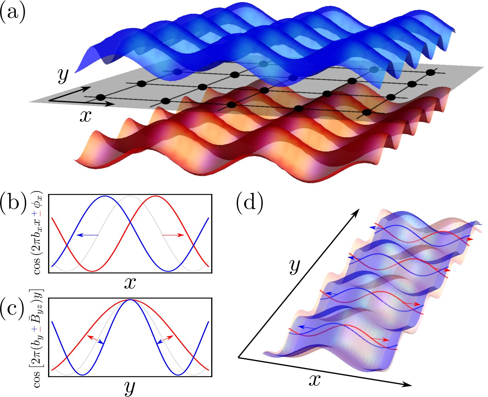
The spectrum of $H$ is gapped, and therefore, may exhibit nontrivial topological indices. Conventionally, the only apparent topological index that can be associated with $H$ is the $1^{\textrm{st}}$ Chern number [3, 4]. However, since $H(\phi_{x}=\phi_{y}=0)$ is time-reversal symmetric, its $1^{\textrm{st}}$ Chern number vanishes, and $H$ is seemingly trivial.

Strikingly, $H$ is attributed a nontrivial $2^{\textrm{nd}}$ Chern number, which, by definition, characterizes 4D systems. In order to obtain this result, let us consider $H$ on a toroidal geometry [26]. We introduce twisted boundary conditions along the $x$ and $y$ directions, parameterized by $\theta_{x}$ and $\theta_{y}$, respectively. For a given gap and given $\phi_{\mu}\equiv(\phi_{x},\phi_{y},\theta_{x},\theta_{y})$, we denote by $P(\phi_{\mu})$ the projection matrix on all the eigenstates of $H(\phi_{\mu})$ with energies below this gap. We can now define,

where $\epsilon_{\alpha\beta\gamma\delta}$ is the antisymmetric tensor of rank-$4$.

Formally, the $2^{\textrm{nd}}$ Chern number is defined by $\mathcal{V}=\int d^{4}\phi_{\mu}\;\mathcal{C}(\phi_{\mu})$ [27]. By its definition, $\mathcal{V}$ characterizes a 4D family of Hamiltonians composed of all $H(\phi_{\mu})$ with all possible values of $\phi_{\mu}$; i.e. $\phi_{x}$ and $\phi_{y}$ act as two additional effective dimensions. The main result of this Letter is that even for a given $\phi_{\mu}$, the gaps of $H(\phi_{\mu})$ can be associated with a nontrivial integer $2^{\textrm{nd}}$ Chern number,

in the thermodynamic limit. Below, we justify Eq. (3) by showing that, for our model, $\mathcal{C}(\phi_{\mu})$ is essentially independent of $\phi_{\mu}$, and thus the integration over the four parameters is redundant.

Beforehand, we present the physical implications of the nontrivial $\mathcal{V}$. To do so, we apply to $H$ the procedure of dimensional extension that was introduced in Refs. [20, 23]. In this procedure, we interpret $\phi_{x}$ and $\phi_{y}$ as momenta along two fictitious perpendicular coordinates $w$ and $z$, respectively. Now, the Hamiltonian $H(\phi_{x},\phi_{y})$ is a single Fourier component of some ancestor 4D Hamiltonian $\mathcal{H}$. By making the inverse Fourier transform, we obtain a Hamiltonian describing spin-$\frac{1}{2}$ particles hopping on a 4D hyper-cubic lattice

where $\mathbf{c}_{\mathbf{x}}=(c_{\mathbf{x},+},c_{\mathbf{x},-})$ annihilates a spin-$\frac{1}{2}$ particle at site $\mathbf{x}=(x,y,z,w)$, $\hat{\mu}$ is summed over the unit vectors $\hat{x},\hat{y},\hat{z}$ and $\hat{w}$, which connect nearest neighbors, and $t_{\hat{\mu}}=(t_{x},t_{y},\lambda_{x}/2,\lambda_{y}/2)$. These particles are coupled to a Yang-Mills gauge field $a_{\hat{\mu}}(\mathbf{x})=(b_{y}y\hat{z}+b_{x}x\hat{w})\sigma_{3}$. This vector potential describes a spin-polarized uniform SU(2) field. Such a field in known to generate a 4D IQHE with a nontrivial $\mathcal{V}$ [12, 13]. Notably, $\mathcal{H}$ is defined on a planar geometry in a Landau gauge, whereas previous analyses treated a spherical geometry in a symmetric gauge.

Similar to the 2D IQHE, $\mathcal{V}$ has a physical manifestation in the form of a response function. Here the response is quantized but non-linear: $j_{\alpha}=\mathcal{V}\frac{e^{2}}{h\Phi_{0}}\epsilon_{\alpha\beta\gamma\delta}B_{\beta\gamma}E_{\delta}$ [14], where $j_{\alpha}$ denotes the current density along the $\alpha$ direction, $\Phi_{0}$ is the flux quantum, $E_{\delta}$ is an electric field along the $\delta$ direction, and $B_{\beta\gamma}$ is a magnetic field in the $\beta\gamma$ plane.

A direct observation of this response requires a 4D system. However, we can develop an analogue of Laughlin’s pumping, which is manifested in the 2D model. Let us consider the following two cases: $j_{x}=\mathcal{V}\frac{e^{2}}{h\Phi_{0}}B_{yz}E_{w}$ and $j_{x}=\mathcal{V}\frac{e^{2}}{h\Phi_{0}}B_{wy}E_{z}$. Recall that the electric fields can be generated by time-dependent Aharonov-Bohm fluxes, $E_{w}=\frac{1}{caN_{w}}\partial_{t}\Phi_{w}(t)$ and $E_{z}=\frac{1}{caN_{z}}\partial_{t}\Phi_{z}(t)$, where $a$ is the lattice spacing, and $N_{w}$ and $N_{z}$ are the number of lattice sites along the $w$ and $z$ directions, respectively. Expressing $B_{yz}$ and $B_{wy}$ in $\mathcal{H}$ in Landau gauge, and performing dimensional reduction, these fields enter the 2D model, $H$, through modified on-site terms,

where $\phi_{x}(t)=\frac{2\pi}{N_{w}\Phi_{0}}\Phi_{w}(t)$ and $\phi_{y}(t)=\frac{2\pi}{N_{z}\Phi_{0}}\Phi_{z}(t)$, and $\bar{B}_{wy}=B_{wy}a^{2}/\Phi_{0}$ and $\bar{B}_{yz}=B_{yz}a^{2}/\Phi_{0}$ denote the corresponding flux quanta per plaquette. Figures 1(b)-(d) illustrate the effects of these modifications. By fixing the chemical potential within a gap with a given $\mathcal{V}$, an adiabatic scan of $\phi_{x}$ or of $\phi_{y}$ from $0$ to $2\pi$ pumps charge along the $x$ direction, such that

respectively, where $N_{y}$ is the number of lattice sites along the $y$ direction.

We can now propose experiments that measure $\mathcal{V}$ using Eq. (6). Take a 2D slab of our model, and connect metal leads to the edges of the $x$ coordinate. Let us assume that the chemical potential of both the system and the leads is placed in some gap of $H$. Then, one should measure the charge-flow during the scan of $\phi_{x}$ from $0$ to $2\pi$ for different values of $\bar{B}_{yz}$ [28]. According to Eq. (6a), we expect that $\mathcal{V}=\frac{1}{eL_{y}}\partial Q_{x}/\partial\bar{B}_{yz}$. Similarly, according to Eq. (6b), during the scan of $\phi_{y}$ while varying $\bar{B}_{wy}$, charge flows and $\mathcal{V}=\frac{1}{eL_{y}}\partial Q_{x}/\partial\bar{B}_{wy}$. Remarkably, due to the 4D origin of our model, the measured $\mathcal{V}$ would be the same in both experiments. A similar experiment can be conducted in a photonic system [29].

We have just seen that upon a scan of $\phi_{x}$, charge may flow in the $x$ direction. Consequently, for an open geometry, in order to accommodate this charge transfer, edge states must appear and traverse the gaps as a function of $\phi_{x}$. These states appear for infinitesimally small $\bar{B}_{yz}$, and hence appear also for $\bar{B}_{yz}=0$. Figure 2 depicts the numerically obtained energy spectrum of $H$ as a function of $\phi_{x}$, for an open $x$ coordinate, a periodic $y$ coordinate, $t_{x}=t_{y}=1$, $\lambda_{x}=\lambda_{y}=1.8$, $N_{x}=N_{y}=34$, $b_{x}=(1+\sqrt{5})/2$ and $b_{y}=55/34\approx(1+\sqrt{5})/2$ [26]. The spectrum is invariant with respect to $\phi_{y}$, and is depicted for $\phi_{y}=0$. As a function of $\phi_{x}$, the spectrum has flat bands and gap-traversing bands. The flat bands correspond to bulk states, whereas the gap-traversing ones to edge state (see insets). The edge states are divided into four types: $\sigma=+$ and $\sigma=-$ (blue and red), which are localized at either the left or right edge (opposite slopes). These edge states are a signature of the nontrivial $\mathcal{V}$ of our model. They can be measured in a way similar to the experiments performed in 1D photonic QCs [20, 29].

Naively, opposite-$\sigma$ modes that reside on the same edge can be gapped out by introducing $\sigma$-mixing terms. However, this is not the case, and the edge modes and their crossings are topologically protected. In order to establish this protection, we decompose $H$ into its $\sigma$ and spatial constituents. The Hamiltonian $H$ is a sum of two $\sigma$ components, where each $\sigma$ component is subject to two decoupled 1D Harper models along the $x$ and $y$ directions. Both $\sigma$ components experience the same modulation frequencies, $b_{x}$ and $b_{y}$, but couple to the shift parameters, $\phi_{x}$ and $\phi_{y}$, with an opposite sign. Therefore, each eigenstate of $H(\phi_{x},\phi_{y})$ is a product of eigenstates of the Harper models in the $x$ and $y$ directions and an eigenstate of $\sigma$.

Recall that each gap of the Harper model is associated with a nontrivial $1^{\textrm{st}}$ Chern number, which corresponds to the number of boundary states that traverse the gap as a function of $\phi$ [10, 11, 20]. Accordingly, each band of the Harper models in the $x$ and $y$ directions is associated with some $\sigma$-dependent $1^{\textrm{st}}$ Chern number, $\nu_{r_{x},\sigma}$ and $\nu_{r_{y},\sigma}$, where $r_{x}$ and $r_{y}$ denote the corresponding bands, respectively [30]. In Fig. 2, the bands that traverse the gaps as a function of $\phi_{x}$ are composed of products of bulk bands in the $y$ direction and boundary states in the $x$ direction. Notably, due to the opposite coupling of $\sigma$ to $\phi_{x}$ and $\phi_{y}$, $\nu_{r_{x},-}=-\nu_{r_{x},+}$ and $\nu_{r_{y},-}=-\nu_{r_{y},+}$. Therefore, the gaps are traversed by the same number of $\sigma=\pm$ bands, but with opposite slopes. Since opposite-$\sigma$ bands are associated with opposite $1^{\textrm{st}}$ Chern numbers, they cannot be gapped out by $\sigma$-mixing terms, even if they cross at some value of $\phi_{x}$. Otherwise, $\nu_{r_{y},\sigma}$ would change continuously as a function of $\phi_{x}$ between $\nu_{r_{y},+}$ and $\nu_{r_{y},-}$. The level crossing is therefore protected.

The described edge phenomena accounts for the charge pumping described above. When $\phi_{x}$ or $\phi_{y}$ are scanned, opposite-$\sigma$ states, which have opposite $1^{\textrm{st}}$ Chern numbers, flow in opposite directions. In the absence of $\bar{B}_{yz}$ and $\bar{B}_{wy}$, the two charge currents cancel. Applying $\bar{B}_{yz}$ or $\bar{B}_{wy}$ causes a difference between the densities of the $\sigma$ states, and thus a net charge is pumped [14, 31]. Remarkably, for a spin-$\frac{1}{2}$ realization, our model can serve as a spin pump across the sample, since for recursive scans of $\phi_{x}$, macroscopic spins accumulate at the boundaries, even for vanishing $\bar{B}_{yz}$ and $\bar{B}_{wy}$.

We turn, now, to establish Eq. (3). Let us evoke the definition of the $1^{\textrm{st}}$ Chern number of a band of the Harper model in the $x$ direction with a given $\sigma$, $\nu_{r_{x},\sigma}=\int d\phi_{x}d\theta_{x}\;C_{r_{x},\sigma}(\phi_{x},\theta_{x})$, where $C_{r_{x},\sigma}(\phi_{x},\theta_{x})=\frac{1}{2\pi i}\textrm{Tr}(P_{r_{x},\sigma}[\partial_{\phi_{x}}P_{r_{x},\sigma},\partial_{\theta_{x}}P_{r_{x},\sigma}])$, and $P_{r_{x},\sigma}(\phi_{x},\theta_{x})$ is the projection matrix on the eigenstates of the $r_{x}$th band [27]. A similar definition applies for $\nu_{r_{y},\sigma}$. Let us denote by $\epsilon_{n}(\phi)$ the eigenenergies of the Harper model. The decomposition of $H$ into $x$ and $y$ constituents makes its energy spectrum a Minkowski sum, $E_{n_{x},n_{y},\sigma}(\phi_{x},\phi_{y})=\epsilon_{n_{x}}(\sigma\phi_{x})+\epsilon_{n_{y}}(\sigma\phi_{y})$. Accordingly, the states below each gap of $E_{n_{x},n_{y},\sigma}$ can be decomposed into a sum over pairs of bands in the 1D spectra, $r_{x}$ and $r_{y}$, such that $\epsilon_{r_{x}}+\epsilon_{r_{y}}<\mu$, where $\mu$ is the energy in the middle of the gap. Using the fact that the eigenfunctions of $H$ are a product of the 1D eigenfunctions, we obtain [29]

In a previous work [20], we have shown that, in the thermodynamic limit, $C_{r,\sigma}(\phi,\theta)$ becomes independent of $\phi$ and $\theta$. Hence $\nu_{r,\sigma}=(2\pi)^{2}C_{r,\sigma}(\phi,\theta)$. This, combined with Eq. (6), immediately implies Eq. (3) [29].

Until now, our analysis used the decomposition of $H$ into $\sigma$, $x$ and $y$ components. In fact, any SU(2)$\times$U(1) gauge transformation in the 4D Hamiltonian $\mathcal{H}$ that respects Landau gauge keeps the system unchanged. After the dimensional reduction to 2D, such a transformation becomes a general local transformation that may mix $x$, $y$, and $\sigma$, but keeps $\mathcal{V}$ unchanged. More generally, any unitary transformation of the 2D Hamiltonian that does not depend on $\phi_{\mu}$ keeps $\mathcal{C}(\phi_{\mu})$ independent of $\phi_{\mu}$. We also show that the symmetry of $H$ to spin flip is unnecessary [29]. Additionally, in the presence of uncorrelated disorder that does not close the bulk gap, $\mathcal{V}$ remains the same, similar to the 1D case [20].

The predicted $2^{\textrm{nd}}$ Chern number is not limited to a 2D model composed of two Harper models. One can consider (i) placing the cosine modulations in the hopping terms, rather than in the on-site terms (off-diagonal Harper), and (ii) replacing each of the cosine modulations with a Fibonacci-like modulation. Combining (i) and (ii) leads to a well-known 2D QC [32]. In 1D, all these variants were shown to be topologically equivalent to the Harper model, namely they have the same distribution of $1^{\textrm{st}}$ Chern numbers [23]. Therefore, the gaps in such 2D QCs variants will have nontrivial $\mathcal{V}$. Note, also, that similar models that do not depend on $\sigma$ can have gaps with nontrivial $\mathcal{V}$ with accompanying bulk response and edge phenomena [29].

To conclude, in this Letter we have presented a novel 2D quasiperiodic model that is associated with the same topological index as the 4D IQHE – the $2^{\textrm{nd}}$ Chern number. Correspondingly, our model exhibits an elaborate edge phenomena and a quantized charge-pump. We propose experiments in which charge is pumped through the system following modifications of the quasiperiodic modulation. Interestingly, while these modifications differ considerably, they lead to the same pumped charge. This equivalence may seem baffling from a 2D perspective, but follows from the symmetry of the non-linear response in 4D. Recent progress in controlling and engineering systems, such as optical lattices [33], photonic crystals [34, 35], and molecule assembly on metal surfaces [36], makes our 2D model seem experimentally feasible. Moreover, interactions in such systems may lead to fractional quasicrystalline phases which are descendants of the exotic 4D fractional quantum Hall effect [13]. Thus, our model serves as a porthole by which to access 4D physics.

We thank E. Berg and Y. Lahini for fruitful discussions. We acknowledge the Minerva Foundation of the DFG, the US-Israel BSF, and the Swiss National Foundation for financial support. Authors’ names appear in alphabetical order.

SUPPLEMENTAL MATERIAL

References

- [1] M. Z. Hasan and C. L. Kane, Rev. Mod. Phys. 82, 3045 (2010).
- [2] X.-L. Qi and S.-C. Zhang, Rev. Mod. Phys. 83, 1057 (2011).
- [3] R. Shinsei, A. P. Schnyder, A. Furusaki, and A. W. W. Ludwig, New J. Phys. 12, 065010 (2010).
- [4] A. Kitaev, AIP Conf. Proc. 1134, 22 (2009).
- [5] V. Mourik, K. Zuo, S. M. Frolov, S. R. Plissard, E. P. A. M. Bakkers, and L. P. Kouwenhoven, Science 336, 1003 (2012).
- [6] A. Das, Y. Ronen, Y. Most, Y. Oreg, M. Heiblum, and H. Shtrikman, Nature Physics 8, 887 (2012).
- [7] K. v. Klitzing, G. Dorda, and M. Pepper, Phys. Rev. Lett. 45, 494 (1980).
- [8] M. König, S. Wiedmann, C. Brüne, A. Roth, H. Buhmann, L. W. Molenkamp, X.-L. Qi, and S.-C. Zhang, Science 318, 766 (2007).
- [9] Y. Xia et al., Nature Phys. 5, 398 (2009).
- [10] D. J. Thouless, M. Kohmoto, M. P. Nightingale, and M. den Nijs, Phys. Rev. Lett. 49, 405 (1982).
- [11] Y. Avron, R. Seiler, and B. Shapiro, Nucl. Phys. B 265, 364 (1986).
- [12] C. Yang, J. Math. Phys. 19, 320 (1978).
- [13] S.-C. Zhang and J. Hu, Science 294, 823 (2001).
- [14] X.-L. Qi, T. L. Hughes, and S.-C. Zhang, Phys. Rev. B 78, 195424 (2008).
- [15] C. Nayak, S. H. Simon, A. Stern, M. Freedman, and S. Das Sarma, Rev. Mod. Phys. 80, 1083 (2008).
- [16] Y. Li, S.-C. Zhang, and C. Wu, Phys. Rev. Lett. 111, 186803 (2013).
- [17] J. M. Edge, J. Tworzydlo, and C. W. J. Beenakker, Phys. Rev. Lett. 109, 135701 (2012).
- [18] M. Senechal, Quasicrystals and Geometry (Cambridge Univ Pr, 1996).
- [19] A. W. Rodriguez, A. P. McCauley, Y. Avniel, and S. G. Johnson, Phys. Rev. B 77, 104201 (2008).
- [20] Y. E. Kraus, Y. Lahini, Z. Ringel, M. Verbin, and O. Zilberberg, Phys. Rev. Lett. 109, 106402 (2012).
- [21] M. Verbin, O. Zilberberg, Y. E. Kraus, Y. Lahini, and Y. Silberberg, Phys. Rev. Lett. 110, 076403 (2013).
- [22] F. Mei, S.-L. Zhu, Z.-M. Zhang, C. H. Oh, and N. Goldman, Phys. Rev. A 85, 013638 (2012).
- [23] Y. E. Kraus and O. Zilberberg, Phys. Rev. Lett. 109, 116404 (2012).
- [24] Z. Xu, L. Li, and S. Chen, Phys. Rev. Lett. 110, 215301 (2013).
- [25] S. Ganeshan, K. Sun, and S. Das Sarma, Phys. Rev. Lett. 110, 180403 (2013).
- [26] For periodic boundary conditions, and are approximated by rational numbers. The resutling discrepancy vanishes in the thermodynamic limit.
- [27] J. E. Avron, L. Sadun, J. Segert, and B. Simon, Comm. Math. Phys. 124, 595 (1989).
- [28] Notably, must be sufficiently small to keep the gap open, and should be picked such that is approximately an integer.
- [29] See Supplemental Material for additional details.
- [30] The specturm of the quasiperiodic Harper model is fractal. Its energy bands are defined by progressively taking rational approximants of . The Chern number associated with a band of an approximant as a function of remains the same in the irrational limit even for a given . In our model, the approximants must be sufficiently good such that Harper bands within a gap are narrower than the gap they cross. This way we can also associate each band with its mean energy.
- [31] R. Roy, eprint arXiv:1104.1979.
- [32] S. Even-Dar Mandel and R. Lifshitz, Phil. Mag. 88, 2261 (2008).
- [33] M. Atala, M. Aidelsburger, J. T. Barreiro, D. Abanin, T. Kitagawa, E. Demler, and I. Bloch, Nat Phys AOP (2013).
- [34] M. Rechtsman, J. Zeuner, Y. Plotnik, Y. Lumer, S. Nolte, M. Segev, and A. Szameit, Nature 496, 196 (2013).
- [35] M. Hafezi, S. Mittal, J. Fan, A. Migdall, and J. M. Taylor, Nat Photon AOP (2013).
- [36] K. K. Gomes, W. Mar, W. Ko, F. Guinea, and H. C. Manoharan, Nature 483, 306 (2012).
- [37] F. Lederer, G. I. Stegeman, D. N. Christodoulides, G. Assanto, M. Segev, and Y. Silberberg, Physics Reports 463, 1 (2008).
- [38] M. Nakahara, Geometry, Topology and Physics (IOP Publishing Ltd., Bristol and Philadelphia, 2003).
- [39] I. Sinai, Introduction to Ergodic Theory, Mathematical Notes Series (Princeton University Press, 1976).