Cosmological perturbations from a Spectator field during inflation

We start from the background equations of motion for both the fields with the total potential Eq. (1). Under the slow roll conditions, we use $N$ as the remaining number of e-folds of inflation as a proper time, and rewrite their equations of motion as ⁴⁴ 4 Our formalism for phase I is similar to Ref [34]. However this formalism cannot be applied to phase II directly.

$$\frac{d\phi}{dN}=\frac{M_{\mathrm{p}}^{2}V^{\prime}}{8\pi(U+V)},\hskip 36.135pt\frac{d\sigma}{dN}=\frac{M_{\mathrm{p}}^{2}U^{\prime}}{8\pi(U+V)},$$

(6)

where primes on the potentials denote derivatives w.r.t the corresponding fields, i.e. $V^{\prime}=\partial V/\partial\phi$ and $U^{\prime}=\partial U/\partial\sigma$. These indicate a simple relation

$$\frac{d\phi}{V^{\prime}}=\frac{d\sigma}{U^{\prime}},$$

(7)

whose integrated form is

$$\int_{\phi}^{\phi{}_{*}{}}\frac{d\phi}{V^{\prime}}=\int_{\sigma}^{\sigma{}_{*}{}}\frac{d\sigma}{U^{\prime}}.$$

(8)

In the presence of an initial field perturbation $\delta\sigma{}_{*}{}$, Eq. (8) will also be perturbed, which leads to the perturbations of $\delta\phi$ and $\delta\sigma$ at any time, with the relation

$$-\frac{\delta\phi}{V^{\prime}}=\frac{\delta\sigma{}_{*}{}}{U{}_{*}{}^{\prime}}-\frac{\delta\sigma}{U^{\prime}}.$$

(9)

The phase boundary between phase I and phase II is the breakdown of the second order slow roll condition for $\sigma$

$$f\equiv M_{\mathrm{p}}^{2}U^{\prime\prime}+8\pi(U+V),$$

(10)

so for the case we consider, at the phase boundary “$c$” we will have $f{}_{c}{}=0$. Since the phase boundary relation remains the same regardless of how the separate universe is perturbed, in the perturbed universe we would have the field values at the phase boundary also perturbed by the amount $\delta\phi{}_{c}{}$ and $\delta\sigma{}_{c}{}$, so it remains on the phase boundary

$$\delta f\bigl|_{c}=f_{\phi}{}_{c}{}\delta\phi{}_{c}{}+f_{\sigma}{}_{c}{}\delta\sigma{}_{c}{}=0,$$

(11)

where

$$f_{\phi}{}_{c}{}\equiv\frac{\partial f}{\partial\phi}\biggl|_{c}=8\pi V{}_{c}{}^{\prime},\hskip 36.135ptf_{\sigma}{}_{c}{}\equiv\frac{\partial f}{\partial\sigma}\biggl|_{c}=M_{\mathrm{p}}^{2}U{}_{c}{}^{\prime\prime\prime}+8\pi U{}_{c}{}^{\prime}.$$

(12)

Taking Eq. (9) at the phase boundary “$c$”, together with Eq. (11), we are able to derive the induced field perturbations on the phase boundary by the initial perturbation $\delta\sigma{}_{*}{}$

$$\delta\phi{}_{c}{}=-\frac{V{}_{c}{}^{\prime}}{U{}_{*}{}^{\prime}}(1-\theta)\delta\sigma{}_{*}{},\hskip 36.135pt\delta\sigma{}_{c}{}=\frac{U{}_{c}{}^{\prime}}{U{}_{*}{}^{\prime}}\theta\delta\sigma{}_{*}{},$$

(13)

where

$$\theta\equiv\frac{V{}_{c}{}^{\prime}f_{\phi}{}_{c}{}}{V{}_{c}{}^{\prime}f_{\phi}{}_{c}{}+U{}_{c}{}^{\prime}f_{\sigma}{}_{c}{}}=\frac{\epsilon_{\phi}{}_{c}{}}{\epsilon_{\phi}{}_{c}{}+\epsilon_{\sigma}{}_{c}{}+\xi_{\sigma}{}_{c}{}}\approx\frac{\epsilon_{\phi}{}_{c}{}}{\xi_{\sigma}{}_{c}{}}\ll 1.$$

(14)

Here

$$\xi_{\sigma}\equiv\frac{M_{\mathrm{p}}^{4}U^{\prime}U^{\prime\prime\prime}}{64\pi^{2}(U+V)^{2}}$$

(15)

is the third order slow roll parameter for $\sigma$ and is typically of order 1 or bigger for the case we consider. It can even be much greater than unity near the sharp edges of the spectator potential. On the other hand, the first order slow roll parameters for both the fields are

$$\epsilon_{\phi}\equiv\frac{M_{\mathrm{p}}^{2}V^{\prime}{}^{2}}{16\pi(U+V)^{2}}\ll 1,\hskip 36.135pt\epsilon_{\sigma}\equiv\frac{M_{\mathrm{p}}^{2}U^{\prime}{}^{2}}{16\pi(U+V)^{2}}\ll 1.$$

(16)

Starting from “$*$”, the Hubble exit of the mode we are interested in, the number of e-folds in phase I can be written as an integrated form on the uniform $\phi$ slicing

$$N_{1}\equiv\int_{N{}_{c}{}}^{N{}_{*}{}}dN=\int_{\phi{}_{c}{}}^{\phi{}_{*}{}}\frac{8\pi(U+V)}{M_{\mathrm{p}}^{2}V^{\prime}}d\phi.$$

(17)

The perturbation in $N_{1}$ then becomes

$$\delta N_{1}=\frac{8\pi}{M_{\mathrm{p}}^{2}}\left(-\frac{U{}_{c}{}+V{}_{c}{}}{V{}_{c}{}^{\prime}}\delta\phi{}_{c}{}+\int_{\phi{}_{c}{}}^{\phi{}_{*}{}}\frac{U^{\prime}}{V^{\prime}}\delta\sigma d\phi\right).$$

(18)

On uniform $\phi$ slicing we always have $\delta\phi=0$, so Eq. (9) becomes $\delta\sigma=U^{\prime}\delta\sigma{}_{*}{}/U{}_{*}{}^{\prime}$. This simplifies the integral in Eq. (18) to

$$\int_{\phi{}_{c}{}}^{\phi{}_{*}{}}\frac{U^{\prime}}{V^{\prime}}\delta\sigma d\phi=\frac{\delta\sigma{}_{*}{}}{U{}_{*}{}^{\prime}}\int_{\phi{}_{c}{}}^{\phi{}_{*}{}}\frac{U^{\prime}{}^{2}}{V^{\prime}}d\phi=\frac{U{}_{*}{}-U{}_{c}{}}{U{}_{*}{}^{\prime}}\delta\sigma{}_{*}{}.$$

(19)

Consequently, we get the final expression for the perturbed number of e-folds in phase I as

$$\delta N_{1}=\frac{8\pi\bigl(U{}_{*}{}-U{}_{c}{}+(1-\theta)(U{}_{c}{}+V{}_{c}{})\bigr)}{M_{\mathrm{p}}^{2}U{}_{*}{}^{\prime}}\delta\sigma{}_{*}{}.$$

(20)

As explained in Section 2, during phase II we have a single field inflation with an additional perfect fluid component whose energy density came from either the decay products or the oscillations of $\sigma$. The Hubble expansion rate is given by

$$H^{2}=\frac{8\pi}{3M_{\mathrm{p}}^{2}}\left(U{}_{c}{}e^{3(1+w)(N-N{}_{c}{})}+V(\phi)\right)=\frac{V^{\prime}(\phi)}{3}\frac{dN}{d\phi},$$

(21)

where the second half comes from the slow roll equation of motion for $\phi$. Here $U_{c}$ means the value of $U(\sigma)$ at the phase boundary $c$, and $w$ is the equation of state for the perfect fluid.

It is obvious that Eq. (21) is actually a first order differential equation between $N$ and $\phi$. Its exact solution is given by

$$N_{2}\equiv N{}_{c}{}-N{}_{e}{}=n(\phi{}_{c}{},\phi{}_{e}{})+\frac{1}{3(1+w)}\ln\frac{1-\alpha r}{1-r},$$

(22)

where

$$n(\phi_{1},\phi_{2})\equiv\int_{\phi_{2}}^{\phi_{1}}\frac{8\pi V}{M_{\mathrm{p}}^{2}V^{\prime}}d\phi$$

(23)

is the number of e-folds of inflation when $\phi$ serves as the only component of the universe, while the second term is the contribution from the perfect fluid. In Eq. (22) we have defined

$$r\equiv\frac{U{}_{c}{}}{U{}_{c}{}+V{}_{c}{}}\ll 1$$

(24)

as the energy density ratio of the perfect fluid at the phase boundary, and

$$\alpha\equiv 1-\frac{24(1+w)\pi V{}_{c}{}}{M_{\mathrm{p}}^{2}}\int_{\phi{}_{e}{}}^{\phi{}_{c}{}}\frac{e^{-3(1+w)n(\phi{}_{c}{},\phi)}}{V^{\prime}(\phi)}d\phi\ll 1$$

(25)

will be calculated in Section B. Note that $\alpha$ is order of the slow roll parameter $\epsilon_{\phi c}\ll 1$, and hence $\alpha\ll 1$.

In a perturbed universe with $\delta\sigma{}_{*}{}$, field perturbations $\delta\phi{}_{c}{}$ and $\delta\sigma{}_{c}{}$ will be generated on the phase boundary. They will give rise to the perturbations of the above parameters

$$\delta n(\phi{}_{c}{},\phi)=\frac{8\pi V{}_{c}{}}{M_{\mathrm{p}}^{2}V{}_{c}{}^{\prime}}\delta\phi{}_{c}{},$$

(26)

$$\delta r=\frac{1}{U{}_{c}{}+V{}_{c}{}}\bigl((1-r)U{}_{c}{}^{\prime}\delta\sigma{}_{c}{}-rV{}_{c}{}^{\prime}\delta\phi{}_{c}{}\bigr),$$

(27)

and

$$\delta\alpha=-\left((1-\alpha)\frac{V{}_{c}{}^{\prime}}{V{}_{c}{}}+\alpha\frac{24(1+w)\pi V{}_{c}{}}{M_{\mathrm{p}}^{2}V{}_{c}{}^{\prime}}\right)\delta\phi{}_{c}{}.$$

(28)

Feeding them back into Eq. (22) gives the perturbation in the number of e-folds for phase II

$$\delta N_{2}=\frac{1}{1-\alpha r}\left(\frac{8\pi V{}_{c}{}}{M_{\mathrm{p}}^{2}V{}_{c}{}^{\prime}}\delta\phi{}_{c}{}+\frac{(1-\alpha)U{}_{c}{}^{\prime}}{3(1+w)(U{}_{c}{}+V{}_{c}{})}\delta\sigma{}_{c}{}\right).$$

(29)

Adding up Eq. (20) and Eq. (29) gives the total perturbation in the number of e-folds generated by the initial perturbation $\delta\sigma{}_{*}{}$

$$\delta N=\delta N_{1}+\delta N_{2}=N_{\sigma}\delta\sigma{}_{*}{},$$

(30)

where

$$N_{\sigma}=\frac{1-\alpha}{1-\alpha r}\left(\frac{8\pi U{}_{*}{}}{M_{\mathrm{p}}^{2}U{}_{*}{}^{\prime}}+\theta\Bigl(\frac{U{}_{c}{}^{\prime}{}^{2}}{3(1+w)(U{}_{c}{}+V{}_{c}{})U{}_{*}{}^{\prime}}-\frac{8\pi U{}_{c}{}}{M_{\mathrm{p}}^{2}U{}_{*}{}^{\prime}}\Bigr)\right)+\frac{\alpha(1-r)}{1-\alpha r}\frac{8\pi(U{}_{*}{}-U{}_{c}{})}{M_{\mathrm{p}}^{2}U{}_{*}{}^{\prime}}.$$

(31)

When the potential $U(\sigma)$ is sharp enough at the phase boundary, the conditions $\xi_{\sigma}{}_{c}{}\gg\epsilon_{\phi}{}_{c}{}$ and $r\xi_{\sigma}{}_{c}{}\gg\epsilon_{\phi}{}_{c}{}\epsilon_{\sigma}{}_{c}{}$ are satisfied. This is the case we will be analyzing in this paper. Under these conditions, Eq. (31) is dominated by the very first term. It will simplify to

$$N_{\sigma}\approx\frac{8\pi U{}_{*}{}}{M_{\mathrm{p}}^{2}U{}_{*}{}^{\prime}}.$$

(32)

We see that Eq. (32) comes in agreement with the results obtained in Ref. [14]. When the spectator dominates the curvature perturbations, we need the spectator’s potential should be relatively flatter than that of the inflaton’s ⁵⁵ 5 This is because when the inflaton totally dominates the curvature perturbations, we have a similar expression $N_{\phi}=8\pi V{}_{*}{}/M_{\mathrm{p}}^{2}V{}_{*}{}^{\prime}$. , i.e. $U{}_{*}{}/U{}_{*}{}^{\prime}\gg V{}_{*}{}/V{}_{*}{}^{\prime}$.

The above calculations would then give the power spectrum of the curvature perturbations

$$P_{\zeta}=\frac{16H_{*}^{2}U_{*}^{2}}{M_{\mathrm{p}}^{4}U{}_{*}{}^{\prime}{}^{2}}=\frac{H_{*}^{2}s^{2}r^{2}}{\pi s_{\sigma}^{2}M_{\mathrm{p}}^{2}\epsilon_{\sigma}{}_{*}{}},$$

(33)

where

$$s\equiv\frac{U{}_{c}{}+V{}_{c}{}}{U{}_{*}{}+V{}_{*}{}}<1$$

(34)

is the ratio between the total energy densities at the phase boundary and at the Hubble exit.

The spectral tilt is given by ⁶⁶ 6 The $-2\epsilon_{\sigma}{}_{*}{}$ term is neglected because it is much smaller than the last term in Eq. (35).

$$n_{s}-1\equiv-\frac{\partial\ln P_{\zeta}}{\partial N}=-2\epsilon_{\phi}{}_{*}{}+2\eta_{\sigma}{}_{*}{}-\frac{4s_{\sigma}\epsilon_{\sigma}{}_{*}{}}{sr},$$

(35)

where

$$s_{\sigma}\equiv\frac{U{}_{c}{}}{U{}_{*}{}}<1$$

(36)

is the energy density ratio of $\sigma$ between the phase boundary and the Hubble exit.

Note from Eq. (33), we can obtain a constraint on $\epsilon_{\sigma}{}_{*}{}$ from the observed $P_{\zeta}$, leading to

$$\epsilon_{\sigma}{}_{*}{}=\frac{H_{*}^{2}s^{2}r^{2}}{\pi s_{\sigma}^{2}M_{\mathrm{p}}^{2}P_{\zeta}}.$$

(37)

By plugging Eq. (37) back into Eq. (35), we see that for the inflation energy scale $H{}_{*}{}<10^{-5}M_{\mathrm{p}}$, the last term in Eq. (35) is always negligible compared to the observed spectral index, $n_{s}\approx 0.96$ [1]. So we are left with

$$n_{s}-1=-2\epsilon_{\phi}{}_{*}{}+2\eta_{\sigma}{}_{*}{}.$$

(38)

With the help of Eq. (35), the running of spectral tilt can be shown as

$$\frac{dn_{s}}{d\ln k}=-\frac{dn_{s}}{dN}=-\frac{1}{2}(n_{s}-1)^{2}-2\Bigl(3\epsilon_{*}^{2}-2(\epsilon_{\phi}{}_{*}{}\eta_{\phi}{}_{*}{}+\epsilon_{\sigma}{}_{*}{}\eta_{\sigma}{}_{*}{})-\eta_{\sigma*}^{2}+\xi_{\sigma}{}_{*}{}\Bigr),$$

(39)

where

$$\epsilon\equiv\frac{d}{dt}\frac{1}{H}=\epsilon_{\phi}+\epsilon_{\sigma}$$

(40)

is the total slow roll parameter for inflation, and $\epsilon{}_{*}{}\approx\epsilon_{\phi}{}_{*}{}$ can be taken in Eq. (39) for $H{}_{*}{}<10^{-5}M_{\mathrm{p}}$.

Higher order curvature perturbations, i.e. the local bispectrum, $f_{\mathrm{NL}}$, and the trispectrum, $g_{\mathrm{NL}}$, require the expression of $\alpha$, which is derived in Section B.

The strength of the local bispectrum $f_{\mathrm{NL}}$ can be derived from taking the derivative $\partial/\partial\sigma{}_{*}{}$ on Eq. (31). The leading terms are ⁷⁷ 7 We take series expansion for the parameters $\epsilon_{\phi}{}_{*}{}\ll 1$, $\epsilon_{\phi}{}_{c}{}\ll 1$, $|\eta_{\phi}{}_{*}{}|\ll 1$, $|\eta_{\phi}{}_{c}{}|\ll 1$, $\epsilon_{\sigma}{}_{*}{}\ll 1$, $\epsilon_{\sigma}{}_{c}{}\ll 1$, $|\eta_{\sigma}{}_{*}{}|\ll 1$, $r\ll 1$ and $\xi_{\phi c}$, by writing down only the leading order contributions for the expressions of $f_{\mathrm{NL}}$ and $g_{\mathrm{NL}}$. The slow roll parameter $\xi_{\phi}$ does not have to be much smaller than 1, but in most cases it has the order of $\epsilon_{\phi c}^{2}$. Therefore here we also take it as a small quantity.

	$\displaystyle f_{\mathrm{NL}}$	$\displaystyle\equiv$	$\displaystyle\frac{5}{6}\frac{N_{\sigma\sigma}}{N_{\sigma}^{2}}=\frac{10s_{\sigma}^{2}\epsilon_{\phi}{}_{c}{}}{3r}\left(\frac{2\epsilon_{\phi}{}_{c}{}-\eta_{\phi}{}_{c}{}}{3(1+w)}-\frac{\epsilon_{\phi}{}_{c}{}}{\xi_{\sigma c}^{2}}\biggl(1-\frac{\lambda_{\sigma}{}_{c}{}}{\xi_{\sigma}{}_{c}{}}\biggr)+\frac{\eta_{\phi}{}_{c}{}}{\xi_{\sigma}{}_{c}{}}\right)$		(41)
		$\displaystyle+$	$\displaystyle\frac{20s_{\sigma}^{2}\epsilon_{\sigma}{}_{c}{}\epsilon_{\phi}{}_{c}{}}{9(1+w)r^{2}\xi_{\sigma c}}\left(2-\frac{4+3w}{\xi_{\sigma}{}_{c}{}}-\frac{\lambda_{\sigma}{}_{c}{}}{\xi_{\sigma c}^{2}}\right)+\frac{5s_{\sigma}^{2}\epsilon_{\sigma}{}_{*}{}}{3s^{2}r^{2}}-\frac{5s_{\sigma}\eta_{\sigma}{}_{*}{}}{6sr}$
		$\displaystyle+$	$\displaystyle\mathrm{higher\ order\ terms},$

where the third and fourth order slow roll parameters $\xi_{\sigma}$ and $\lambda_{\sigma}$ are defined as ⁸⁸ 8 Note that the third and higher orders slow roll parameters of $\sigma$ (e.g. $\xi_{\sigma}$ and $\lambda_{\sigma}$) typically vary from $O(1)$ to (positive or negative) infinity depending on the actual potential $U(\sigma)$. Therefore we do not take them as infinitesimals and do not take series expansion on them in Eq. (41) as well as in Eq. (43).

$$\xi_{\sigma}\equiv\frac{M_{\mathrm{p}}^{4}U^{\prime}U^{\prime\prime\prime}}{(8\pi(U+V))^{2}},\hskip 28.90755pt\lambda_{\sigma}\equiv\frac{M_{\mathrm{p}}^{6}U^{\prime}{}^{2}U^{\prime\prime\prime\prime}}{(8\pi(U+V))^{3}}.$$

(42)

The third order derivative $N_{\mathrm{\sigma\sigma\sigma}}=\partial^{2}N_{\sigma}/\partial\sigma_{*}^{2}$ can be calculated in the same way and also $g_{\mathrm{NL}}$. According to Eq. (5), we obtain the leading order trispectrum of curvature perturbations as

$$g_{\mathrm{NL}}=\frac{25s_{\sigma}^{2}}{54r^{2}}\left(\frac{2\eta_{\sigma}{}_{*}{}}{s^{2}}\biggl(\eta_{\sigma}{}_{*}{}-\frac{s_{\sigma}\epsilon_{\sigma}{}_{*}{}}{sr}\biggr)-\frac{\xi_{\sigma}{}_{*}{}}{s^{2}}+4s_{\sigma}\epsilon_{\phi}{}_{c}{}\xi_{\phi}{}_{c}{}\biggl(\frac{1}{3(1+w)}-\frac{1}{\xi_{\sigma}{}_{c}{}}\biggr)+\frac{8s_{\sigma}\epsilon_{\phi}{}_{c}{}\epsilon_{\sigma}{}_{c}{}}{3(1+w)r\xi_{\sigma}{}_{c}{}}A\right),$$

(43)

where

	$\displaystyle A$	$\displaystyle\equiv$	$\displaystyle\xi_{\phi}{}_{c}{}+\eta_{\phi}{}_{c}{}\biggl(2\eta_{\phi}{}_{c}{}+\frac{3\eta_{\sigma}{}_{*}{}}{s}\biggr)-3\epsilon_{\phi}{}_{c}{}\biggl(2\eta_{\phi}{}_{c}{}+\frac{\eta_{\sigma}{}_{*}{}}{s}\biggr)\biggl(2-\frac{4+3w}{\xi_{\sigma}{}_{c}{}}-\frac{\lambda_{\sigma}{}_{c}{}}{\xi_{\sigma c}^{2}}\biggr)$		(44)
		$\displaystyle+$	$\displaystyle 2\epsilon_{\phi c}^{2}\biggl(6-\frac{2}{\xi_{\sigma}{}_{c}{}}-\frac{3(1+w+\lambda_{\sigma}{}_{c}{})}{\xi_{\sigma c}^{2}}+\frac{3(4+3w)\lambda_{\sigma}{}_{c}{}-\chi_{\sigma}{}_{c}{}}{\xi_{\sigma c}^{3}}+\frac{3\lambda_{\sigma c}^{2}}{\xi_{\sigma c}^{4}}\biggr),$

and

$$\chi_{\sigma}\equiv\frac{M_{\mathrm{p}}^{8}U^{\prime}{}^{3}U^{\prime\prime\prime\prime\prime}}{(8\pi(U+V))^{4}}$$

(45)

is the fifth order slow roll parameter for $\sigma$.

Here we pause and discuss the validity of the perturbation theory itself. In all the above calculations, we have assumed that the classical slow roll dominates over the quantum fluctuations of $\sigma$ for the relevant scales. Here we focus on comparing the strengths of quantum fluctuations and classical slow roll, ensuring the validity of the above calculations.

A dominant classical slow roll requires the field displacement of $\sigma$ to be larger than the quantum fluctuations in one Hubble time, i.e. $H_{*}/2\pi<d\sigma/H_{*}dt$, or

$$P_{\delta\sigma{}_{*}{}}<\left(\frac{d\sigma}{dN}\right)^{2}.$$

(46)

Multiplying both sides by $N_{\sigma}^{2}$, we convert the l.h.s into the power spectrum of the curvature perturbations $P_{\zeta}$. A simple exercise then yields a model independent lower bound on $r$

$$r>\frac{s_{\sigma}}{s}\sqrt{P_{\zeta}}.$$

(47)

Since from observations $P_{\zeta}\approx 2.5\times 10^{-9}$, we obtain a lower bound $r>5\times 10^{-4}$ from a simple estimation by using $s_{\sigma}\equiv U{}_{c}{}/U{}_{*}{}\approx 1$ and $s\equiv(U{}_{c}{}+V{}_{c}{})/(U{}_{*}{}+V{}_{*}{})\approx 0.1$.

From Eq. (41) and Eq. (43), we see that $f_{\mathrm{NL}}$ and $g_{\mathrm{NL}}$ depends very much on the magnitude of $r$. Therefore a lower bound on $r$ typically becomes an upper bound for $f_{\mathrm{NL}}$ and $g_{\mathrm{NL}}$. In many cases this constraint automatically prevents the possibility of a very large non-Gaussianity.

Since the spectator field decays during inflation and all the matter are created by the inflaton, we illustrate a very simple potential for $U(\sigma)$, which is given by

$$U(\sigma)=\mathrm{Step}(\sigma-\sigma_{0})u(\sigma)=\left\{\begin{array}[]{l@{\hspace{0.3in}}l}u(\sigma),\hfil\hskip 21.68121pt&\mathrm{for\ }\sigma>\sigma_{0},\\ 0,\hfil\hskip 21.68121pt&\mathrm{else},\end{array}\right.$$

(48)

where we assume $u(\sigma)$ is flat and smooth enough to accommodate slow roll for $\sigma>\sigma_{0}$. The step function is a limiting case of the hyperbolic tangent function

$$\mathrm{Step}(x)=\lim_{k\rightarrow+\infty}\frac{1+\tanh kx}{2}.$$

(49)

We also assume that in the early universe $\sigma$ would be initially displaced at $\sigma>\sigma_{0}$, slowly rolling down the potential $u(\sigma)$. The field $\sigma$ ends slow roll at $\sigma{}_{c}{}\approx\sigma_{0}$, because of the violation of the second order slow roll condition. At this point its energy density is transferred to the ideal fluid with a constant equation of state $w$. On the other hand when $\sigma$ ends slow roll, it still remains on the $u(\sigma)$ potential which ensures $\tanh k(\sigma{}_{c}{}-\sigma_{0})\approx 1$, i.e. $k(\sigma{}_{c}{}-\sigma_{0})\gg 1$. Therefore the derivatives of the $\tanh$ function at the point $\sigma{}_{c}{}$ has a leading contribution

$$\frac{\partial^{n}\tanh k(\sigma-\sigma_{0})}{\partial\sigma^{n}}\approx(-2)^{n+1}k^{n}e^{-2k(\sigma-\sigma_{0})},\hskip 21.68121pt\mathrm{for\ }n=1,2,\dots\mathrm{\ under\ }k(\sigma-\sigma_{0})\gg 1.$$

(50)

With the phase boundary condition $f=0$ from Eq. (10), we find the deviation of $\sigma{}_{c}{}$ from $\sigma_{0}$ as

$$\sigma{}_{c}{}-\sigma_{0}=\frac{1}{2k}\ln\frac{k^{2}M_{\mathrm{p}}^{2}U{}_{c}{}}{2\pi(U{}_{c}{}+V{}_{c}{})}.$$

(51)

The higher order slow roll parameters then become

	$\displaystyle\xi_{\sigma}{}_{c}{}$	$\displaystyle=$	$\displaystyle 2kM_{\mathrm{p}}\sqrt{\frac{\epsilon_{\sigma}{}_{c}{}}{\pi}},$		(52)
	$\displaystyle\lambda_{\sigma}{}_{c}{}$	$\displaystyle=$	$\displaystyle-2k^{2}M_{\mathrm{p}}^{2}\frac{\epsilon_{\sigma}{}_{c}{}}{\pi},$		(53)
	$\displaystyle\chi_{\sigma}{}_{c}{}$	$\displaystyle=$	$\displaystyle 2k^{3}M_{\mathrm{p}}^{3}\left(\frac{\epsilon_{\sigma}{}_{c}{}}{\pi}\right)^{\frac{3}{2}}.$		(54)

For a step function potential whose edge is infinitely sharp (i.e. $k\rightarrow\infty$), and the potential $u(\sigma)$ is very flat and smooth (i.e. $\epsilon_{\sigma*}\ll 1$, $\eta_{\sigma*}\ll 1$, and $s_{\sigma}\approx 1$), the local bispectrum Eq. (41) is dominated by the first term, where we also have $\xi_{\sigma c}\rightarrow\infty$. The bispectrum and the trispectrum are therefore given by

	$\displaystyle f_{\mathrm{NL}}$	$\displaystyle\approx$	$\displaystyle\frac{10\epsilon_{\phi}{}_{c}{}(2\epsilon_{\phi}{}_{c}{}-\eta_{\phi}{}_{c}{})}{9(1+w)r},$		(55)
	$\displaystyle g_{\mathrm{NL}}$	$\displaystyle\approx$	$\displaystyle-\frac{25\xi_{\sigma}{}_{*}{}}{54s^{2}r^{2}}+\frac{50\epsilon_{\phi}{}_{c}{}\xi_{\phi}{}_{c}{}}{81(1+w)r^{2}}.$		(56)

From Eq. (55) we find an agreement with [14].

As a naive example, we consider both fields to have quadratic potentials. The potential $U(\sigma)$ also has a step function for a sharp transition during inflation. In this case, the potentials are written as ⁹⁹ 9 Because $\sigma$ rolls very slowly during phase I, we typically expect $\sigma{}_{*}{}-\sigma_{0}\ll\sigma_{0}$. This means in phase I the effective potential for $\sigma$ is actually $U(\sigma)=m_{\sigma}^{2}\sigma_{0}^{2}+2m_{\sigma}^{2}\sigma_{0}(\sigma-\sigma_{0})$.

$$V(\phi)=m_{\phi}^{2}\phi^{2},\hskip 36.135ptU(\sigma)=m_{\sigma}^{2}\sigma^{2}\,\mathrm{Step}(\sigma-\sigma_{0}).$$

(57)

Inflation is driven by $V(\phi)$. In the beginning when the relevant perturbations leave the Hubble patch, we have $\sigma{}_{*}{}>\sigma_{0}$, so it stays on the plateau and rolls down slowly. When the spectator field reaches $\sigma{}_{c}{}=\sigma_{0}$, the sudden change in the potential would break the second order slow roll condition for $\sigma$, ends its slow roll, and let it decay instantly to radiation as we assume. The radiation is quickly diluted away by inflation.

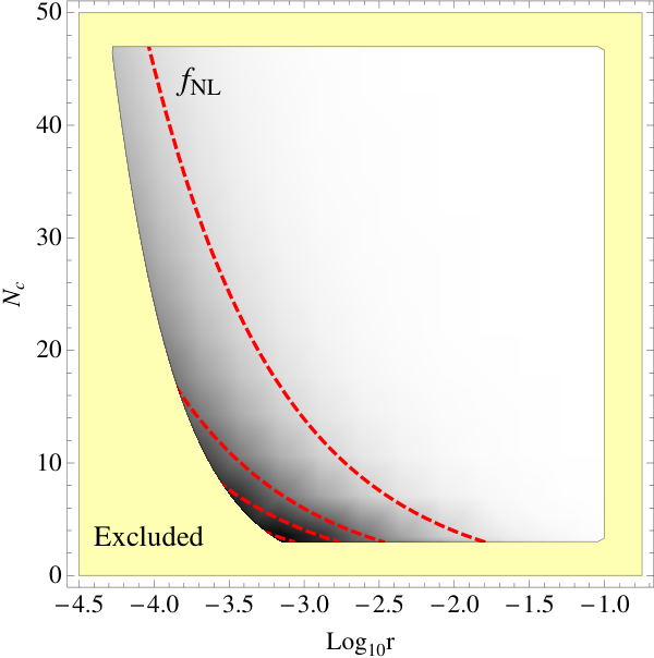
For this model, we have a total of 4 free parameters — $m_{\phi},m_{\sigma},\sigma_{0}$, and $N{}_{c}{}$ – the number of e-folds from the phase boundary “$c$” to the end of inflation. The overall energy scale only affects the power spectrum of curvature perturbation by

$$P_{\zeta}=\frac{16(2N{}_{*}{}+1)m_{\phi}^{2}\sigma_{0}^{2}}{3M_{\mathrm{p}}^{4}}.$$

(58)

Therefore we can fix $P_{\zeta}$ to the observed value and hence reduce the number of parameters to 3. We want $\sigma$ to dominate the curvature perturbations, which requires $\sigma_{0}$ to be large enough ($\sigma_{0}\gg\phi{}_{*}{}$). However as long as this condition is satisfied, the value of $\sigma_{0}$ hardly changes the cosmological predictions of the model. We are left with only two free parameters which are the mass ratio $m_{\sigma}/m_{\phi}$ and $N{}_{c}{}$. For this model the energy density ratio at the phase boundary is given by

$$r=\frac{m_{\sigma}^{2}\sigma_{0}^{2}}{m_{\phi}^{2}\phi{}_{c}{}^{2}},$$

(59)

so we will use $r$ instead of $m_{\sigma}/m_{\phi}$ for the parameter space, together with $N{}_{c}{}$.

After transforming the parameter space, the free parameters reduce from $m_{\phi},m_{\sigma},\sigma_{0},N{}_{c}{}$ to $r$ and $N{}_{c}{}$. The other two degrees of freedom are absorbed in $P_{\zeta}$ which is fixed by observation, and $\sigma_{0}$ which does not change the cosmological predictions. ¹⁰¹⁰ 10 In fact $\sigma_{0}$ changes the inflation energy scale and the ratio of the curvature perturbations by the inflaton and the spectator, but since for $\sigma_{0}\gg\phi{}_{c}{}$, the spectator totally dominates the curvature perturbations and the inflation energy scale is too low to be seen from the primordial gravitational waves, its value does not matter any more. The transformation in the parameter space has the following relations

	$\displaystyle m_{\phi}^{2}$	$\displaystyle=$	$\displaystyle\frac{3M_{\mathrm{p}}^{4}P_{\zeta}}{16(2N{}_{*}{}+1)\sigma_{0}^{2}},$		(60)
	$\displaystyle m_{\sigma}^{2}$	$\displaystyle=$	$\displaystyle\frac{3(2N_{c}+1)M_{\mathrm{p}}^{6}P_{\zeta}}{64(2N_{*}+1)\pi\sigma_{0}^{4}}.$		(61)

The local bispectrum in Eq. (55) now simplifies to (after neglecting the $O(1)$ coefficient)

$$f_{\mathrm{NL}}\sim\frac{1}{(2N_{c}+1)^{2}r}.$$

(62)

The two dimensional parameter space for $r$ and $N{}_{c}{}$ is constrained by the following conditions.

1. 1.

   The Hubble exit of the pivot scale, the phase boundary and the end of inflation are all well separated. So typically we choose $3\leq N{}_{c}{}\leq N{}_{*}{}-3$.

2. 2.

   The $\sigma$ field should be subdominant, so $r\ll 1$.

3. 3.

   The inflaton should provide suppressed curvature perturbations compared to that of the spectator, which means $\sigma_{0}\gg\phi_{*}$.

4. 4.

   The first order slow roll parameter is smaller than unity when $\sigma$ stays on the flat potential, i.e. $\epsilon_{\sigma}{}_{*}{}<1$ and $\epsilon_{\sigma}{}_{c}{}<1$.

5. 5.

   The quantum fluctuations of $\sigma$ should not dominate over its classical slow roll. This means Eq. (47) is valid.

Because of the last constraint, the energy density ratio $r$ can not be too small at the phase boundary. Therefore the maximum possible value $f_{\mathrm{NL}}^{\mathrm{(max)}}\sim 20$ is achieved when $N_{c}=3$ and $r\sim 10^{-3}$.

Under the above conditions, we can calculate the spectral index $n_{s}$, its running $dn_{s}/d\ln k$, the local bispectrum $f_{\mathrm{NL}}$, and the trispectrum $g_{\mathrm{NL}}$, according to Eq. (35), Eq. (39), Eq. (55) and Eq. (56). A specific example of $f_{\mathrm{NL}}$ is shown in Fig 2, for the parameters $N{}_{*}{}=50$, $\sigma_{0}=10M_{\mathrm{p}}$ and $w=1/3$. The regions violating any of the above five conditions are excluded and shown by the yellow shaded region in Fig 2. We can read out from Eq. (60) the mass for $\phi$ here is $m_{\phi}\approx 2.1\times 10^{-7}M_{\mathrm{p}}$, so the curvature perturbations from $\phi$ are indeed negligible. In addition, for these parameters we have $n_{s}=0.98$, $dn_{s}/d\ln k=-3\times 10^{-4}$ and $g_{\mathrm{NL}}\ll 1$, all of which hardly depend on the choice of $N{}_{c}{}$ or $r$, and fall within the observational bound.

From Fig 2, we see that the parameter space is limited. In particular, $r$ is constrained on both the sides because we need $\sigma$ to be subdominant and its quantum fluctuations not to overcome the slow roll motion. Moreover, $\sigma$ hardly contributes to $n_{s}$, $f_{\mathrm{NL}}$ or $g_{\mathrm{NL}}$ because all of its slow roll parameters are tiny. With the inflaton $\phi$ being the only contribution, we get $n_{s}\approx 0.98$, and small running, bispectrum and trispectrum. For these parameters, we can see the local bispectrum strength $f_{\mathrm{NL}}$ indeed has a maximum value around 20. The parameter space for $f_{\mathrm{NL}}>10$ is very limited. In this case the major contribution to $f_{\mathrm{NL}}$ comes from the conversion of the entropy to the curvature perturbations, which becomes non-Gaussian after the spectator ends slow roll and decays into a perfect fluid, even though this non-Gaussian conversion only lasts for one e-fold or so before the entropy perturbations are redshifted away.

Flat directions naturally arise in string theory or supersymmetric theories [5]. These flat directions can also be candidates for $U(\sigma)$. In most cases, such flat directions can be written locally as an effective scalar potential in the form [20, 21]

$$U(\Delta\sigma)=U_{0}\left(1+\gamma_{1}\frac{\Delta\sigma}{M_{\mathrm{p}}}+\frac{\gamma_{3}}{6}\frac{\Delta\sigma^{3}}{M_{\mathrm{p}}^{3}}+O\biggl(\frac{\Delta\sigma^{4}}{M_{\mathrm{p}}^{4}}\biggr)\right),$$

(63)

where

$$\Delta\sigma\equiv\sigma-\sigma_{0}.$$

(64)

Therefore at $\Delta\sigma=0$, i.e. $\sigma=\sigma_{0}$, we will get an inflection/saddle point where $U=U_{0}$ and $U^{\prime\prime}=0$, and $\Delta\sigma$ is the deviation from the inflection point $\sigma_{0}$. For inflection and saddle points we will have $\gamma_{1}>0$ and $\gamma_{1}=0$ respectively, and we always have $\gamma_{3}>0$. In general the higher order terms in the effective potential Eq. (63), e.g. $\Delta\sigma^{4}$, also provide a small contribution to the potential or its derivatives. Here we assume their contribution vanishes for the sake of simplicity.

In this respect the motion of $\sigma$ can be solved as follows. We first obtain the deviation at the phase boundary $\Delta\sigma{}_{c}{}$, from the breakdown of second order slow roll condition $\eta_{\sigma}{}_{c}{}=-1$

$$\Delta\sigma{}_{c}{}=-\frac{8\pi M_{\mathrm{p}}(U_{c}+V_{c})}{\gamma_{3}U_{0}}.$$

(65)

With this we can introduce a very helpful parameter $\gamma_{0}$, which tells us how “flat” the potential is at the inflection point

$$\gamma_{0}\equiv\sqrt{\frac{\gamma_{1}}{M_{\mathrm{p}}}\frac{2M_{\mathrm{p}}^{3}}{\gamma_{3}\Delta\sigma{}_{c}{}^{2}}}=\sqrt{\frac{\gamma_{1}\gamma_{3}}{2}}\,\frac{U_{0}}{4\pi(U{}_{c}{}+V{}_{c}{})}.$$

(66)

Therefore the ratio of $U^{\prime}(\sigma)$ between the inflection point and the phase boundary is $\gamma_{0}/(1+\gamma_{0})$. For the inflection point potential we discuss here, typically $\gamma_{0}\ll 1$.

As long as we specify the inflaton potential and $N{}_{c}{}$, we are able to solve the equation of motion for $\Delta\sigma$. The slow roll approximation in phase I gives the l.h.s of Eq. (8) as

	$\displaystyle\int_{\Delta\sigma{}_{c}{}}^{\Delta\sigma{}_{*}{}}\frac{d\Delta\sigma}{U^{\prime}}$	$\displaystyle=$	$\displaystyle\frac{M_{\mathrm{p}}^{2}}{U_{0}}\sqrt{\frac{2}{\gamma_{1}\gamma_{3}}}\left.\arctan\sqrt{\frac{\gamma_{3}}{2\gamma_{1}}}\,\frac{\Delta\sigma}{M_{\mathrm{p}}}\right|_{c}^{*}$		(67)
		$\displaystyle=$	$\displaystyle\frac{M_{\mathrm{p}}^{2}}{4\pi\gamma_{0}(U{}_{c}{}+V{}_{c}{})}\left(\arctan\frac{1}{\gamma_{0}}+\arctan\frac{x{}_{*}{}}{\gamma_{0}}\right),$

where $x\equiv\Delta\sigma/|\Delta\sigma_{c}|$ is the relative displacement from the inflection point.

Because $\sigma$ always subdominates the energy density, we can neglect its contribution to the Hubble rate and solve the background evolution for $\phi(N)$. By equating Eq. (67) (as the l.h.s of Eq. (8)) with the r.h.s of Eq. (8), we derive the evolution of $\sigma$ by $x_{*}(N_{*})$

$$\arctan\frac{x_{*}}{\gamma_{0}}=-\arctan\frac{1}{\gamma_{0}}+\frac{4\pi\gamma_{0}(U{}_{c}{}+V{}_{c}{})}{M_{\mathrm{p}}^{2}}\int_{\phi{}_{c}{}}^{\phi(N_{*})}\frac{d\phi}{V^{\prime}}.$$

(68)

We can also derive the slow roll parameters that are needed to calculate the cosmological observables

$$\epsilon_{\sigma}=\frac{64\pi^{3}(U_{c}+V_{c})^{4}}{\gamma_{3}^{2}U_{0}^{2}(U+V)^{2}}(\gamma_{0}^{2}+x^{2})^{2},\hskip 21.68121pt\eta_{\sigma}=\frac{U_{c}+V_{c}}{U+V}x,\hskip 21.68121pt\xi_{\sigma}=\frac{(U_{c}+V_{c})^{2}}{2(U+V)^{2}}(\gamma_{0}^{2}+x^{2}),$$

(69)

while all the higher order slow roll parameters vanish. When $\gamma_{3}$ is large and $\gamma_{0}\ll 1$, we have $s_{\sigma}\approx 1$, and the final results are simplified to

	$\displaystyle n_{s}-1$	$\displaystyle=$	$\displaystyle-2\epsilon_{\phi*}+2x_{*},$		(70)
	$\displaystyle\frac{dn_{s}}{d\ln k}$	$\displaystyle\approx$	$\displaystyle-\frac{1}{2}(n_{s}-1)^{2}+2\epsilon_{\phi*}(2\eta_{\phi*}-3\epsilon_{\phi*})+\gamma_{0}^{2}-x_{*}^{2},$		(71)
	$\displaystyle f_{\mathrm{NL}}$	$\displaystyle\approx$	$\displaystyle-\frac{10(5+6w)\epsilon_{\phi c}(2\epsilon_{\phi c}-\eta_{\phi c})}{9(1+w)r}-\frac{5x_{*}}{6r},$		(72)
	$\displaystyle g_{\mathrm{NL}}$	$\displaystyle\approx$	$\displaystyle-\frac{50(5+6w)\epsilon_{\phi c}\xi_{\phi c}}{81(1+w)r^{2}}+\frac{25(3x_{*}^{2}-\gamma_{0}^{2})}{108r^{2}}.$		(73)

References

- (1) C. Bennett, D. Larson, J. Weiland, N. Jarosik, G. Hinshaw, et. al., Nine-Year Wilkinson Microwave Anisotropy Probe (WMAP) Observations: Final Maps and Results, arXiv:1212.5225.
- (2) A. H. Guth, The Inflationary Universe: A Possible Solution to the Horizon and Flatness Problems, Phys.Rev. D23 (1981) 347–356.
- (3) A. D. Linde, A New Inflationary Universe Scenario: A Possible Solution of the Horizon, Flatness, Homogeneity, Isotropy and Primordial Monopole Problems, Phys.Lett. B108 (1982) 389–393.
- (4) A. Albrecht and P. J. Steinhardt, Cosmology for Grand Unified Theories with Radiatively Induced Symmetry Breaking, Phys.Rev.Lett. 48 (1982) 1220–1223.
- (5) A. Mazumdar and J. Rocher, Particle physics models of inflation and curvaton scenarios, Phys.Rept. 497 (2011) 85–215, [arXiv:1001.0993].
- (6) A. R. Liddle, A. Mazumdar, and F. E. Schunck, Assisted inflation, Phys.Rev. D58 (1998) 061301, [astro-ph/9804177].
- (7) A. Ashoorioon, A. Krause, and K. Turzynski, Energy Transfer in Multi Field Inflation and Cosmological Perturbations, JCAP 0902 (2009) 014, [arXiv:0810.4660].
- (8) D. Battefeld, T. Battefeld, C. Byrnes, and D. Langlois, Beauty is Distractive: Particle production during multifield inflation, JCAP 1108 (2011) 025, [arXiv:1106.1891].
- (9) J. Elliston, D. J. Mulryne, D. Seery, and R. Tavakol, Evolution of fNL to the adiabatic limit, JCAP 1111 (2011) 005, [arXiv:1106.2153].
- (10) K. Enqvist and M. S. Sloth, Adiabatic CMB perturbations in pre - big bang string cosmology, Nucl.Phys. B626 (2002) 395–409, [hep-ph/0109214].
- (11) T. Moroi and T. Takahashi, Effects of cosmological moduli fields on cosmic microwave background, Phys.Lett. B522 (2001) 215–221, [hep-ph/0110096].
- (12) D. H. Lyth and D. Wands, Generating the curvature perturbation without an inflaton, Phys.Lett. B524 (2002) 5–14, [hep-ph/0110002].
- (13) D. H. Lyth, C. Ungarelli, and D. Wands, The Primordial density perturbation in the curvaton scenario, Phys.Rev. D67 (2003) 023503, [astro-ph/0208055].
- (14) A. Mazumdar and L. Wang, Creating perturbations from a decaying field during inflation, arXiv:1210.7818.
- (15) R. Allahverdi, R. Brandenberger, F.-Y. Cyr-Racine, and A. Mazumdar, Reheating in Inflationary Cosmology: Theory and Applications, Ann.Rev.Nucl.Part.Sci. 60 (2010) 27–51, [arXiv:1001.2600].
- (16) K. Enqvist, S. Kasuya, and A. Mazumdar, Adiabatic density perturbations and matter generation from the MSSM, Phys.Rev.Lett. 90 (2003) 091302, [hep-ph/0211147].
- (17) K. Enqvist, A. Jokinen, S. Kasuya, and A. Mazumdar, MSSM flat direction as a curvaton, Phys.Rev. D68 (2003) 103507, [hep-ph/0303165].
- (18) R. Allahverdi, K. Enqvist, A. Jokinen, and A. Mazumdar, Identifying the curvaton within MSSM, JCAP 0610 (2006) 007, [hep-ph/0603255].
- (19) A. Mazumdar and S. Nadathur, The curvaton scenario in the MSSM and predictions for non-Gaussianity, Phys.Rev.Lett. 108 (2012) 111302, [arXiv:1107.4078].
- (20) R. Allahverdi, K. Enqvist, J. Garcia-Bellido, A. Jokinen, and A. Mazumdar, MSSM flat direction inflation: Slow roll, stability, fine tunning and reheating, JCAP 0706 (2007) 019, [hep-ph/0610134].
- (21) R. Allahverdi, K. Enqvist, J. Garcia-Bellido, and A. Mazumdar, Gauge invariant MSSM inflaton, Phys.Rev.Lett. 97 (2006) 191304, [hep-ph/0605035].
- (22) S. Davidson and S. Sarkar, Thermalization after inflation, JHEP 0011 (2000) 012, [hep-ph/0009078].
- (23) R. Allahverdi and A. Mazumdar, Reheating in supersymmetric high scale inflation, Phys.Rev. D76 (2007) 103526, [hep-ph/0603244].
- (24) W.-Z. Feng, A. Mazumdar, and P. Nath, Baryogenesis from dark matter in an inflationary universe, arXiv:1302.0012.
- (25) M. Sasaki and E. D. Stewart, A General analytic formula for the spectral index of the density perturbations produced during inflation, Prog.Theor.Phys. 95 (1996) 71–78, [astro-ph/9507001].
- (26) D. Wands, K. A. Malik, D. H. Lyth, and A. R. Liddle, A New approach to the evolution of cosmological perturbations on large scales, Phys.Rev. D62 (2000) 043527, [astro-ph/0003278].
- (27) D. H. Lyth and A. R. Liddle, The primordial density perturbation: Cosmology, inflation and the origin of structure, .
- (28) A. Jokinen and A. Mazumdar, Very large primordial non-gaussianity from multi-field: application to massless preheating, JCAP 0604 (2006) 003, [astro-ph/0512368].
- (29) K. Enqvist, A. Jokinen, A. Mazumdar, T. Multamaki, and A. Vaihkonen, Non-Gaussianity from preheating, Phys.Rev.Lett. 94 (2005) 161301, [astro-ph/0411394].
- (30) A. Mazumdar and L. Wang, Separable and non-separable multi-field inflation and large non-Gaussianity, JCAP 1209 (2012) 005, [arXiv:1203.3558].
- (31) A. D. Linde, Particle physics and inflationary cosmology, Contemp.Concepts Phys. 5 (1990) 1–362, [hep-th/0503203].
- (32) J. M. Bardeen, P. J. Steinhardt, and M. S. Turner, Spontaneous Creation of Almost Scale - Free Density Perturbations in an Inflationary Universe, Phys.Rev. D28 (1983) 679.
- (33) V. F. Mukhanov, H. Feldman, and R. H. Brandenberger, Theory of cosmological perturbations. Part 1. Classical perturbations. Part 2. Quantum theory of perturbations. Part 3. Extensions, Phys.Rept. 215 (1992) 203–333.
- (34) F. Vernizzi and D. Wands, Non-gaussianities in two-field inflation, JCAP 0605 (2006) 019, [astro-ph/0603799].
- (35) J. Smidt, A. Amblard, C. T. Byrnes, A. Cooray, A. Heavens, et. al., CMB Constraints on Primordial non-Gaussianity from the Bispectrum and Trispectrum and a New Consistency Test of Single-Field Inflation, Phys.Rev. D81 (2010) 123007, [arXiv:1004.1409].