Reanalysis of $\mathcal{F}$-statistic gravitational-wave searches with the higher criticism statisticNote: Accepted for publication in The Astrophysical Journal

The higher criticism statistic was introduced by Donoho & Jin [26] to test the hypothesis that $n$ independent and identically distributed (i.i.d.) samples $X_{1},\ldots,X_{n}$ come from the same zero-mean Gaussian distribution $N(0,1)$, against the alternative that a small fraction of them have a nonzero mean $\mu>0$, that is, to test:

For example, $H_{0}$ could correspond to a situation where all samples are just background noise with no signal ($\mu=0$), whereas in $H_{1}$ a fraction $\epsilon$ of samples contain signal ($\mu\neq 0$). Higher criticism is particularly designed for the very challenging situation where the signal is sparse ($\epsilon\ll 1$) and weak ($\mu$ is so small that the largest extreme values under $H_{1}$ are essentially the same as those under $H_{0}$). Although we introduce the statistic in the context of Gaussian noise, it can be generalized easily to other distributions (see Section II.3). The case of correlated, or non-white, noise has been treated by Hall & Jin [28].

Let $Z$ denote a random variable with distribution $N(0,1)$. The higher criticism statistic $HC$ is computed from the $n$ p-values $p_{i}=P[Z>X_{i}]$ generated by the $n$ tests $H_{0,i}:X_{i}\stackrel{{\scriptstyle\mathrm{i.i.d.}}}{{\sim}}N(0,1)$ against $H_{1,i}:X_{i}\stackrel{{\scriptstyle\mathrm{i.i.d.}}}{{\sim}}N(\mu,1)$, $\mu>0$, $i=1,\ldots,n$. It is defined by [26],

where $p_{(1)}\leq p_{(2)}\leq\cdots\leq p_{(n)}$ are the $p_{i}$’s sorted into increasing order. The statistic $HC$ rejects $H_{0}$ when $HC>g(n,\alpha)$, where $g(n,\alpha)$ is a threshold chosen so that $P_{H_{0}}[HC>g(n,\alpha)]=P_{H_{0}}(\textrm{reject $H_{0}$})\leq\alpha$, where $P_{H_{0}}$ denotes the probability when $H_{0}$ is true. [Our notation differs from Donoho & Jin [26] in that we use the symbol $g$ for the threshold instead of $h$ to avoid confusion with the gravitational wave strain $h$.] In other words, the higher criticism test detects a signal when $HC>g(n,\alpha)$. Donoho & Jin [26] showed that, when $H_{0}$ is true, one has $HC\sim\sqrt{2\log\log(n)}$ asymptotically as $n\to\infty$ for all $\alpha>0$, and that if $0<\alpha<1$ and $n$ is large enough, one can use the threshold $g(n,\alpha)\approx\sqrt{2\log\log(n)}$. However for more general $\alpha$ and $n$, this does not work well in practice, as we illustrate in Section II.4, where we discuss how to choose $g(n,\alpha)$ accurately as a function of $n$ and $\alpha$ for finite $n$.

Next, we quantify more precisely how small $\epsilon$ and $\mu$ can be for the test based on $HC$ to be able to distinguish $H_{0}$ from $H_{1}$. Let $r$ and $\beta$ be two positive parameters. Donoho & Jin [26] study the properties of the $HC$ statistic for $\mu$ and $\epsilon$ of the form

These represent very difficult situations since, with $r$ small, $\mu$ of this form is smaller than the mean of the upper extreme statistics, and with $\beta$ large, the proportion of samples with non zero mean is very close to zero. Clearly, a detection is not possible if $r$ is very small and $\beta$ is very large at the same time. Donoho & Jin [26] showed that, as $n\to\infty$, there exists a function $\rho(\beta)$ defined by

such that $H_{0}$ and $H_{1}$ are distinguishable only if $r>\rho(\beta)$. If $r<\rho(\beta)$, there does not exist a test that can distinguish $H_{0}$ from $H_{1}$. Donoho & Jin [26] proved that, under some conditions, the $HC$ statistic is able to distinguish $H_{0}$ from $H_{1}$ throughout the detectable region $r>\rho(\beta)$, and that it has full asymptotic power, that is, $P_{H_{1}}(\textrm{reject $H_{0}$})\to 1$ as $n\to\infty$ (here $P_{H_{1}}$ denotes the conditional probability when $H_{1}$ is true). Another test has also been considered in the literature, namely the Neyman-Pearson likelihood ratio test, but it is less attractive since it requires $r$ and $\beta$ to be known [26], whereas the test based on the higher criticism statistic does not. Interestingly, Donoho & Jin [26] also show that, in addition to the detection boundary, there is a second region $r>\beta$ called the estimable region, where $H_{0}$ and $H_{1}$ can be distinguished and the mean $\mu$ can also be estimated consistently. Figure 1, which can be found in Donoho & Jin [26], illustrates the detectable and estimable regions on the $r$-$\beta$ plane.

In this section, we present briefly some results from Monte-Carlo simulations to illustrate the behavior of $HC$ as a function of signal amplitude $\mu$ and sparsity $\epsilon$ for $n=10^{6}$ sample values drawn randomly from the $H_{1}$ distribution given by equation (2).

Figure 2 displays a histogram of $HC$ values for $10^{3}$ trials with $\epsilon=5\times 10^{-3}$ and $\mu=0,0.1,0.3,1$. Figure 3 displays a similar histogram with $\mu=1$ and $\epsilon=0,5\times 10^{-4},2\times 10^{-3},5\times 10^{-3}$. The top left panel in both figures consists of samples drawn from the null distribution $H_{0}$. As $\mu$ or $\epsilon$ increases, so too does the average value of $HC$.

In Section II.1, we defined $HC$ in the context of Gaussian noise. As shown in Donoho & Jin [26], higher criticism can be generalized to other noise and signal distributions, $\mathcal{N}$ and $\mathcal{S}(\mu)$ say, where $\mu$ describes the amplitude of the signal (e.g. mean of the Gaussian distribution in Section II.1). In this more general setting we test to discriminate between the hypotheses

In this context, the higher criticism statistic is computed as in equation (3), but replacing the $p_{(i)}$’s by the ordered values of $p_{i}=P[Z>X_{i}]$, $i=1,\ldots,n$, where $Z$ is a random variable that has the distribution $\mathcal{N}$; see also Delaigle & Hall [24].

The detection boundary varies with the noise distribution. For example, when $\mathcal{N}$ is the $\chi^{2}$ distribution that we use later, the proportion $\epsilon$ is defined as in equation (5), but the intensity of the signal is defined in terms of the noncentrality parameter $\rho^{2}$ of the $\chi^{2}$ distribution, through

instead of the mean $\mu$ in equation (4). With these definitions of $r$ and $\beta$, the detection boundary is given by equation (6), as in the normal case.

In this section, we discuss the choice of the detection threshold $g(n,\alpha)$ for $HC$. As already noted earlier, the threshold satisfies $P_{H_{0}}[HC>g(n,\alpha)]=P_{H_{0}}(\textrm{reject }H_{0})\leq\alpha$, and under somewhat restrictive conditions, it can be approximated asymptotically by $\sqrt{2\log\log(n)}$. However, in finite samples and under more general conditions, this theoretical value $\sqrt{2\log\log(n)}$ is not a good approximation to $g(n,\alpha)$.

To illustrate this we conduct Monte Carlo simulations to determine the threshold $g(n,\alpha)$ for finite $n$. Note that, when $H_{0}$ is true, the p-values are always independent and identically distributed according to the uniform distribution $U(0,1)$, and thus $g(n,\alpha)$ is independent of the specific noise distribution $\mathcal{N}$. Therefore it suffices to generate p-values from the $U(0,1)$ distribution to compute the threshold. We run $10^{6}$ noise-only simulations with $n=10^{3},10^{4},10^{5},10^{6}$ to determine Monte-Carlo thresholds. For each, we generate $n$ p-values from $U(0,1)$ and compute $HC$.

Figure 4 displays the cumulative distribution function of $HC$ for the simulated noise samples. Threshold values obtained from the simulations by solving an empirical version of $P_{H_{0}}(HC>g(n,\alpha))\approx\alpha$ are listed in Table 1 for $n=10^{3},10^{4},10^{5},10^{6}$ and $\alpha=0.5,0.1,0.05,0.01$. For comparison, the theoretical value $\sqrt{2\log\log(n)}$ is also quoted. From this and Figure 4, we can see that this theoretical value generally does not work well in practice. In each case, a large fraction ($\gtrsim$ 50%) of noise-only trials fall above this threshold. In the remainder of this paper, we commonly use the threshold $g(n,0.01)$ as determined from Monte-Carlo simulations with $\alpha=0.01$ (1% false alarm rate).

The gravitational wave signal from a neutron star in a binary has its frequency modulated into sidebands with spacing $1/P$, where $P$ is the orbital period [34]. Therefore, an $\mathcal{F}$-statistic search sees a large number of relatively weak signals across many frequency bands. For a neutron star with intrinsic gravitational wave frequency $f_{0}$, $2\mathcal{F}$ obeys a $\chi^{2}_{4}[\rho^{2}(f)]$ distribution, where the frequency dependent noncentrality parameter can be written [34]

with $Z_{0}=2\pi f_{0}a$, where $\lfloor{Z_{0}}\rfloor$ represents the largest integer less than $Z_{0}$, $J_{n}$ is the $n$-th order Bessel function of the first kind, $a$ is the light crossing time of the orbital radius projected onto the line of sight, $f_{0,n}=f_{0}-n/P$ is the frequency of the $n$th sideband around a source with frequency $f_{0}$, $\rho_{0}^{2}$ is the source signal-to-noise ratio squared [see equation (10)], and $\tilde{W}(f)$ is the Fourier transform of the window function $W(t)$, which equals 1 or 0 when the detector is on or off respectively. Assuming no gaps in the data, one finds

With the window function defined as in Messenger & Woan [34], an extra factor of $1/T_{obs}^{2}$ is included in equation (16) so that $\mathcal{C}$ is dimensionless.

The $\mathcal{C}$-statistic sums incoherently the $\mathcal{F}$-statistic power in the orbital sidebands [34] as follows:

For noise only, $2\mathcal{F}$ is distributed according to a $\chi^{2}_{4}$ distribution. Hence, $\mathcal{C}$, which is the sum of $M\;$ $2\mathcal{F}$ values, obeys a $\chi^{2}_{4M}$ distribution, where $M=2\lfloor{Z_{0}}\rfloor+1$ is the total number of sidebands [34]. In the presence of a signal, $2\mathcal{F}(f)$ is distributed according to a noncentral $\chi^{2}_{4}[\rho^{2}(f)]$ distribution with a frequency dependent noncentrality parameter $\rho^{2}(f)$ and $\mathcal{C}$ follows a noncentral $\chi^{2}_{4M}(\lambda)$ distribution with noncentrality parameter [34]

How does a $\mathcal{C}$-statistic search, which assumes that $P$ (and hence the sideband locations) are known, perform in comparison with a second-pass higher criticism search over $\mathcal{F}$-statistic or $\mathcal{C}$-statistic values? We run Monte-Carlo simulations to answer this question.

We simulate a targeted search for Sco X-1, similar to the one described in Sammut et al. (2013, in preparation) . The search parameters are $P=68023.84$ s, $a=1.44$ s, $T_{obs}=10$ days, and source frequency $f_{0}=400$ Hz (assumed). We search over the range of frequencies $100\leq f\leq 1000$ Hz with frequency bin spacing $\delta f=1/(2T_{obs})=5.8\times 10^{-7}$ Hz, corresponding to $n=1.5\times 10^{9}$ frequency bins in total. The signal is modulated into $M$ sidebands separated by $1/P$. $M$ depends on the signal frequency, with $1811\leq M\leq 18097$ for 100 Hz $\leq f_{0}\leq$ 1000 Hz. The width in frequency space of the entire sideband structure (the comb) is 0.03 Hz $\leq M/P\leq$ 0.27 Hz.

Let us apply higher criticism to the problem. We take advantage of the relatively narrow sideband structure and divide the frequency domain $[f_{min},f_{max}]$ into $N_{w}$ windows of equal width $w$, each containing $n_{w}$ frequency bins, viz. $[f_{min},f_{min}+w]$, $[f_{min}+w/2,f_{min}+3w/2]$, $[f_{min}+w,f_{min}+2w]$, …, $[f_{max}-3w/2,f_{max}-w/2]$, $[f_{max}-w,f_{max}]$. The width $w$ is chosen to be twice the maximum width of the sidebands, $w=2M/P$, and windows overlap by 50% to ensure that the entire signal is contained entirely within a single window. A more sophisticated method would vary the width with frequency as the sideband width increases from 0.03 Hz for $f_{0}=100$ Hz to 0.27 Hz for $f_{0}=1000$ Hz, however, for simplicity, we construct our search windows based on the maximum sideband width at $f_{max}=1000$ Hz, obtaining $w=0.53$ Hz, $n_{w}=9.2\times 10^{5}$, and $N_{w}=3.4\times 10^{3}$.

The data are synthesized as follows. First, the noncentrality parameter is computed for each frequency bin. The signal is modulated into sidebands and the frequency dependent noncentrality can be written (Sammut et al. 2013, in preparation) ,

We simplify this equation assuming $\left|\tilde{W}(f)\right|^{2}\approx\delta(f)$ (true in the limit $T_{obs}\to\infty$) and assume the $J_{n}^{2}(Z_{0})$ all have similar amplitude, which we absorb into the constant $\rho_{0}^{2}$. Additionally, we adjust the frequency of each sideband $f_{0,n}$ to be equal to the corresponding closest frequency bin, $\textrm{nr}(f_{0,n})$, using $\textrm{nr}(f)$ to represent the frequency bin closest to frequency $f$, neglecting the potential loss of amplitude caused by the mismatch between $f_{0,n}$ and $\textrm{nr}(f_{0,n})$. We denote the frequency on the $i$-th frequency bin $f^{\prime}_{i}$, using the ‘prime’ notation to differentiate between frequency bins and the exact frequency of the signal $f_{0}$ or the sidebands $f_{0,n}$. The simplified noncentrality parameter used to generate the $\mathcal{F}$-statistic for each frequency bin $f^{\prime}_{i}$ is

where $K(x,y)=\delta_{x,y}$ is the standard Kronecker delta rebranded so that we can see the subscripts clearly. Equation (20) corresponds to $\rho^{2}(f^{\prime}_{i})$ equal to $\rho_{0}^{2}$ for the frequency bin closest to each of the true sideband locations and zero elsewhere. We generate synthetic $2\mathcal{F}$ values drawn from the $\chi^{2}_{4}[\rho^{2}(f^{\prime}_{i})]$ distribution, for each frequency bin $f^{\prime}_{i}$.

To compute $\mathcal{C}$-statistic values, we construct a comb centered at each frequency bin $f^{\prime}_{i}$ assuming $f_{0}=f^{\prime}_{i}$,

with $Z^{\prime}_{i}=2\pi f^{\prime}_{i}a$ and $f^{\prime}_{i,n}=f^{\prime}_{i}+n/P$. The $\mathcal{C}$-statistic is computed by convolving the $2\mathcal{F}(f)$ with $q(f)$ [34]

We compute the higher criticism statistic as described in Section II.3 for the $2\mathcal{F}$ and the $\mathcal{C}$ values contained in a given search window and call the results $HC_{2\mathcal{F}}$ and $HC_{\mathcal{C}}$ respectively. The noise distribution for $2\mathcal{F}$ is $\chi^{2}_{4}(0)$. It is more complicated for $\mathcal{C}$, as the number of sidebands $M^{\prime}_{i}=2\lfloor{Z^{\prime}_{i}}\rfloor+1$ depends on the frequency $f^{\prime}_{i}$. Hence, the p-values for each $\mathcal{C}(f^{\prime}_{i})$ are calculated with respect to the $\chi^{2}_{4M^{\prime}_{i}}$ noise distribution (four degrees of freedom for each sideband summed).

To compare the performance of the three detection statistics $\mathcal{C}$, $HC_{2\mathcal{F}}$ and $HC_{\mathcal{C}}$, we compute thresholds with a false alarm rate $\alpha=0.01$. We have $n$ $2\mathcal{F}$ and $\mathcal{C}$ values, one for each frequency bin, and $N_{w}$ $HC_{2\mathcal{F}}$ and $HC_{\mathcal{C}}$ values, one for each search window. Thresholds are found by insisting that noise-only data fall below the threshold in every bin or window with probability at least $1-\alpha$ [e.g., Wette [39]],

where $\mathcal{C}_{th}(\alpha)$ is the $\mathcal{C}$-statistic threshold. The $HC$ threshold $g(n_{\mathrm{w}},\alpha)$ is determined from Monte-Carlo simulations, as described in Section II.4. We integrate the $\mathcal{C}$-statistic probability distribution to find $\mathcal{C}_{th}(\alpha)$ and use the result to compute the threshold noncentrality parameter $\lambda_{th}(\alpha,\delta)$ for false dismissal rate $\delta=0.1$ from

where $F(x;k,\lambda)$ is the probability density function of the $\chi^{2}_{k}(\lambda)$ distribution and $4M^{\prime}_{i,max}$ is the maximum number of sidebands for all $f^{\prime}_{i}$ in the window.

To simulate the gravitational wave search, we choose $\rho^{2}_{0}$ and draw $2\mathcal{F}$ values from the $\chi^{2}_{4}[\rho^{2}(f^{\prime}_{i})]$ distribution for each frequency bin $f^{\prime}_{i}$. The search windows are constructed to ensure the entire sideband structure lies completely within a single window. Sidebands are also present in adjacent windows, however we focus only on a single window, assuming (conservatively) that all other windows contain only noise. Equation (24) makes the same assumption when computing the detection thresholds against which $HC_{2\mathcal{F}}$ and $HC_{\mathcal{C}}$ are compared. We conduct a 100 Monte-Carlo simulations for each $\rho^{2}_{0}$ and find the fraction where the computed statistic lies above its threshold value, which we call the detection rate.

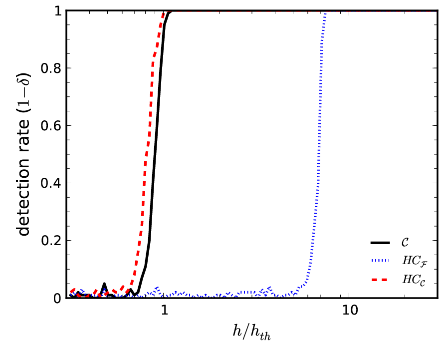
Figure 5 displays detection rates for $\mathcal{C}$, $HC_{2\mathcal{F}}$, and $HC_{\mathcal{C}}$ as functions of increasing wave strain $h/h_{th}$, where $h_{th}$ is defined as the wave strain corresponding to $\lambda_{th}$. For $\delta=0.1$ (detection rate of 90%), $HC_{\mathcal{C}}$ detects wave strains 6% smaller than $\mathcal{C}$ alone and $HC_{2\mathcal{F}}$ detects wave strains $\sim 7$ times greater than $\mathcal{C}$. Additionally, higher criticism on $2\mathcal{F}$ compared to $2\mathcal{F}$ provides a advantage comparable to $HC_{\mathcal{C}}$ over $\mathcal{C}$ (not displayed in Figure 5). The results in Figure 5 assume perfect knowledge of the binary orbital period $P$. In summary, therefore, second-pass higher criticism on $\mathcal{C}$ slightly boosts the sensitivity of the $\mathcal{C}$-statistic, while second-pass higher criticism on $2\mathcal{F}$ is not competitive. Both higher criticism statistics, in particular $HC_{2\mathcal{F}}$, are more robust than $\mathcal{C}$, as demonstrated in the next section.

One significant advantage of higher criticism is its robustness when applied to signals that differ from the assumed form, e.g. due to phase wandering. In this section, we explore the performance of the statistics $\mathcal{C}$, $HC_{\mathcal{C}}$, and $HC_{2\mathcal{F}}$ when the form of the signal remains unaltered but the true signal parameters differ from those assumed in the search. For a comb search targeting a binary source, the orbital period $P$ determines the sideband spacing of the $\mathcal{F}$-statistic in the frequency domain. An error $\Delta P$ between the assumed and true value of $P$ produces a comb that does not coincide with the actual sidebands. The $\mathcal{C}$-statistic sums noise at each sideband whose frequency does not match a true sideband location, lowering the sensitivity. In contrast, $HC_{2\mathcal{F}}$ only assumes that all sidebands are located within a particular frequency window. It does not rely on knowledge of the precise location of each sideband and consequently is unaffected by an error in $P$. Both $HC_{\mathcal{C}}$ and the $\mathcal{C}$-statistic lose sensitivity as $\Delta P$ increases, however one would expect the relative advantage of $HC_{\mathcal{C}}$ compared to $\mathcal{C}$ is expected to remain.

Observations of the orbital period of Sco X-1 have reported conflicting values for $P$. Gottlieb et al. [27] measured $P=68023.8\pm 0.09$ s from archival optical observations. Recently, Vanderlinde et al. [36] measured $P=68163.6\pm 8.6$ s with the Rossi X-ray Timing Explorer, but did not observe any signification periodicity at or near the previously reported value of 68023.8 s. Other LMXBs have larger uncertainty in their orbital parameters [e.g., see Tables 2–4 in Watts et al. [38]]. In light of the potential uncertainty in $P$, the robustness of higher criticism is valuable.

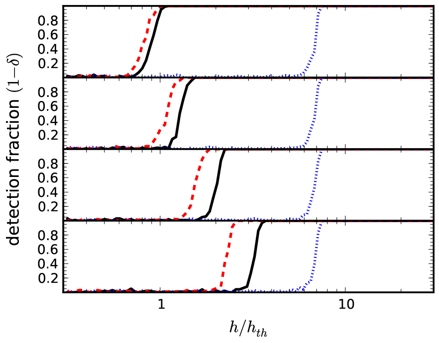
We repeat the simulations described in Section IV.2 with the addition of an error $\Delta P$ between the assumed value of $P$ used to construct the comb $q(f)$, and the true value used to generate the noncentrality parameters $\rho^{2}(f)$ for the $\mathcal{F}$-statistic at every sideband. Figure 6 displays detection rates with $\mathcal{C}$, $HC_{2\mathcal{F}}$, and $HC_{\mathcal{C}}$ as $\Delta P$ increases. As expected, $HC_{2\mathcal{F}}$ is unaffected by $\Delta P$ because higher criticism does not use any information about the sideband locations. $\mathcal{C}$ and $HC_{\mathcal{C}}$ both lose sensitivity as $\Delta P$ increases, but the relative advantage of $HC_{\mathcal{C}}$ over $\mathcal{C}$ increases from 6% when $\Delta P=0$ to 15% for $\Delta P=1$ s, 21% for $\Delta P=3$ s, and 29% for $\Delta P=9$ s. The difference between $\mathcal{C}$ and $HC_{2\mathcal{F}}$ decreases from a factor of 7 when $\Delta P=0$ to 5 for $\Delta P=1$ s, 3 for $\Delta P=3$ s, and 2 for $\Delta P=9$ s. When $\Delta P=0$, the $\mathcal{C}$-statistic peaks at the signal frequency $f_{0}$. For $\Delta P>0$, the error between the assumed and actual location of the sidebands accumulates to the point where the outermost sidebands no longer coincide with the assumed comb. This reduces the total number of signal sidebands summed by the $\mathcal{C}$-statistic, reducing its maximum amplitude (at $f_{0}$). Additionally, the $\mathcal{C}$-statistic peak broadens compared with $\Delta P=0$; this maximum amplitude requires less signal bins summed and can now be reached at a number of the central sidebands. This situation moves closer to multiple, equal-strength signals, the problem for which higher criticism is designed, explaining the increasing advantage of $HC_{\mathcal{C}}$ over $\mathcal{C}$. In contrast, the $\mathcal{C}$-statistic requires a single source above threshold for detection. Interestingly, the sensitivity decrease of $\mathcal{C}$ and $HC_{\mathcal{C}}$ stalls for 9 s $\lesssim\Delta P\lesssim$ 1000 s, when the accumulated error at the outermost sidebands is at least the sideband spacing. At this point, sidebands begin to overlap with other parts of the comb, shifted by integer multiples of the sideband spacing. As $\Delta P$ increases beyond 9 s, the number of sidebands correctly located by the template continues to decrease but is compensated for by a corresponding increase in the number of integer overlap sidebands.

References

- [1] Abadie, J., Abbott, B. P., Abbott, R., et al. 2010a, ApJ, 722, 1504
- [2] —. 2010b, Classical and Quantum Gravity, 27, 173001
- [3] —. 2011, ApJ, 737, 93
- [4] Abbott, B., Abbott, R., Adhikari, R., et al. 2004, Phys. Rev. D, 69, 082004
- [5] —. 2005, Phys. Rev. D, 72, 102004
- [6] —. 2007a, Phys. Rev. D, 76, 082001
- [7] —. 2007b, Phys. Rev. D, 76, 042001
- [8] —. 2008a, Phys. Rev. D, 77, 022001
- [9] —. 2008b, ApJ, 683, L45
- [10] —. 2009a, Phys. Rev. D, 79, 022001
- [11] Abbott, B. P., Abbott, R., Adhikari, R., et al. 2009b, Physical Review Letters, 102, 111102
- [12] —. 2009c, Phys. Rev. D, 80, 042003
- [13] —. 2009d, Reports on Progress in Physics, 72, 076901
- [14] . 2012, Journal of Instrumentation, 7, 3012
- [15] Arnett, W. D., Schramm, D. N., & Truran, J. W. 1989, ApJ, 339, L25
- [16] Bildsten, L. 1998, ApJ, 501, L89+
- [17] Brady, P. R., & Creighton, T. 2000, Phys. Rev. D, 61, 082001
- [18] Cayón, L., Jin, J., & Treaster, A. 2005, MNRAS, 362, 826
- [19] Chakrabarty, D., Morgan, E. H., Muno, M. P., et al. 2003, Nature, 424, 42
- [20] Cook, G. B., Shapiro, S. L., & Teukolsky, S. A. 1994, ApJ, 424, 823
- [21] Cutler, C. 2011, arXiv:1104.2938
- [22] Cutler, C., Gholami, I., & Krishnan, B. 2005, Phys. Rev. D, 72, 042004
- [23] Cutler, C., & Schutz, B. F. 2005, Phys. Rev. D, 72, 063006
- [24] Delaigle, A., & Hall, P. 2009, in Perspectives in mathematical sciences I: Probability and Statistics, ed. B. R. N. Sastry, M. Delampady & T. Rao (World Scientific Publishing), 109–138
- [25] Delaigle, A., Hall, P., & Jin, J. 2011, Journal of the Royal Statistical Society: Series B (Statistical Methodology), 73, 283
- [26] Donoho, D., & Jin, J. 2004, Annals of Statistics, 32, 962
- [27] Gottlieb, E. W., Wright, E. L., & Liller, W. 1975, ApJ, 195, L33
- [28] Hall, P., & Jin, J. 2010, Annals of Statistics, 38, 1686
- [29] Jaranowski, P., Królak, A., & Schutz, B. F. 1998, Phys. Rev. D, 58, 063001
- [30] Krishnan, B., Sintes, A. M., Papa, M. A., et al. 2004, Phys. Rev. D, 70, 082001
- [31] Manchester, R. N., Hobbs, G. B., Teoh, A., & Hobbs, M. 2005, AJ, 129, 1993
- [32] Mastrano, A., & Melatos, A. 2012, MNRAS, 421, 760
- [33] Melatos, A., & Payne, D. J. B. 2005, ApJ, 623, 1044
- [34] Messenger, C., & Woan, G. 2007, Classical and Quantum Gravity, 24, 469
- [35] Ushomirsky, G., Cutler, C., & Bildsten, L. 2000, MNRAS, 319, 902
- [36] Vanderlinde, K. W., Levine, A. M., & Rappaport, S. A. 2003, PASP, 115, 739
- [37] Vigelius, M., & Melatos, A. 2009, MNRAS, 395, 1972
- [38] Watts, A. L., Krishnan, B., Bildsten, L., & Schutz, B. F. 2008, MNRAS, 389, 839
- [39] Wette, K. 2012, Phys. Rev. D, 85, 042003
Appendix A All-sky search
One might ask whether higher criticism can be applied profitably to all-sky searches. After all, from an estimated Galactic population of neutron stars [15], only pulsars have been discovered as radio sources, of which % have frequencies in the range where current interferometers are most sensitive, Hz [31]11 1 http://www.atnf.csiro.au/research/pulsar/psrcat. Theories of neutron star quadrupoles suggest that only a handful of the observed pulsars have any chance of being detectable with current sensitivity limits [32], but many of the radio-quiet objects are much closer to the Earth than their radio-loud brethren. All-sky searches cover a range of frequencies at many sky locations, hoping to detect one of these unknown sources. A number of all-sky searches have been carried out [5, 6, 8, 10, 11, 12], but no detection has been announced. The searches typically use the -statistic, or related statistics. Hence they are candidates for reanalysis with higher criticism.
In contrast to the other applications in this paper, the sources targeted by an all-sky search have a power law (non-uniform) wave strain distribution. We follow Cutler & Schutz [23] and assume neutron stars are spread uniformly throughout the Galaxy. Then the distance distribution separates into two parts: a local uniform three-dimensional distribution up to the thickness of the Galactic disk, and a uniform two-dimensional distribution beyond. Taking the disk to be 600 pc thick and 10 kpc in diameter, the 3D and 2D distributions correspond to pc and 300 pc 5 kpc respectively, where is the distance from Earth. We further assume that all sources have the same intrinsic amplitude, so that at Earth depends on distance alone. Changing variables from distance to noncentrality parameter , [see equation (10); also Cutler & Schutz [23] for details] we arrive at the distribution,