Untitled Document

Foundations of
Descriptive and Inferential
Statistics

Lecture notes for a quantitative–methodological module at the Bachelor degree (B.Sc.) level

Henk van Elst

August 30, 2019

parcIT GmbH

Erftstraße 15

50672 Köln

Germany

E–Mail: Henk.van.Elst@parcIT.de

E–Print: arXiv:1302.2525v4 [stat.AP]

Abstract

These lecture notes were written with the aim to provide an accessible though technically solid introduction to the logic of systematical analyses of statistical data to both undergraduate and postgraduate students, in particular in the Social Sciences, Economics, and the Financial Services. They may also serve as a general reference for the application of quantitative–empirical research methods. In an attempt to encourage the adoption of an interdisciplinary perspective on quantitative problems arising in practice, the notes cover the four broad topics (i) descriptive statistical processing of raw data, (ii) elementary probability theory, (iii) the operationalisation of one-dimensional latent statistical variables according to Likert’s widely used scaling approach, and (iv) null hypothesis significance testing within the frequentist approach to probability theory concerning (a) distributional differences of variables between subgroups of a target population, and (b) statistical associations between two variables. The relevance of effect sizes for making inferences is emphasised. These lecture notes are fully hyperlinked, thus providing a direct route to original scientific papers as well as to interesting biographical information. They also list many commands for running statistical functions and data analysis routines in the software packages R, SPSS, EXCEL and OpenOffice. The immediate involvement in actual data analysis practices is strongly recommended.

Cite as: arXiv:1302.2525v4 [stat.AP]

These lecture notes were typeset in LaTeX 2ε.

Introductory remarks

Statistical methods of data analysis form the cornerstone of quantitative–empirical research in the Social Sciences, Humanities, and Economics. Historically, the bulk of knowledge available in Statistics emerged in the context of the analysis of (nowadays large) data sets from observational and experimental measurements in the Natural Sciences. The purpose of the present lecture notes is to provide its readers with a solid and thorough, though accessible introduction to the basic concepts of Descriptive and Inferential Statistics. When discussing methods relating to the latter subject, we will here take the perspective of the frequentist approach to Probability Theory. (See Ref. [20] for a methodologically different approach.)

The concepts to be introduced and the topics to be covered have been selected in order to make available a fairly self-contained basic statistical tool kit for thorough analysis at the univariate and bivariate levels of complexity of data, gained by means of opinion polls, surveys or observation.

In the Social Sciences, Humanities, and Economics there are two broad families of empirical research tools available for studying behavioural features of and mutual interactions between human individuals on the one-hand side, and the social systems and organisations that these form on the other. Qualitative–empirical methods focus their view on the individual with the aim to account for her/his/its particular characteristic features, thus probing the “small scale-structure” of a social system, while quantitative–empirical methods strive to recognise patterns and regularities that pertain to a large number of individuals and so hope to gain insight on the “large-scale structure” of a social system.

Both approaches are strongly committed to pursuing the principles of the scientific method. These entail the systematic observation and measurement of phenomena of interest on the basis of well-defined statistical variables, the structured analysis of data so generated, the attempt to provide compelling theoretical explanations for effects for which there exists conclusive evidence in the data, the derivation from the data of predictions which can be tested empirically, and the publication of all relevant data and the analytical and interpretational tools developed and used, so that the pivotal replicability of a researcher’s findings and associated conclusions is ensured. By complying with these principles, the body of scientific knowledge available in any field of research and its practical applications undergoes a continuing process of updating and expansion.

Having thoroughly worked through these lecture notes, a reader should have obtained a good understanding of the use and efficiency of descriptive and frequentist inferential statistical methods for handling quantitative issues, as they often arise in a manager’s everyday business life. Likewise, a reader should feel well-prepared for a smooth entry into any Master degree programme in the Social Sciences or Economics which puts emphasis on quantitative–empirical methods.

Following a standard pedagogical concept, these lecture notes are split into three main parts: Part I, comprising Chapters 1 to 5, covers the basic considerations of Descriptive Statistics; Part II, which consists of Chapters 6 to 8, introduces the foundations of Probability Theory. Finally, the material of Part III, provided in Chapters 9 to 13, first reviews a widespread method for operationalising latent statistical variables, and then introduces a number of standard uni- and bivariate analytical tools of Inferential Statistics within the frequentist framework that prove valuable in applications. As such, the contents of Part III are the most important ones for quantitative–empirical research work. Useful mathematical tools and further material have been gathered in appendices.

Recommended introductory textbooks, which may be used for study in parallel to these lecture notes, are Levin et al (2010) [62], Hatzinger and Nagel (2013) [38], Weinberg and Abramowitz (2008) [116], Wewel (2014) [117], Toutenburg (2005) [109], or Duller (2007) [17].

There are not included in these lecture notes any explicit exercises on the topics to be discussed. These are reserved for lectures given throughout term time.

The present lecture notes are designed to be dynamical in character. On the one-hand side, this means that they will be updated on a regular basis. On the other, that the *.pdf version of the notes contains interactive features such as fully hyperlinked references to original publications at the websites doi.org and jstor.org, as well as many active links to biographical information on scientists that have been influential in the historical development of Probability Theory and Statistics, hosted by the websites The MacTutor History of Mathematics archive (www-history.mcs.st-and.ac.uk) and en.wikipedia.org.

Throughout these lecture notes references have been provided to respective descriptive and inferential statistical functions and routines that are available in the excellent and widespread statistical software package R, on a standard graphic display calculator (GDC), and in the statistical software packages EXCEL, OpenOffice and SPSS (Statistical Program for the Social Sciences). R and its exhaustive documentation are distributed by the R Core Team (2019) [86] via the website cran.r-project.org. R, too, has been employed for generating all the figures contained in these lecture notes. Useful and easily accessible textbooks on the application of R for statistical data analysis are, e.g., Dalgaard (2008) [16], or Hatzinger et al (2014) [39]. Further helpful information and assistance is available from the website www.r-tutor.com. For active statistical data analysis with R, we strongly recommend the use of the convenient custom-made work environment R Studio, provided free of charge at www.rstudio.com. Another user friendly statistical software package is GNU PSPP. This is available as shareware from www.gnu.org/software/pspp/.

A few examples from the inbuilt R data sets package have been related to in these lecture notes in the context of the visualisation of distributional features of statistical data. Further information on these data sets can be obtained by typing library(help = "datasets") at the R prompt.

Lastly, we hope the reader will discover something useful or/and enjoyable for her/him-self when working through these lecture notes. Constructive criticism is always welcome.

Acknowledgments: I am grateful to Kai Holschuh, Eva Kunz and Diane Wilcox for valuable comments on an earlier draft of these lecture notes, to Isabel Passin for being a critical sparing partner in evaluating pedagogical considerations concerning cocreated accompanying lectures, and to Michael Rüger for compiling an initial list of online survey tools for the Social Sciences.

Chapter 1 Statistical variables

A central task of an empirical scientific discipline is the observation or measurement of a finite set of characteristic variable features of a given system of objects chosen for study. The hope is to be able to recognise in a sea of data, typically guided by randomness, meaningful patterns and regularities that provide evidence for possible associations, or, stronger still, causal relationships between these variable features. Based on a combination of inductive and deductive methods of data analysis, one aims at gaining insights of a qualitative and/or quantitative nature into the intricate and often complex interdependencies of such variable features for the purpose of (i) obtaining explanations for phenomena that have been observed, and (ii) making predictions which, subsequently, can be tested. The acceptance of the validity of a particular empirical scientific framework generally increases with the number of successful replications of its predictions.¹¹ 1 A particularly sceptical view on the ability of making reliable predictions in certain empirical scientific disciplines is voiced in Taleb (2007) [106, pp 135–211]. It is the interplay of observation, experimentation and theoretical modelling, systematically coupled to one another by a number of feedback loops, which gives rise to progress in learning and understanding in all empirical scientific activities. This procedure, which focuses on replicable facts, is referred to as the scientific method.

More specifically, the general intention of empirical scientific activities is to modify or strengthen the theoretical foundations of an empirical scientific discipline by means of observational and/or experimental testing of sets of hypotheses; see Ch. 11. This is generally achieved by employing the quantitative–empirical techniques that have been developed in Statistics, in particular in the course of the $20^{\mathrm{th}}$ Century. At the heart of these techniques is the concept of a statistical variable $X$ as an entity which represents a single common aspect of the system of objects selected for analysis — the target population $\boldsymbol{\Omega}$ of a statistical investigation. In the ideal case, a variable entertains a one-to-one correspondence with an observable, and thus is directly amenable to measurement. In the Social Sciences, Humanities, and Economics, however, one needs to carefully distinguish between manifest variables corresponding to observables on the one-hand side, and latent variables representing in general unobservable “social constructs” on the other. It is this latter kind of variables which is commonplace in the fields mentioned. Hence, it becomes an unavoidable task to thoroughly address the issue of a reliable, valid and objective operationalisation of any given latent variable one has identified as providing essential information on the objects under investigation. A standard approach to dealing with the important matter of rendering latent variables measurable is reviewed in Ch. 9.

In Statistics, it has proven useful to classify variables on the basis of their intrinsic information content into one of three hierachically ordered categories, referred to as the scale levels of measurement; cf. Stevens (1946) [99]. We provide the definition of these scale levels next.

1.1 Scale levels of measurement

Def.: Let $X$ be a one-dimensional statistical variable with $k\in\mathbb{N}$ (countably many) resp. $k\in\mathbb{R}$ (uncountably many) possible values, attributes, or categories $a_{j}$ ( $j=1,\ldots,k$ ). Statistical variables are classified as belonging into one of three hierachically ordered scale levels of measurement. This is done on the basis of three criteria for distinguishing information contained in the values of actual data for these variables. One thus defines:

•
Metrically scaled variables $X$ (quantitative/numerical)
Possible values can be distinguished by
- (i)
  
  their names, $a_{i}\neq a_{j}$ ,
- (ii)
  
  they allow for a natural rank order, $a_{i}<a_{j}$ , and
- (iii)
  
  distances between them, $a_{i}-a_{j}$ , are uniquely determined.
- –
  
  Ratio scale: $X$ has an absolute zero point and otherwise only non-negative values; analysis of both differences $a_{i}-a_{j}$ and ratios $a_{i}/a_{j}$ is meaningful.
  
  Examples: body height, monthly net income, ….
- –
  
  Interval scale: $X$ has no absolute zero point; only differences $a_{i}-a_{j}$ are meaningful.
  
  Examples: year of birth, temperature in centigrades, Likert scales (cf. Ch. 9), ….
Note that the values obtained for a metrically scaled variable (e.g. in a survey) always constitute definite numerical multiples of a specific unit of measurement.
•
Ordinally scaled variables $X$ (qualitative/categorical)
Possible values, attributes, or categories can be distinguished by
- (i)
  
  their names, $a_{i}\neq a_{j}$ , and
- (ii)
  
  they allow for a natural rank order, $a_{i}<a_{j}$ .
Examples: Likert item rating scales (cf. Ch. 9), grading of commodities, ….
•
Nominally scaled variables $X$ (qualitative/categorical)
Possible values, attributes, or categories can be distinguished only by
- (i)
  
  their names, $a_{i}\neq a_{j}$ .
Examples: first name, location of birth, ….

Remark: As we will see later in Ch. 12 and 13, the applicability of specific methods of statistical data analysis crucially depends on the scale level of measurement of the variables involved in the respective procedures. Metrically scaled data offers the largest variety of powerful methods for this purpose!

1.2 Raw data sets and data matrices

To set the stage for subsequent considerations, we here introduce some formal representations of entities which assume central roles in statistical data analyses.

Let $\boldsymbol{\Omega}$ denote the target population of study objects of interest (e.g., human individuals forming a particular social system) relating to some statistical investigation. This set $\boldsymbol{\Omega}$ shall comprise a total of $N\in\mathbb{N}$ statistical units, i.e., its size be $|\boldsymbol{\Omega}|=N$ .

Suppose one intends to determine the frequency distributional properties in $\boldsymbol{\Omega}$ of a portfolio of $m\in\mathbb{N}$ statistical variables $X$ , $Y$ , …, and $Z$ , with spectra of values $a_{1},a_{2},\ldots,a_{k}$ , $b_{1},b_{2},\ldots,b_{l}$ , …, and $c_{1},c_{2},\ldots,c_{p}$ , respectively ( $k,l,p\in\mathbb{N}$ ). A survey typically obtains from $\boldsymbol{\Omega}$ a statistical sample $\boldsymbol{S_{\Omega}}$ of size $|\boldsymbol{S_{\Omega}}|=n$ ( $n\in\mathbb{N}$ , $n<N$ ), unless one is given the rare opportunity to conduct a proper census on $\boldsymbol{\Omega}$ (in which case $n=N$ ). The data thus generated consists of observed values $\{x_{i}\}_{i=1,\ldots,n}$ , $\{y_{i}\}_{i=1,\ldots,n}$ , …, and $\{z_{i}\}_{i=1,\ldots,n}$ . It constitutes the raw data set $\{(x_{i},y_{i},\ldots,z_{i})\}_{i=1,\ldots,n}$ of a statistical investigation and may be conveniently assembled in the form of an $\boldsymbol{(n\times m)}$ data matrix $\boldsymbol{X}$ given by

sampling	variable	variable	…	variable
unit	$X$	$Y$		$Z$
$1$	$x_{1}=a_{5}$	$y_{1}=b_{9}$	…	$z_{1}=c_{3}$
$2$	$x_{2}=a_{2}$	$y_{2}=b_{12}$	…	$z_{2}=c_{8}$
⋮	⋮	⋮	⋮	⋮
$n$	$x_{n}=a_{8}$	$y_{n}=b_{9}$	…	$z_{n}=c_{15}$

To systematically record the information obtained from measuring the values of a portfolio of statistical variables in a statistical sample $\boldsymbol{S_{\Omega}}$ , in the $\boldsymbol{(n\times m)}$ data matrix $\boldsymbol{X}$ every one of the $n$ sampling units investigated is assigned a particular row, while every one of the $m$ statistical variables measured is assigned a particular column. In the following, $X_{ij}$ denotes the data entry in the $i$ th row ( $i=1,\ldots,n$ ) and the $j$ th column ( $i=1,\ldots,m$ ) of $\boldsymbol{X}$ . To clarify standard terminology used in Statistics, a raw data set is referred to as

(i)

univariate, when $m=1$ ,
(ii)

bivariate, when $m=2$ , and
(iii)

multivariate, when $m\geq 3$ .

According to Hair et al (2010) [37, pp 102, 175], a rough rule of thumb concerning an adequate sample size $|\boldsymbol{S_{\Omega}}|=n$ for multivariate data analysis is given by

n\geq 10m\ .

(1.1)

Considerations of statistical power of particular methods of data analysis lead to more refined recommendations; cf. Sec. 11.1.

“Big data” scenarios apply when $n,m\gg 1$ (i.e., when $n$ is typically on the order of $10^{4}$ , or very much larger still, and $m$ is on the order of $10^{2}$ , or larger).

In general, an $(n\times m)$ data matrix $\boldsymbol{X}$ is the starting point for the application of a statistical software package such as R, SPSS, GNU PSPP, or other for the purpose of systematic data analysis. When the sample comprises exclusively metrically scaled data, the data matrix is real-valued, i.e.,

\boldsymbol{X}\in\mathbb{R}^{n\times m}\ ;

(1.2)

cf. Ref. [19, Sec. 2.1]. Then the information contained in $\boldsymbol{X}$ uniquely positions a collection of $n$ sampling units according to $m$ quantitative characteristic variable features in (a subset of) an $m$ -dimensional Euclidian space $\mathbb{R}^{m}$ .

R: datMat <- data.frame(x = c( $x_{1}$ ,…, $x_{n}$ ), y = c( $y_{1}$ ,…, $y_{n}$ ), …,
z = c( $z_{1}$ ,…, $z_{n}$ ))

We next turn to describe phenomenologically the univariate frequency distribution of a single one-dimensional statistical variable $X$ in a specific statistical sample $\boldsymbol{S_{\Omega}}$ of size $n$ , drawn in the context of a survey from some target population of study objects $\boldsymbol{\Omega}$ of size $N$ .

Chapter 2 Univariate frequency distributions

The first task at hand in unravelling the intrinsic structure potentially residing in a given raw data set $\{x_{i}\}_{i=1,\ldots,n}$ for some statistical variable $X$ corresponds to Cinderella’s task of separating the “good peas” from the “bad peas,” and collecting them in respective bowls (or bins). This is to say, the first question to be answered requires determination of the frequency with which a value (or attribute, or category) $a_{j}$ in the spectrum of possible values of $X$ was observed in a statistical sample $\boldsymbol{S_{\Omega}}$ of size $n$ .

2.1 Absolute and relative frequencies

Def.: Let $X$ be a nominally, ordinally or metrically scaled one-dimensional statistical variable, with a spectrum of $k$ different values or attributes $a_{j}$ resp. $k$ different categories (or bins) $K_{j}$ ( $j=1,\ldots,k$ ). If, for $X$ , we have a univariate raw data set comprising $n$ observed values $\{x_{i}\}_{i=1,\ldots,n}$ , we define by

o_{j}:=\begin{cases}o_{n}(a_{j})&=\text{number\ of}\ x_{i}\ \text{with}\ x_{i}=a_{j}\\ &\\ o_{n}(K_{j})&=\text{number\ of}\ x_{i}\ \text{with}\ x_{i}\in K_{j}\end{cases}

(2.1)

( $j=1,\ldots,k$ ) the absolute (observed) frequency of $a_{j}$ resp. $K_{j}$ , and, upon division of the $o_{j}$ by the sample size $n$ , we define by

h_{j}:=\begin{cases}{\displaystyle\frac{o_{n}(a_{j})}{n}}&\\ &\\ {\displaystyle\frac{o_{n}(K_{j})}{n}}&\end{cases}

(2.2)

( $j=1,\ldots,k$ ) the relative frequency of $a_{j}$ resp. $K_{j}$ . Note that for all $j=1,\ldots,k$ , we have $0\leq o_{j}\leq n$ with $\displaystyle\sum_{j=1}^{k}o_{j}=n$ , and $0\leq h_{j}\leq 1$ with $\displaystyle\sum_{j=1}^{k}h_{j}=1$ .

The $k$ value pairs $(a_{j},o_{j})_{j=1,\ldots,k}$ resp. $(K_{j},o_{j})_{j=1,\ldots,k}$ represent the univariate distribution of absolute frequencies, the $k$ value pairs $(a_{j},h_{j})_{j=1,\ldots,k}$ resp. $(K_{j},h_{j})_{j=1,\ldots,k}$ represent the univariate distribution of relative frequencies of the $a_{j}$ resp. $K_{j}$ in $\boldsymbol{S_{\Omega}}$ .

R: table(variable), prop.table(variable)
EXCEL, OpenOffice: FREQUENCY (dt.: HÄUFIGKEIT)
SPSS: Analyze $\rightarrow$ Descriptive Statistics $\rightarrow$ Frequencies …

Typical graphical representations of univariate relative frequency distributions, regularly employed in visualising results of descriptive statistical data analyses, are the

•

histogram for metrically scaled data; cf. Fig. 2.1,¹¹ 1 The appearance of graphs generated in R can be prettified by employing the advanced graphical package ggplot2 by Wickham (2016) [118].
•

bar chart for ordinally scaled data; cf. Fig. 2.2,
•

pie chart for nominally scaled data; cf. Fig. 2.3.

R: hist(variable, freq = FALSE),
barplot(table(variable)), barplot(prop.table(table(variable))),
pie(table(variable)), pie(prop.table(table(variable)))

Refer to caption — Figure 2.1: Example of a histogram, representing the relative frequency density for the variable “magnitude” in the R data set “quakes.”
R:
data("quakes")
?quakes
hist( quakes$mag , breaks = 20 , freq = FALSE )

It is standard practice in Statistics to compile from the univariate relative frequency distribution $(a_{j},h_{j})_{j=1,\ldots,k}$ resp. $(K_{j},h_{j})_{j=1,\ldots,k}$ of data for some ordinally or metrically scaled one-dimensional statistical variable $X$ the associated empirical cumulative distribution function. Hereby it is necessary to distinguish the case of data for a variable with a discrete spectrum of values from the case of data for a variable with a continuous spectrum of values. We will discuss this issue next.

2.2 Empirical cumulative distribution function (discrete data)

Def.: Let $X$ be an ordinally or metrically scaled one-dimensional statistical variable, the spectrum of values $a_{j}$ ( $j=1,\ldots,k$ ) of which vary discretely. Suppose given for $X$ a statistical sample $\boldsymbol{S_{\Omega}}$ of size $|\boldsymbol{S_{\Omega}}|=n$ comprising observed values $\{x_{i}\}_{i=1,\ldots,n}$ , which we assume arranged in an ascending fashion according to the natural order $a_{1}<a_{2}<\ldots<a_{k}$ . The corresponding univariate relative frequency distribution is $(a_{j},h_{j})_{j=1,\ldots,k}$ . For all real numbers $x\in\mathbb{R}$ , we then define by

\framebox{$\displaystyle F_{n}(x):=\begin{cases}0&\text{for}\ x<a_{1}\\ &\\ {\displaystyle\sum_{i=1}^{j}h_{n}(a_{i})}&\text{for}\ a_{j}\leq x<a_{j+1}\qquad(j=1,\ldots,k-1)\\ &\\ 1&\text{for}\ x\geq a_{k}\end{cases}$}

(2.3)

the empirical cumulative distribution function for $X$ . The value of $F_{n}$ at $x\in\mathbb{R}$ represents the cumulative relative frequencies of all $a_{j}$ which are less or equal to $x$ ; cf. Fig. 2.4. $F_{n}(x)$ has the following properties:

•

its domain is $D(F_{n})=\mathbb{R}$ , and its range is $W(F_{n})=[0,1]$ ; hence, $F_{n}$ is bounded from above and from below,
•

it is continuous from the right and monotonously increasing,
•

it is constant on all half-open intervals $[a_{j},a_{j+1})$ , but exhibits jump discontinuities of size $h_{n}(a_{j+1})$ at all $a_{j+1}$ , and,
•

asymptotically, it behaves as ${\displaystyle\lim_{x\to-\infty}F_{n}(x)=0}$ and ${\displaystyle\lim_{x\to+\infty}F_{n}(x)=1}$ .

R: ecdf(variable), plot(ecdf(variable))

Computational rules for $\boldsymbol{F_{n}(x)}$

1.

$h(x\leq d)=F_{n}(d)$
2.

$h(x<d)=F_{n}(d)-h_{n}(d)$
3.

$h(x\geq c)=1-F_{n}(c)+h_{n}(c)$
4.

$h(x>c)=1-F_{n}(c)$
5.

$h(c\leq x\leq d)=F_{n}(d)-F_{n}(c)+h_{n}(c)$
6.

$h(c<x\leq d)=F_{n}(d)-F_{n}(c)$
7.

$h(c\leq x<d)=F_{n}(d)-F_{n}(c)-h_{n}(d)+h_{n}(c)$
8.

$h(c<x<d)=F_{n}(d)-F_{n}(c)-h_{n}(d)$ ,

wherein $c$ denotes an arbitrary lower bound, and $d$ denotes an arbitrary upper bound, on the argument $x$ of $F_{n}(x)$ .

2.3 Empirical cumulative distribution function (continuous data)

Def.: Let $X$ be a metrically scaled one-dimensional statistical variable, the spectrum of values of which vary continuously, and let observed values $\{x_{i}\}_{i=1,\ldots,n}$ for $X$ from a statistical sample $\boldsymbol{S_{\Omega}}$ of size $|\boldsymbol{S_{\Omega}}|=n$ be binned into a finite set of $k$ (with $k\approx\sqrt{n}$ ) ascendingly ordered exclusive class intervals (or bins) $K_{j}$ ( $j=1,\ldots,k$ ), of width $b_{j}$ , and with lower boundary $u_{j}$ and upper boundary $o_{j}$ . The univariate distribution of relative frequencies of the class intervals be $(K_{j},h_{j})_{j=1,\ldots,k}$ . Then, for all real numbers $x\in\mathbb{R}$ ,

\framebox{$\displaystyle\tilde{F}_{n}(x):=\begin{cases}0&\text{for}\ x<u_{1}\\ &\\ {\displaystyle\sum_{i=1}^{j-1}h_{i}+\frac{h_{j}}{b_{j}}(x-u_{j})}&\text{for}\ x\in K_{j}\\ &\\ 1&\text{for}\ x>o_{k}\end{cases}$}

(2.4)

defines the empirical cumulative distribution function for $X$ . $\tilde{F}_{n}(x)$ has the following properties:

•

its domain is $D(\tilde{F}_{n})=\mathbb{R}$ , and its range is $W(\tilde{F}_{n})=[0,1]$ ; hence, $\tilde{F}_{n}$ is bounded from above and from below,
•

it is continuous and monotonously increasing, and,
•

asymptotically, it behaves as ${\displaystyle\lim_{x\to-\infty}\tilde{F}_{n}(x)=0}$ and ${\displaystyle\lim_{x\to+\infty}\tilde{F}_{n}(x)=1}$ .

R: ecdf(variable), plot(ecdf(variable))

Computational rules for $\boldsymbol{\tilde{F}_{n}(x)}$

1.

$h(x<d)=h(x\leq d)=\tilde{F}_{n}(d)$
2.

$h(x>c)=h(x\geq c)=1-\tilde{F}_{n}(c)$
3.

$h(c<x<d)=h(c\leq x<d)=h(c<x\leq d)=h(c\leq x\leq d)=\tilde{F}_{n}(d)-\tilde{F}_{n}(c)$ ,

wherein $c$ denotes an arbitrary lower bound, and $d$ denotes an arbitrary upper bound, on the argument $x$ of $\tilde{F}_{n}(x)$ .

Our next steps comprise the introduction of a set of scale-level-dependent standard descriptive measures which characterise specific properties of univariate and bivariate relative frequency distributions of statistical variables $X$ resp. $(X,Y)$ .

Chapter 3 Descriptive measures for univariate frequency distributions

There are four families of scale-level-dependent standard measures one employs in Statistics to describe characteristic properties of univariate relative frequency distributions. On a technical level, the determination of the values of these measures from available data does not go beyond application of the four fundamental arithmetical operations: addition, subtraction, multiplication and division. We will introduce these measures in turn. In the following we suppose given from a survey for some one-dimensional statistical variable $X$ either (i) a raw data set $\{x_{i}\}_{i=1,\ldots,n}$ of $n$ measured values, or (ii) a relative frequency distribution $(a_{j},h_{j})_{j=1,\ldots,k}$ resp. $(K_{j},h_{j})_{j=1,\ldots,k}$ .

3.1 Measures of central tendency

Let us begin with the measures of central tendency which intend to convey a notion of “middle” or “centre” of a univariate relative frequency distribution.

3.1.1 Mode

The mode $x_{\mathrm{mod}}$ (nom, ord, metr) of the relative frequency distribution for any one-dimensional variable $X$ is that value $a_{j}$ in $X$ ’s spectrum which was observed with the highest relative frequency in a statistical sample $\boldsymbol{S_{\Omega}}$ . Note that the mode does not necessarily take a unique value.

Def.: $h_{n}(x_{\mathrm{mod}})\geq h_{n}(a_{j})$ for all $j=1,\ldots,k$ .

EXCEL, OpenOffice: MODE.SNGL (dt.: MODUS.EINF, MODALWERT)
SPSS: Analyze $\rightarrow$ Descriptive Statistics $\rightarrow$ Frequencies … $\rightarrow$ Statistics …: Mode

3.1.2 Median

To determine the median $\tilde{x}_{0.5}$ (or $Q_{2}$ ) (ord, metr) of the relative frequency distribution for an ordinally or metrically scaled one-dimensional variable $X$ , it is necessary to first arrange the $n$ observed values $\{x_{i}\}_{i=1,\ldots,n}$ in their ascending natural rank order, i.e., $x_{(1)}\leq x_{(2)}\leq\ldots\leq x_{(n)}$ .

Def.: For the ascendingly ordered $n$ observed values $\{x_{i}\}_{i=1,\ldots,n}$ , at most 50% have a rank lower or equal to resp. are less or equal to the median value $\tilde{x}_{0.5}$ , and at most 50% have a rank higher or equal to resp. are greater or equal to the median value $\tilde{x}_{0.5}$ .

(i)

Discrete data $\framebox{$F_{n}(\tilde{x}_{0.5})\geq 0.5$}$

\tilde{x}_{0.5}=\begin{cases}x_{(\frac{n+1}{2})}&\text{if}\ n\ \text{is odd}\\ \frac{1}{2}[x_{(\frac{n}{2})}+x_{(\frac{n}{2}+1)}]&\text{if}\ n\ \text{is even}\end{cases}\ .

(3.1)

(ii)

Binned data $\framebox{$\tilde{F}_{n}(\tilde{x}_{0.5})=0.5$}$

The class interval $K_{i}$ contains the median value $\tilde{x}_{0.5}$ , if $\displaystyle\sum_{j=1}^{i-1}h_{j}<0.5$ and $\displaystyle\sum_{j=1}^{i}h_{j}\geq 0.5$ . Then

$\tilde{x}_{0.5}=u_{i}+\frac{b_{i}}{h_{i}}\left(0.5-\sum_{j=1}^{i-1}h_{j}\right)\ .$ (3.2)

Alternatively, the median of a statistical sample $\boldsymbol{S_{\Omega}}$ for a continuous variable $X$ with binned data $(K_{j},h_{j})_{j=1,\ldots,k}$ can be obtained from the associated empirical cumulative distribution function by solving the condition $\tilde{F}_{n}(\tilde{x}_{0.5})\stackrel{{\scriptstyle!}}{{=}}0.5$ for $\tilde{x}_{0.5}$ ; cf. Eq. (2.4).¹¹ 1 From a mathematical point of view, this amounts to the following problem: consider a straight line which contains the point with coordinates $(x_{0},y_{0})$ and has non-zero slope $y^{\prime}(x_{0})\neq 0$ , i.e., $y=y_{0}+y^{\prime}(x_{0})(x-x_{0})$ . Re-arranging to solve for the variable $x$ then yields $x=x_{0}+[y^{\prime}(x_{0})]^{-1}(y-y_{0})$ .

Remark: Note that the value of the median of a univariate relative frequency distribution is reasonably insensitive to so-called outliers in a statistical sample.

R: median(variable)
EXCEL, OpenOffice: MEDIAN (dt.: MEDIAN)
SPSS: Analyze $\rightarrow$ Descriptive Statistics $\rightarrow$ Frequencies … $\rightarrow$ Statistics …: Median

3.1.3 $\boldsymbol{\alpha}$ –Quantile

A generalisation of the median is the concept of the $\boldsymbol{\alpha}$ –quantile $\tilde{x}_{\alpha}$ (ord, metr) of the relative frequency distribution for an ordinally or metrically scaled one-dimensional variable $X$ . Again, it is necessary to first arrange the $n$ observed values $\{x_{i}\}_{i=1,\ldots,n}$ in their ascending natural rank order, i.e., $x_{(1)}\leq x_{(2)}\leq\ldots\leq x_{(n)}$ .

Def.: For the ascendingly ordered $n$ observed values $\{x_{i}\}_{i=1,\ldots,n}$ , and for given $\alpha$ with $0<\alpha<1$ , at most $\alpha\times$ 100% have a rank lower of equal to resp. are less or equal to the $\alpha$ –quantile $\tilde{x}_{\alpha}$ , and at most $(1-\alpha)\times$ 100% have a rank higher or equal to resp. are greater or equal to the $\alpha$ –quantile $\tilde{x}_{\alpha}$ .

(i)

Discrete data $\framebox{$F_{n}(\tilde{x}_{\alpha})\geq\alpha$}$

\tilde{x}_{\alpha}=\begin{cases}x_{(k)}&\text{if}\ n\alpha\notin\mathbb{N},k>n\alpha\\ \frac{1}{2}[x_{(k)}+x_{(k+1)}]&\text{if}\ k=n\alpha\in\mathbb{N}\end{cases}\ .

(3.3)

(ii)

Binned data $\framebox{$\tilde{F}_{n}(\tilde{x}_{\alpha})=\alpha$}$

The class interval $K_{i}$ contains the $\alpha$ –quantile $\tilde{x}_{\alpha}$ , if $\displaystyle\sum_{j=1}^{i-1}h_{j}<\alpha$ and $\displaystyle\sum_{j=1}^{i}h_{j}\geq\alpha$ . Then

$\tilde{x}_{\alpha}=u_{i}+\frac{b_{i}}{h_{i}}\left(\alpha-\sum_{j=1}^{i-1}h_{j}\right)\ .$ (3.4)

Alternatively, an $\alpha$ –quantile of a statistical sample $\boldsymbol{S_{\Omega}}$ for a continuous variable $X$ with binned data $(K_{j},h_{j})_{j=1,\ldots,k}$ can be obtained from the associated empirical cumulative distribution function by solving the condition $\tilde{F}_{n}(\tilde{x}_{\alpha})\stackrel{{\scriptstyle!}}{{=}}\alpha$ for $\tilde{x}_{\alpha}$ ; cf. Eq. (2.4).

Remark: The quantiles $\tilde{x}_{0.25}$ , $\tilde{x}_{0.5}$ , $\tilde{x}_{0.75}$ (also denoted by $Q_{1}$ , $Q_{2}$ , $Q_{3}$ ) have special status. They are referred to as the first quartile $\rightarrow$ second quartile (median) $\rightarrow$ third quartile of a relative frequency distribution for an ordinally or a metrically scaled one-dimensional variable $X$ and form the core of the five number summary of this distribution. Occasionally, $\alpha$ –quantiles are also referred to as percentile values.

R: quantile(variable, $\alpha$ )
EXCEL, OpenOffice: PERCENTILE.EXC (dt.: QUANTIL.EXKL, QUANTIL)
SPSS: Analyze $\rightarrow$ Descriptive Statistics $\rightarrow$ Frequencies … $\rightarrow$ Statistics …: Percentile(s)

3.1.4 Five number summary

The five number summary (ord, metr) of the relative frequency distribution for an ordinally or metrically scaled one-dimensional variable $X$ is a compact compilation of information giving the (i) lowest rank resp. smallest value, (ii) first quartile, (iii) second quartile or median, (iv) third quartile, and (v) highest rank resp. largest value that $X$ takes in a univariate raw data set $\{x_{i}\}_{i=1,\ldots,n}$ from a statistical sample $\boldsymbol{S_{\Omega}}$ , i.e.,

\{x_{(1)},\tilde{x}_{0.25},\tilde{x}_{0.5},\tilde{x}_{0.75},x_{(n)}\}\ .

(3.5)

Alternative notation: $\{Q_{0},Q_{1},Q_{2},Q_{3},Q_{4}\}$ .

R: fivenum(variable), summary(variable)
EXCEL, OpenOffice: MIN, QUARTILE.INC, MAX (dt.: MIN, QUARTILE.INKL, QUARTILE, MAX)
SPSS: Analyze $\rightarrow$ Descriptive Statistics $\rightarrow$ Frequencies … $\rightarrow$ Statistics …: Quartiles, Minimum, Maximum

All measures of central tendency which we will discuss hereafter are defined exclusively for characterising relative frequency distributions for metrically scaled one-dimensional variables $X$ only.

3.1.5 Sample mean

The best known measure of central tendency is the dimensionful sample mean $\bar{x}$ (metr) (also referred to as the arithmetical mean). Amongst the first to have employed the sample mean as a characteristic statistical measure in the systematic analysis of quantitative emprical data ranks the English physicist, mathematician, astronomer and philosopher Sir Isaac Newton PRS MP (1643–1727); cf. Mlodinow (2008) [74, p 127]. Given metrically scaled data, it is defined by:

(i)

From a raw data set:

$\framebox{$\displaystyle\bar{x}:=\frac{1}{n}\left(x_{1}+\ldots+x_{n}\right)=:\frac{1}{n}\sum_{i=1}^{n}x_{i}\ .$}$ (3.6)
(ii)

From a relative frequency distribution:

$\bar{x}:=a_{1}h_{n}(a_{1})+\ldots+a_{k}h_{n}(a_{k})=:\sum_{j=1}^{k}a_{j}h_{n}(a_{j})\ .$ (3.7)

Remarks: (i) The value of the sample mean is very sensitive to outliers.
(ii) For binned data one selects the midpoint of each class interval $K_{i}$ to represent the $a_{j}$ (provided the raw data set is no longer accessible).

R: mean(variable)
EXCEL, OpenOffice: AVERAGE (dt.: MITTELWERT)
SPSS: Analyze $\rightarrow$ Descriptive Statistics $\rightarrow$ Frequencies … $\rightarrow$ Statistics …: Mean

3.1.6 Weighted mean

In practice, one also encounters the dimensionful weighted mean $\bar{x}_{w}$ (metr), defined by

\framebox{$\displaystyle\bar{x}_{w}:=w_{1}x_{1}+\ldots+w_{n}x_{n}=:\sum_{i=1}^{n}w_{i}x_{i}\ ;$}

(3.8)

the $n$ weight factors $w_{1}$ , …, $w_{n}$ need to satisfy the constraints

0\leq w_{1},\ldots,w_{n}\leq 1\quad\text{and}\quad w_{1}+\ldots+w_{n}=\sum_{i=1}^{n}w_{i}=1\ .

(3.9)

3.2 Measures of variability

The idea behind the measures of variability is to convey a notion of the “spread” of data in a given statistical sample $\boldsymbol{S_{\Omega}}$ , technically referred to also as the dispersion of the data. As the realisation of this intention requires a well-defined concept of distance, the measures of variability are meaningful for data relating to metrically scaled one-dimensional variables $X$ only. One can distinguish two kinds of such measures: (i) simple $2$ -data-point measures, and (ii) sophisticated $n$ -data-point measures. We begin with two examples belonging to the first category.

3.2.1 Range

For a univariate raw data set $\{x_{i}\}_{i=1,\ldots,n}$ of $n$ observed values for $X$ , the dimensionful range $R$ (metr) simply expresses the difference between the largest and the smallest value in this set, i.e.,

R:=x_{(n)}-x_{(1)}\ .

(3.10)

The basis of this measure is the ascendingly ordered data set $x_{(1)}\leq x_{(2)}\leq\ldots\leq x_{(n)}$ . Alternatively, the range can be denoted by $R=Q_{4}-Q_{0}$ .

R: range(variable), $\texttt{max({variable})}-\texttt{min({variable})}$
SPSS: Analyze $\rightarrow$ Descriptive Statistics $\rightarrow$ Frequencies … $\rightarrow$ Statistics …: Range

3.2.2 Interquartile range

In the same spirit as the range, the dimensionful interquartile range $d_{Q}$ (metr) is defined as the difference between the third quantile and the first quantile of the relative frequency distribution for some metrically scaled $X$ , i.e.,

d_{Q}:=\tilde{x}_{0.75}-\tilde{x}_{0.25}\ .

(3.11)

Alternatively, this is $d_{Q}=Q_{3}-Q_{1}$ .

R: IQR(variable)

Viewing the interquartile range $d_{Q}$ of a univariate metrically scaled raw data set $\{x_{i}\}_{i=1,\ldots,n}$ as a reference length, it is commonplace to define a specific value $x_{i}$ to be an

•

outlier, if either $x_{i}<\tilde{x}_{0.25}-1.5d_{Q}$ and $x_{i}\geq\tilde{x}_{0.25}-3d_{Q}$ , or $x_{i}>\tilde{x}_{0.75}+1.5d_{Q}$ and $x_{i}\leq\tilde{x}_{0.75}+3d_{Q}$ ,
•

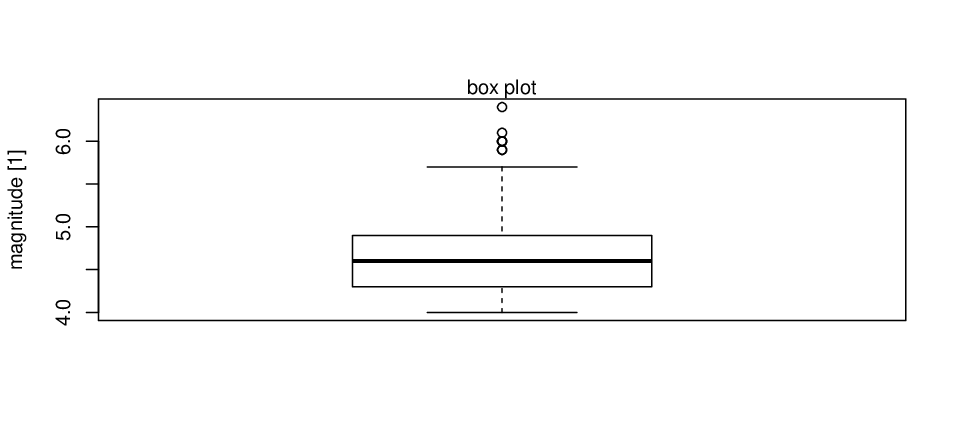
extreme value, if either $x_{i}<\tilde{x}_{0.25}-3d_{Q}$ , or $x_{i}>\tilde{x}_{0.75}+3d_{Q}$ .

A very convenient graphical method for transparently displaying distributional features of metrically scaled data relating to a five number summary, also making explicit the interquartile range, outliers and extreme values, is provided by a box plot; see, e.g., Tukey (1977) [111]. An example of a single box plot is depicted in Fig. 3.1, of parallel box plots in Fig. 3.2.

R: boxplot(variable), boxplot(variable ~ group variable)

3.2.3 Sample variance

The most frequently employed measure of variability in Statistics is the dimensionful $n$ -data-point sample variance $s^{2}$ (metr), and the related sample standard deviation to be discussed below. One of the originators of these concepts is the French mathematician Abraham de Moivre (1667–1754); cf. Bernstein (1998) [4, p 5]. Given a univariate raw data set $\{x_{i}\}_{i=1,\ldots,n}$ for $X$ , its spread is essentially quantified in terms of the sum of squared deviations of the $n$ data points $x_{i}$ from their common sample mean $\bar{x}$ . Due to the algebraic identity

\left(x_{1}-\bar{x}\right)+\ldots+\left(x_{n}-\bar{x}\right)=\sum_{i=1}^{n}\left(x_{i}-\bar{x}\right)=\left(\sum_{i=1}^{n}x_{i}\right)-n\bar{x}\stackrel{{\scriptstyle\text{Eq.}\penalty\ (\ref{eq:arithmean1})}}{{\equiv}}0\ ,

there are only $n-1$ degrees of freedom involved in this measure. The sample variance is thus defined by:

(i)

From a raw data set:

\framebox{$\displaystyle s^{2}:=\frac{1}{n-1}\left[\,(x_{1}-\bar{x})^{2}+\ldots+(x_{n}-\bar{x})^{2}\,\right]=:\frac{1}{n-1}\sum_{i=1}^{n}\left(x_{i}-\bar{x}\right)^{2}\ ;$}

(3.12)

alternatively, by the shift theorem:²² 2 That is, the algebraic identity $\displaystyle\sum_{i=1}^{n}\left(x_{i}-\bar{x}\right)^{2}=\sum_{i=1}^{n}\left(x_{i}^{2}-2x_{i}\bar{x}+\bar{x}^{2}\right)\stackrel{{\scriptstyle\text{Eq.}\penalty\ (\ref{eq:arithmean1})}}{{\equiv}}\sum_{i=1}^{n}x_{i}^{2}-\sum_{i=1}^{n}\bar{x}^{2}=\sum_{i=1}^{n}x_{i}^{2}-n\bar{x}^{2}$ .

s^{2}=\frac{1}{n-1}\left[\,x_{1}^{2}+\ldots+x_{n}^{2}-n\bar{x}{}^{2}\,\right]=\frac{1}{n-1}\left[\,\sum_{i=1}^{n}x_{i}^{2}-n\bar{x}{}^{2}\,\right]\ .

(3.13)

(ii)

From a relative frequency distribution:

	$\displaystyle s^{2}$	$\displaystyle:=$	$\displaystyle\frac{n}{n-1}\left[\,(a_{1}-\bar{x})^{2}h_{n}(a_{1})+\ldots+(a_{k}-\bar{x})^{2}h_{n}(a_{k})\,\right]$		(3.14)
		$\displaystyle=:$	$\displaystyle\frac{n}{n-1}\sum_{j=1}^{k}\left(a_{j}-\bar{x}\right)^{2}h_{n}(a_{j})\ ;$		(3.14)

alternatively:

	$\displaystyle s^{2}$	$\displaystyle=$	$\displaystyle\frac{n}{n-1}\left[\,a_{1}^{2}h_{n}(a_{1})+\ldots+a_{k}^{2}h_{n}(a_{k})-\bar{x}{}^{2}\,\right]$		(3.15)
		$\displaystyle=$	$\displaystyle\frac{n}{n-1}\left[\,\sum_{j=1}^{k}a_{j}^{2}h_{n}(a_{j})-\bar{x}{}^{2}\,\right]\ .$		(3.15)

Remarks: (i) We point out that the alternative formulae for a sample variance provided here prove computationally more efficient.
(ii) For binned data, when one selects the midpoint of each class interval $K_{j}$ to represent the $a_{j}$ (given the raw data set is no longer accessible), a correction of Eqs. (3.14) and (3.15) by an additional term $(1/12)(n/n-1)\sum_{j=1}^{k}b_{j}^{2}h_{j}$ becomes necessary, assuming uniformly distributed data within each of the class intervals $K_{j}$ of width $b_{j}$ ; cf. Eq. (8.41).

R: var(variable)
EXCEL, OpenOffice: VAR.S (dt.: VAR.S, VARIANZ)
SPSS: Analyze $\rightarrow$ Descriptive Statistics $\rightarrow$ Frequencies … $\rightarrow$ Statistics …: Variance

3.2.4 Sample standard deviation

For ease of handling dimensions associated with a metrically scaled one-dimensional variable $X$ , one defines the dimensionful sample standard deviation $s$ (metr) simply as the positive square root of the sample variance (3.12), i.e.,

s:=+\sqrt{s^{2}}\ ,

(3.16)

such that a measure for the spread of data results which shares the dimension of $X$ and its sample mean $\bar{x}$ .

R: sd(variable)
EXCEL, OpenOffice: STDEV.S (dt.: STABW.S, STABW)
SPSS: Analyze $\rightarrow$ Descriptive Statistics $\rightarrow$ Frequencies … $\rightarrow$ Statistics …: Std. deviation

3.2.5 Sample coefficient of variation

For ratio scaled one-dimensional variables $X$ , a dimensionless relative measure of variability is the sample coefficient of variation $v$ (metr: ratio), defined by

v:=\frac{s}{\bar{x}}\ ,\quad\text{if}\quad\bar{x}>0\ .

(3.17)

3.2.6 Standardisation

Data for metrically scaled one-dimensional variables $X$ is amenable to the process of standardisation. By this is meant a linear affine transformation $X\rightarrow Z$ , which generates from a univariate raw data set $\{x_{i}\}_{i=1,\ldots,n}$ of $n$ measured values for a dimensionful variable $X$ , with sample mean $\bar{x}$ and sample standard deviation $s_{X}>0$ , data for an equivalent dimensionless variable $Z$ according to

\framebox{$\displaystyle x_{i}\mapsto z_{i}:=\frac{x_{i}-\bar{x}}{s_{X}}\qquad\text{for all}\ i=1,\ldots,n\ .$}

(3.18)

For the resultant $Z$ -data, referred to as the $\boldsymbol{Z}$ scores of the original metrical $X$ -data, this has the convenient practical consequences that (i) all one-dimensional metrical data is thus represented on the same dimensionless measurement scale, and (ii) the corresponding sample mean and sample standard deviation of the $Z$ -data amount to

\bar{z}=0\quad\text{and}\quad s_{Z}=1\ ,

respectively. Employing Z scores, specific values $x_{i}$ of the original metrical $X$ -data will be expressed in terms of sample standard deviation units, i.e., by how many sample standard deviations they fall on either side of the common sample mean. Essential information on characteristic distributional features of one-dimensional metrical data will be preserved by the process of standardisation.

R: scale(variable, center = TRUE, scale = TRUE)
EXCEL, OpenOffice: STANDARDIZE (dt.: STANDARDISIERUNG)
SPSS: Analyze $\rightarrow$ Descriptive Statistics $\rightarrow$ Descriptives … $\rightarrow$ Save standardized values as variables

3.3 Measures of relative distortion

The third family of measures characterising relative frequency distributions for univariate data $\{x_{i}\}_{i=1,\ldots,n}$ for metrically scaled one-dimensional variables $X$ , having specific sample mean $\bar{x}$ and sample standard deviation $s_{X}$ , relate to the issue of the shape of a distribution. These measures take a Gaußian normal distribution (cf. Sec. 8.6 below) as as a reference case, with the values of its two free parameters equal to the given $\bar{x}$ and $s_{X}$ . With respect to this reference distribution, one defines two kinds of dimensionless measures of relative distortion as described in the following (cf., e.g., Joanes and Gill (1998) [46]).

3.3.1 Skewness

The skewness $g_{1}$ (metr) is a dimensionless measure to quantify the degree of relative distortion of a given frequency distribution in the horizontal direction. Its implementation in the software package EXCEL employs the definition

g_{1}:=\frac{n}{(n-1)(n-2)}\sum_{i=1}^{n}\left(\frac{x_{i}-\bar{x}}{s_{X}}\right)^{3}\qquad\text{for}\quad n>2\ ,

(3.19)

wherein the observed values $\{x_{i}\}_{i=1,\ldots,n}$ enter in their standardised form according to Eq. (3.18). Note that $g_{1}=0$ for an exact Gaußian normal distribution.

R: skewness(variable, type = 2) (package: e1071, by Meyer et al (2019) [72])
EXCEL, OpenOffice: SKEW (dt.: SCHIEFE)
SPSS: Analyze $\rightarrow$ Descriptive Statistics $\rightarrow$ Frequencies … $\rightarrow$ Statistics …: Skewness

3.3.2 Excess kurtosis

The excess kurtosis $g_{2}$ (metr) is a dimensionless measure to quantify the degree of relative distortion of a given frequency distribution in the vertical direction. Its implementation in the software package EXCEL employs the definition

g_{2}:=\frac{n(n+1)}{(n-1)(n-2)(n-3)}\sum_{i=1}^{n}\left(\frac{x_{i}-\bar{x}}{s_{X}}\right)^{4}-\frac{3(n-1)^{2}}{(n-2)(n-3)}\qquad\text{for}\quad n>3\ ,

(3.20)

wherein the observed values $\{x_{i}\}_{i=1,\ldots,n}$ enter in their standardised form according to Eq. (3.18). Note that $g_{2}=0$ for an exact Gaußian normal distribution.

R: kurtosis(variable, type = 2) (package: e1071, by Meyer et al (2019) [72])
EXCEL, OpenOffice: KURT (dt.: KURT)
SPSS: Analyze $\rightarrow$ Descriptive Statistics $\rightarrow$ Frequencies … $\rightarrow$ Statistics …: Kurtosis

3.4 Measures of concentration

Finally, for univariate data $\{x_{i}\}_{i=1,\ldots,n}$ relating to a ratio scaled one-dimensional variable $X$ , which has a discrete spectrum of values $\{a_{j}\}_{j=1,\ldots,k}$ , or which was binned into $k$ different categories $\{K_{j}\}_{j=1,\ldots,k}$ with respective midpoints $a_{j}$ , two kinds of measures of concentration are commonplace in Statistics; one qualitative in nature, the other quantitative.

Begin by defining the total sum for the data $\{x_{i}\}_{i=1,\ldots,n}$ by

S:=\sum_{i=1}^{n}x_{i}=\sum_{j=1}^{k}a_{j}o_{n}(a_{j})\stackrel{{\scriptstyle\text{Eq.}\penalty\ (\ref{eq:arithmean1})}}{{=}}n\bar{x}\ ,

(3.21)

where $(a_{j},o_{n}(a_{j}))_{j=1,\ldots,k}$ is the absolute frequency distribution for the observed values (or categories) of $X$ . Then the relative proportion that the value $a_{j}$ (or the category $K_{j}$ ) takes in $S$ is

\frac{a_{j}o_{n}(a_{j})}{S}=\frac{a_{j}h_{n}(a_{j})}{\bar{x}}\ .

(3.22)

3.4.1 Lorenz curve

From the elements introduced in Eqs. (3.21) and (3.22), the US–American economist Max Otto Lorenz (1876–1959) constructed cumulative relative quantities which constitute the coordinates of a so-called Lorenz curve representing concentration in the distribution for the ratio scaled one-dimensional variable $X$ ; cf. Lorenz (1905) [65]. These coordinates are defined as follows:

•

Horizontal axis:

$k_{i}:=\sum_{j=1}^{i}\frac{o_{n}(a_{j})}{n}=\sum_{j=1}^{i}h_{n}(a_{j})\qquad(i=1,\ldots,k)\ ,$ (3.23)
•

Vertical axis:

$l_{i}:=\sum_{j=1}^{i}\frac{a_{j}o_{n}(a_{j})}{S}=\sum_{j=1}^{i}\frac{a_{j}h_{n}(a_{j})}{\bar{x}}\qquad(i=1,\ldots,k)\ .$ (3.24)

The initial point on a Lorenz curve is generally the coordinate system’s origin, $(k_{0},l_{0})=(0,0)$ , the final point is $(1,1)$ . As a reference facility to measure concentration in the distribution of $X$ in qualitative terms, one defines a null concentration curve as the bisecting line linking $(0,0)$ to $(1,1)$ . The Lorenz curve is interpreted as stating that a point on the curve with coordinates $(k_{i},l_{i})$ represents the fact that $k_{i}\times 100\%$ of the $n$ statistical units take a share of $l_{i}\times 100\%$ in the total sum $S$ for the ratio scaled one-dimensional variable $X$ . Qualitatively, for given univariate data $\{x_{i}\}_{i=1,\ldots,n}$ , the concentration in the distribution of $X$ is the stronger, the larger is the dip of the Lorenz curve relative to the null concentration curve. Note that in addition to the null concentration curve, one can define as a second reference facility a maximum concentration curve such that only the largest value $a_{k}$ (or category $K_{k}$ ) in the spectrum of values of $X$ takes the full share of $100\%$ in the total sum $S$ for $\{x_{i}\}_{i=1,\ldots,n}$ .

3.4.2 Normalised Gini coefficient

The Italian statistician, demographer and sociologist Corrado Gini (1884–1965) devised a quantitative measure for concentration in the distribution for a ratio scaled one-dimensional variable $X$ ; cf. Gini (1921) [34]. The dimensionless normalised Gini coefficient $G_{+}$ (metr: ratio) can be interpreted geometrically as the ratio of areas

G_{+}:=\frac{(\text{area enclosed between Lorenz and null concentration curves})}{(\text{area enclosed between maximum and null concentration curves})}\ .

(3.25)

Its related computational definition is given by

\framebox{$\displaystyle G_{+}:=\frac{n}{n-1}\left[\,\sum_{i=1}^{k}(k_{i-1}+k_{i})\,\frac{a_{i}o_{n}(a_{i})}{S}-1\,\right]\ .$}

(3.26)

Due to normalisation, the range of values is $0\leq G_{+}\leq 1$ . Thus, null concentration amounts to $G_{+}=0$ , while maximum concentration amounts to $G_{+}=1$ .³³ 3 In September 2012 it was reported (implicitly) in the public press that the coordinates underlying the Lorenz curve describing the distribution of private equity in Germany at the time were $(0.00,0.00)$ , $(0.50,0.01)$ , $(0.90,0.50)$ , and $(1.00,1.00)$ ; cf. Ref. [102]. Given that in this case $n\gg 1$ , these values amount to a Gini coefficient of $G_{+}=0.64$ . The Oxfam Report on Wealth Inequality 2019 can be found at the URL (cited on May 31, 2019): www.oxfam.org/en/research/public-good-or-private-wealth.

Chapter 4 Descriptive measures of association for bivariate frequency distributions

Now we come to describe and characterise specific features of bivariate frequency distributions, i.e., intrinsic structures of bivariate raw data sets $\{(x_{i},y_{i})\}_{i=1,\ldots,n}$ obtained from samples $\boldsymbol{S_{\Omega}}$ for a two-dimensional statistical variable $(X,Y)$ from some target population of study objects $\boldsymbol{\Omega}$ . Let us suppose that the spectrum of values resp. categories of $X$ is $a_{1},a_{2},\ldots,a_{k}$ , and the spectrum of values resp. categories of $Y$ is $b_{1},b_{2},\ldots,b_{l}$ , where $k,l\in\mathbb{N}$ . Hence, for the bivariate joint distribution there exists a total of $k\times l$ possible combinations $\{(a_{i},b_{j})\}_{i=1,\ldots,k;j=1,\ldots,l}$ of values resp. categories for $(X,Y)$ . In the following, we will denote associated bivariate absolute (observed) frequencies by $o_{ij}:=o_{n}(a_{i},b_{j})$ , and bivariate relative frequencies by $h_{ij}:=h_{n}(a_{i},b_{j})$ .

4.1 $\boldsymbol{(k\times l)}$ contingency tables

Consider a bivariate raw data set $\{(x_{i},y_{i})\}_{i=1,\ldots,n}$ for a two-dimensional statistical variable $(X,Y)$ , giving rise to $k\times l$ combinations of values resp. categories $\{(a_{i},b_{j})\}_{i=1,\ldots,k;j=1,\ldots,l}$ . The bivariate joint distribution of observed absolute frequencies $o_{ij}$ may be conveniently represented in terms of a $\boldsymbol{(k\times l)}$ contingency table, or cross tabulation, by

\begin{array}[]{c|cccccc|c}o_{ij}&b_{1}&b_{2}&\ldots&b_{j}&\ldots&b_{l}&\Sigma_{j}\\ \hline\cr a_{1}&o_{11}&o_{12}&\ldots&o_{1j}&\ldots&o_{1l}&o_{1+}\\ a_{2}&o_{21}&o_{22}&\ldots&o_{2j}&\ldots&o_{2l}&o_{2+}\\ \vdots&\vdots&\vdots&\ddots&\vdots&\ddots&\vdots&\vdots\\ a_{i}&o_{i1}&o_{i2}&\ldots&o_{ij}&\ldots&o_{il}&o_{i+}\\ \vdots&\vdots&\vdots&\ddots&\vdots&\ddots&\vdots&\vdots\\ a_{k}&o_{k1}&o_{k2}&\ldots&o_{kj}&\ldots&o_{kl}&o_{k+}\\ \hline\cr\Sigma_{i}&o_{+1}&o_{+2}&\ldots&o_{+j}&\ldots&o_{+l}&n\end{array}\ ,

(4.1)

where it holds for all $i=1,\ldots,k$ and $j=1,\ldots,l$ that

0\leq o_{ij}\leq n\qquad\text{and}\qquad\sum_{i=1}^{k}\sum_{j=1}^{l}o_{ij}=n\ .

(4.2)

The corresponding univariate marginal absolute frequencies of $X$ and of $Y$ are

	$\displaystyle o_{i+}$	$\displaystyle:=$	$\displaystyle o_{i1}+o_{i2}+\ldots+o_{ij}+\ldots+o_{il}\ =:\ \sum_{j=1}^{l}o_{ij}$		(4.3)
	$\displaystyle o_{+j}$	$\displaystyle:=$	$\displaystyle o_{1j}+o_{2j}+\ldots+o_{ij}+\ldots+o_{kj}\ =:\ \sum_{i=1}^{k}o_{ij}\ .$		(4.4)

R: CrossTable(row variable, column variable) (package: gmodels, by Warnes et al (2018) [115])
SPSS: Analyze $\rightarrow$ Descriptive Statistics $\rightarrow$ Crosstabs … $\rightarrow$ Cells …: Observed

One obtains the related bivariate joint distribution of observed relative frequencies $h_{ij}$ following the systematics of Eq. (2.2) to yield

\begin{array}[]{c|cccccc|c}h_{ij}&b_{1}&b_{2}&\ldots&b_{j}&\ldots&b_{l}&\Sigma_{j}\\ \hline\cr a_{1}&h_{11}&h_{12}&\ldots&h_{1j}&\ldots&h_{1l}&h_{1+}\\ a_{2}&h_{21}&h_{22}&\ldots&h_{2j}&\ldots&h_{2l}&h_{2+}\\ \vdots&\vdots&\vdots&\ddots&\vdots&\ddots&\vdots&\vdots\\ a_{i}&h_{i1}&h_{i2}&\ldots&h_{ij}&\ldots&h_{il}&h_{i+}\\ \vdots&\vdots&\vdots&\ddots&\vdots&\ddots&\vdots&\vdots\\ a_{k}&h_{k1}&h_{k2}&\ldots&h_{kj}&\ldots&h_{kl}&h_{k+}\\ \hline\cr\Sigma_{i}&h_{+1}&h_{+2}&\ldots&h_{+j}&\ldots&h_{+l}&1\end{array}\ .

(4.5)

Again, it holds for all $i=1,\ldots,k$ and $j=1,\ldots,l$ that

0\leq h_{ij}\leq 1\qquad\text{and}\qquad\sum_{i=1}^{k}\sum_{j=1}^{l}h_{ij}=1\ ,

(4.6)

while the univariate marginal relative frequencies of $X$ and of $Y$ are

	$\displaystyle h_{i+}$	$\displaystyle:=$	$\displaystyle h_{i1}+h_{i2}+\ldots+h_{ij}+\ldots+h_{il}\ =:\ \sum_{j=1}^{l}h_{ij}$		(4.7)
	$\displaystyle h_{+j}$	$\displaystyle:=$	$\displaystyle h_{1j}+h_{2j}+\ldots+h_{ij}+\ldots+h_{kj}\ =:\ \sum_{i=1}^{k}h_{ij}\ .$		(4.8)

On the basis of a $(k\times l)$ contingency table displaying the relative frequencies of the bivariate joint distribution for some two-dimensional variable $(X,Y)$ , one may define two kinds of related conditional relative frequency distributions, namely (i) the conditional distribution of $X$ given $Y$ by

h(a_{i}|b_{j}):=\frac{h_{ij}}{h_{+j}}\ ,

(4.9)

and (ii) the conditional distribution of $Y$ given $X$ by

h(b_{j}|a_{i}):=\frac{h_{ij}}{h_{i+}}\ .

(4.10)

Then, by means of these conditional distributions, a notion of statistical independence of variables $X$ and $Y$ is defined to correspond to the simultaneous properties

h(a_{i}|b_{j})=h(a_{i})=h_{i+}\qquad\text{and}\qquad h(b_{j}|a_{i})=h(b_{j})=h_{+j}\ .

(4.11)

Given these properties hold, it follows from Eqs. (4.9) and (4.10) that

h_{ij}=h_{i+}h_{+j}\ ;

(4.12)

the bivariate relative frequencies $h_{ij}$ in this case are numerically equal to the product of the corresponding univariate marginal relative frequencies $h_{i+}$ and $h_{+j}$ .

4.2 Measures of association for the metrical scale level

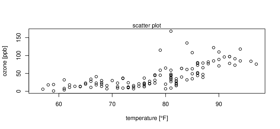
Next, specifically consider a bivariate raw data set $\{(x_{i},y_{i})\}_{i=1,\ldots,n}$ from a statistical sample $\boldsymbol{S_{\Omega}}$ for a metrically scaled two-dimensional variable $(X,Y)$ . The bivariate joint distribution for $(X,Y)$ in this sample can be conveniently represented graphically in terms of a scatter plot, cf. Fig. 4.1, thus uniquely locating the positions of $n$ sampling units in (a subset of) Euclidian space $\mathbb{R}^{2}$ . Let us now introduce two kinds of measures for the description of specific characteristic features of such bivariate joint distributions.

R: plot(variable1, variable2)

4.2.1 Sample covariance

The first standard measure describing degree of association in the joint distribution for a metrically scaled two-dimensional variable $(X,Y)$ is the dimensionful sample covariance $s_{XY}$ (metr), defined by

(i)

From a raw data set:

	$\displaystyle s_{XY}$	$\displaystyle:=$	$\displaystyle\frac{1}{n-1}\left[\,(x_{1}-\bar{x})(y_{1}-\bar{y})+\ldots+(x_{n}-\bar{x})(y_{n}-\bar{y})\,\right]$		(4.13)
		$\displaystyle=:$	$\displaystyle\frac{1}{n-1}\sum_{i=1}^{n}\left(x_{i}-\bar{x}\right)\left(y_{i}-\bar{y}\right)\ ;$		(4.13)

alternatively:

	$\displaystyle s_{XY}$	$\displaystyle=$	$\displaystyle\frac{1}{n-1}\left[\,x_{1}y_{1}+\ldots+x_{n}y_{n}-n\bar{x}\bar{y}\,\right]$		(4.14)
		$\displaystyle=$	$\displaystyle\frac{1}{n-1}\left[\,\sum_{i=1}^{n}x_{i}y_{i}-n\bar{x}\bar{y}\,\right]\ .$		(4.14)

(ii)

From a relative frequency distribution:

	$\displaystyle s_{XY}$	$\displaystyle:=$	$\displaystyle\frac{n}{n-1}\left[\,(a_{1}-\bar{x})(b_{1}-\bar{y})h_{11}+\ldots+(a_{k}-\bar{x})(b_{l}-\bar{y})h_{kl}\,\right]$		(4.15)
		$\displaystyle=:$	$\displaystyle\frac{n}{n-1}\sum_{i=1}^{k}\sum_{j=1}^{l}\left(a_{i}-\bar{x}\right)\left(b_{j}-\bar{y}\right)h_{ij}\ ;$		(4.15)

alternatively:

	$\displaystyle s_{XY}$	$\displaystyle=$	$\displaystyle\frac{n}{n-1}\left[\,a_{1}b_{1}h_{11}+\ldots+a_{k}b_{l}h_{kl}-\bar{x}\bar{y}\,\right]$		(4.16)
		$\displaystyle=$	$\displaystyle\frac{n}{n-1}\left[\,\sum_{i=1}^{k}\sum_{j=1}^{l}a_{i}b_{j}h_{ij}-\bar{x}\bar{y}\,\right]\ .$		(4.16)

Remark: The alternative formulae provided here prove computationally more efficient.

R: cov(variable1, variable2)
EXCEL, OpenOffice: COVARIANCE.S (dt.: KOVARIANZ.S, KOVAR)

In view of its defining equation (4.13), the sample covariance can be given the following geometrical interpretation. For a total of $n$ data points $(x_{i},y_{i})$ , it quantitfies the degree of excess of signed rectangular areas $\left(x_{i}-\bar{x}\right)\left(y_{i}-\bar{y}\right)$ with respect to the common centroid ${\displaystyle\boldsymbol{r}_{C}:=\left(\begin{array}[]{c}\bar{x}\\ \bar{y}\end{array}\right)}$ of the $n$ data points in favour of either positive or negative signed areas, if any.¹¹ 1 The centroid is the special case of equal mass points, with masses $m_{i}=\frac{1}{n}$ , of the centre of gravity of a system of $n$ discrete massive objects, defined by ${\displaystyle\boldsymbol{r}_{C}:=\frac{\sum_{i=1}^{n}m_{i}\boldsymbol{r}_{i}}{\sum_{j=1}^{n}m_{j}}}$ . In two Euclidian dimensions the position vector is ${\displaystyle\boldsymbol{r}_{i}=\left(\begin{array}[]{c}x_{i}\\ y_{i}\end{array}\right)}$ .

It is worthwhile to point out that in the research literature it is standard to define for the joint distribution for a metrically scaled two-dimensional variable $(X,Y)$ a dimensionful symmetric $\boldsymbol{(2\times 2)}$ sample covariance matrix $\boldsymbol{S^{2}}$ according to

\boldsymbol{S^{2}}:=\left(\begin{array}[]{cc}s_{X}^{2}&s_{XY}\\ s_{XY}&s_{Y}^{2}\end{array}\right)\ ,

(4.17)

the components of which are defined by Eqs. (3.12) and (4.13). The determinant of $\boldsymbol{S^{2}}$ , given by $\det(\boldsymbol{S^{2}})=s_{X}^{2}s_{Y}^{2}-s_{XY}^{2}$ , is positive as long as $s_{X}^{2}s_{Y}^{2}-s_{XY}^{2}>0$ , which applies in most practical cases. Then $\boldsymbol{S^{2}}$ is regular, and thus a corresponding inverse $(\boldsymbol{S^{2}})^{-1}$ exists; cf. Ref. [19, Sec. 3.5].

The concept of a regular sample covariance matrix $\boldsymbol{S^{2}}$ and its inverse $(\boldsymbol{S^{2}})^{-1}$ generalises in a straightforward fashion to the case of multivariate joint distributions for metrically scaled $m$ -dimensional statistical variables $(X,Y,\ldots,Z)$ , where $\boldsymbol{S^{2}}\in\mathbb{R}^{m\times m}$ is given by

\boldsymbol{S^{2}}:=\left(\begin{array}[]{cccc}s_{X}^{2}&s_{XY}&\ldots&s_{ZX}\\ s_{XY}&s_{Y}^{2}&\ldots&s_{YZ}\\ \vdots&\vdots&\ddots&\vdots\\ s_{ZX}&s_{YZ}&\ldots&s_{Z}^{2}\end{array}\right)\ ,

(4.18)

and $\det(\boldsymbol{S^{2}})\neq 0$ is required.

4.2.2 Bravais and Pearson’s sample correlation coefficient

The sample covariance $s_{XY}$ constitutes the basis for the second standard measure characterising the joint distribution for a metrically scaled two-dimensional variable $(X,Y)$ by descriptive means, which is the normalised and dimensionless sample correlation coefficient $r$ (metr) devised by the French physicist Auguste Bravais (1811–1863) and the English mathematician and statistician Karl Pearson FRS (1857–1936) for the purpose of analysing corresponding bivariate raw data $\{(x_{i},y_{i})\}_{i=1,\ldots,n}$ for the existence of a linear (!!!) statistical association. It is defined in terms of the bivariate sample covariance $s_{XY}$ and the univariate sample standard deviations $s_{X}$ and $s_{Y}$ by (cf. Bravais (1846) [9] and Pearson (1901, 1920) [80, 82])

\framebox{$\displaystyle r:=\frac{s_{XY}}{s_{X}s_{Y}}\ .$}

(4.19)

With Eq. (4.13) for $s_{XY}$ , this becomes

r=\frac{1}{n-1}\sum_{i=1}^{n}\left(\frac{x_{i}-\bar{x}}{s_{X}}\right)\left(\frac{y_{i}-\bar{y}}{s_{Y}}\right)=\frac{1}{n-1}\sum_{i=1}^{n}z_{i}^{X}z_{i}^{Y}\ ,

(4.20)

employing standardisation according to Eq. (3.18) in the final step. Due to its normalisation, the range of the sample correlation coefficient is $-1\leq r\leq+1$ . The sign of $r$ encodes the direction of a correlation. As to interpreting the strength of a correlation via the magnitude $|r|$ , in practice one typically employs the following qualitative

Rule of thumb:
$0.0=|r|$ : no correlation
$0.0<|r|<0.2$ : very weak correlation
$0.2\leq|r|<0.4$ : weak correlation
$0.4\leq|r|<0.6$ : moderately strong correlation
$0.6\leq|r|\leq 0.8$ : strong correlation
$0.8\leq|r|<1.0$ : very strong correlation
$1.0=|r|$ : perfect correlation.

R: cor(variable1, variable2)
EXCEL, OpenOffice: CORREL (dt.: KORREL)
SPSS: Analyze $\rightarrow$ Correlate $\rightarrow$ Bivariate …: Pearson

In line with Eq. (4.17), it is convenient to define a dimensionless symmetric $\boldsymbol{(2\times 2)}$ sample correlation matrix $\boldsymbol{R}$ by

\boldsymbol{R}:=\left(\begin{array}[]{cc}1&r\\ r&1\end{array}\right)\ ,

(4.21)

which is regular and positive definite as long as its determinant $\det(\boldsymbol{R})=1-r^{2}>0$ . In this case, its inverse $\boldsymbol{R}^{-1}$ is given by

\boldsymbol{R}^{-1}=\frac{1}{1-r^{2}}\left(\begin{array}[]{rr}1&-r\\ -r&1\end{array}\right)\ .

(4.22)

Note that for non-correlating metrically scaled variables $X$ and $Y$ , i.e., when $r=0$ , the sample correlation matrix degenerates to become a unit matrix, $\boldsymbol{R}=\boldsymbol{1}$ .

Again, the concept of a regular and positive definite sample correlation matrix $\boldsymbol{R}$ , with inverse $\boldsymbol{R}^{-1}$ , generalises to multivariate joint distributions for metrically scaled $m$ -dimensional statistical variables $(X,Y,\ldots,Z)$ , where $\boldsymbol{R}\in\mathbb{R}^{m\times m}$ is given by²² 2 Given a data matrix $\boldsymbol{X}\in\mathbb{R}^{n\times m}$ for a metrically scaled $m$ -dimensional statistical variable $(X,Y,\ldots,Z)$ , one can show that upon standardisation of the data according to Eq. (3.18), which amounts to a transformation $\boldsymbol{X}\mapsto\boldsymbol{Z}\in\mathbb{R}^{n\times m}$ , the sample correlation matrix can be represented by $\displaystyle\boldsymbol{R}=\frac{1}{n-1}\,\boldsymbol{Z}^{T}\boldsymbol{Z}$ . The form of this relation is equivalent to Eq. (4.20).

\boldsymbol{R}:=\left(\begin{array}[]{cccc}1&r_{XY}&\ldots&r_{ZX}\\ r_{XY}&1&\ldots&r_{YZ}\\ \vdots&\vdots&\ddots&\vdots\\ r_{ZX}&r_{YZ}&\ldots&1\end{array}\right)\ ,

(4.23)

and $\det(\boldsymbol{R})\neq 0$ . Note that $\boldsymbol{R}$ is a dimensionless quantity which, hence, is scale-invariant; cf. Sec. 8.10.

4.3 Measures of association for the ordinal scale level

At the ordinal scale level, bivariate raw data $\{(x_{i},y_{i})\}_{i=1,\ldots,n}$ for a two-dimensional variable $(X,Y)$ is not necessarily quantitative in nature. Therefore, in order to be in a position to define a sensible quantitative bivariate measure of statistical association for ordinal variables, one needs to introduce meaningful surrogate data which is numerical. This task is realised by means of defining so-called rank numbers, which are assigned to the original ordinal data according to the procedure described in the following.

Begin by establishing amongst the observed values $\{x_{i}\}_{i=1,\ldots,n}$ resp. $\{y_{i}\}_{i=1,\ldots,n}$ their natural ascending rank order, i.e.,

x_{(1)}\leq x_{(2)}\leq\ldots\leq x_{(n)}\qquad\text{and}\qquad y_{(1)}\leq y_{(2)}\leq\ldots\leq y_{(n)}\ .

(4.24)

Then, every individual $x_{i}$ resp. $y_{i}$ is assigned a rank number which corresponds to its position in the ordered sequences (4.24):

x_{i}\mapsto R(x_{i})\ ,\quad y_{i}\mapsto R(y_{i})\ ,\quad\quad\text{for all}\quad i=1,\ldots,n\ .

(4.25)

Should there be any “tied ranks” due to equality of some $x_{i}$ or $y_{i}$ , one assigns the arithmetical mean of the corresponding rank numbers to all $x_{i}$ resp. $y_{i}$ involved in the “tie.” Ultimately, by this procedure, the entire bivariate raw data undergoes a transformation

\{(x_{i},y_{i})\}_{i=1,\ldots,n}\mapsto\{[R(x_{i}),R(y_{i})]\}_{i=1,\ldots,n}\ ,

(4.26)

yielding $n$ pairs of rank numbers to numerically represent the original bivariate ordinal data.

Given surrogate rank number data, the means of rank numbers always amount to

	$\displaystyle\bar{R}(x)$	$\displaystyle:=$	$\displaystyle\frac{1}{n}\sum_{i=1}^{n}R(x_{i})\ =\ \frac{n+1}{2}$		(4.27)
	$\displaystyle\bar{R}(y)$	$\displaystyle:=$	$\displaystyle\frac{1}{n}\sum_{i=1}^{n}R(y_{i})\ =\ \frac{n+1}{2}\ .$		(4.28)

The variances of rank numbers are defined in accordance with Eqs. (3.13) and (3.15), i.e.,

	$\displaystyle s_{R(x)}^{2}$	$\displaystyle:=$	$\displaystyle\frac{1}{n-1}\,\left[\,\sum_{i=1}^{n}R^{2}(x_{i})-n\bar{R}^{2}(x)\,\right]\ =\ \frac{n}{n-1}\,\left[\,\sum_{i=1}^{k}R^{2}(a_{i})h_{i+}-\bar{R}^{2}(x)\,\right]$		(4.29)
	$\displaystyle s_{R(y)}^{2}$	$\displaystyle:=$	$\displaystyle\frac{1}{n-1}\,\left[\,\sum_{i=1}^{n}R^{2}(y_{i})-n\bar{R}^{2}(y)\,\right]\ =\ \frac{n}{n-1}\,\left[\,\sum_{j=1}^{l}R^{2}(b_{j})h_{+j}-\bar{R}^{2}(y)\,\right]\ .$		(4.30)

In addition, to characterise the joint distribution of rank numbers, a sample covariance of rank numbers is defined in line with Eqs. (4.14) and (4.16) by

	$\displaystyle s_{R(x)R(y)}$	$\displaystyle:=$	$\displaystyle\frac{1}{n-1}\,\left[\,\sum_{i=1}^{n}R(x_{i})R(y_{i})-n\bar{R}(x)\bar{R}(y)\,\right]$		(4.31)
		$\displaystyle=$	$\displaystyle\frac{n}{n-1}\,\left[\,\sum_{i=1}^{k}\sum_{j=1}^{l}R(a_{i})R(b_{j})h_{ij}-\bar{R}(x)\bar{R}(y)\,\right]\ .$		(4.31)

On this fairly elaborate technical backdrop, the English psychologist and statistician Charles Edward Spearman FRS (1863–1945) defined a dimensionless sample rank correlation coefficient $r_{S}$ (ord), in analogy to Eq. (4.19), by (cf. Spearman (1904) [97])

\framebox{$\displaystyle r_{S}:=\frac{s_{R(x)R(y)}}{s_{R(x)}s_{R(y)}}\ .$}

(4.32)

The range of this rank correlation coefficient is $-1\leq r_{S}\leq+1$ . Again, while the sign of $r_{S}$ encodes the direction of a rank correlation, in interpreting the strength of a rank correlation via the magnitude $|r_{S}|$ one usually employs the qualitative

Rule of thumb:
$0.0=|r_{S}|$ : no rank correlation
$0.0<|r_{S}|<0.2$ : very weak rank correlation
$0.2\leq|r_{S}|<0.4$ : weak rank correlation
$0.4\leq|r_{S}|<0.6$ : moderately strong rank correlation
$0.6\leq|r_{S}|\leq 0.8$ : strong rank correlation
$0.8\leq|r_{S}|<1.0$ : very strong rank correlation
$1.0=|r_{S}|$ : perfect rank correlation.

R: cor(variable1, variable2, method = "spearman")
SPSS: Analyze $\rightarrow$ Correlate $\rightarrow$ Bivariate …: Spearman

When no tied ranks occur, Eq. (4.32) simplifies to (cf. Hartung et al (2005) [40, p 554])

r_{S}=1-\frac{6\sum_{i=1}^{n}[R(x_{i})-R(y_{i})]^{2}}{n(n^{2}-1)}\ .

(4.33)

4.4 Measures of association for the nominal scale level

Lastly, let us turn to consider the case of quantifying the degree of statistical association in bivariate raw data $\{(x_{i},y_{i})\}_{i=1,\ldots,n}$ for a nominally scaled two-dimensional variable $(X,Y)$ , with categories $\{(a_{i},b_{j})\}_{i=1,\ldots,k;j=1,\ldots,l}$ . The starting point are the observed bivariate absolute resp. relative (cell) frequencies $o_{ij}$ and $h_{ij}$ of the joint distribution for $(X,Y)$ , with univariate marginal frequencies $o_{i+}$ resp. $h_{i+}$ for $X$ and $o_{+j}$ resp. $h_{+j}$ for $Y$ . The $\boldsymbol{\chi}^{2}$ –statistic devised by the English mathematical statistician Karl Pearson FRS (1857–1936) rests on the notion of statistical independence of two one-dimensional variables $X$ and $Y$ in that it takes the corresponding formal condition provided by Eq. (4.12) as a reference state. A simple algebraic manipulation of this condition obtains

h_{ij}=h_{i+}h_{+j}\quad\Rightarrow\quad\frac{o_{ij}}{n}=\frac{o_{i+}}{n}\,\frac{o_{+j}}{n}\quad\overbrace{\Rightarrow}^{\text{multiplication by}\ n}\quad o_{ij}=\frac{o_{i+}o_{+j}}{n}\ .

(4.34)

Pearson’s descriptive $\chi^{2}$ –statistic (cf. Pearson (1900) [79]) is then defined by

\framebox{$\displaystyle\chi^{2}:=\sum_{i=1}^{k}\sum_{j=1}^{l}\frac{\left(o_{ij}-{\displaystyle\frac{o_{i+}o_{+j}}{n}}\right)^{2}}{{\displaystyle\frac{o_{i+}o_{+j}}{n}}}=n\sum_{i=1}^{k}\sum_{j=1}^{l}\frac{\left(h_{ij}-h_{i+}h_{+j}\right)^{2}}{h_{i+}h_{+j}}\ ,$}

(4.35)

whose range of values amounts to $0\leq\chi^{2}\leq\max(\chi^{2})$ , with $\max(\chi^{2}):=n\,[\min(k,l)-1]$ .

Remark: Provided $\displaystyle\frac{o_{i+}o_{+j}}{n}\geq 5$ for all $i=1,\ldots,k$ and $j=1,\ldots,l$ , Pearson’s $\chi^{2}$ –statistic can be employed for the analysis of statistical associations amongst the components of a two-dimensional variable $(X,Y)$ of almost all combinations of scale levels.

The problem with Pearson’s $\chi^{2}$ –statistic is that, due to its variable spectrum of values, it is not immediately clear how to use it efficiently in interpreting the strength of statistical associations. This shortcoming can, however, be overcome by resorting to the measure of association proposed by the Swedish mathematician, actuary, and statistician Carl Harald Cramér (1893–1985), which basically is the result of a special kind of normalisation of Pearson’s measure. Thus, Cramér’s $\boldsymbol{V}$ , as it has come to be known, is defined by (cf. Cramér (1946) [14])

\framebox{$\displaystyle V:=\sqrt{\frac{\chi^{2}}{\max(\chi^{2})}}\ ,$}

(4.36)

with range $0\leq V\leq 1$ . For the interpretation of the strength of statistical association in the joint distribution for a two-dimensional categorical variable $(X,Y)$ , one may thus employ the qualitative

Rule of thumb:
$0.0\leq V<0.2$ : weak association
$0.2\leq V<0.6$ : moderately strong association
$0.6\leq V\leq 1.0$ : strong association.

R: assocstats(contingency table) (package: vcd, by Meyer et al (2017) [71])
SPSS: Analyze $\rightarrow$ Descriptive Statistics $\rightarrow$ Crosstabs … $\rightarrow$ Statistics …: Chi-square, Phi and Cramer’s V

Chapter 5 Descriptive linear regression analysis

For strongly correlating bivariate sample data $\{(x_{i},y_{i})\}_{i=1,\ldots,n}$ for a metrically scaled two-dimensional statistical variable $(X,Y)$ , i.e., when $0.71\leq|r|\leq 1.0$ , it is meaningful to construct a mathematical model of the linear quantitative statistical association so diagnosed. The standard method to realise this by systematic means is due to the German mathematician and astronomer Carl Friedrich Gauß (1777–1855) and is known by the name of descriptive linear regression analysis; cf. Gauß (1809) [30]. We here restrict our attention to the case of simple linear regression, which aims to explain the variability in one dependent variable in terms of the variability in a single independent variable.

To be determined is a best-fit linear model to given bivariate metrical data $\{(x_{i},y_{i})\}_{i=1,\ldots,n}$ . The linear model in question can be expressed in mathematical terms by

\framebox{$\displaystyle\hat{y}=a+bx\ ,$}

(5.1)

with unknown regression coefficients $\boldsymbol{y}$ -intercept $a$ and slope $b$ . Gauß’ method of least squares works as follows.

5.1 Method of least squares

At first, one has to make a choice: assign $X$ the status of an independent variable, and $Y$ the status of a dependent variable (or vice versa; usually this freedom of choice does exist, unless one is testing a specific functional or suspected causal relationship, $y=f(x)$ ). Then, considering the measured values $x_{i}$ for $X$ as fixed, to be minimised for the $Y$ -data is the sum of the squared vertical deviations of the measured values $y_{i}$ from the model values $\hat{y}_{i}=a+bx_{i}$ . The latter are associated with an arbitrary straight line through the cloud of data points $\{(x_{i},y_{i})\}_{i=1,\ldots,n}$ in a scatter plot. This sum, given by

S(a,b):=\sum_{i=1}^{n}(y_{i}-\hat{y}_{i})^{2}=\sum_{i=1}^{n}(y_{i}-a-bx_{i})^{2}\ ,

(5.2)

constitutes a non-negative real-valued function of two variables, $a$ and $b$ . Hence, determining its (local) minimum values entails satisfying (i) the necessary condition of simultaneously vanishing first partial derivatives

0\stackrel{{\scriptstyle!}}{{=}}\frac{\partial S(a,b)}{\partial a}\ ,\qquad 0\stackrel{{\scriptstyle!}}{{=}}\frac{\partial S(a,b)}{\partial b}\ ,

(5.3)

— this yields a well-determined $(2\times 2)$ system of linear algebraic equations for the unknowns $a$ and $b$ , cf. Ref. [19, Sec. 3.1] —, and (ii) the sufficient condition of a positive definite Hessian matrix $H(a,b)$ of second partial derivatives,

H(a,b):=\left(\begin{array}[]{ccc}{\displaystyle\frac{\partial^{2}S(a,b)}{\partial a^{2}}}&&{\displaystyle\frac{\partial^{2}S(a,b)}{\partial a\partial b}}\\ \\ {\displaystyle\frac{\partial^{2}S(a,b)}{\partial b\partial a}}&&{\displaystyle\frac{\partial^{2}S(a,b)}{\partial b^{2}}}\end{array}\right)\ ,

(5.4)

at the candidate optimal values of $a$ and $b$ . $H(a,b)$ is referred to as positive definite when all of its eigenvalues are positive; cf. Ref. [19, Sec. 3.6].

5.2 Empirical regression line

It is a fairly straightforward algebraic exercise (see, e.g., Toutenburg (2004) [108, p 141ff]) to show that the values of the unknowns $a$ and $b$ , which determine a unique global minimum of $S(a,b)$ , amount to

\framebox{$\displaystyle b=\frac{s_{Y}}{s_{X}}\,r\ ,\qquad a=\bar{y}-b\bar{x}\ .$}

(5.5)

These values are referred to as the least squares estimators for $a$ and $b$ . Note that they are exclusively expressible in terms of familiar univariate and bivariate measures characterising the joint distribution for $(X,Y)$ .

With the solutions $a$ and $b$ of Eq. (5.5) inserted in Eq. (5.1), the resultant best-fit linear model is given by

\framebox{$\displaystyle\hat{y}=\bar{y}+\frac{s_{Y}}{s_{X}}\,r\,(x-\bar{x})\ .$}

(5.6)

It may be employed for the purpose of generating intrapolating predictions of the kind $x\mapsto\hat{y}$ , for $x$ -values confined to the empirical interval $[x_{(1)},x_{(n)}]$ . An example of a best-fit linear model obtained by the method of least squares is shown in Fig. 5.1.

R: lm(variable:y ~ variable:x)
EXCEL, OpenOffice: SLOPE, INTERCEPT (dt.: STEIGUNG, ACHSENABSCHNITT)
SPSS: Analyze $\rightarrow$ Regression $\rightarrow$ Linear …

Note that Eq. (5.6) may be re-expressed in terms of the corresponding $Z$ scores of $X$ and $\hat{Y}$ , according to Eq. (3.18). This yields

\left(\frac{\hat{y}-\bar{y}}{s_{Y}}\right)=r\left(\frac{x-\bar{x}}{s_{X}}\right)\qquad\Leftrightarrow\qquad\hat{z}_{Y}=rz_{X}\ .

(5.7)

5.3 Coefficient of determination

The quality of any particular simple linear regression model, i.e., its goodness-of-the-fit, is assessed by means of the coefficient of determination $B$ (metr). This measure is derived by starting from the algebraic identity

\sum_{i=1}^{n}(y_{i}-\bar{y})^{2}=\sum_{i=1}^{n}(\hat{y}_{i}-\bar{y})^{2}+\sum_{i=1}^{n}(y_{i}-\hat{y}_{i})^{2}\ ,

(5.8)

which, upon conveniently re-arranging, leads to defining a quantity

\framebox{$\displaystyle B:=\frac{{\displaystyle\sum_{i=1}^{n}(y_{i}-\bar{y})^{2}-\sum_{i=1}^{n}(y_{i}-\hat{y}_{i})^{2}}}{{\displaystyle\sum_{i=1}^{n}(y_{i}-\bar{y})^{2}}}=\frac{{\displaystyle\sum_{i=1}^{n}(\hat{y}_{i}-\bar{y})^{2}}}{{\displaystyle\sum_{i=1}^{n}(y_{i}-\bar{y})^{2}}}\ ,$}

(5.9)

with range $0\leq B\leq 1$ . A perfect fit is signified by $B=1$ , while no fit amounts to $B=0$ . The coefficient of determination provides a descriptive measure for the proportion of variability of $Y$ in a bivariate data set $\{(x_{i},y_{i})\}_{i=1,\ldots,n}$ that can be accounted for as due to the association with $X$ via the simple linear regression model. Note that in simple linear regression it holds that

B=r^{2}\ ;

(5.10)

see, e.g., Toutenburg (2004) [108, p 150f]).

R: summary( lm(variable:y ~ variable:x) )
EXCEL, OpenOffice: RSQ (dt.: BESTIMMTHEITSMASS)
SPSS: Analyze $\rightarrow$ Regression $\rightarrow$ Linear … $\rightarrow$ Statistics …: Model fit

This concludes Part I of these lecture notes, the introductory discussion on uni- and bivariate descriptive statistical methods of data analysis. We wish to encourage the interested reader to adhere to accepted scientific standards when actively getting involved with data analysis her/him-self. This entails, amongst other aspects, foremost the truthful documentation of all data taken into account in a specific analysis conducted. Features facilitating understanding such as visualisations of empirical distributions by means of, where appropriate, histograms, bar charts, box plots or scatter plots, or providing the values of five number summaries, sample means, sample standard deviations, standardised skewness and excess kurtosis measures, or sample correlation coefficients should be commonplace in any kind of research report. It must be a prime objective of the researcher to empower potential readers to retrace the inferences made by her/him.

To set the stage for the application of inferential statistical methods in Part III, we now turn to review the elementary concepts underlying Probability Theory, predominantly as interpreted in the frequentist approach to this topic.

Chapter 6 Elements of probability theory

All examples of inferential statistical methods of data analysis to be presented in Chs. 12 and 13 have been developed in the context of the so-called frequentist approach to Probability Theory.¹¹ 1 The origin of the term “probability” is traced back to the Latin word probabilis, which the Roman philosopher Cicero (106 BC–43 BC) used to capture a notion of plausibility or likelihood; see Mlodinow (2008) [74, p 32]. The issue in Inferential Statistics is to estimate the plausibility or likelihood of hypotheses given the observational evidence for them. The frequentist approach was pioneered by the Italian mathematician, physician, astrologer, philosopher and gambler Girolamo Cardano (1501–1576), the French lawyer and amateur mathematician Pierre de Fermat (1601–1665), the French mathematician, physicist, inventor, writer and Catholic philosopher Blaise Pascal (1623–1662), the Swiss mathematician Jakob Bernoulli (1654–1705), and the French mathematician and astronomer Marquis Pierre Simon de Laplace (1749–1827). It is deeply rooted in the two fundamental assumptions that any particular random experiment can be repeated arbitrarily often (i) under the “same conditions,” and (ii) completely “independent of one another,” so that a theoretical basis is given for defining allegedly “objective probabilities” for random events and hypotheses via the relative frequencies of very long sequences of repetition of the same random experiment.²² 2 A special role in the context of the frequentist approach to Probability Theory is assumed by Jakob Bernoulli’s law of large numbers, as well as the concept of independently and identically distributed (in short: “i.i.d.”) random variables; we will discuss these issues in Sec. 8.15 below. This is a highly idealised viewpoint, however, which shares only a limited degree of similarity with the actual conditions pertaining to an observer’s resp. experimentor’s reality. Renowned textbooks adopting the frequentist viewpoint of Probability Theory and Inferential Statistics are, e.g., Cramér (1946) [14] and Feller (1968) [22].

Not everyone in Statistics is entirely happy, though, with the philosophy underlying the frequentist approach to introducing the concept of probability, as a number of its central ideas rely on unobserved data (information). A complementary viewpoint is taken by the framework which originated from the work of the English mathematician and Presbyterian minister Thomas Bayes (1702–1761), and later of Laplace, and so is commonly referred to as the Bayes–Laplace approach; cf. Bayes (1763) [3] and Laplace (1812) [59]. A striking conceptual difference to the frequentist approach consists in its use of prior, allegedly “subjective probabilities” for random events and hypotheses, quantifying a persons’s individual reasonable degree-of-belief in their likelihood, which are subsequently updated by analysing relevant empirical data.³³ 3 Anscombe and Aumann (1963) [2] in their seminal paper refer to “objective probabilities” as associated with “roulette lotteries,” and to “subjective probabilities” as associated with “horse lotteries.” Savage (1954) [90] employs the alternative terminology of distinguishing between “objectivistic probabilities” and “personalistic probabilities.” Renowned textbooks adopting the Bayes–Laplace viewpoint of Probability Theory and Inferential Statistics are, e.g., Jeffreys (1939) [45] and Jaynes (2003) [44], while general information regarding the Bayes–Laplace approach is available from the website bayes.wustl.edu. More recent textbooks, which assist in the implementation of advanced computational routines, have been issued by Gelman et al (2014) [31] and by McElreath (2016) [70]. A discussion of the pros and cons of either of these two competing approaches to Probability Theory can be found, e.g., in Sivia and Skilling (2006) [93, p 8ff], or in Gilboa (2009) [32, Sec. 5.3].

A common denominator of both frameworks, frequentist and Bayes–Laplace, is the attempt to quantify a notion of uncertainty that can be related to in formal treatments of decision-making. In the following we turn to discuss the general principles on which Probability Theory is built.

6.1 Random events

We begin by introducing some basic formal constructions and corresponding terminology used in the frequentist approach to Probability Theory:

•

Random experiments: Random experiments are experiments which can be repeated arbitrarily often under identical conditions, with events — also called outcomes — that cannot be predicted with certainty. Well-known simple examples are found amongst games of chance such as tossing a coin, rolling dice, or playing roulette.
•
Sample space $\boldsymbol{\Omega}=\{\omega_{1},\omega_{2},\ldots\}$ : The sample space associated with a random experiment is constituted by the set of all possible elementary events (or elementary outcomes) $\omega_{i}$ ( $i=1,2,\ldots$ ), which are signified by their property of mutual exclusivity. The sample space $\boldsymbol{\Omega}$ of a random experiment may contain either
- (i)
  
  a finite number $n$ of elementary events; then $|\boldsymbol{\Omega}|=n$ , or
- (ii)
  
  countably many elementary events in the sense of a one-to-one correspondence with the set of natural numbers $\mathbb{N}$ , or
- (iii)
  
  uncountably may elements in the sense of a one-to-one correspondence with the set of real numbers $\mathbb{R}$ , or an open or closed subset thereof.⁴⁴ 4 For reasons of definiteness, we will assume in this case that the sample space $\boldsymbol{\Omega}$ associated with a random experiment is compact.
The essential concept of the sample space associated with a random experiment was introduced to Probability Theory by the Italian mathematician Girolamo Cardano (1501–1576); see Cardano (1564) [11], Mlodinow (2008) [74, p 42], and Bernstein (1998) [4, p 47ff].
•

Random events $A,B,\ldots\subseteq\boldsymbol{\Omega}$ : Random events are formally defined as all kinds of subsets of $\boldsymbol{\Omega}$ that can be formed from the elementary events $\omega_{i}\in\boldsymbol{\Omega}$ .
•

Certain event $\boldsymbol{\Omega}$ : The certain event is synonymous with the sample space itself. When a particular random experiment is conducted, “something will happen for sure.”
•

Impossible event $\emptyset=\{\}=\bar{\boldsymbol{\Omega}}$ : The impossible event is the natural complement to the certain event. When a particular random experiment is conducted, “it is not possible that nothing will happen at all.”
•

Event space ${\cal P}(\boldsymbol{\Omega}):=\{A|A\subseteq\boldsymbol{\Omega}\}$ : The event space, also referred to as the power set of $\boldsymbol{\Omega}$ , is the set of all possible subsets (random events!) that can be formed from elementary events $\omega_{i}\in\boldsymbol{\Omega}$ . Its size (or cardinality) is given by $|{\cal P}(\boldsymbol{\Omega})|=2^{|\boldsymbol{\Omega}|}$ . The event space ${\cal P}(\boldsymbol{\Omega})$ constitutes a so-called $\boldsymbol{\sigma}$ –algebra associated with the sample space $\boldsymbol{\Omega}$ ; cf. Rinne (2008) [88, p 177]. When $|\boldsymbol{\Omega}|=n$ , i.e., when $\boldsymbol{\Omega}$ is finite, then $|{\cal P}(\boldsymbol{\Omega})|=2^{n}$ .

In the formulation of probability theoretical laws and computational rules, the following set operations and identities prove useful.

Set operations

1.

$\bar{A}=\boldsymbol{\Omega}\backslash A$ — complementation of a set (or event) $A$ (“not $A$ ”)
2.

$A\backslash B=A\cap\bar{B}$ — formation of the difference of sets (or events) $A$ and $B$ (“ $A$ , but not $B$ ”)
3.

$A\cup B$ — formation of the union of sets (or events) $A$ and $B$ , otherwise referred to as the disjunction of $A$ and $B$ (“ $A$ or $B$ ”)
4.

$A\cap B$ — formation of the intersection of sets (or events) $A$ and $B$ , otherwise referred to as the conjunction of $A$ and $B$ (“ $A$ and $B$ ”)
5.

$A\subseteq B$ — inclusion of a set (or event) $A$ in a set (or event) $B$ (“ $A$ is a subset of or equal to $B$ ”)

Computational rules and identities

1.

$A\cup B=B\cup A$ and $A\cap B=B\cap A$ (commutativity)
2.

$(A\cup B)\cup C=A\cup(B\cup C)$ and
$(A\cap B)\cap C=A\cap(B\cap C)$ (associativity)
3.

$(A\cup B)\cap C=(A\cap C)\cup(B\cap C)$ and
$(A\cap B)\cup C=(A\cup C)\cap(B\cup C)$ (distributivity)
4.

$\overline{A\cup B}=\bar{A}\cap\bar{B}$ and $\overline{A\cap B}=\bar{A}\cup\bar{B}$ (de Morgan’s laws)

Before addressing the central axioms of Probability Theory, we first provide the following important definition.

Def.: Suppose given a compact sample space $\boldsymbol{\Omega}$ of some random experiment. Then one understands by a finite complete partition of $\boldsymbol{\Omega}$ a set of $n\in\mathbb{N}$ random events $\{A_{1},\ldots,A_{n}\}$ such that

(i)

$A_{i}\cap A_{j}=\emptyset$ for $i\neq j$ , i.e., they are pairwise disjoint (mutually exclusive), and
(ii)

$\displaystyle\bigcup_{i=1}^{n}A_{i}=\boldsymbol{\Omega}$ , i.e., their union is identical to the full sample space.

6.2 Kolmogorov’s axioms of probability theory

It took a fairly long time until, in 1933, a unanimously accepted basis of Probability Theory was established. In part the delay was due to problems with providing a unique definition of probability, and how it could be measured and interpreted in practice. The situation was resolved only when the Russian mathematician Andrey Nikolaevich Kolmogorov (1903–1987) proposed to discard the intention of providing a unique definition of probability altogether, and to restrict the issue instead to merely prescribing in an axiomatic fashion a minimum set of properties any probability measure needs to possess in order to be coherent and consistent. We now recapitulate the axioms that Kolmogorov put forward; cf. Kolmogoroff (1933) [51].

For a given random experiment, let $\boldsymbol{\Omega}$ be its sample space and ${\cal P}(\boldsymbol{\Omega})$ the associated event space. Then a mapping

P:{\cal P}(\boldsymbol{\Omega})\rightarrow\mathbb{R}_{\geq 0}

(6.1)

defines a probability measure with the following properties:

1.

for all random events $A\in{\cal P}(\boldsymbol{\Omega})$ , (non-negativity)

$P(A)\geq 0\ ,$ (6.2)
2.

for the certain event $\boldsymbol{\Omega}\in{\cal P}(\boldsymbol{\Omega})$ , (normalisability)

$P(\boldsymbol{\Omega})=1\ ,$ (6.3)

for all pairwise disjoint random events $A_{1},A_{2},\ldots\in{\cal P}(\boldsymbol{\Omega})$ , i.e., $A_{i}\cap A_{j}=\emptyset$ for all $i\neq j$ ,
( $\boldsymbol{\sigma}$ –additivity)

P\left(\bigcup_{i=1}^{\infty}A_{i}\right)=P(A_{1}\cup A_{2}\cup\ldots)=P(A_{1})+P(A_{2})+\ldots=\sum_{i=1}^{\infty}P(A_{i})\ .

(6.4)

The first two axioms imply the property

0\leq P(A)\leq 1\ ,\quad\text{for all}\quad A\in{\cal P}(\boldsymbol{\Omega})\ ;

(6.5)

the expression $P(A)$ itself is referred to as the probability of a random event $A\in{\cal P}(\boldsymbol{\Omega})$ . A less strict version of the third axiom is given by requiring only finite additivity of a probability measure. This means it shall possess the property

P(A_{1}\cup A_{2})=P(A_{1})+P(A_{2})\ ,\quad\text{for any two }\quad A_{1},A_{2}\in{\cal P}(\boldsymbol{\Omega})\quad\text{with}\quad A_{1}\cap A_{2}=\emptyset\ .

(6.6)

The triplet

\left(\boldsymbol{\Omega},{\cal P},P\right)

constitutes a special case of a so-called probability space.

The following consequences for random events $A,B,A_{1},A_{2},\ldots\in{\cal P}(\boldsymbol{\Omega})$ can be derived from Kolmogorov’s three axioms of probability theory; cf., e.g., Toutenburg (2005) [109, p 19ff]. Their implications can be convienently visualised by means of Venn diagrams, named in honour of the English logician and philosopher John Venn FRS FSA (1834–1923); see Venn (1880) [114], and also, e.g., Wewel (2014) [117, Ch. 5].

Consequences

1.

$P(\bar{A})=1-P(A)$
2.

$P(\emptyset)=P(\bar{\boldsymbol{\Omega}})=0$
3.

If $A\subseteq B$ , then $P(A)\leq P(B)$ .
4.

$P(A_{1}\cup A_{2})=P(A_{1})+P(A_{2})-P(A_{1}\cap A_{2})$ .
5.

$\displaystyle P(B)=\sum_{i=1}^{n}P(B\cap A_{i})$ , provided the $n\in\mathbb{N}$ random events $A_{i}$ constitute a finite complete partition of the sample space $\boldsymbol{\Omega}$ .
6.

$P(A\backslash B)=P(A)-P(A\cap B)$ .

Employing its complementation $\bar{A}$ and the first of the consequences stated above, one defines by the ratio

O(A):=\frac{P(A)}{P(\bar{A})}=\frac{P(A)}{1-P(A)}

(6.7)

the so-called odds of a random event $A\in{\cal P}(\boldsymbol{\Omega})$ .

The renowned Israeli–US-American experimental psychologists Daniel Kahneman and Amos Tversky (the latter of which deceased in 1996, aged fifty-nine) refer to the third of the consequences stated above as the extension rule; see Tversky and Kahneman (1983) [112, p 294]. It provides a cornerstone to their remarkable investigations on the “intuitive statistics” applied by Humans in everyday decision-making, which focus in particular on the conjunction rule,

P(A\cap B)\leq P(A)\quad\text{and}\quad P(A\cap B)\leq P(B)\ ,

(6.8)

and the associated disjunction rule,

P(A\cup B)\geq P(A)\quad\text{and}\quad P(A\cup B)\geq P(B)\ .

(6.9)

Both may be perceived as subcases of the fourth law above, which is occasionally referred to as the convexity property of a probability measure; cf. Gilboa (2009) [32, p 160]. By means of their famous “Linda the bank teller” example in particular, Tversky and Kahneman (1983) [112, p 297ff] were able to demonstrate the startling empirical fact that the conjunction rule is frequently violated in everyday (intuitive) decision-making; in their view, in consequence of decision-makers often resorting to a so-called representativeness heuristic as an aid in corresponding situations; see also Kahneman (2011) [47, Sec. 15]. In recognition of their as much intriguing as groundbreaking work, which sparked the discipline of Behavioural Economics, Daniel Kahneman was awarded the Sveriges Riksbank Prize in Economic Sciences in Memory of Alfred Nobel in 2002.

6.3 Laplacian random experiments

Games of chance with a finite number $n$ of possible mutually exclusive elementary outcomes, such as tossing a single coin once, rolling a single dye once, or selecting a single playing card from a deck of 32, belong to the simplest kinds of random experiments. In this context, there exists a clear-cut frequentist notion of a unique “objective probability” associated with any kind of possible random event (outcome) that may occur. Such probabilities can be computed according to a straightforward prescription due to the French mathematician and astronomer Marquis Pierre Simon de Laplace (1749–1827). The prescription rests on the assumption that the device generating the random events is a “fair” (i.e., unbiased) one.

Consider a random experiment, the $n$ elementary events $\omega_{i}$ ( $i=1,\ldots,n$ ) of which that constitute the associated sample space $\boldsymbol{\Omega}$ are supposed to be “equally likely,” meaning they are assigned equal probability:

P(\omega_{i})=\frac{1}{|\boldsymbol{\Omega}|}=\frac{1}{n}\ ,\quad\text{for all}\quad\omega_{i}\in\boldsymbol{\Omega}\ (i=1,\ldots,n)\ .

(6.10)

All random experiments of this nature are referred to as Laplacian random experiments.

Def.: For a Laplacian random experiment, the probability of an arbitrary random event $A\in{\cal P}(\boldsymbol{\Omega})$ can be computed according to the rule

\framebox{$\displaystyle P(A):=\frac{|A|}{|\boldsymbol{\Omega}|}=\frac{\text{Number of cases favourable to event}\ A}{\text{Number of all possible cases}}\ .$}

(6.11)

Any probability measure $P$ which can be constructed in this fashion is called a Laplacian probability measure.

The systematic counting of the numbers of possible outcomes of random experiments in general is the central theme of combinatorics. We now briefly address its main considerations.

6.4 Combinatorics

At the heart of combinatorical considerations is the well-known urn model. This supposes given an urn containing $N\in\mathbb{N}$ balls that are either

(a)

all different, and thus can be uniquely distinguished from one another, or
(b)

there are $s\in\mathbb{N}$ ( $s\leq N$ ) subsets of indistinguishable like balls, of sizes $n_{1},\ldots,n_{s}$ resp., such that $n_{1}+\ldots+n_{s}=N$ .

The first systematic developments in Combinatorics date back to the Italian astronomer, physicist, engineer, philosopher, and mathematician Galileo Galilei (1564–1642) and the French mathematician Blaise Pascal (1623–1662); cf. Mlodinow (2008) [74, p 62ff].

6.4.1 Permutations

Permutations relate to the number of distinguishable possibilities of arranging $N$ balls in an ordered sequences. Altogether, for cases (a) resp. (b) one finds that there are a total number of

(a) all balls different	(b) $s$ subsets of like balls
$N!$	$\displaystyle\frac{N!}{n_{1}!n_{2}!\cdots n_{s}!}$

different possibilities. Remember that the factorial of a natural number $N\in\mathbb{N}$ is defined by

N!:=N\times(N-1)\times(N-2)\times\cdots\times 3\times 2\times 1\ .

(6.12)

R: factorial( $N$ )

6.4.2 Combinations and variations

Combinations and variations ask for the total number of distinguishable possibilities of selecting from a collection of $N$ balls a sample of size $n\leq N$ , while differentiating between cases when

(a)

the order in which balls were selected is either neglected or instead accounted for, and
(b)

a ball that was selected once either cannot be selected again or indeed can be selected again as often as a ball is being drawn.

These considerations result in the following cases of different possibilities:

	no repetition	with repetition
combinations (order neglected)	$\left(\begin{array}[]{c}N\\ n\end{array}\right)$	$\left(\begin{array}[]{c}N+n-1\\ n\end{array}\right)$
variations (order accounted for)	$\left(\begin{array}[]{c}N\\ n\end{array}\right)n!$	$N^{n}$

Note that, herein, the binomial coefficient for two natural numbers $n,N\in\mathbb{N}$ , $n\leq N$ , introduced by Blaise Pascal (1623–1662), is defined by

\left(\begin{array}[]{c}N\\ n\end{array}\right):=\frac{N!}{n!(N-n)!}\ .

(6.13)

For fixed value of $N$ and running value of $n\leq N$ , it generates the positive integer entries of Pascal’s well-known numerical triangle; see, e.g., Mlodinow (2008) [74, p 72ff]. The binomial coefficient satisfies the identity

\left(\begin{array}[]{c}N\\ n\end{array}\right)\equiv\left(\begin{array}[]{c}N\\ N-n\end{array}\right)\ .

(6.14)

R: choose( $N$ , $n$ )

To conclude this chapter, we turn to discuss the essential concept of conditional probabilities of random events.

6.5 Conditional probabilities

Consider some random experiment with sample space $\boldsymbol{\Omega}$ , event space ${\cal P}(\boldsymbol{\Omega})$ , and a well-defined, unique probability measure $P$ over ${\cal P}(\boldsymbol{\Omega})$ .

Def.: For random events $A,B\in{\cal P}(\boldsymbol{\Omega})$ , with $P(B)>0$ ,

\framebox{$\displaystyle P(A|B):=\frac{P(A\cap B)}{P(B)}$}

(6.15)

defines the conditional probability of $A$ to occur, given that it is known that $B$ occurred before. Analogously, one defines a conditional probability $P(B|A)$ with the roles of random events $A$ and $B$ switched, provided $P(A)>0$ . Note that since, by Eq. (6.5), $0\leq P(A|B),P(B|A)\leq 1$ , the implication of definition (6.15) is that the conjunction rule (6.8) must always be satisfied.

Def.: Random events $A,B\in{\cal P}(\boldsymbol{\Omega})$ are called mutually stochastically independent, if, simultaneously, the conditions

\framebox{$\displaystyle P(A|B)\stackrel{{\scriptstyle!}}{{=}}P(A)\ ,\quad P(B|A)\stackrel{{\scriptstyle!}}{{=}}P(B)\quad\stackrel{{\scriptstyle\text{Eq.\penalty\ \ref{condprob}}}}{{\Leftrightarrow}}\quad P(A\cap B)=P(A)P(B)$}

(6.16)

are satisfied, i.e., when for both random events $A$ and $B$ the a posteriori probabilities $P(A|B)$ and $P(B|A)$ coincide with the respective a priori probabilities $P(A)$ and $P(B)$ .

For applications, the following two prominent laws of Probability Theory prove essential.

6.5.1 Law of total probability

For a random experiment with probability space $\left(\boldsymbol{\Omega},{\cal P},P\right)$ , it holds by the law of total probability that for any random event $B\in{\cal P}(\boldsymbol{\Omega})$

\framebox{$\displaystyle P(B)=\sum_{i=1}^{m}P(B|A_{i})P(A_{i})\ ,$}

(6.17)

provided the random events $A_{1},\ldots,A_{m}\in{\cal P}(\boldsymbol{\Omega})$ constitute a finite complete partition of $\boldsymbol{\Omega}$ into $m\in\mathbb{N}$ pairwise disjoint events.

The content of this law may be conveniently visualised by means of a Venn diagram.

6.5.2 Bayes’ theorem

This important result is due to the English mathematician and Presbyterian minister Thomas Bayes (1702–1761); see the posthumous publication Bayes (1763) [3]. For a random experiment with probability space $\left(\boldsymbol{\Omega},{\cal P},P\right)$ , it states that, given

(i)

random events $A_{1},\ldots,A_{m}\in{\cal P}(\boldsymbol{\Omega})$ which constitute a finite complete partition of $\boldsymbol{\Omega}$ into $m\in\mathbb{N}$ pairwise disjoint events,
(ii)

$P(A_{i})>0$ for all $i=1,\ldots,m$ , with $\displaystyle\sum_{i=1}^{m}P(A_{i})=1$ by Eq. (6.3), and
(iii)

a random event $B\in{\cal P}(\boldsymbol{\Omega})$ with $\displaystyle P(B)\stackrel{{\scriptstyle\text{Eq.\penalty\ \ref{eq:totalprob}}}}{{=}}\sum_{i=1}^{m}P(B|A_{i})P(A_{i})>0$ that is known to have occurred,

the identity

\framebox{$\displaystyle P(A_{i}|B)=\frac{P(B|A_{i})P(A_{i})}{{\displaystyle\sum_{j=1}^{m}P(B|A_{j})P(A_{j})}}$}

(6.18)

applies. This form of the theorem was given by Laplace (1774) [57]. By Eq. (6.3), it necessarily follows that $\displaystyle\sum_{i=1}^{m}P(A_{i}|B)=1$ . Again, the content of Bayes’ theorem may be conveniently visualised by means of a Venn diagram.

Some of the different terms appearing in Eq. (6.18) have been given names in their own right:

•

$P(A_{i})$ is referred to as the prior probability of random event, or hypothesis, $A_{i}$ ,
•

$P(B|A_{i})$ is the likelihood of random event, or empirical evidence, $B$ , given random event, or hypothesis, $A_{i}$ , and
•

$P(A_{i}|B)$ is called the posterior probability of random event, or hypothesis, $A_{i}$ , given random event, or empirical evidence, $B$ .

The most common interpretation of Bayes’ theorem is that it essentially provides a means for computing the posterior probability of a random event, or hypothesis, $A_{i}$ , given information on the factual realisation of an associated random event, or evidence, $B$ , in terms of the product of the likelihood of $B$ , given $A_{i}$ , and the prior probability of $A_{i}$ ,

P(A_{i}|B)\propto P(B|A_{i})\times P(A_{i})\ .

(6.19)

This result is at the heart of the interpretation that empirical learning amounts to updating the prior “subjective probability” one has assigned to a specific random event, or hypothesis, $A_{i}$ , in order to quantify one’s initial reasonable degree-of-belief in its occurrence resp. in its truth content, by means of adequate experimental or observational data and corresponding theoretical considerations; see, e.g., Sivia and Skilling (2006) [93, p 5ff], Gelman et al (2014) [31, p 6ff], or McElreath (2016) [70, p 4ff].

The Bayes–Laplace approach to tackling quantitative–statistical problems in Econometrics was pioneered by Zellner in the early 1970ies; see the 1996 reprint of his renowned 1971 monograph [124]. A recent thorough introduction into its main considerations is provided by the graduate textbook by Greenberg (2013) [36].

A particularly prominent application of this framework in Econometrics is given by proposals to the mathematical modelling of economic agents’ decision-making (in the sense of choice behaviour) under conditions of uncertainty, which, fundamentally, assume rational behaviour on the part of the agents; see, e.g., the graduate textbook by Gilboa (2009) [32], and the brief reviews by Svetlova and van Elst (2012, 2014) [104, 105], as well as references therein. Psychological dimensions of decision-making, on the other hand, such as the empirically established existence of reference points, loss aversion, and distortion of probabilities into corresponding decision weights, have been accounted for in Kahneman and Tversky’s (1979) [48] Prospect Theory.

Chapter 7 Discrete and continuous random variables

Applications of inferential statistical methods rooted in the frequentist approach to Probability Theory, some of which are to be discussed in Chs. 12 and 13 below, rest fundamentally on the concept of a probability-dependent quantity arising in the context of random experiments that is referred to as a random variable. The present chapter aims to provide a basic introduction to the general properties and characteristic features of random variables. We begin by stating the definition of this concept.

Def.: A real-valued one-dimensional random variable is defined as a one-to-one mapping

X:\boldsymbol{\Omega}\rightarrow D\subseteq\mathbb{R}

(7.1)

of the sample space $\boldsymbol{\Omega}$ of some random experiment with associated probability space $\left(\boldsymbol{\Omega},{\cal P},P\right)$ into a subset $D$ of the real numbers $\mathbb{R}$ .

Depending on the nature of the spectrum of values of $X$ , we will distinguish in the following between random variables of the discrete and continuous kinds.

7.1 Discrete random variables

Discrete random variables are signified by the existence of a finite or countably infinite

Spectrum of values:

X\mapsto x\in\left\{x_{1},\ldots,x_{n}\right\}\subset\mathbb{R}\ ,\quad\quad\text{with}\quad n\in\mathbb{N}\ .

(7.2)

All values $x_{i}$ ( $i=1,\ldots,n$ ) in this spectrum, referred to as possible realisations of $X$ , are assigned individual probabilities $p_{i}$ by a real-valued

Probability function:

\framebox{$\displaystyle P(X=x_{i})=p_{i}\quad\quad\text{for}\quad i=1,\dots,n\ ,$}

(7.3)

with properties

(i)

$0\leq p_{i}\leq 1$ , and (non-negativity)
(ii)

$\displaystyle\sum_{i=1}^{n}p_{i}=1$ . (normalisability)

Specific distributional features of a discrete random variable $X$ deriving from its probability function $P(X=x_{i})$ are encoded in the associated theoretical

Cumulative distribution function (cdf):

\framebox{$\displaystyle F_{X}(x)=\texttt{cdf}(x):=P(X\leq x)=\sum_{i|x_{i}\leq x}P(X=x_{i})\ .$}

(7.4)

The cdf exhibits the asymptotic behaviour

\lim_{x\to-\infty}F_{X}(x)=0\ ,\qquad\lim_{x\to+\infty}F_{X}(x)=1\ .

(7.5)

Information on the central tendency and the variability of a discrete random variable $X$ is quantified in terms of its

Expectation value and variance:

	$\displaystyle\mathrm{E}(X)$	$\displaystyle:=$	$\displaystyle\sum_{i=1}^{n}x_{i}P(X=x_{i})$		(7.6)
	$\displaystyle\mathrm{Var}(X)$	$\displaystyle:=$	$\displaystyle\sum_{i=1}^{n}\left(x_{i}-\mathrm{E}(X)\right)^{2}P(X=x_{i})\ .$		(7.7)

One of the first occurrences of the notion of the expectation value of a random variable relates to the famous “wager” put forward by the French mathematician Blaise Pascal (1623–1662); cf. Gilboa (2009) [32, Sec. 5.2].

By the so-called shift theorem it holds that the variance may alternatively be obtained from the computationally more efficient formula

\mathrm{Var}(X)=\mathrm{E}\left[(X-\mathrm{E}(X))^{2}\right]=\mathrm{E}(X^{2})-\left[\mathrm{E}(X)\right]^{2}\ .

(7.8)

Specific values of $\mathrm{E}(X)$ and $\mathrm{Var}(X)$ will be denoted throughout by the Greek letters $\mu$ and $\sigma^{2}$ , respectively. The standard deviation of $X$ amounts to $\sqrt{\mathrm{Var}(X)}$ ; its specific values will be denoted by $\sigma$ .

The evaluation of event probabilities for a discrete random variable $X$ with known probability function $P(X=x_{i})$ follows from the

Computational rules:

$\displaystyle P(X\leq d)$	$\displaystyle=$	$\displaystyle F_{X}(d)$	(7.9)
$\displaystyle P(X<d)$	$\displaystyle=$	$\displaystyle F_{X}(d)-P(X=d)$	(7.10)
$\displaystyle P(X\geq c)$	$\displaystyle=$	$\displaystyle 1-F_{X}(c)+P(X=c)$	(7.11)
$\displaystyle P(X>c)$	$\displaystyle=$	$\displaystyle 1-F_{X}(c)$	(7.12)
$\displaystyle P(c\leq X\leq d)$	$\displaystyle=$	$\displaystyle F_{X}(d)-F_{X}(c)+P(X=c)$	(7.13)
$\displaystyle P(c<X\leq d)$	$\displaystyle=$	$\displaystyle F_{X}(d)-F_{X}(c)$	(7.14)
$\displaystyle P(c\leq X<d)$	$\displaystyle=$	$\displaystyle F_{X}(d)-F_{X}(c)-P(X=d)+P(X=c)$	(7.15)
$\displaystyle P(c<X<d)$	$\displaystyle=$	$\displaystyle F_{X}(d)-F_{X}(c)-P(X=d)\ ,$	(7.16)

where $c$ and $d$ denote arbitrary lower and upper cut-off values imposed on the spectrum of $X$ .

In applications it is frequently of interest to know the values of a discrete cdf’s

$\boldsymbol{\alpha}$ –quantiles:
These are realisations $x_{\alpha}$ of $X$ specifically determined by the condition that $X$ take values $x\leq x_{\alpha}$ at least with probability $\alpha$ (for $0<\alpha<1$ ), i.e.,

F_{X}(x_{\alpha})=P(X\leq x_{\alpha})\stackrel{{\scriptstyle!}}{{\geq}}\alpha\qquad\text{and}\qquad F_{X}(x)=P(X\leq x)<\alpha\quad\quad\text{for}\quad x<x_{\alpha}\ .

(7.17)

Occasionally, $\alpha$ –quantiles of a probability distribution are also referred to as percentile values.

7.2 Continuous random variables

Continuous random variables possess an uncountably infinite

Spectrum of values:

X\mapsto x\in D\subseteq\mathbb{R}\ .

(7.18)

It is, therefore, no longer meaningful to assign probabilities to individual realisations $x$ of $X$ , but only to infinitesimally small intervals $\mathrm{d}x\in D$ instead, by means of a real-valued

Probability density function (pdf):

\framebox{$\displaystyle f_{X}(x)=\texttt{pdf}(x)\ .$}

(7.19)

Hence, approximately,

P(X\in\mathrm{d}x)\approx f_{X}(\xi)\,\mathrm{d}x\ ,

for some representative $\xi\in\mathrm{d}x$ . The pdf of an arbitrary continuous random variable $X$ has the defining properties:

(i)

$f_{X}(x)\geq 0$ for all $x\in D$ , (non-negativity)
(ii)

${\displaystyle\int_{-\infty}^{+\infty}f_{X}(x)\,\mathrm{d}x=1}$ , and (normalisability)
(iii)

$f_{X}(x)=F_{X}^{\prime}(x)$ . (link to cdf)

The evaluation of event probabilities for a continuous random variable $X$ rests on the associated theoretical

Cumulative distribution function (cdf):

\framebox{$\displaystyle F_{X}(x)=\texttt{cdf}(x):=P(X\leq x)=\int_{-\infty}^{x}f_{X}(t)\,\mathrm{d}t\ .$}

(7.20)

Event probabilities for $X$ are then to be obtained from the

Computational rules:

$\displaystyle P(X=d)$	$\displaystyle=$	$\displaystyle 0$	(7.21)
$\displaystyle P(X\leq d)$	$\displaystyle=$	$\displaystyle F_{X}(d)$	(7.22)
$\displaystyle P(X\geq c)$	$\displaystyle=$	$\displaystyle 1-F_{X}(c)$	(7.23)
$\displaystyle P(c\leq X\leq d)$	$\displaystyle=$	$\displaystyle F_{X}(d)-F_{X}(c)\ ,$	(7.24)

where $c$ and $d$ denote arbitrary lower and upper cut-off values imposed on the spectrum of $X$ . Note that, again, the cdf exhibits the asymptotic properties

\lim_{x\to-\infty}F_{X}(x)=0\ ,\qquad\lim_{x\to+\infty}F_{X}(x)=1\ .

(7.25)

The central tendency and the variabilty of a continuous random variable $X$ are quantified by its

Expectation value and variance:

	$\displaystyle\mathrm{E}(X)$	$\displaystyle:=$	$\displaystyle\int_{-\infty}^{+\infty}xf_{X}(x)\,\mathrm{d}x$		(7.26)
	$\displaystyle\mathrm{Var}(X)$	$\displaystyle:=$	$\displaystyle\int_{-\infty}^{+\infty}\left(x-\mathrm{E}(X)\right)^{2}f_{X}(x)\,\mathrm{d}x\ .$		(7.27)

Again, by the shift theorem the variance may alternatively be obtained from the computationally more efficient formula $\displaystyle\mathrm{Var}(X)=\mathrm{E}\left[(X-\mathrm{E}(X))^{2}\right]=\mathrm{E}(X^{2})-\left[\mathrm{E}(X)\right]^{2}$ . Specific values of $\mathrm{E}(X)$ and $\mathrm{Var}(X)$ will be denoted throughout by $\mu$ and $\sigma^{2}$ , respectively. The standard deviation of $X$ amounts to $\sqrt{\mathrm{Var}(X)}$ ; its specific values will be denoted by $\sigma$ .

The construction of interval estimates for unknown distribution parameters of continuous one-dimensional random variables $X$ in given target populations $\boldsymbol{\Omega}$ , and null hypothesis significance testing (to be discussed later in Chs. 12 and 13), both require explicit knowledge of the $\boldsymbol{\alpha}$ –quantiles associated with the cdfs of the $X$ s. Generally, these are defined as follows.

$\boldsymbol{\alpha}$ –quantiles:
$X$ take values $x\leq x_{\alpha}$ with probability $\alpha$ (for $0<\alpha<1$ ), i.e.,

P(X\leq x_{\alpha})=F_{X}(x_{\alpha})\stackrel{{\scriptstyle!}}{{=}}\alpha\qquad\overbrace{\Leftrightarrow}^{F_{X}(x)\ \text{is strictly monotonously increasing}}\qquad\framebox{$\displaystyle x_{\alpha}=F_{X}^{-1}(\alpha)$}\ .

(7.28)

Hence, $\alpha$ –quantiles of the probability distribution for a continuous one-dimensional random variable $X$ are determined by the inverse cdf, $F_{X}^{-1}$ . For given $\alpha$ , the spectrum of $X$ is thus naturally partitioned into domains $x\leq x_{\alpha}$ and $x\geq x_{\alpha}$ . Occasionally, $\alpha$ –quantiles of a probability distribution are also referred to as percentile values.

7.3 Skewness and excess kurtosis

In analogy to the descriptive case of Sec. 3.3, dimensionless measures of relative distortion characterising the shape of the probability distribution for a discrete or a continuous one-dimensional random variable $X$ are defined by the

Skewness and excess kurtosis:

	$\displaystyle\mathrm{Skew}(X)$	$\displaystyle:=$	$\displaystyle\frac{\mathrm{E}\left[(X-\mathrm{E}(X))^{3}\right]}{\left[\mathrm{Var}(X)\right]^{3/2}}$		(7.29)
	$\displaystyle\mathrm{Kurt}(X)$	$\displaystyle:=$	$\displaystyle\frac{\mathrm{E}\left[(X-\mathrm{E}(X))^{4}\right]}{\left[\mathrm{Var}(X)\right]^{2}}-3\ ,$		(7.30)

given $\mathrm{Var}(X)>0$ ; cf. Rinne (2008) [88, p 196]. Specific values of $\mathrm{Skew}(X)$ and $\mathrm{Kurt}(X)$ may be denoted by $\gamma_{1}$ and $\gamma_{2}$ , respectively.

7.4 Lorenz curve for continuous random variables

For a continuous one-dimensional random variable $X$ , the Lorenz curve expressing qualitatively the degree of concentration involved in its associated probability distribution of is defined by

\framebox{$\displaystyle L(x_{\alpha})=\frac{{\displaystyle\int_{-\infty}^{x_{\alpha}}tf_{X}(t)\,\mathrm{d}t}}{{\displaystyle\int_{-\infty}^{+\infty}tf_{X}(t)\,\mathrm{d}t}}\ ,$}

(7.31)

with $x_{\alpha}$ denoting a particular $\alpha$ –quantile of the distribution in question.

7.5 Linear transformations of random variables

Linear transformations of real-valued one-dimensional random variables $X$ are determined by the two-parameter relation

\framebox{$\displaystyle Y=a+bX\quad\text{with}\quad a,b\in\mathbb{R},b\neq 0\ ,$}

(7.32)

where $Y$ denotes the resultant new random variable. Transformations of random variables of this kind have the following effects on the computation of expectation values and variances.

7.5.1 Effect on expectation values

1.

$\mathrm{E}(a)=a$
2.

$\mathrm{E}(bX)=b\mathrm{E}(X)$
3.

$\mathrm{E}(Y)=\mathrm{E}(a+bX)=\mathrm{E}(a)+\mathrm{E}(bX)=a+b\mathrm{E}(X)$ .

7.5.2 Effect on variances

1.

$\mathrm{Var}(a)=0$
2.

$\mathrm{Var}(bX)=b^{2}\mathrm{Var}(X)$
3.

$\mathrm{Var}(Y)=\mathrm{Var}(a+bX)=\mathrm{Var}(a)+\mathrm{Var}(bX)=b^{2}\mathrm{Var}(X)$ .

7.5.3 Standardisation

Standardisation of an arbitrary one-dimensional random variable $X$ , with $\sqrt{\mathrm{Var}(X)}>0$ , implies the determination of a special linear transformation $X\mapsto Z$ according to Eq. (7.32) such that the expectation value and variance of $X$ are re-scaled to their simplest values possible, i.e., $\mathrm{E}(Z)=0$ and $\mathrm{Var}(Z)=1$ . Hence, the two (in part non-linear) conditions

0\stackrel{{\scriptstyle!}}{{=}}\mathrm{E}(Z)=a+b\mathrm{E}(X)\quad\text{and}\quad 1\stackrel{{\scriptstyle!}}{{=}}\mathrm{Var}(Z)=b^{2}\mathrm{Var}(X)\ ,

for unknowns $a$ and $b$ , need to be satisfied simultaneously. These are solved by, respectively,

a=-\frac{\mathrm{E}(X)}{\sqrt{\mathrm{Var}(X)}}\quad\text{and}\quad b=\frac{1}{\sqrt{\mathrm{Var}(X)}}\ ,

(7.33)

and so

\framebox{$\displaystyle X\rightarrow Z=\frac{X-\mathrm{E}(X)}{\sqrt{\mathrm{Var}(X)}}\ ,\qquad x\mapsto z=\frac{x-\mu}{\sigma}\in\bar{\mathbb{D}}\subseteq\mathbb{R}\ ,$}

(7.34)

irrespective of whether the random variable $X$ is of the discrete kind (cf. Sec. 7.1) or of the continuous kind (cf. Sec. 7.2). It is essential for applications to realise that under the process of standardisation the values of event probabilities for a random variable $X$ remain invariant (unchanged), i.e.,

P(X\leq x)=P\left(\frac{X-\mathrm{E}(X)}{\sqrt{\mathrm{Var}(X)}}\leq\frac{x-\mu}{\sigma}\right)=P(Z\leq z)\ .

(7.35)

7.6 Sums of random variables and reproductivity

Def.: For a set of $n$ additive one-dimensional random variables $X_{1},\ldots,X_{n}$ , one defines a total sum random variable $Y_{n}$ and an associated mean random variable $\bar{X}_{n}$ according to

\framebox{$\displaystyle Y_{n}:=\sum_{i=1}^{n}X_{i}\quad\quad\text{and}\quad\quad\bar{X}_{n}:=\frac{1}{n}\,Y_{n}\ .$}

(7.36)

By linearity of the expectation value operation,¹¹ 1 That is: $\mathrm{E}(X_{1}+X_{2})=\mathrm{E}(X_{1})+\mathrm{E}(X_{2})$ . it then holds that

\mathrm{E}(Y_{n})=\mathrm{E}\left(\sum_{i=1}^{n}X_{i}\right)=\sum_{i=1}^{n}\mathrm{E}(X_{i})\quad\quad\text{and}\quad\quad\mathrm{E}(\bar{X}_{n})=\frac{1}{n}\,\mathrm{E}(Y_{n})\ .

(7.37)

If, in addition, the $X_{1},\ldots,X_{n}$ are mutually stochastically independent according to Eq. (6.16) (see also Sec. 7.7.4 below), it follows from Sec. 7.5.2 that the variances of $Y_{n}$ and $\bar{X}_{n}$ are given by

\mathrm{Var}(Y_{n})=\mathrm{Var}\left(\sum_{i=1}^{n}X_{i}\right)=\sum_{i=1}^{n}\mathrm{Var}(X_{i})\quad\quad\text{and}\quad\quad\mathrm{Var}(\bar{X}_{n})=\left(\frac{1}{n}\right)^{2}\mathrm{Var}(Y_{n})\ ,

(7.38)

respectively.

Def.: Reproductivity of a probability distribution law (cdf) $F(x)$ is given when the total sum $Y_{n}$ of $n$ independent and identically distributed (in short: “i.i.d.”) additive one-dimensional random variables $X_{1},\ldots,X_{n}$ , which each individually satisfy distribution laws $F_{X_{i}}(x)\equiv F(x)$ , inherits this very distribution law $F(x)$ from its underlying $n$ random variables. Examples of reproductive distribution laws, to be discussed in the following Ch. 8, are the binomial, the Gaußian normal, and the $\chi^{2}$ –distributions.

7.7 Two-dimensional random variables

The empirical tests for association between two statistical variables $X$ and $Y$ of Ch. 13 require the notions of two-dimensional random variables and their bivariate joint probability distributions. Recommended introductory literature on these matters are, e.g., Toutenburg (2005) [109, p 57ff] and Kredler (2003) [53, Ch. 2].

Def.: A real-valued two-dimensional random variable is defined as a one-to-one mapping

\left(X,Y\right):\boldsymbol{\Omega}\rightarrow D\subseteq\mathbb{R}^{2}

(7.39)

We proceed by sketching some important concepts relating to two-dimensional random variables.

7.7.1 Joint probability distributions

Discrete case:

Two-dimensional discrete random variables possess a

Spectrum of values:

(X,Y)\mapsto(x,y)\in\left\{x_{1},\ldots,x_{k}\right\}\times\left\{y_{1},\ldots,y_{l}\right\}\subset\mathbb{R}^{2}\ ,\quad\quad\text{with}\quad k,l\in\mathbb{N}\ .

(7.40)

All pairs of values $(x_{i},y_{j})_{i=1,\ldots,k;j=1,\ldots,l}$ in this spectrum are assigned individual probabilities $p_{ij}$ by a real-valued

Joint probability function:

\framebox{$\displaystyle P(X=x_{i},Y=y_{j})=p_{ij}\quad\quad\text{for}\quad i=1,\dots,k;j=1,\dots,l\ ,$}

(7.41)

with properties

(i)

$0\leq p_{ij}\leq 1$ , and (non-negativity)
(ii)

${\displaystyle\sum_{i=1}^{k}\sum_{j=1}^{l}p_{ij}=1}$ . (normalisability)

By analogy to the case of one-dimensional random variables, specific event probabilities for $(X,Y)$ are obtained from the associated

Joint cumulative distribution function (cdf):

\framebox{$\displaystyle F_{XY}(x,y)=\texttt{cdf}(x,y):=P(X\leq x,Y\leq y)=\sum_{i|x_{i}\leq x}\sum_{j|y_{j}\leq y}p_{ij}\ .$}

(7.42)

Continuous case:

For two-dimensional continuous random variables the range can be represented by the

Spectrum of values:

(X,Y)\mapsto(x,y)\in D=(x_{\mathrm{min}},x_{\mathrm{max}})\times(y_{\mathrm{min}},y_{\mathrm{max}})\subseteq\mathbb{R}^{2}\ .

(7.43)

Probabilities are now assigned to infinitesimally small areas $\mathrm{d}x\times\mathrm{d}y\in D$ by means of a real-valued

Joint probability density function (pdf):

\framebox{$\displaystyle f_{XY}(x,y)=\texttt{pdf}(x,y)\ ,$ }

(7.44)

with properties:

(i)

$f_{XY}(x,y)\geq 0$ for all $(x,y)\in D$ , and (non-negativity)
(ii)

${\displaystyle\int_{-\infty}^{+\infty}\int_{-\infty}^{+\infty}f_{XY}(x,y)\,\mathrm{d}x\mathrm{d}y=1}$ . (normalisability)

Approximately, one now has

P(X\in\mathrm{d}x,Y\in\mathrm{d}y)\approx f_{XY}(\xi,\eta)\,\mathrm{d}x\mathrm{d}y\ ,

for representative $\xi\in\mathrm{d}x$ and $\eta\in\mathrm{d}y$ . Specific event probabilities for $(X,Y)$ are obtained from the associated

Joint cumulative distribution function (cdf):

\framebox{$\displaystyle F_{XY}(x,y)=\texttt{cdf}(x,y):=P(X\leq x,Y\leq y)=\int_{-\infty}^{x}\int_{-\infty}^{y}f_{XY}(t,u)\,\mathrm{d}t\mathrm{d}u\ .$}

(7.45)

7.7.2 Marginal and conditional probability distributions

Discrete case:

The univariate marginal probability functions for $X$ and $Y$ induced by the joint probability function $P(X=x_{i},Y=y_{j})=p_{ij}$ are

p_{i+}:=\sum_{j=1}^{l}p_{ij}=P(X=x_{i})\quad\quad\text{for}\quad i=1,\ldots,k\ ,

(7.46)

and

p_{+j}:=\sum_{i=1}^{k}p_{ij}=P(Y=y_{j})\quad\quad\text{for}\quad j=1,\ldots,l\ .

(7.47)

In addition, one defines conditional probability functions for $X$ given $Y=y_{j}$ , with $p_{+j}>0$ , and for $Y$ given $X=x_{i}$ , with $p_{i+}>0$ , by

p_{i|j}:=\frac{p_{ij}}{p_{+j}}=P(X=x_{i}|Y=y_{j})\quad\quad\text{for}\quad i=1,\ldots,k\ ,

(7.48)

respectively

p_{j|i}:=\frac{p_{ij}}{p_{i+}}=P(Y=y_{j}|X=x_{i})\quad\quad\text{for}\quad j=1,\ldots,l\ .

(7.49)

Continuous case:

The univariate marginal probability density functions for $X$ and $Y$ induced by the joint probability density function $f_{XY}(x,y)$ are

f_{X}(x)=\int_{-\infty}^{+\infty}f_{XY}(x,y)\,\mathrm{d}y\ ,

(7.50)

and

f_{Y}(y)=\int_{-\infty}^{+\infty}f_{XY}(x,y)\,\mathrm{d}x\ .

(7.51)

Moreover, one defines conditional probability density functions for $X$ given $Y$ , and for $Y$ given $X$ , by

f_{X|Y}(x|y):=\frac{f_{XY}(x,y)}{f_{Y}(y)}\quad\quad\text{for}\quad f_{Y}(y)>0\ ,

(7.52)

respectively

f_{Y|X}(y|x):=\frac{f_{XY}(x,y)}{f_{X}(x)}\quad\quad\text{for}\quad f_{X}(x)>0\ .

(7.53)

7.7.3 Bayes’ theorem for two-dimensional random variables

The concept of a bivariate joint probability distribution is at the heart of the formulation of Bayes’ theorem, Eq. (6.18), for a real-valued two-dimensional random variable $(X,Y)$ .

Discrete case:

Let $P(X=x_{i})=p_{i+}>0$ be a prior probability function for a discrete random variable $X$ . Then, on the grounds of a joint probability function $P(X=x_{i},Y=y_{j})=p_{ij}$ and Eqs. (7.48) and (7.49), the posterior probability function for $X$ given $Y=y_{j}$ , with $P(Y=y_{j})=p_{+j}>0$ , is determined by

p_{i|j}=\frac{p_{j|i}}{p_{+j}}\,p_{i+}\quad\quad\text{for}\quad i=1,\ldots,k\ .

(7.54)

By using Eqs. (7.47) and (7.49) to re-expressed the denominator $p_{+j}$ , this may be given in the standard form

\framebox{$\displaystyle p_{i|j}=\frac{p_{j|i}\,p_{i+}}{\displaystyle\sum_{i=1}^{k}p_{j|i}\,p_{i+}}\quad\quad\text{for}\quad i=1,\ldots,k\ .$}

(7.55)

Continuous case:

Let $f_{X}(x)>0$ be a prior probability density function for a continuous random variable $X$ . Then, on the grounds of a joint probability density function $f_{XY}(x,y)$ and Eqs. (7.52) and (7.53), the posterior probability density function for $X$ given $Y$ , with $f_{Y}(y)>0$ , is determined by

f_{X|Y}(x|y)=\frac{f_{Y|X}(y|x)}{f_{Y}(y)}\,f_{X}(x)\ .

(7.56)

By using Eqs. (7.51) and (7.53) to re-expressed the denominator $f_{Y}(y)$ , this may be stated in the standard form

\framebox{$\displaystyle f_{X|Y}(x|y)=\frac{f_{Y|X}(y|x)\,f_{X}(x)}{\displaystyle\int_{-\infty}^{+\infty}f_{Y|X}(y|x)\,f_{X}(x)\,\mathrm{d}x}\ .$}

(7.57)

In practical applications, evaluation of the, at times intricate, single and double integrals contained in this representation of Bayes’ theorem is managed by employing sophisticated numerical approximation techniques; cf. Saha (2002) [89], Sivia and Skilling (2006) [93], Greenberg (2013) [36], Gelman et al (2014) [31], or McElreath (2016) [70].

7.7.4 Covariance and correlation

We conclude this section by reviewing the standard measures for characterising the degree of stochastic association between two random variables $X$ and $Y$ .

The covariance of $X$ and $Y$ is defined by

\mathrm{Cov}(X,Y):=\mathrm{E}\left[\left(X-\mathrm{E}(X)\right)\left(Y-\mathrm{E}(Y)\right)\right]\ .

(7.58)

It constitutes the off-diagonal component of the symmetric $\boldsymbol{(2\times 2)}$ covariance matrix

\boldsymbol{\Sigma}(X,Y):=\left(\begin{array}[]{cc}\mathrm{Var}(X)&\mathrm{Cov}(X,Y)\\ \mathrm{Cov}(X,Y)&\mathrm{Var}(Y)\end{array}\right)\ ,

(7.59)

which is regular and thus invertible as long as $\det[\boldsymbol{\Sigma}(X,Y)]\neq 0$ .

By a suitable normalisation procedure, one defines from Eq. (7.58) the correlation coefficient of $X$ and $Y$ as

\rho(X,Y):=\frac{\mathrm{Cov}(X,Y)}{\sqrt{\mathrm{Var}(X)}\sqrt{\mathrm{Var}(Y)}}\ .

(7.60)

This features as the off-diagonal component in the symmetric $\boldsymbol{(2\times 2)}$ correlation matrix

\boldsymbol{R}(X,Y):=\left(\begin{array}[]{cc}1&\rho(X,Y)\\ \rho(X,Y)&1\end{array}\right)\ ,

(7.61)

which is positive definite and thus invertible for $0<\det[\boldsymbol{R}(X,Y)]=1-\rho^{2}\leq 1$ .

Def.: Two random variables $X$ and $Y$ are referred to as mutually stochastically independent provided that

\mathrm{Cov}(X,Y)=0\qquad\Leftrightarrow\qquad\rho(X,Y)=0\ .

(7.62)

It then follows that

P(X\leq x,Y\leq y)=P(X\leq x)\times P(Y\leq y)\quad\Leftrightarrow\quad F_{XY}(x,y)=F_{X}(x)\times F_{Y}(y)

(7.63)

for $(x,y)\in D\subseteq\mathbb{R}^{2}$ . Moreover, in this case (i) $\mathrm{E}(X\times Y)=\mathrm{E}(X)\times\mathrm{E}(Y)$ , and (ii) $\mathrm{Var}(aX+bY)=a^{2}\mathrm{Var}(X)+b^{2}\mathrm{Var}(Y)$ .

In the next chapter we will highlight a number of standard univariate probability distributions for discrete and continuous one-dimensional random variables.

Chapter 8 Standard univariate probability distributions for discrete and continuous random variables

In this chapter, we review (i) the univariate probability distributions for one-dimensional random variables which one typically encounters as theoretical probability distributions in the context of frequentist null hypothesis significance testing (cf. Chs. 12 and 13), but we also include (ii) cases of well-established pedagogical merit, and (iii) a few examples of rather specialised univariate probability distributions, which, nevertheless, prove to be of interest in the description and modelling of various theoretical market situations in Economics. We split our considerations into two main parts according to whether a one-dimensional random variable $X$ underlying a particular distribution law varies discretely or continuously. For each of the cases to be presented, we list the spectrum of values of $X$ , its probability function (for discrete $X$ ) or probability density function (pdf) (for continuous $X$ ), its cumulative distribution function (cdf), its expectation value and its variance, and, in some continuous cases, also its skewness, excess kurtosis and $\boldsymbol{\alpha}$ –quantiles. Additional information, e.g., commands in R, on a GDC, in EXCEL, or in OpenOffice, by which a specific distribution function may be activated for computational purposes or be plotted, is included where available.

8.1 Discrete uniform distribution

One of the simplest probability distributions for a discrete one-dimensional random variable $X$ is given by the one-parameter discrete uniform distribution,

X\sim L(n)\ ,

(8.1)

which is characterised by the number $n$ of different values in $X$ ’s

Spectrum of values:

X\mapsto x\in\left\{x_{1},\ldots,x_{n}\right\}\subset\mathbb{R}\ ,\quad\text{with}\quad n\in\mathbb{N}\ .

(8.2)

Probability function:

\framebox{$\displaystyle P(X=x_{i})=\frac{1}{n}\quad\quad\text{for}\quad i=1,\dots,n\ ;$}

(8.3)

its graph is shown in Fig. 8.1 below for $n=6$ .

Cumulative distribution function (cdf):

\framebox{$\displaystyle F_{X}(x)=P(X\leq x)=\sum_{i|x_{i}\leq x}\frac{1}{n}\ .$}

(8.4)

Expectation value and variance:

	$\displaystyle\mathrm{E}(X)$	$\displaystyle=$	$\displaystyle\sum_{i=1}^{n}x_{i}\times\frac{1}{n}=\mu$		(8.5)
	$\displaystyle\mathrm{Var}(X)$	$\displaystyle=$	$\displaystyle\left(\sum_{i=1}^{n}x_{i}^{2}\times\frac{1}{n}\right)-\mu^{2}\ .$		(8.6)

For skewness and excess kurtosis, see, e.g., Rinne (2008) [88, p 372f].

The discrete uniform distribution is identical to a Laplacian probability measure; cf. Sec. 6.3. This is well-known from games of chance such as tossing a fair coin once, selecting a single card from a deck of cards, rolling a fair dye once, or the fair roulette lottery.

R: $\texttt{ddunif}(x,x_{1},x_{n})$ , $\texttt{pdunif}(x,x_{1},x_{n})$ , $\texttt{qdunif}(\alpha,x_{1},x_{n})$ , $\texttt{rdunif}(n_{\mathrm{simulations}},x_{1},x_{n})$ (package: extraDistr, by Wolodzko (2018) [122])

8.2 Binomial distribution

8.2.1 Bernoulli distribution

Another simple probability distribution, for a discrete one-dimensional random variable $X$ with only two possible values, $0$ and $1$ ,¹¹ 1 Any one-dimensional random variable of this kind is referred to as dichotomous. is due to the Swiss mathematician Jakob Bernoulli (1654–1705). The Bernoulli distribution,

X\sim B(1;p)\ ,

(8.7)

depends on a single free parameter, the probability $p\in[0;1]$ for the event $X=x=1$ .

Spectrum of values:

X\mapsto x\in\left\{0,1\right\}\ .

(8.8)

Probability function:

\framebox{$\displaystyle P(X=x)=\left(\begin{array}[]{c}1\\ x\end{array}\right)p^{x}(1-p)^{1-x}\ ,\quad\text{with}\quad 0\leq p\leq 1\ ;$}

(8.9)

its graph is shown in Fig. 8.2 below for $\displaystyle p=\frac{1}{3}$ .

Cumulative distribution function (cdf):

\framebox{$\displaystyle F_{X}(x)=P(X\leq x)=\sum_{k=0}^{\left\lfloor x\right\rfloor}\left(\begin{array}[]{c}1\\ k\end{array}\right)p^{k}(1-p)^{1-k}\ .$}

(8.10)

Expectation value and variance:

	$\displaystyle\mathrm{E}(X)$	$\displaystyle=$	$\displaystyle 0\times(1-p)+1\times p\ =\ p$		(8.11)
	$\displaystyle\mathrm{Var}(X)$	$\displaystyle=$	$\displaystyle 0^{2}\times(1-p)+1^{2}\times p-p^{2}\ =\ p(1-p)\ .$		(8.12)

8.2.2 General binomial distribution

A direct generalisation of the Bernoulli distribution is the case of a discrete one-dimensional random variable $X$ which is the sum of $n$ mutually stochastically independent, identically Bernoulli-distributed (“i.i.d.”) one-dimensional random variables $X_{i}\sim B(1;p)$ ( $i=1,\ldots,n$ ), i.e.,

X:=\sum_{i=1}^{n}X_{i}=X_{1}+\ldots+X_{n}\ ,

(8.13)

which yields the reproductive two-parameter binomial distribution

X\sim B(n;p)\ ,

(8.14)

again with $p\in[0;1]$ the probability for a single event $X_{i}=x_{i}=1$ .

Spectrum of values:

X\mapsto x\in\left\{0,\ldots,n\right\}\ ,\quad\quad\text{with}\quad n\in\mathbb{N}\ .

(8.15)

Probability function:²² 2 In the context of an urn model with $M$ black balls and $N-M$ white balls, and the random selection of $n$ balls from a total of $N$ , with repetition, this probability function can be derived from Laplace’s principle of forming the ratio between the “number of favourable cases” and the “number of all possible cases,” cf. Eq. (6.11). Thus, $\displaystyle P(X=x)=\frac{\left(\begin{array}[]{c}n\\ x\end{array}\right)M^{x}(N-M)^{n-x}}{N^{n}}$ , where $x$ denotes the number of black balls drawn, and one substitutes accordingly from the definition $p:=M/N$ .

\framebox{$\displaystyle P(X=x)=\left(\begin{array}[]{c}n\\ x\end{array}\right)p^{x}(1-p)^{n-x}\ ,\quad\quad\text{with}\quad 0\leq p\leq 1\ ;$}

(8.16)

its graph is shown in Fig. 8.3 below for $n=10$ and $\displaystyle p=\frac{3}{5}$ . Recall that $\left(\begin{array}[]{c}n\\ x\end{array}\right)$ denotes the binomial coefficient defined in Eq. (6.13), which generates the positive integer entries of Pascal’s triangle.

Cumulative distribution function (cdf):

\framebox{$\displaystyle F_{X}(x)=P(X\leq x)=\sum_{k=0}^{\left\lfloor x\right\rfloor}\left(\begin{array}[]{c}n\\ k\end{array}\right)p^{k}(1-p)^{n-k}\ .$}

(8.17)

Expectation value, variance, skewness and excess kurtosis (cf. Rinne (2008) [88, p 260]):

$\displaystyle\mathrm{E}(X)$	$\displaystyle=$	$\displaystyle\sum_{i=1}^{n}p\ =\ np$	(8.18)
$\displaystyle\mathrm{Var}(X)$	$\displaystyle=$	$\displaystyle\sum_{i=1}^{n}p(1-p)\ =\ np(1-p)$	(8.19)
$\displaystyle\mathrm{Skew}(X)$	$\displaystyle=$	$\displaystyle\frac{1-2p}{\sqrt{np(1-p)}}$	(8.20)
$\displaystyle\mathrm{Kurt}(X)$	$\displaystyle=$	$\displaystyle\frac{1-6p(1-p)}{np(1-p)}\ .$	(8.21)

The results for $\mathrm{E}(X)$ and $\mathrm{Var}(X)$ are based on the rules (7.37) and (7.38), the latter of which applies to a set of mutually stochastically independent random variables.

R: $\texttt{dbinom}(x,n,p)$ , $\texttt{pbinom}(x,n,p)$ , $\texttt{qbinom}(\alpha,n,p)$ , $\texttt{rbinom}(n_{\mathrm{simulations}},n,p)$
GDC: binompdf $(n,p,x)$ , binomcdf $(n,p,x)$
EXCEL, OpenOffice: BINOM.DIST (dt.: BINOM.VERT, BINOMVERT), BINOM.INV (for $\alpha$ –quantiles)

8.3 Hypergeometric distribution

The hypergeometric distribution for a discrete one-dimensional random variable $X$ derives from an urn model with $M$ black balls and $N-M$ white balls, and the random selection of $n$ balls from a total of $N$ ( $n\leq N$ ), without repetition. If $X$ represents the number of black balls amongst the $n$ selected balls, it is subject to the three-parameter probability distribution

X\sim H(n,M,N)\ .

(8.22)

In particular, this model forms the mathematical basis of the internationally popular National Lottery “6 out of 49,” in which case there are $M=6$ winning numbers amongst a total of $N=49$ numbers, and $X\in\left\{0,1,\ldots,6\right\}$ counts the total of correctly guessed winning numbers on an individual gambler’s lottery ticket.

Spectrum of values:

X\mapsto x\in\left\{\max(0,n-(N-M)),\ldots,\min(n,M)\right\}\ .

(8.23)

Probability function:

\framebox{$\displaystyle P(X=x)=\frac{\left(\begin{array}[]{c}M\\ x\end{array}\right)\left(\begin{array}[]{c}N-M\\ n-x\end{array}\right)}{\left(\begin{array}[]{c}N\\ n\end{array}\right)}\ ;$}

(8.24)

its graph is shown in Fig. 8.4 below for the National Lottery example, so $n=6$ , $M=6$ and $N=49$ .

Cumulative distribution function (cdf):

\framebox{$\displaystyle F_{X}(x)=P(X\leq x)=\sum_{k=\max(0,n-(N-M))}^{\left\lfloor x\right\rfloor}\frac{\left(\begin{array}[]{c}M\\ k\end{array}\right)\left(\begin{array}[]{c}N-M\\ n-k\end{array}\right)}{\left(\begin{array}[]{c}N\\ n\end{array}\right)}\ .$}

(8.25)

Expectation value and variance:

	$\displaystyle\mathrm{E}(X)$	$\displaystyle=$	$\displaystyle n\,\frac{M}{N}$		(8.26)
	$\displaystyle\mathrm{Var}(X)$	$\displaystyle=$	$\displaystyle n\,\frac{M}{N}\left(1-\frac{M}{N}\right)\left(\frac{N-n}{N-1}\right)\ .$		(8.27)

For skewness and excess kurtosis, see, e.g., Rinne (2008) [88, p 270].

R: $\texttt{dhyper}(x,M,N-M,n)$ , $\texttt{phyper}(x,M,N-M,n)$ , $\texttt{qhyper}(\alpha,M,N-M,n)$ ,
$\texttt{rhyper}(n_{\mathrm{simulations}},M,N-M,n)$
EXCEL, OpenOffice: HYPGEOM.DIST (dt.: HYPGEOM.VERT, HYPGEOMVERT)

8.4 Poisson distribution

The one-parameter Poisson distribution for a discrete one-dimensional random variable $X$ ,

X\sim Pois(\lambda)\ .

(8.28)

plays a major role in analysing count data when the maximum number of possible counts associated with a corresponding data-generating process is unknown. This distribution is named after the French mathematician, engineer, and physicist Baron Siméon Denis Poisson FRSFor HFRSE MIF (1781–1840) and can be considered a special case of the binomial distribution, discussed in Sec. 8.2, when $n$ is very large ( $n\gg 1$ ) and $p$ is very small ( $0<p\ll 1$ ); cf. Sivia and Skilling (2006) [93, Sec. 5.4].

Spectrum of values:

X\mapsto x\in\left\{0,\ldots,n\right\}\ ,\quad\quad\text{with}\quad n\in\mathbb{N}\ .\ .

(8.29)

Probability function:

\framebox{$\displaystyle P(X=x)=\frac{\lambda^{x}}{x!}\exp\left(-\lambda\right)\ ,\quad\text{with}\quad\lambda\in\mathbb{R}_{>0}\ ;$}

(8.30)

$\lambda$ is a dimensionless rate parameter. It is also referred to as the intensity parameter. The graph of the probability function is shown in Fig. 8.5 below for the case $\displaystyle\lambda=\frac{3}{2}$ .

Cumulative distribution function (cdf):

\framebox{$\displaystyle F_{X}(x)=P(X\leq x)=\left(\sum_{k=0}^{\left\lfloor x\right\rfloor}\frac{\lambda^{k}}{k!}\right)\exp\left(-\lambda\right)\ .$}

(8.31)

Expectation value, variance, skewness and excess kurtosis (cf. Rinne (2008) [88, p 285f]):³³ 3 Note that for a binomial distribution, cf. Sec. 8.2, in the limit that $n\gg 1$ while simultaneously $0<p\ll 1$ it holds that $np\approx np(1-p)$ , and so the corresponding expectation value and variance become more and more equal.

$\displaystyle\mathrm{E}(X)$	$\displaystyle=$	$\displaystyle\lambda$	(8.32)
$\displaystyle\mathrm{Var}(X)$	$\displaystyle=$	$\displaystyle\lambda$	(8.33)
$\displaystyle\mathrm{Skew}(X)$	$\displaystyle=$	$\displaystyle\frac{1}{\sqrt{\lambda}}$	(8.34)
$\displaystyle\mathrm{Kurt}(X)$	$\displaystyle=$	$\displaystyle\frac{1}{\lambda}\ .$	(8.35)

R: $\texttt{dpois}(x,\lambda)$ , $\texttt{ppois}(x,\lambda)$ , $\texttt{qpois}(\alpha,\lambda)$ , $\texttt{rpois}(n_{\mathrm{simulations}},\lambda)$
EXCEL, OpenOffice: POISSON.DIST (dt.: POISSON.VERT), POISSON

8.5 Continuous uniform distribution

The simplest example of a probability distribution for a continuous one-dimensional random variable $X$ is the continuous uniform distribution,

X\sim U(a;b)\ ,

(8.36)

also referred to as the rectangular distribution. Its two free parameters, $a$ and $b$ , denote the limits of $X$ ’s

Spectrum of values:

X\mapsto x\in\left[a,b\right]\subset\mathbb{R}\ .

(8.37)

Probability density function (pdf):⁴⁴ 4 It is a nice and instructive little exercise, strongly recommended to the reader, to go through the details of explicitly computing from this simple pdf the corresponding cdf, expectation value, variance, skewness and excess kurtosis of $X\sim U(a;b)$ .

\framebox{$\displaystyle f_{X}(x)=\begin{cases}{\displaystyle\frac{1}{b-a}}&\text{for}\quad x\in\left[a,b\right]\\ \\ 0&\text{otherwise}\end{cases}\ ;$}

(8.38)

its graph is shown in Fig. 8.6 below for four different combinations of the parameters $a$ and $b$ .

Cumulative distribution function (cdf):

\framebox{$\displaystyle F_{X}(x)=P(X\leq x)=\begin{cases}0&\text{for}\quad x<a\\ \\ {\displaystyle\frac{x-a}{b-a}}&\text{for}\quad x\in\left[a,b\right]\\ \\ 1&\text{for}\quad x>b\end{cases}\ .$}

(8.39)

Expectation value, variance, skewness and excess kurtosis:

$\displaystyle\mathrm{E}(X)$	$\displaystyle=$	$\displaystyle\frac{a+b}{2}$	(8.40)
$\displaystyle\mathrm{Var}(X)$	$\displaystyle=$	$\displaystyle\frac{(b-a)^{2}}{12}$	(8.41)
$\displaystyle\mathrm{Skew}(X)$	$\displaystyle=$	$\displaystyle 0$	(8.42)
$\displaystyle\mathrm{Kurt}(X)$	$\displaystyle=$	$\displaystyle-\,\frac{6}{5}\ .$	(8.43)

Using some of these results, as well as Eq. (8.39), one finds that for all continuous uniform distributions the event probability

	$\displaystyle P(\|X-\mathrm{E}(X)\|\leq\sqrt{\mathrm{Var}(X)})$	$\displaystyle=$	$\displaystyle P\left(\frac{\sqrt{3}(a+b)-(b-a)}{2\sqrt{3}}\leq X\leq\frac{\sqrt{3}(a+b)+(b-a)}{2\sqrt{3}}\right)$		(8.44)
		$\displaystyle=$	$\displaystyle\frac{1}{\sqrt{3}}\ \approx\ 0.5773\ ,$		(8.44)

i.e., the event probability that $X$ falls within one standard deviation (“ $1\sigma$ ”) of $\mathrm{E}(X)$ is $1/\sqrt{3}$ . $\alpha$ –quantiles of continuous uniform distributions are obtained by straightforward inversion, i.e., for $0<\alpha<1$ ,

\alpha\stackrel{{\scriptstyle!}}{{=}}F_{X}(x_{\alpha})=\frac{x_{\alpha}-a}{b-a}\qquad\Leftrightarrow\qquad x_{\alpha}=F_{X}^{-1}(\alpha)=a+\alpha(b-a)\ .

(8.45)

R: $\texttt{dunif}(x,a,b)$ , $\texttt{punif}(x,a,b)$ , $\texttt{qunif}(\alpha,a,b)$ , $\texttt{runif}(n_{\mathrm{simulations}},a,b)$

Standardisation of $X\sim U(a;b)$ according to Eq. (7.34) yields a one-dimensional random variable $Z\sim U(-\sqrt{3};\sqrt{3})$ by

X\rightarrow Z=\sqrt{3}\,\frac{2X-(a+b)}{b-a}\mapsto z\in\left[-\sqrt{3},\sqrt{3}\right]\ ,

(8.46)

with pdf

f_{Z}(z)=\begin{cases}{\displaystyle\frac{1}{2\sqrt{3}}}&\text{for}\quad z\in\left[-\sqrt{3},\sqrt{3}\right]\\ \\ 0&\text{otherwise}\end{cases}\ ,

(8.47)

and cdf

F_{Z}(z)=P(Z\leq z)=\begin{cases}0&\text{for}\quad z<-\sqrt{3}\\ \\ {\displaystyle\frac{z+\sqrt{3}}{2\sqrt{3}}}&\text{for}\quad z\in\left[-\sqrt{3},\sqrt{3}\right]\\ \\ 1&\text{for}\quad z>\sqrt{3}\end{cases}\ .

(8.48)

8.6 Gaußian normal distribution

The best-known probability distribution for a continuous one-dimensional random variable $X$ , which proves ubiquitous in Inferential Statistics (see Chs. 12 and 13 below), is due to Carl Friedrich Gauß (1777–1855); cf. Gauß (1809) [30]. This is the reproductive two-parameter normal distribution

X\sim N(\mu;\sigma^{2})\ ;

(8.49)

the meaning of the parameters $\mu$ and $\sigma^{2}$ will be explained shortly. The extraordinary status of the normal distribution in Probability Theory and Statistics was cemented through the discovery of the central limit theorem by the French mathematician and astronomer Marquis Pierre Simon de Laplace (1749–1827), cf. Laplace (1809) [58]; see Sec. 8.15 below.

Spectrum of values:

X\mapsto x\in D\subseteq\mathbb{R}\ .

(8.50)

Probability density function (pdf):

\framebox{$\displaystyle f_{X}(x)=\frac{1}{\sqrt{2\pi}\sigma}\exp\left[-\frac{1}{2}\left(\frac{x-\mu}{\sigma}\right)^{2}\right]\ ,\quad\text{with}\quad\sigma\in\mathbb{R}_{>0}\ .$}

(8.51)

This normal–pdf defines a reflection-symmetric characteristic bell-shaped curve, the analytical properties of which were first discussed by the French mathematician Abraham de Moivre (1667–1754). The $x$ –position of this curve’s (global) maximum is specified by $\mu$ , while the $x$ –positions of its two points of inflection are given by $\mu-\sigma$ resp. $\mu+\sigma$ . The effects of different values of the parameters $\mu$ and $\sigma$ on the bell-shaped curve are illustrated in Figs. 8.7 and 8.8 below.

Cumulative distribution function (cdf):

\framebox{$\displaystyle F_{X}(x)=P(X\leq x)=\int_{-\infty}^{x}\frac{1}{\sqrt{2\pi}\sigma}\exp\left[-\frac{1}{2}\left(\frac{t-\mu}{\sigma}\right)^{2}\right]\mathrm{d}t\ .$}

(8.52)

We emphasise the fact that the normal–cdf cannot be expressed in terms of elementary mathematical functions.

Expectation value, variance, skewness and excess kurtosis (cf. Rinne (2008) [88, p 301]):

$\displaystyle\mathrm{E}(X)$	$\displaystyle=$	$\displaystyle\mu$	(8.53)
$\displaystyle\mathrm{Var}(X)$	$\displaystyle=$	$\displaystyle\sigma^{2}$	(8.54)
$\displaystyle\mathrm{Skew}(X)$	$\displaystyle=$	$\displaystyle 0$	(8.55)
$\displaystyle\mathrm{Kurt}(X)$	$\displaystyle=$	$\displaystyle 0\ .$	(8.56)

R: $\texttt{dnorm}(x,\mu,\sigma)$ , $\texttt{pnorm}(x,\mu,\sigma)$ , $\texttt{qnorm}(\alpha,\mu,\sigma)$ , $\texttt{rnorm}(n_{\mathrm{simulations}},\mu,\sigma)$
GDC: normalpdf $(x,\mu,\sigma)$ , normalcdf $(-\infty,x,\mu,\sigma)$
EXCEL, OpenOffice: NORM.DIST (dt.: NORM.VERT, NORMVERT)

Upon standardisation of a normally distributed one-dimensional random variable $X$ according to Eq. (7.34), the corresponding normal distribution $N(\mu;\sigma^{2})$ is transformed into the unique standard normal distribution, $N(0;1)$ , with

Probability density function (pdf):

\framebox{$\displaystyle\varphi(z):=\frac{1}{\sqrt{2\pi}}\exp\left[-\frac{1}{2}\,z^{2}\right]\quad\text{for}\quad z\in\mathbb{R}\ ;$}

(8.57)

its graph is shown in Fig. 8.9 below.

Cumulative distribution function (cdf):

\framebox{$\displaystyle\Phi(z):=P(Z\leq z)=\int_{-\infty}^{z}\frac{1}{\sqrt{2\pi}}\exp\left[-\frac{1}{2}\,t^{2}\right]\mathrm{d}t\ .$}

(8.58)

R: $\texttt{dnorm}(z)$ , $\texttt{pnorm}(z)$ , $\texttt{qnorm}(\alpha)$ , $\texttt{rnorm}(n_{\mathrm{simulations}})$
EXCEL: NORM.S.DIST (dt.: NORM.S.VERT)

The resultant random variable $Z\sim N(0;1)$ satisfies the

Computational rules:

$\displaystyle P(Z\leq b)$	$\displaystyle=$	$\displaystyle\Phi(b)$	(8.59)
$\displaystyle P(Z\geq a)$	$\displaystyle=$	$\displaystyle 1-\Phi(a)$	(8.60)
$\displaystyle P(a\leq Z\leq b)$	$\displaystyle=$	$\displaystyle\Phi(b)-\Phi(a)$	(8.61)
$\displaystyle\Phi(-z)$	$\displaystyle=$	$\displaystyle 1-\Phi(z)$	(8.62)
$\displaystyle P(-z\leq Z\leq z)$	$\displaystyle=$	$\displaystyle 2\Phi(z)-1\ .$	(8.63)

The event probability that a (standard) normally distributed one-dimensional random variable takes values inside an interval of length $k$ times two standard deviations, centred on its expectation value, is given by the important $\boldsymbol{k}\boldsymbol{\sigma}$ –rule. This states that

P(|X-\mu|\leq k\sigma)\overbrace{=}^{{\text{Eq.\penalty\ (\ref{eq:standardisation})}}}P(-k\leq Z\leq+k)\overbrace{=}^{{\text{Eq.\penalty\ (\ref{eq:symzint})}}}2\Phi(k)-1\quad\text{for}\quad k>0\ .

(8.64)

According to this rule, the event probability of a normally distributed one-dimensional random variable to deviate from its mean by more than six standard deviations amounts to

P(|X-\mu|>6\sigma)=2\left[1-\Phi(6)\right]\approx 1.97\times 10^{-9}\ ,

(8.65)

i.e., about two parts in one billion. Thus, in this scenario the occurrence of extreme outliers for $X$ is practically impossible. In turn, the persistent occurrence of so-called $\boldsymbol{6\sigma}$ –events, or larger deviations from the mean, in quantitative statistical surveys can be interpreted as evidence against the assumption of an underlying Gaußian random process; cf. Taleb (2007) [106, Ch. 15].

The rapid, accelerated decline in the event probabilities for deviations from the mean of a Gaußian normal distribution can be related to the fact that the elasticity of the standard normal–pdf is given by (cf. Ref. [19, Sec. 7.6])

\varepsilon_{\varphi}(z)=-\,z^{2}\ .

(8.66)

Manifestly this is negative for all $z\neq 0$ and increases non-linearly in absolute value as one moves away from $z=0$ .

$\alpha$ –quantiles associated with $Z\sim N(0;1)$ are obtained from the inverse standard normal–cdf according to

\alpha\stackrel{{\scriptstyle!}}{{=}}P(Z\leq z_{\alpha})=\Phi(z_{\alpha})\qquad\Leftrightarrow\qquad z_{\alpha}=\Phi^{-1}(\alpha)\quad\text{for\ all}\quad 0<\alpha<1\ .

(8.67)

Due to the reflection symmetry of $\varphi(z)$ with respect to the vertical axis at $z=0$ , it holds that

z_{\alpha}=-z_{1-\alpha}\ .

(8.68)

For this reason, one typically finds $z_{\alpha}$ -values listed in textbooks on Statistics only for $\alpha\in[1/2,1)$ . Alternatively, a particular $z_{\alpha}$ may be obtained from R, a GDC, EXCEL, or from OpenOffice. The backward transformation from a particular $z_{\alpha}$ of the standard normal distribution to the corresponding $x_{\alpha}$ of a given normal distribution follows from Eq. (7.34) and amounts to $x_{\alpha}=\mu+z_{\alpha}\sigma$ .

R: $\texttt{qnorm}(\alpha)$
GDC: invNorm $(\alpha)$
EXCEL, OpenOffice: NORM.S.INV (dt.: NORM.S.INV, NORMINV)

At this stage, a few historical remarks are in order. The Gaußian normal distribution gained a prominent, though in parts questionable status in the Social Sciences through the highly influential work of the Belgian astronomer, mathematician, statistician and sociologist Lambert Adolphe Jacques Quetelet (1796–1874) during the $19^{\mathrm{th}}$ Century. In particular, his research programme on the generic properties of l’homme moyen (engl.: the average man), see Quetelet (1835) [85], an ambitious and to some extent obsessive attempt to quantify and classify physiological and sociological human characteristics according to the principles of a normal distribution, left a lasting impact on the field, with repercussions to this day. Quetelet, by the way, co-founded the Royal Statistical Society (rss.org.uk) in 1834. Further visibility was given to Quetelet’s ideas at the time by a contemporary, the English empiricist Sir Francis Galton FRS (1822–1911), whose intense studies on heredity in Humans, see Galton (1869) [28], which he later subsumed under the term “eugenics,” complemented Quetelet’s investigations, and profoundly shaped subsequent developments in social research; cf. Bernstein (1998) [4, Ch. 9]. Incidently, amongst many other contributions to the field, Galton’s activities helped to pave the way for making questionnaires and surveys a commonplace for collecting statistical data from Humans.

The (standard) normal distribution, as well as the next three examples of probability distributions for a continuous one-dimensional random variable $X$ , are commonly referred to as the test distributions, due to the central roles they play in null hypothesis significance testing (cf. Chs. 12 and 13).

8.7 $\boldsymbol{\chi}^{2}$ –distribution with $n$ degrees of freedom

The reproductive one-parameter $\boldsymbol{\chi}^{2}$ –distribution with $\boldsymbol{n}$ degrees of freedom was devised by the English mathematical statistician Karl Pearson FRS (1857–1936); cf. Pearson (1900) [79]. The underlying continuous one-dimensional random variable

\framebox{$\displaystyle X\sim\chi^{2}(n)\ ,$}

(8.69)

is perceived of as the sum of squares of $n$ stochastically independent, identically standard normally distributed (“i.i.d.”) random variables $Z_{i}\sim N(0;1)$ ( $i=1,\ldots,n$ ), i.e.,

X:=\sum_{i=1}^{n}Z_{i}^{2}=Z_{1}^{2}+\ldots+Z_{n}^{2}\ ,\quad\text{with}\quad n\in\mathbb{N}\ .

(8.70)

Spectrum of values:

X\mapsto x\in D\subseteq\mathbb{R}_{\geq 0}\ .

(8.71)

The probability density function (pdf) of a $\chi^{2}$ –distribution with $df=n$ degrees of freedom is a fairly complicated mathematical expression; see Rinne (2008) [88, p 319] or Ref. [20, Eq. (3.26)] for the explicit representation of the $\chi^{2}$ pdf. Plots are shown for four different values of the parameter $n$ in Fig. 8.10. The $\chi^{2}$ cdf cannot be expressed in terms of elementary mathematical functions.

Expectation value, variance, skewness and excess kurtosis (cf. Rinne (2008) [88, p 320f]):

$\displaystyle\mathrm{E}(X)$	$\displaystyle=$	$\displaystyle n$	(8.72)
$\displaystyle\mathrm{Var}(X)$	$\displaystyle=$	$\displaystyle 2n$	(8.73)
$\displaystyle\mathrm{Skew}(X)$	$\displaystyle=$	$\displaystyle\sqrt{\frac{8}{n}}$	(8.74)
$\displaystyle\mathrm{Kurt}(X)$	$\displaystyle=$	$\displaystyle\frac{12}{n}\ .$	(8.75)

$\alpha$ –quantiles, $\chi^{2}_{n;\alpha}$ , of $\chi^{2}$ –distributions are generally tabulated in textbooks on Statistics. Alternatively, they may be obtained from R, EXCEL, or from OpenOffice.

Note that for $n\geq 50$ a $\chi^{2}$ –distribution may be approximated reasonably well by a normal distribution, $N(n,2n)$ . This is a reflection of the central limit theorem, to be discussed in Sec. 8.15 below.

R: $\texttt{dchisq}(x,n)$ , $\texttt{pchisq}(x,n)$ , $\texttt{qchisq}(\alpha,n)$ , $\texttt{rchisq}(n_{\mathrm{simulations}},n)$
GDC: $\chi^{2}\texttt{pdf}(x,n)$ , $\chi^{2}\texttt{cdf}(0,x,n)$
EXCEL, OpenOffice: CHISQ.DIST, CHISQ.INV (dt.: CHIQU.VERT, CHIQVERT,
CHIQU.INV, CHIQINV)

8.8 $\boldsymbol{t}$ –distribution with $n$ degrees of freedom

The non-reproductive one-parameter $\boldsymbol{t}$ –distribution with $\boldsymbol{n}$ degrees of freedom was discovered by the English statistician William Sealy Gosset (1876–1937). Intending to some extent to irritate the scientific community, he published his findings under the pseudonym of “Student;” cf. Student (1908) [101]. Consider two stochastically independent one-dimensional random variables, $Z\sim N(0;1)$ and $X\sim\chi^{2}(n)$ , satisfying the indicated distribution laws. Then the quotient random variable defined by

\framebox{$\displaystyle T:=\frac{Z}{\sqrt{X/n}}\sim t(n)\ ,\quad\text{with}\quad n\in\mathbb{N}\ ,$}

(8.76)

is $t$ –distributed with $df=n$ degrees of freedom.

Spectrum of values:

T\mapsto t\in D\subseteq\mathbb{R}\ .

(8.77)

The probability density function (pdf) of a $t$ –distribution, which exhibits a reflection symmetry with respect to the vertical axis at $t=0$ , is a fairly complicated mathematical expression; see Rinne (2008) [88, p 326] or Ref. [20, Eq. (2.26)] for the explicit representation of the $t$ pdf. Plots are shown for four different values of the parameter $n$ in Fig. 8.11. The $t$ cdf cannot be expressed in terms of elementary mathematical functions.

Expectation value, variance, skewness and excess kurtosis (cf. Rinne (2008) [88, p 327]):

$\displaystyle\mathrm{E}(X)$	$\displaystyle=$	$\displaystyle 0$	(8.78)
$\displaystyle\mathrm{Var}(X)$	$\displaystyle=$	$\displaystyle\frac{n}{n-2}\quad\text{for}\quad n>2$	(8.79)
$\displaystyle\mathrm{Skew}(X)$	$\displaystyle=$	$\displaystyle 0\quad\text{for}\quad n>3$	(8.80)
$\displaystyle\mathrm{Kurt}(X)$	$\displaystyle=$	$\displaystyle\frac{6}{n-4}\quad\text{for}\quad n>4\ .$	(8.81)

$\alpha$ –quantiles, $t_{n;\alpha}$ , of $t$ –distributions, for which, due to the reflection symmetry of the $t$ pdf, the identity $t_{n;\alpha}=-t_{n;1-\alpha}$ holds, are generally tabulated in textbooks on Statistics. Alternatively, they may be obtained from R, some GDCs, EXCEL, or from OpenOffice.

Note that for $n\geq 50$ a $t$ –distribution may be approximated reasonably well by the standard normal distribution, $N(0;1)$ . Again, this is a manifestation of the central limit theorem, to be discussed in Sec. 8.15 below. For $n=1$ , a $t$ –distribution amounts to the special case $a=1$ , $b=0$ of the Cauchy distribution; cf. Sec. 8.14.

R: $\texttt{dt}(x,n)$ , $\texttt{pt}(x,n)$ , $\texttt{qt}(\alpha,n)$ , $\texttt{rt}(n_{\mathrm{simulations}},n)$
GDC: $\texttt{tpdf}(t,n)$ , $\texttt{tcdf}(-10,t,n)$ , $\texttt{invT}(\alpha,n)$
EXCEL, OpenOffice: T.DIST, T.INV (dt.: T.VERT, TVERT, T.INV, TINV)

8.9 $\boldsymbol{F}$ –distribution with $n_{1}$ and $n_{2}$ degrees of freedom

The reproductive two-parameter $\boldsymbol{F}$ –distribution with $\boldsymbol{n_{1}}$ and $\boldsymbol{n_{2}}$ degrees of freedom was made prominent in Statistics by the English statistician, evolutionary biologist, eugenicist and geneticist Sir Ronald Aylmer Fisher FRS (1890–1962), and the US-American mathematician and statistician George Waddel Snedecor (1881–1974); cf. Fisher (1924) [24] and Snedecor (1934) [96]. Consider two sets of stochastically independent, identically standard normally distributed (“i.i.d.”) one-dimensional random variables, $X_{i}\sim N(0;1)$ ( $i=1,\ldots,n_{1}$ ), and $Y_{j}\sim N(0;1)$ ( $j=1,\ldots,n_{2}$ ). Define the sums

X:=\sum_{i=1}^{n_{1}}X_{i}^{2}\qquad\text{and}\qquad Y:=\sum_{j=1}^{n_{2}}Y_{j}^{2}\ ,

(8.82)

each of which satisfies a $\chi^{2}$ –distribution with $n_{1}$ resp. $n_{2}$ degrees of freedom. Then the quotient random variable

\framebox{$\displaystyle F_{n_{1},n_{2}}:=\frac{X/n_{1}}{Y/n_{2}}\sim F(n_{1},n_{2})\ ,\quad\text{with}\quad n_{1},n_{2}\in\mathbb{N}\ ,$}

(8.83)

is $F$ –distributed with $df_{1}=n_{1}$ and $df_{2}=n_{2}$ degrees of freedom.

Spectrum of values:

F_{n_{1},n_{2}}\mapsto f_{n_{1},n_{2}}\in D\subseteq\mathbb{R}_{\geq 0}\ .

(8.84)

The probability density function (pdf) of an $F$ –distribution is quite a complicated mathematical expression; see Rinne (2008) [88, p 330] for the explicit representation of the $F$ pdf. Plots are shown for four different combinations of the parameters $n_{1}$ and $n_{2}$ in Fig. 8.12. The $F$ cdf cannot be expressed in terms of elementary mathematical functions.

Expectation value, variance, skewness and excess kurtosis (cf. Rinne (2008) [88, p 332]):

$\displaystyle\mathrm{E}(X)$	$\displaystyle=$	$\displaystyle\frac{n_{2}}{n_{2}-2}\quad\text{for}\quad n_{2}>2$	(8.85)
$\displaystyle\mathrm{Var}(X)$	$\displaystyle=$	$\displaystyle\frac{2n_{2}^{2}(n_{1}+n_{2}-2)}{n_{1}(n_{2}-2)^{2}(n_{2}-4)}\quad\text{for}\quad n_{2}>4$	(8.86)
$\displaystyle\mathrm{Skew}(X)$	$\displaystyle=$	$\displaystyle\frac{(2n_{1}+n_{2}-2)\sqrt{8(n_{2}-4)}}{(n_{2}-6)\sqrt{n_{1}(n_{1}+n_{2}-2)}}\quad\text{for}\quad n_{2}>6$	(8.87)
$\displaystyle\mathrm{Kurt}(X)$	$\displaystyle=$	$\displaystyle 12\,\frac{n_{1}(5n_{2}-22)(n_{1}+n_{2}-2)+(n_{2}-2)^{2}(n_{2}-4)}{n_{1}(n_{2}-6)(n_{2}-8)(n_{1}+n_{2}-2)}\quad\text{for}\quad n_{2}>8\ .$	(8.88)

$\alpha$ –quantiles, $f_{n_{1},n_{2};\alpha}$ , of $F$ –distributions are tabulated in advanced textbooks on Statistics. Alternatively, they may be obtained from R, EXCEL, or from OpenOffice.

R: $\texttt{df}(x,n_{1},n_{2})$ , $\texttt{pf}(x,n_{1},n_{2})$ , $\texttt{qf}(\alpha,n_{1},n_{2})$ , $\texttt{rf}(n_{\mathrm{simulations}},n_{1},n_{2})$
GDC: $F\texttt{pdf}(x,n_{1},n_{2})$ , $F\texttt{cdf}(0,x,n_{1},n_{2})$
EXCEL, OpenOffice: F.DIST, F.INV (dt.: F.VERT, FVERT, F.INV, FINV)

8.10 Pareto distribution

When studying the distribution of wealth and income of people in Italy towards the end of the $19^{\mathrm{th}}$ Century, the Italian engineer, sociologist, economist, political scientist and philosopher Vilfredo Federico Damaso Pareto (1848–1923) discovered a certain type of quantitative regularity which he could model mathematically in terms of a simple power-law function involving only two free parameters; cf. Pareto (1896) [78]. The one-dimensional random variable $X$ underlying such a Pareto distribution,

X\sim Par(\gamma,x_{\mathrm{min}})\ ,

(8.89)

has a

Spectrum of values:

X\mapsto x\in\{x|x\geq x_{\mathrm{min}}\}\subset\mathbb{R}_{>0}\ ,

(8.90)

and a

Probability density function (pdf):

\framebox{$\displaystyle f_{X}(x)=\begin{cases}0&\text{for}\quad x<x_{\mathrm{min}}\\ \\ {\displaystyle\frac{\gamma}{x_{\mathrm{min}}}\left(\frac{x_{\mathrm{min}}}{x}\right)^{\gamma+1}}\ ,\quad\gamma\in\mathbb{R}_{>0}&\text{for}\quad x\geq x_{\mathrm{min}}\end{cases}\ ;$}

(8.91)

its graph is shown in Fig. 8.13 below for four different values of the dimensionless exponent $\gamma$ .

Cumulative distribution function (cdf):

\framebox{$\displaystyle F_{X}(x)=P(X\leq x)=\begin{cases}0&\text{for}\quad x<x_{\mathrm{min}}\\ \\ {\displaystyle 1-\left(\frac{x_{\mathrm{min}}}{x}\right)^{\gamma}}&\text{for}\quad x\geq x_{\mathrm{min}}\end{cases}\ .$}

(8.92)

Expectation value, variance, skewness and excess kurtosis (cf. Rinne (2008) [88, p 362]):

$\displaystyle\mathrm{E}(X)$	$\displaystyle=$	$\displaystyle\frac{\gamma}{\gamma-1}\,x_{\mathrm{min}}\qquad\text{for}\quad\gamma>1$	(8.93)
$\displaystyle\mathrm{Var}(X)$	$\displaystyle=$	$\displaystyle\frac{\gamma}{(\gamma-1)^{2}(\gamma-2)}\,x_{\mathrm{min}}^{2}\qquad\text{for}\quad\gamma>2$	(8.94)
$\displaystyle\mathrm{Skew}(X)$	$\displaystyle=$	$\displaystyle\frac{2(1+\gamma)}{\gamma-3}\,\sqrt{\frac{\gamma-2}{\gamma}}\qquad\text{for}\quad\gamma>3$	(8.95)
$\displaystyle\mathrm{Kurt}(X)$	$\displaystyle=$	$\displaystyle\frac{6(\gamma^{3}+\gamma^{2}-6\gamma-2)}{\gamma(\gamma-3)(\gamma-4)}\qquad\text{for}\quad\gamma>4\ .$	(8.96)

It is important to realise that $\mathrm{E}(X)$ , $\mathrm{Var}(X)$ , $\mathrm{Skew}(X)$ and $\mathrm{Kurt}(X)$ are well-defined only for the values of $\gamma$ indicated; otherwise these measures do not exist.

$\alpha$ –quantiles:

\alpha\stackrel{{\scriptstyle!}}{{=}}F_{X}(x_{\alpha})=1-\left(\frac{x_{\mathrm{min}}}{x_{\alpha}}\right)^{\gamma}\ \Leftrightarrow\ x_{\alpha}=F_{X}^{-1}(\alpha)=\sqrt[\gamma]{\frac{1}{1-\alpha}}\,x_{\mathrm{min}}\quad\text{for\ all}\quad 0<\alpha<1\ .

(8.97)

R: $\texttt{dpareto}(x,\gamma,x_{\mathrm{min}})$ , $\texttt{ppareto}(x,\gamma,x_{\mathrm{min}})$ , $\texttt{qpareto}(\alpha,\gamma,x_{\mathrm{min}})$ ,
$\texttt{rpareto}(n_{\mathrm{simulations}},\gamma,x_{\mathrm{min}})$ (package: extraDistr, by Wolodzko (2018) [122])

Note that it follows from Eq. (8.92) that the probability of a Pareto-distributed continuous one-dimensional random variable $X$ to exceed a certain threshold value $x$ is given by the simple power-law rule

P(X>x)=1-P(X\leq x)=\left(\frac{x_{\mathrm{min}}}{x}\right)^{\gamma}\ .

(8.98)

Hence, the ratio of probabilities

\frac{P(X>kx)}{P(X>x)}=\frac{{\displaystyle\left(\frac{x_{\mathrm{min}}}{kx}\right)^{\gamma}}}{{\displaystyle\left(\frac{x_{\mathrm{min}}}{x}\right)^{\gamma}}}=\left(\frac{1}{k}\right)^{\gamma}\ ,

(8.99)

with $k\in\mathbb{R}_{>0}$ , is scale-invariant, meaning independent of a particular scale $x$ at which one observes $X$ (cf. Taleb (2007) [106, p 256ff and p 326ff]). This behaviour is a direct consequence of a special mathematical property of Pareto distributions which is technically referred to as self-similarity. It is determined by the fact that a Pareto–pdf (8.91) has constant elasticity, i.e. (cf. Ref. [19, Sec. 7.6])

\varepsilon_{f_{X}}(x)=-(\gamma+1)\quad\text{for}\quad x\geq x_{\mathrm{min}}\ ,

(8.100)

which contrasts with the case of the standard normal distribution; cf. Eq. (8.66). This feature implies that in the present scenario the occurrence of extreme outliers for $X$ is not entirely unusual.

Further interesting examples, in various fields of applied science, of distributions of quantities which also feature the scale-invariance of scaling laws are described in Wiesenfeld (2001) [119]. Nowadays, Pareto distributions play an important role in the quantitative modelling of financial risk; see, e.g., Bouchaud and Potters (2003) [5].

Working out the equation of the Lorenz curve associated with a Pareto distribution according to Eq. (7.31), using Eq. (8.97), yields a particularly simple result given by

L(\alpha;\gamma)=1-(1-\alpha)^{1-(1/\gamma)}\ .

(8.101)

This result forms the basis of Pareto’s famous 80/20 rule concerning concentration in the distribution of various assets of general importance in a given population. According to Pareto’s empirical findings, typically 80% of such an asset are owned by just 20% of the population considered (and vice versa); cf. Pareto (1896) [78].⁵⁵ 5 See also footnote 2 in Sec. 3.4.2. The 80/20 rule applies exactly for a value of the power-law index of ${\displaystyle\gamma=\frac{\ln(5)}{\ln(4)}}\approx 1.16$ . It is a prominent example of the phenomenon of universality, frequently observed in the mathematical modelling of quantitative–empirical relationships between variables in a wide variety of scientific disciplines; cf. Gleick (1987) [35, p 157ff].

For purposes of numerical simulation it is useful to work with a truncated Pareto distribution, for which the one-dimensional random variable $X$ takes values in an interval $\left[x_{\mathrm{min}},x_{\mathrm{cut}}\right]\subset\mathbb{R}_{>0}$ . Samples of random values for such an $X$ can be easily generated from a one-dimensional random variable $Y$ that is uniformly distributed on the interval $\left[0,1\right]$ . The sample values of the latter are subsequently transformed according to the formula; cf. Ref. [121]:

x(y)=\frac{x_{\mathrm{min}}x_{\mathrm{cut}}}{\left[x_{\mathrm{cut}}^{\gamma}-\left(x_{\mathrm{cut}}^{\gamma}-x_{\mathrm{min}}^{\gamma}\right)y\right]^{1/\gamma}}\ .

(8.102)

The required uniformly distributed random numbers $y\in\left[0,1\right]$ can be obtained, e.g., from R by means of $\texttt{runif}(n_{\mathrm{simulations}},0,1)$ , or from the random number generator RAND() (dt.: ZUFALLSZAHL()) in EXCEL or in OpenOffice.

8.11 Exponential distribution

The exponential distribution for a continuous one-dimensional random variable $X$ ,

X\sim Ex(\lambda)\ ,

(8.103)

depends on a single free parameter, $\lambda\in\mathbb{R}_{>0}$ , which represents an inverse scale.

Spectrum of values:

X\mapsto x\in\mathbb{R}_{\geq 0}\ .

(8.104)

Probability density function (pdf):

\framebox{$\displaystyle f_{X}(x)=\begin{cases}0&\text{for}\quad x<0\\ \\ \lambda\exp\left[-\lambda x\right]\ ,\quad\lambda\in\mathbb{R}_{>0}&\text{for}\quad x\geq 0\end{cases}\ ;$}

(8.105)

its graph is shown in Fig. 8.14 below.

Cumulative distribution function (cdf):

\framebox{$\displaystyle F_{X}(x)=P(X\leq x)=\begin{cases}0&\text{for}\quad x<0\\ \\ 1-\exp\left[-\lambda x\right]&\text{for}\quad x\geq 0\end{cases}\ .$}

(8.106)

Expectation value, variance, skewness and excess kurtosis:⁶⁶ 6 The derivation of these results entails integration by parts for a number of times; see, e.g., Ref. [19, Sec. 8.1].

$\displaystyle\mathrm{E}(X)$	$\displaystyle=$	$\displaystyle\frac{1}{\lambda}$	(8.107)
$\displaystyle\mathrm{Var}(X)$	$\displaystyle=$	$\displaystyle\frac{1}{\lambda^{2}}$	(8.108)
$\displaystyle\mathrm{Skew}(X)$	$\displaystyle=$	$\displaystyle 2$	(8.109)
$\displaystyle\mathrm{Kurt}(X)$	$\displaystyle=$	$\displaystyle 6\ .$	(8.110)

$\alpha$ –quantiles:

\alpha\stackrel{{\scriptstyle!}}{{=}}F_{X}(x_{\alpha})=1-\exp\left[-\lambda x_{\alpha}\right]\ \Leftrightarrow\ x_{\alpha}=F_{X}^{-1}(\alpha)=-\,\frac{\ln(1-\alpha)}{\lambda}\quad\text{for\ all}\quad 0<\alpha<1\ .

(8.111)

R: $\texttt{dexp}(x,\lambda)$ , $\texttt{pexp}(x,\lambda)$ , $\texttt{qexp}(\alpha,\lambda)$ , $\texttt{rexp}(n_{\mathrm{simulations}},\lambda)$

8.12 Logistic distribution

The logistic distribution for a continuous one-dimensional random variable $X$ ,

X\sim Lo(\mu;s)\ ,

(8.112)

depends on two free parameters: a location parameter $\mu\in\mathbb{R}$ and a scale parameter $s\in\mathbb{R}_{>0}$ .

Spectrum of values:

X\mapsto x\in\mathbb{R}\ .

(8.113)

Probability density function (pdf):

\framebox{$\displaystyle f_{X}(x)=\frac{\exp\left[{\displaystyle-\frac{x-\mu}{s}}\right]}{s\left(1+\exp\left[{\displaystyle-\frac{x-\mu}{s}}\right]\right)^{2}}\ ,\quad\mu\in\mathbb{R}\ ,s\in\mathbb{R}_{>0}\ ;$}

(8.114)

its graph is shown in Fig. 8.15 below.

Cumulative distribution function (cdf):

\framebox{$\displaystyle F_{X}(x)=P(X\leq x)=\frac{1}{1+\exp\left[{\displaystyle-\frac{x-\mu}{s}}\right]}\ .$}

(8.115)

Expectation value, variance, skewness and excess kurtosis (cf. Rinne (2008) [88, p 359]):

$\displaystyle\mathrm{E}(X)$	$\displaystyle=$	$\displaystyle\mu$	(8.116)
$\displaystyle\mathrm{Var}(X)$	$\displaystyle=$	$\displaystyle\frac{s^{2}\pi^{2}}{3}$	(8.117)
$\displaystyle\mathrm{Skew}(X)$	$\displaystyle=$	$\displaystyle 0$	(8.118)
$\displaystyle\mathrm{Kurt}(X)$	$\displaystyle=$	$\displaystyle\frac{6}{5}\ .$	(8.119)

$\alpha$ –quantiles:

\alpha\stackrel{{\scriptstyle!}}{{=}}F_{X}(x_{\alpha})=\frac{1}{1+\exp\left[{\displaystyle-\frac{x_{\alpha}-\mu}{s}}\right]}\ \Leftrightarrow\ x_{\alpha}=F_{X}^{-1}(\alpha)=\mu+s\ln\left(\frac{\alpha}{1-\alpha}\right)\quad\text{for\ all}\quad 0<\alpha<1\ .

(8.120)

R: $\texttt{dlogis}(x,\mu,s)$ , $\texttt{plogis}(x,\mu,s)$ , $\texttt{qlogis}(\alpha,\mu,s)$ , $\texttt{rlogis}(n_{\mathrm{simulations}},\mu,s)$

8.13 Special hyperbolic distribution

The complex dynamics associated with the formation of generic singularities in relativistic cosmology can be perceived as a random process. In this context, the following special hyperbolic distribution for a continuous one-dimensional random variable $X$ ,

X\sim sHyp\ ,

(8.121)

which does not depend on any free parameters, was introduced by Khalatnikov et al (1985) [50] to aid a simplified dynamical description of singularity formation; see also Heinzle et al (2009) [42, Eq. (50)].

Spectrum of values:

X\mapsto x\in\left[0,1\right]\subset\mathbb{R}_{\geq 0}\ .

(8.122)

Probability density function (pdf):

\framebox{$\displaystyle f_{X}(x)=\begin{cases}{\displaystyle\frac{1}{\ln(2)}\,\frac{1}{1+x}}&\text{for}\quad x\in\left[0,1\right]\\ \\ 0&\text{otherwise}\end{cases}\ ;$}

(8.123)

its graph is shown in Fig. 8.16 below.

Cumulative distribution function (cdf):

\framebox{$\displaystyle F_{X}(x)=P(X\leq x)=\begin{cases}0&\text{for}\quad x<0\\ \\ {\displaystyle\frac{1}{\ln(2)}\,\ln(1+x)}&\text{for}\quad x\in\left[0,1\right]\\ \\ 1&\text{for}\quad x>1\end{cases}\ .$}

(8.124)

Expectation value, variance, skewness and excess kurtosis:⁷⁷ 7 Use polynomial division to simplify the integrands in the ensuing moment integrals when verifying these results.

$\displaystyle\mathrm{E}(X)$	$\displaystyle=$	$\displaystyle\frac{1-\ln(2)}{\ln(2)}$	(8.125)
$\displaystyle\mathrm{Var}(X)$	$\displaystyle=$	$\displaystyle\frac{3\ln(2)-2}{2\left[\ln(2)\right]^{2}}$	(8.126)
$\displaystyle\mathrm{Skew}(X)$	$\displaystyle=$	$\displaystyle\frac{7\left[\ln(2)\right]^{2}-\frac{27}{2}\ln(2)+6}{3\left(\frac{1}{2}\right)^{3/2}\left[3\ln(2)-2\right]^{3/2}}$	(8.127)
$\displaystyle\mathrm{Kurt}(X)$	$\displaystyle=$	$\displaystyle\frac{15\left[\ln(2)\right]^{3}-\frac{193}{3}\left[\ln(2)\right]^{2}+72\ln(2)-24}{\left[3\ln(2)-2\right]^{2}}\ .$	(8.128)

$\alpha$ –quantiles:

\alpha\stackrel{{\scriptstyle!}}{{=}}F_{X}(x_{\alpha})=\frac{1}{\ln(2)}\,\ln(1+x_{\alpha})\ \Leftrightarrow\ x_{\alpha}=F_{X}^{-1}(\alpha)=e^{\alpha\ln(2)}-1\quad\text{for\ all}\quad 0<\alpha<1\ .

(8.129)

8.14 Cauchy distribution

The French mathematician Augustin Louis Cauchy (1789–1857) is credited with the inception into Statistics of the continuous two-parameter distribution law

X\sim Ca(b;a)\ ,

(8.130)

with properties

Spectrum of values:

X\mapsto x\in\mathbb{R}\ .

(8.131)

Probability density function (pdf):

\framebox{$\displaystyle f_{X}(x)=\frac{1}{\pi}\,\frac{a}{a^{2}+(x-b)^{2}}\ ,\qquad\text{with}\quad a\in\mathbb{R}_{>0},\ b\in\mathbb{R}\ ;$}

(8.132)

its graph is shown in Fig. 8.17 below for four particular cases.

Cumulative distribution function (cdf):

\framebox{$\displaystyle F_{X}(x)=P(X\leq x)=\frac{1}{2}+\frac{1}{\pi}\,\arctan\left(\frac{x-b}{a}\right)\ .$}

(8.133)

Expectation value, variance, skewness and excess kurtosis:⁸⁸ 8 In the case of a Cauchy distribution the fall-off in the tails of the pdf is not sufficiently fast for the expectation value and variance integrals, Eqs. (7.26) and (7.27), to converge to finite values. Consequently, this also concerns the skewness and excess kurtosis given in Eqs. (7.29) and (7.30).

$\displaystyle\mathrm{E}(X):$	does NOT exist due to a diverging integral	(8.134)
$\displaystyle\mathrm{Var}(X):$	does NOT exist due to a diverging integral	(8.135)
$\displaystyle\mathrm{Skew}(X):$	does NOT exist due to a diverging integral	(8.136)
$\displaystyle\mathrm{Kurt}(X):$	$\displaystyle\text{does NOT exist due to a diverging integral}\ .$	(8.137)

See, e.g., Sivia and Skilling (2006) [93, p 34].

$\alpha$ –quantiles:

\alpha\stackrel{{\scriptstyle!}}{{=}}F_{X}(x_{\alpha})\quad\Leftrightarrow\quad x_{\alpha}=F_{X}^{-1}(\alpha)=b+a\tan\left[\pi\left(\alpha-\frac{1}{2}\right)\right]\quad\text{for\ all}\quad 0<\alpha<1\ .

(8.138)

R: $\texttt{dcauchy}(x,b,a)$ , $\texttt{pcauchy}(x,b,a)$ , $\texttt{qcauchy}(\alpha,b,a)$ , $\texttt{rcauchy}(n_{\mathrm{simulations}},b,a)$

8.15 Central limit theorem

The first systematic derivation and presentation of the paramount central limit theorem of Probability Theory is due to the French mathematician and astronomer Marquis Pierre Simon de Laplace (1749–1827), cf. Laplace (1809) [58].

Consider a set of $n$ mutually stochastically independent [cf. Eqs. (7.62) and (7.63)], additive one-dimensional random variables $X_{1},\ldots,X_{n}$ , with

(i)

finite expectation values $\mu_{1},\ldots,\mu_{n}$ ,
(ii)

finite variances $\sigma_{1}^{2},\ldots,\sigma_{n}^{2}$ , which are not too different from one another, and
(iii)

corresponding cdfs $F_{1}(x),\ldots,F_{n}(x)$ .

Introduce for this set a total sum $Y_{n}$ according to Eq. (7.36), and, by standardisation via Eq. (7.34), a related standardised summation random variable

\displaystyle Z_{n}:=\frac{Y_{n}-{\displaystyle\sum_{i=1}^{n}\mu_{i}}}{\sqrt{{\displaystyle\sum_{j=1}^{n}\sigma_{j}^{2}}}}\ .

(8.139)

Let ${\cal F}_{n}(z_{n})$ denote the cdf associated with $Z_{n}$ .

Then, subject to the convergence condition

\lim_{n\to\infty}\max_{1\leq i\leq n}\frac{\sigma_{i}}{\sqrt{{\displaystyle\sum_{j=1}^{n}\sigma_{j}^{2}}}}=0\ ,

(8.140)

i.e., that asymptotically the standard deviation of the total sum dominates the standard deviations of any of the individual $X_{i}$ , and certain additional regularity requirements (see, e.g., Rinne (2008) [88, p 427 f]), the central limit theorem in its general form according to the Finnish mathematician Jarl Waldemar Lindeberg (1876–1932) and the Croatian–American mathematician William Feller (1906–1970) states that in the asymptotic limit of infinitely many $X_{i}$ contributing to $Y_{n}$ (and so to $Z_{n}$ ), it holds that

\lim_{n\to\infty}{\cal F}_{n}(z_{n})=\Phi(z)\ ,

(8.141)

i.e., the limit of the sequence of probability distributions ${\cal F}_{n}(z_{n})$ for the standardised summation random variables $Z_{n}$ is constituted by the standard normal distribution $N(0;1)$ , discussed in Sec. 8.6; cf. Lindeberg (1922) [64] and Feller (1951) [21]. Earlier results on the asymptotic distributional properties of a sum of independent additive one-dimensional random variables were obtained by the Russian mathematician, mechanician and physicist Aleksandr Mikhailovich Lyapunov (1857–1918); cf. Lyapunov (1901) [67].

Thus, under fairly general conditions, the normal distribution acts as a stable attractor distribution for the sum of $n$ mutually stochastically independent, additive random variables $X_{i}$ .⁹⁹ 9 Put differently, for increasingly large $n$ the cdf of the total sum $Y_{n}$ approximates a normal distribution with expectation value $\displaystyle\sum_{i=1}^{n}\mu_{i}$ and variance $\displaystyle\sum_{i=1}^{n}\sigma_{i}^{2}$ to an increasingly accurate degree. In particular, all reproductive distributions may be approximated by a normal distribution as $n$ becomes large. In oversimplified terms: this result bears a certain economical convenience for most practical purposes in that, given favourable conditions, when the size of a random sample is sufficiently large (in practice, a typical rule of thumb is $n\geq 50$ ), one essentially needs to know the characteristic features of only a single continuous univariate probability distribution to perform, e.g., null hypothesis significance testing within the frequentist framework; cf. Ch. 11. As will become apparent in subsequent chapters, the central limit theorem has profound ramifications for applications in all empirical scientific disciplines.

Note that for finite $n$ the central limit theorem makes no statement as to the nature of the tails of the probability distribution for $Z_{n}$ (or for $Y_{n}$ ), where, in principle, it can be very different from a normal distribution; cf. Bouchaud and Potters (2003) [5, p 25f].

A direct consequence of the central limit theorem and its preconditions is the fact that for the sample mean $\bar{X}_{n}$ , defined in Eq. (7.36) above, both

\lim_{n\to\infty}\mathrm{E}(\bar{X}_{n})=\lim_{n\to\infty}\frac{{\displaystyle\sum_{i=1}^{n}\mu_{i}}}{n}\quad\quad\text{and}\quad\quad\lim_{n\to\infty}\mathrm{Var}(\bar{X}_{n})=\lim_{n\to\infty}\frac{{\displaystyle\sum_{i=1}^{n}\sigma_{i}^{2}}}{n^{2}}

converge to finite values. This property is most easily recognised in the special case of $n$ mutually stochastically independent and identically distributed (in short: “i.i.d.”) additive one-dimensional random variables $X_{1},\ldots,X_{n}$ , which have common finite expectation value $\mu$ , common finite variance $\sigma^{2}$ , and common cdf $F(x)$ .¹⁰¹⁰ 10 These conditions lead to the central limit theorem in the special form according to Jarl Waldemar Lindeberg (1876–1932) and the French mathematician Paul Pierre Lévy (1886–1971). Then,

	$\displaystyle\lim_{n\to\infty}\mathrm{E}(\bar{X}_{n})$	$\displaystyle=$	$\displaystyle\lim_{n\to\infty}\frac{n\mu}{n}\ =\ \mu$		(8.142)
	$\displaystyle\lim_{n\to\infty}\mathrm{Var}(\bar{X}_{n})$	$\displaystyle=$	$\displaystyle\lim_{n\to\infty}\frac{n\sigma^{2}}{n^{2}}\ =\ \lim_{n\to\infty}\frac{\sigma^{2}}{n}\ =\ 0\ .$		(8.143)

This result is known as the law of large numbers according to the Swiss mathematician Jakob Bernoulli (1654–1705); the sample mean $\bar{X}_{n}$ converges stochastically to its expectation value $\mu$ .

We point out that a counter-example to the central limit theorem is given by a set of $n$ i.i.d. Pareto-distributed with exponent $\gamma\leq 2$ one-dimensional random variables $X_{i}$ , since in this case the variance of the $X_{i}$ is undefined; cf. Eq. (8.94).

This ends Part II of these lecture notes, and we now turn to Part III in which we focus on a number of useful applications of inferential statistical methods of data analysis within the frequentist framework. Data analysis techniques within the conceptually compelling Bayes–Laplace framework have been reviewed, e.g., in the online lecture notes by Saha (2002) [89], in the textbooks by Sivia and Skilling (2006) [93], Gelman et al (2014) [31] and McElreath (2016) [70], and in the lecture notes of Ref. [20].

Chapter 9 Operationalisation of latent variables: Likert’s scaling method of summated item ratings

A sound operationalisation of ones’s portfolio of statistical variables in quantitative–empirical research is key to a successful and effective application of statistical methods of data analysis, particularly in the Social Sciences and Humanities. The most frequently practiced method to date for operationalising latent variables (such as unobservable “social constructs”) is due to the US-American psychologist Rensis Likert’s (1903–1981). In his 1932 paper [63], which completed his thesis work for a Ph.D., he expressed the idea that latent statistical variables $X_{L}$ , when they may be perceived as one-dimensional in nature, can be rendered measurable in a quasi-metrical fashion by means of the summated ratings over an extended set of suitable and observable indicator items $X_{i}$ ( $i=1,2,\ldots$ ), which, in order to ensure effectiveness, ought to be (i) highly interdependent and possess (ii) high discriminatory power. Such indicator items are often formulated as specific statements relating to the theoretical concept a particular one-dimensional latent variable $X_{L}$ is supposed to capture, with respect to which test persons need to express their subjective level of agreement or, in different settings, indicate a specific subjective degree of intensity. A typical item rating scale for the indicator items $X_{i}$ , providing the necessary item ratings, is given for instance by the 5–level ordinally ranked attributes of agreement

1:

strongly disagree/strongly unfavourable
2:

disagree/unfavourable
3:

undecided
4:

agree/favourable
5:

strongly agree/strongly favourable.

In the research literature, one also encounters 7–level or 10–level item rating scales, which offer more flexibility. Note that it is assumed (!) fom the outset that the items $X_{i}$ , and thus their ratings, can be treated as additive, so that the conceptual principles of Sec. 7.6 relating to sums of random variables can be relied upon. When forming the sum over the ratings of all the indicator items one selected, it is essential to carefully pay attention to the polarity of the items involved. For the resultant total sum ${\displaystyle\sum_{i}X_{i}}$ to be consistent, the polarity of all items used needs to be uniform.¹¹ 1 For a questionnaire, however, it is strongly recommended to include also indicator items of reversed polarity. This will improve the overall construct validity of the measurement tool.

The construction of a consistent and coherent Likert scale for a one-dimensional latent statistical variable $X_{L}$ involves four basic steps (see, e.g., Trochim (2006) [110]):

(i)

the compilation of an initial list of 80 to 100 potential indicator items $X_{i}$ for the one-dimensional latent variable of interest,
(ii)

the draw of a gauge random sample from the target population $\boldsymbol{\Omega}$ ,
(iii)

the computation of the total sum ${\displaystyle\sum_{i}X_{i}}$ of item ratings, and, most importantly,
(iv)

the performance of an item analysis based on the sample data and the associated total sum ${\displaystyle\sum_{i}X_{i}}$ of item ratings.

The item analysis, in particular, consists of the consequential application of two exclusion criteria, which aim at establishing the scientific quality of the final Likert scale. Items are being discarded from the list when either

(a)

they show a weak item-to-total correlation with the total sum ${\displaystyle\sum_{i}X_{i}}$ (a rule of thumb is to exclude items with correlations less than $0.5$ ), or
(b)

it is possible to increase the value of Cronbach’s²² 2 Named after the US-American educational psychologist Lee Joseph Cronbach (1916–2001). The range of the normalised real-valued $\alpha$ –coefficient is the interval $[0,1]$ . $\boldsymbol{\alpha}$ –coefficient (see Cronbach (1951) [15]), a measure of the scale’s internal consistency reliability, by excluding a particular item from the list (the objective being to attain $\alpha$ -values greater than $0.8$ ).

For a set of $m\in\mathbb{N}$ indicator items $X_{i}$ , Cronbach’s $\alpha$ –coefficient is defined by

\framebox{$\displaystyle\alpha:=\left(\frac{m}{m-1}\right)\left(1-\frac{{\displaystyle\sum_{i=1}^{m}S_{i}^{2}}}{S_{\mathrm{total}}^{2}}\right)\ ,$}

(9.1)

where $S_{i}^{2}$ denotes the sample variance associated with the $i$ th indicator item (perceived as being metrically scaled), and $S_{\mathrm{total}}^{2}$ is the sample variance of the total sum ${\displaystyle\sum_{i}X_{i}}$ .

R: alpha(items) (package: psych, by Revelle (2019) [87])
SPSS: Analyze $\rightarrow$ Scale $\rightarrow$ Reliability Analysis …(Model: Alpha) $\rightarrow$ Statistics …: Scale if item deleted

The outcome of the item analysis is a drastic reduction of the initial list to a set of just $k\in\mathbb{N}$ indicator items $X_{i}$ ( $i=1,\ldots,k$ ) of high discriminatory power, where $k$ is typically in the range of $10$ to $15$ .³³ 3 However, in many research papers one finds Likert scales with a minimum of just four indicator items. The associated total sum

X_{L}:=\sum_{i=1}^{k}X_{i}

(9.2)

thus operationalises the one-dimensional latent statistical variable $X_{L}$ in a quasi-metrical fashion, since it is to be measured on an interval scale with a discrete spectrum of values given (for a 5–level item rating scale) by

X_{L}\mapsto\sum_{i=1}^{k}x_{i}\in\left[1k,5k\right]\ .

(9.3)

The structure of a finalised discrete $k$ -indicator-item Likert scale for some one-dimensional latent statistical variable $X_{L}$ with an equidistant graphical 5–level item rating scale is displayed in Tab. 9.1.

One-dimensional latent statistical variable $\boldsymbol{X_{L}}$ :

$\bullet$ Item $X_{1}$ :	strongly disagree	$\bigcirc$	$\bigcirc$	$\bigcirc$	$\bigcirc$	$\bigcirc$	strongly agree
$\bullet$ Item $X_{2}$ :	strongly disagree	$\bigcirc$	$\bigcirc$	$\bigcirc$	$\bigcirc$	$\bigcirc$	strongly agree
⋮	⋮	⋮	⋮	⋮	⋮	⋮	⋮
$\bullet$ Item $X_{k}$ :	strongly disagree	$\bigcirc$	$\bigcirc$	$\bigcirc$	$\bigcirc$	$\bigcirc$	strongly agree

Table 9.1: Structure of a discrete

k

-indicator-item Likert scale for some one-dimensional latent statistical variable

X_{L}

, based on a visualised equidistant 5–level item rating scale.

Likert’s scaling method of aggregating information from a set of $k$ highly interdependent ordinally scaled items to form an effectively quasi-metrical, one-dimensional total sum $X_{L}=\sum_{i}X_{i}$ draws its legitimisation to a large extent from a generalised version of the central limit theorem (cf. Sec. 8.15), wherein the precondition of mutually stochastically independent variables contributing to the sum is relaxed. In practice it is found that for many cases of interest in the samples one has available for research the total sum $X_{L}=\sum_{i}X_{i}$ is normally distributed in to a very good approximation. Nevertheless, the normality property of Likert scale data needs to be established on a case-by-case basis. The main shortcoming of Likert’s approach is its dependency of the gauging process of the scale on the target population.

In the Social Sciences there is available a broad variety of operationalisation procedures alternative to the discrete Likert scale. We restrict ourselves here to mention but one example, namely the continuous psychometric visual analogue scale (VAS) developed by Hayes and Paterson (1921) [41] and by Freyd (1923) [27]. Further measurement scales for latent statistical variables can be obtained from the websites zis.gesis.org, German Social Sciences measurement scales (ZIS), and ssrn.com, Social Science Research Network (SSRN). On a historical note: one of the first systematically designed questionnaires as a measurement tool for collecting socio-economic data (from workers on strike at the time in Britain) was published by the Statistical Society of London in 1838; see Ref. [98].

Chapter 10 Random sampling of target populations

Quantitative–empirical research methods may be employed for exploratory as well as for confirmatory data analysis. Here we will focus on the latter, in the context of a frequentist viewpoint of Probability Theory and statistical inference. To investigate research questions systematically by statistical means, with the objective to make inferences about the distributional properties of a set of statistical variables in a specific target population $\boldsymbol{\Omega}$ of study objects, on the basis of analysis of data from just a few units in a sample $\boldsymbol{S_{\Omega}}$ , the following three issues have to be addressed in a clearcut fashion:

(i)

the target population $\boldsymbol{\Omega}$ of the research activity needs to be defined in an unambiguous way,
(ii)

an adequate random sample $\boldsymbol{S_{\Omega}}$ needs to be drawn from an underlying sampling frame $\boldsymbol{L_{\Omega}}$ associated with $\boldsymbol{\Omega}$ , and
(iii)

a reliable mathematical procedure for estimating quantitative population parameters from random sample data needs to be employed.

We will briefly discuss these issues in turn, beginning with a review in Tab. 10.1 of conventional notation for distinguishing specific statistical measures relating to target populations $\boldsymbol{\Omega}$ on the one-hand side from the corresponding ones relating to random samples $\boldsymbol{S_{\Omega}}$ on the other.

Target population $\boldsymbol{\Omega}$	Random sample $\boldsymbol{S_{\Omega}}$
population size $N$	sample size $n$
arithmetical mean $\mu$	sample mean $\bar{X}_{n}$
standard deviation $\sigma$	sample standard deviation $S_{n}$
median $\tilde{x}_{0.5}$	sample median $\tilde{X}_{0.5,n}$
correlation coefficient $\rho$	sample correlation coefficient $r$
rank correlation coefficient $\rho_{S}$	sample rank correl. coefficient $r_{S}$
regression coefficient (intercept) $\alpha$	sample regression intercept $a$
regression coefficient (slope) $\beta$	sample regression slope $b$

Table 10.1: Notation for distinguishing between statistical measures relating to a target population

\boldsymbol{\Omega}

on the one-hand side, and to the corresponding quantities and unbiased maximum likelihood point estimator functions obtained from a random sample

\boldsymbol{S_{\Omega}}

on the other.

One-dimensional random variables in a target population $\boldsymbol{\Omega}$ (of size $N$ ), as what statistical variables will be understood to constitute subsequently, will be denoted by capital Latin letters such as $X$ , $Y$ , …, $Z$ , while their realisations in random samples $\boldsymbol{S_{\Omega}}$ (of size $n$ ) will be denoted by lower case Latin letters such as $x_{i}$ , $y_{i}$ , …, $z_{i}$ ( $i=1,\ldots,n$ ). In addition, one denotes population parameters by lower case Greek letters, while for their corresponding point estimator functions relating to random samples, which are also perceived as random variables, again capital Latin letters are used for representation. The ratio $n/N$ will be referred to as the sampling fraction. As is standard in the statistical literature, we will denote a particular random sample of size $n$ for a one-dimensional random variable $X$ by a set $\boldsymbol{S_{\Omega}}$ : $(X_{1},\ldots,X_{n})$ , with $X_{i}$ representing any arbitrary random variable associated with $X$ in this sample.

In actual practice, it is often not possible to acquire access for the purpose of enquiry to every single statistical unit belonging to an identified target population $\boldsymbol{\Omega}$ , not even in principle. For example, this could be due to the fact that $\boldsymbol{\Omega}$ ’s size $N$ is far too large to be determined accurately. In this case, to ensure a reliable investigation, one needs to resort to using a sampling frame $\boldsymbol{L_{\Omega}}$ for $\boldsymbol{\Omega}$ . By this one understands a representative list of elements in $\boldsymbol{\Omega}$ to which access can actually be obtained one way or another. Such a list will have to be compiled by some authority of scientific integrity. In an attempt to avoid a notational overflow in the following, we will continue to use $N$ to denote both: the size of the target population $\boldsymbol{\Omega}$ and the size of its associated sampling frame $\boldsymbol{L_{\Omega}}$ (even though this is not entirely accurate). As regards the specific sampling process, one may distinguish cross-sectional one-off sampling at a fixed instant from longitudinal multiple sampling over a finite time interval.¹¹ 1 In a sense, cross-sectional sampling will yield a “snapshot” of a target population of interest in a particular state, while longitudinal sampling is the basis for producing a “film” featuring a particular evolutionary aspect of a target population of interest.

We now proceed to introduce the three most commonly practiced methods of drawing random samples from given fixed target populations $\boldsymbol{\Omega}$ of statistical units.

10.1 Random sampling methods

10.1.1 Simple random sampling

The simple random sampling technique can be best understood in terms of the urn model of combinatorics introduced in Sec. 6.4. Given a target population $\boldsymbol{\Omega}$ (or sampling frame $\boldsymbol{L_{\Omega}}$ ) of $N$ distinguishable statistical units, there is a total of $\left(\begin{array}[]{c}N\\ n\end{array}\right)$ distinct possibilities of drawing samples of size $n$ from $\boldsymbol{\Omega}$ (or $\boldsymbol{L_{\Omega}}$ ), given the order of selection is not being accounted for and excluding repetitions, see Sec. 6.4.2. A simple random sample is then defined by the property that its probability of selection is equal to

\frac{1}{\left(\begin{array}[]{c}N\\ n\end{array}\right)}\ ,

(10.1)

according to the Laplacian principle of Eq. (6.11). This has the immediate consequence that the a priori probability of selection of any single statistical unit is given by²² 2 In the statistical literature this particular property of a random sample is referred to as “epsem”: equal probability of selection method.

1-\frac{\left(\begin{array}[]{c}N-1\\ n\end{array}\right)}{\left(\begin{array}[]{c}N\\ n\end{array}\right)}=1-\frac{N-n}{N}=\frac{n}{N}\ .

(10.2)

On the other hand, the probability that two statistical units $i$ and $j$ will be members of the same sample of size $n$ amounts to

\frac{n}{N}\times\frac{n-1}{N-1}\ .

(10.3)

As such, by Eq. (6.16), this type of a selection procedure of two statistical units proves not to yield two stochastically independent units (in which case the joint probability of selection would be $n/N\times n/N$ ). However, for sampling fractions $n/N\leq 0.05$ , stochastic independence of the selection of statistical units generally holds to a reasonably good approximation. When, in addition, the sample size is $n\geq 50$ , the conditions for the central limit theorem in the variant of Lindeberg and Lévy (cf. Sec. 8.15) to apply often hold to a fairly good degree.

10.1.2 Stratified random sampling

Stratified random sampling adapts the sampling process to a known intrinsic structure of the target population $\boldsymbol{\Omega}$ (and its associated sampling frame $\boldsymbol{L_{\Omega}}$ ), as provided by the $k$ mutually exclusive and exhaustive categories of some qualitative (nominal or ordinal) variable; these thus define a set of $k$ strata (layers) of $\boldsymbol{\Omega}$ (or $\boldsymbol{L_{\Omega}}$ ). By construction, there are $N_{i}$ statistical units belonging to the $i$ th stratum ( $i=1,\ldots,k$ ). Simple random samples of sizes $n_{i}$ are drawn from each stratum according to the principles outlined in Sec. 10.1.1, yielding a total sample of size $n=n_{1}+\ldots+n_{k}$ . Frequently applied variants of this sampling technique are (i) proportionate allocation of statistical units, defined by the condition³³ 3 Note that, thus, this also has the “epsem” property.

\frac{n_{i}}{n}\stackrel{{\scriptstyle!}}{{=}}\frac{N_{i}}{N}\qquad\Rightarrow\qquad\frac{n_{i}}{N_{i}}=\frac{n}{N}\ ;

(10.4)

in particular, this allows for a fair representation of minorities in $\boldsymbol{\Omega}$ , and (ii) optimal allocation of statistical units which aims at a minimisation of the resultant sampling errors of the variables investigated. Further details on the stratified random sampling technique can be found, e.g., in Bortz and Döring (2006) [7, p 425ff].

10.1.3 Cluster random sampling

When the target population $\boldsymbol{\Omega}$ (and its associated sampling frame $\boldsymbol{L_{\Omega}}$ ) naturally subdivides into an exhaustive set of $K$ mutually exclusive clusters of statistical units, a convenient sampling strategy is given by selecting $k<K$ clusters from this set at random and perform complete surveys within each of the chosen clusters. The probability of selection of any particular statistical unit from $\boldsymbol{\Omega}$ (or $\boldsymbol{L_{\Omega}}$ ) thus amounts to $k/K$ . This cluster random sampling method has the practical advantage of being less contrived. However, in general it entails sampling errors that are greater than for the previous two sampling methods. Further details on the cluster random sampling technique can be found, e.g., in Bortz and Döring (2006) [7, p 435ff].

We emphasise at this point that empirical data gained from convenience samples (in contrast to random samples) is not amenable to statistical inference, in that its information content cannot be generalised to the target population $\boldsymbol{\Omega}$ from which it was drawn; see, e.g., Bryson (1976) [10, p 185], or Schnell et al (2013) [92, p 289].

10.2 Point estimator functions

Many inferential statistical methods of data analysis in the frequentist framework revolve around the estimation of unknown distribution parameters $\theta$ with respect to some target population $\boldsymbol{\Omega}$ by means of corresponding maximum likelihood point estimator functions $\hat{\theta}_{n}(X_{1},\ldots,X_{n})$ (or: statistics), the values of which are computed from the data of random samples $\boldsymbol{S_{\Omega}}$ : $(X_{1},\ldots,X_{n})$ . Owing to the stochastic nature of the random sampling process, any point estimator function $\hat{\theta}_{n}(X_{1},\ldots,X_{n})$ is subject to a random sampling error. One can show that this estimation procedure becomes reliable provided that a point estimator function satisfies the following two important criteria of quality:

(i)

Unbiasedness: $\mathrm{E}(\hat{\theta}_{n})=\theta$ , and
(ii)

Consistency: $\displaystyle\lim_{n\to\infty}\mathrm{Var}(\hat{\theta}_{n})=0$ .

For metrically scaled one-dimensional random variables $X$ , defining for a given random sample $\boldsymbol{S_{\Omega}}$ : $(X_{1},\ldots,X_{n})$ of size $n$ a sample total sum by

Y_{n}:=\sum_{i=1}^{n}X_{i}\ ,

(10.5)

the two most prominent maximum likelihood point estimator functions satisfying the unbiasedness and consistency conditions are the sample mean and sample variance, defined by

	$\displaystyle\bar{X}_{n}$	$\displaystyle:=$	$\displaystyle\frac{1}{n}\,Y_{n}$		(10.6)
	$\displaystyle S_{n}^{2}$	$\displaystyle:=$	$\displaystyle\frac{1}{n-1}\,\sum_{i=1}^{n}(X_{i}-\bar{X}_{n})^{2}\ .$		(10.7)

These will be frequently employed in subsequent considerations in Ch. 12 for point-estimating the values of the location and scale parameters $\mu$ and $\sigma^{2}$ of the distribution for a one-dimensional random variable $X$ in a target population $\boldsymbol{\Omega}$ . Sampling theory in the frequentist framework holds it that the standard errors (SE) associated with the maximum likelihood point estimator functions $\bar{X}_{n}$ and $S_{n}^{2}$ , defined in Eqs. (10.6) and (10.7), amount to the standard deviations of the underlying theoretical sampling distributions for these functions; see, e.g., Cramér (1946) [14, Chs. 27 to 29]. For a given target population $\boldsymbol{\Omega}$ (or sampling frame $\boldsymbol{L_{\Omega}}$ ) of size $N$ , imagine drawing all possible $\left(\begin{array}[]{c}N\\ n\end{array}\right)$ mutually independent random samples of a fixed size $n$ (no order accounted for and repetitions excluded), from each of which individual realisations of $\bar{X}_{n}$ and $S_{n}^{2}$ are obtained. The theoretical distributions for all such realisations of $\bar{X}_{n}$ resp. $S_{n}^{2}$ for given $N$ and $n$ are referred to as their corresponding sampling distributions. A useful simulation illustrating the concept of a sampling distribution is available at the website onlinestatbook.com. In the limit that $N\to\infty$ while keeping $n$ fixed, the theoretical sampling distributions of $\bar{X}_{n}$ and $S_{n}^{2}$ become normal (cf. Sec. 8.6) resp. $\chi^{2}$ with $n-1$ degrees of freedom (cf. Sec. 8.7), with standard deviations

	$\displaystyle\text{SE}\bar{X}_{n}$	$\displaystyle:=$	$\displaystyle\frac{S_{n}}{\sqrt{n}}$		(10.8)
	$\displaystyle\text{SE}S_{n}^{2}$	$\displaystyle:=$	$\displaystyle\sqrt{\frac{2}{n-1}}\,S_{n}^{2}\ ;$		(10.9)

cf., e.g., Lehman and Casella (1998) [60, p 91ff], and Levin et al (2010) [62, Ch. 6]. Thus, for a finite sample standard deviation $S_{n}$ , these two standard errors decrease with the sample size $n$ in proportion to the inverse of $\sqrt{n}$ resp. the inverse of $\sqrt{n-1}$ . It is a main criticism of proponents of the Bayes–Laplace approach to Probability Theory and statistical inference that the concept of a sampling distribution for a maximum likelihood point estimator function is based on unobserved data; cf. Greenberg (2013) [36, p 31f].

There are likewise unbiased maximum likelihood point estimators for the shape parameters $\gamma_{1}$ and $\gamma_{2}$ of the probability distribution for a one-dimensional random variable $X$ in a target population $\boldsymbol{\Omega}$ , as given in Eqs. (7.29) and (7.30). For $n>2$ resp. $n>3$ , the sample skewness and sample excess kurtosis in, e.g., their implementation in the software packages R (package: e1071, by Meyer et al (2019) [72]) or SPSS are defined by (see, e.g., Joanes and Gill (1998) [46, p 184])

	$\displaystyle G_{1}$	$\displaystyle:=$	$\displaystyle\frac{\sqrt{(n-1)n}}{n-2}\,\frac{\frac{1}{n}\,\sum_{i=1}^{n}(X_{i}-\bar{X}_{n})^{3}}{\left(\frac{1}{n}\,\sum_{j=1}^{n}(X_{j}-\bar{X}_{n})^{2}\right)^{3/2}}$		(10.10)
	$\displaystyle G_{2}$	$\displaystyle:=$	$\displaystyle\frac{n-1}{(n-2)(n-3)}\,\left[(n+1)\left(\frac{\frac{1}{n}\,\sum_{i=1}^{n}(X_{i}-\bar{X}_{n})^{4}}{\left(\frac{1}{n}\,\sum_{j=1}^{n}(X_{j}-\bar{X}_{n})^{2}\right)^{2}}-3\right)+6\right]\ ,$		(10.11)

with associated standard errors (cf. Joanes and Gill (1998) [46, p 185f])

	$\displaystyle\text{SE}G_{1}$	$\displaystyle:=$	$\displaystyle\sqrt{\frac{6(n-1)n}{(n-2)(n+1)(n+3)}}$		(10.12)
	$\displaystyle\text{SE}G_{2}$	$\displaystyle:=$	$\displaystyle 2\,\sqrt{\frac{6(n-1)^{2}n}{(n-3)(n-2)(n+3)(n+5)}}\ .$		(10.13)

Chapter 11 Null hypothesis significance testing

Null hypothesis significance testing by means of observable quantities is the centrepiece of the current body of inferential statistical methods in the frequentist framework. Its logic of an ongoing routine of systematic falsification of null hypotheses by empirical means is firmly rooted in the ideas of critical rationalism and logical positivism. The latter were expressed most emphatically by the Austro–British philosopher Sir Karl Raimund Popper CH FRS FBA (1902–1994); see, e.g., Popper (2002) [84]. The systematic procedure for null hypothesis significance testing on the grounds of observational evidence, as practiced today within the frequentist framework as a standardised method of probability-based decision-making, was developed during the first half of the $20^{\mathrm{th}}$ Century, predominantly by the English statistician, evolutionary biologist, eugenicist and geneticist Sir Ronald Aylmer Fisher FRS (1890–1962), the Polish–US-American mathematician and statistician Jerzy Neyman (1894–1981), the English mathematician and statistician Karl Pearson FRS (1857–1936), and his son, the English statistician Egon Sharpe Pearson CBE FRS (1895–1980); cf. Fisher (1935) [25], Neyman and Pearson (1933) [76], and Pearson (1900) [79]. We will describe the main steps of the systematic test procedure in the following.

11.1 General procedure

The central aim of null hypothesis significance testing is to separate, as reliably as possible, true effects in a target population $\boldsymbol{\Omega}$ of statistical units concerning distributional properties of, or relations between, selected statistical variables $X,Y,\ldots,Z$ from chance effects potentially injected by the sampling approach to probing the nature of $\boldsymbol{\Omega}$ . The sampling approach results in a, generally unavoidable, state of incomplete information on the part of the researcher.

In an inferential statistical context, (null and/or research) hypotheses are formulated as assumptions on

(i)

the probability distribution function $F$ of one or more random variables $X,Y,\ldots,Z$ in $\boldsymbol{\Omega}$ , or on
(ii)

one or more parameters $\theta$ of this probability distribution function.

Generically, statistical hypotheses need to be viewed as probabilistic statements. As such the researcher will always have to deal with a fair amount of uncertainty in deciding whether an observed, potentially only apparent effect is statistically significant and/or practically significant in $\boldsymbol{\Omega}$ or not. Bernstein (1998) [4, p 207] summarises the circumstances relating to the test of a specific hypothesis as follows:

“Under conditions of uncertainty, the choice is not between rejecting a hypothesis and accepting it, but between reject and not–reject.”

The question arises as to which kinds of quantitative problems can be efficiently settled by statistical means? With respect to a given target population $\boldsymbol{\Omega}$ , in the simplest kinds of applications of null hypothesis significance testing, one may (a) test for differences in the distributional properties of a single one-dimensional statistical variable $X$ between a number of subgroups of $\boldsymbol{\Omega}$ , necessitating univariate methods of data analysis, or one may (b) test for association for a two-dimensional statistical variable $(X,Y)$ , thus requiring bivariate methods of data analysis. The standardised procedure for null hypothesis significance testing, practiced within the frequentist framework for the purpose of assessing statistical significance of an observed, potentially apparent effect, takes the following six steps on the way to making a decision:

Six-step procedure for null hypothesis significance testing

1.
Formulation, with respect to the target population $\boldsymbol{\Omega}$ , of a pair of mutually exclusive hypotheses:
1. (a)
  
  the null hypothesis $H_{0}$ conjectures that “there exists no effect in $\boldsymbol{\Omega}$ of the kind envisaged by the researcher,” while
2. (b)
  
  the research hypothesis $H_{1}$ conjectures that “there does exist a true effect in $\boldsymbol{\Omega}$ of the kind envisaged by the researcher.”
The starting point of the test procedure is the assumption (!) that it is the content of the $H_{0}$ conjecture which is realised in $\boldsymbol{\Omega}$ . The objective is to try to refute $H_{0}$ empirically on the basis of random sample data drawn from $\boldsymbol{\Omega}$ , to a level of significance which needs to be specified in advance. In this sense it is $H_{0}$ which is being subjected to a statistical test.¹¹ 1 Bernstein (1998) [4, p 209] refers to the statistical test of a (null) hypothesis as a “mathematical stress test.” The striking asymmetry regarding the roles of $H_{0}$ and $H_{1}$ in the test procedure embodies the notion of a falsification of hypotheses, as advocated by critical rationalism.
2.

Specification of a significance level $\alpha$ prior to the performance of the test, where, by convention, $\alpha\in[0.01,0.05]$ . The parameter $\alpha$ is synonymous with the probability of committing a Type I error (to be defined below) in making a test decision.
3.

Construction of a suitable continuous real-valued measure for quantifying deviations of the data in a random sample $\boldsymbol{S_{\Omega}}$ : $(X_{1},\ldots,X_{n})$ of size $n$ from the initial “no effect in $\boldsymbol{\Omega}$ ” conjecture of $H_{0}$ , a test statistic $T_{n}(X_{1},\ldots,X_{n})$ that is perceived as a one-dimensional random variable with (under the $H_{0}$ assumption) known (!) associated theoretical probability distribution for computing related event probabilities. The latter is referred to as the test distribution.²² 2 Within the frequentist framework of null hypothesis significance testing the test statistic and its partner test distribution form an intimate pair of decision-making devices.
4.

Determination of the rejection region $B_{\alpha}$ for $H_{0}$ within the spectrum of values of the test statistic $T_{n}(X_{1},\ldots,X_{n})$ from re-arranging the conditional probability condition

$P\left(T_{n}(X_{1},\ldots,X_{n})\in B_{\alpha}|H_{0}\right)\stackrel{{\scriptstyle!}}{{\leq}}\alpha\ ,$ (11.1)

where $P(\ldots)$ and the threshold $\alpha$ –quantile(s) $P^{-1}(\alpha)$ demarking the boundary(ies) of $B_{\alpha}$ are to be calculated from the assumed (continuous) test distribution.
5.

Computation of a specific realisation $t_{n}(x_{1},\ldots,x_{n})$ of the test statistic $T_{n}(X_{1},\ldots,X_{n})$ from the data $x_{1},\ldots,x_{n}$ in a random sample $\boldsymbol{S_{\Omega}}$ : $(X_{1},\ldots,X_{n})$ , the latter of which constitutes the required observational evidence.
6.
Derivation of a test decision on the basis of the following alternative criteria: when for the realisation $t_{n}(x_{1},\ldots,x_{n})$ of the test statistic $T_{n}(X_{1},\ldots,X_{n})$ , resp. the $p$ –value (to be defined in Sec. 11.2 below) associated with this realisation,³³ 3 The statistical software packages R and SPSS provide $p$ –values as a means for making decisions in null hypothesis significance testing. it holds that
- (i)
  
  $t_{n}\in B_{\alpha}$ , resp. $\boldsymbol{p}\text{{\bf--value}}<\alpha,\text{then}\quad\Rightarrow\quad\text{reject}\penalty\ H_{0}$ ,
- (ii)
  
  $t_{n}\notin B_{\alpha}$ , resp. $\boldsymbol{p}\text{{\bf--value}}\geq\alpha,\text{then}\quad\Rightarrow\quad\text{not\ reject}\penalty\ H_{0}$ .

A fitting metaphor for the six-step procedure for null hypothesis significance testing just described is that of a statistical long jump competition. The issue here is to find out whether actual empirical data deviates sufficiently strongly from the “no effect” reference state conjectured in the given null hypothesis $H_{0}$ , so as to land in the corresponding rejection region $B_{\alpha}$ within the spectrum of values of the test statistic $T_{n}(X_{1},\ldots,X_{n})$ . Steps 1 to 4 prepare the long jump facility (the test stage), while the evaluation of the outcome of the jump attempt takes place in steps 5 and 6. Step 4 necessitates the direct application of Probability Theory within the frequentist framework in that the determination of the rejection region $B_{\alpha}$ for $H_{0}$ entails the calculation of a conditional event probability from an assumed test distribution.

When an effect observed on the basis of random sample data proves to possess statistical significance (to a predetermined significance level), this means that most likely it has come about not by chance due to the sampling methodology. A different matter altogether is whether such an effect also possesses practical significance, so that, for instance, management decisions ought to be adapted to it. Practical significance of an observed effect can be evaluated, e.g., with the standardised and scale-invariant effect size measures proposed by Cohen (1992, 2009) [12, 13]. Addressing the practical significance of an observed effect should be commonplace in any report on inferential statistical data analysis; see also Sullivan and R Feinn (2012) [103].

When performing null hypothesis significance testing, the researcher is always at risk of making a wrong decision. Hereby, one distinguishes between the following two kinds of potential error:

•

Type I error: reject an $H_{0}$ which, however, is true, with conditional probability $P(H_{1}|H_{0}\ \text{true})=\alpha$ ; this case is also referred to as a “false positive,” and
•

Type II error: not reject an $H_{0}$ which, however, is false, with conditional probability $P(H_{0}|H_{1}\ \text{true})=\beta$ ; this case is also referred to as a “false negative.”

By fixing the significance level $\alpha$ prior to running a statistical test, one controls the risk of committing a Type I error in the decision process. We condense the different possible outcomes when making a test decision in Tab. 11.1.

	$H_{0}$ : no effect	Decision for:	$H_{1}$ : effect
$H_{0}$ : no effect	correct decision:		Type I error:
true	$P(H_{0}\|H_{0}\ \text{true})=1-\alpha$		$P(H_{1}\|H_{0}\ \text{true})=\alpha$
Reality / $\boldsymbol{\Omega}$ :
$H_{1}$ : effect	Type II error:		correct decision:
true	$P(H_{0}\|H_{1}\ \text{true})=\beta$		$P(H_{1}\|H_{1}\ \text{true})=1-\beta$

Table 11.1: Consequences of test decisions in null hypothesis significance testing.

While the probability $\alpha$ is required to be specified a priori to a statistical test, the probability $\beta$ is typically computed a posteriori. One refers to the probability $1-\beta$ associated with the latter as the power of a statistical test. Its magnitude is determined in particular by the parameters sample size $n$ , significance level $\alpha$ , and the effect size of the phenomenon to be investigated; see, e.g., Cohen (2009) [13] and Hair et al (2010) [37, p 9f].

As emphasised at the beginning of this chapter, null hypothesis significance testing is at the heart of quantitative–empirical research rooted in the frequentist framework. To foster scientific progress in this context, it is essential that the scientific community, in an act of self-control, aims at repeated replication of specific test results in independent investigations. An interesting article in this respect was published by the weekly magazine The Economist on Oct 19, 2013, see Ref. [18], which points out that, when subjected to such scrutiny, in general negative empirical results ( $H_{0}$ not rejected) prove much more reliable than positive ones ( $H_{0}$ rejected), though scientific journals tend to have a bias towards publication of the latter. A similar viewpoint is expressed in the paper by Nuzzo (2014) [77]. Rather critical accounts of the conceptual foundations of null hypothesis significance testing are given in the works by Gill (1999) [33] and by Kruschke and Liddell (2017) [54].

The complementary Bayes–Laplace approach to statistical data analysis (cf. Sec. 6.5.2) does neither require the prior specification of a significance level $\alpha$ , nor the introduction of a test statistic $T_{n}(X_{1},\ldots,X_{n})$ with a partner test distribution for the empirical testing of a (null) hypothesis. As described in detail by Jeffreys (1939) [45], Jaynes (2003) [44], Sivia and Skilling (2006) [93], Gelman et al (2014) [31] or McElreath (2016) [70], here statistical inference is practiced entirely on the basis of a posterior probability distribution $P(\text{hypothesis}|\text{data},I)$ for the (research) hypothesis to be tested, conditional on the empirical data that was analysed for this purpose, and on the “relevant background information $I$ ” available to the researcher beforehand. By employing Bayes’ theorem [cf. Eq. (6.18)], this posterior probability distribution is computed in particular from the product between the likelihood function $P(\text{data}|\text{hypothesis},I)$ of the data, given the hypothesis and $I$ , and the prior probability distribution $P(\text{hypothesis},I)$ encoding the researcher’s initial reasonable degree-of-belief in the truth content of the hypothesis on the backdrop of $I$ . That is (see Sivia and Skilling (2006) [93, p 6]),

P(\text{hypothesis}|\text{data},I)\propto P(\text{data}|\text{hypothesis},I)\times P(\text{hypothesis},I)\ .

(11.2)

The Bayes–Laplace approach can be viewed as a proposal to the formalisation of the process of learning. Note that the posterior probability distribution of one round of data generation and analysis can serve as the prior probability distribution for a subsequent round of generation and analysis of new data. Further details on the principles within the Bayes–Laplace framework underlying the estimation of distribution parameters, the optimal curve-fitting to a given set of empirical data points, and the related selection of an adequate mathematical model are given in, e.g., Greenberg (2013) [36, Chs. 3 and 4], Saha (2002) [89, p 8ff], Lupton (1993) [66, p 50ff], and in Ref. [20].

11.2 Definition of a $\boldsymbol{p}$ –value

Def.: Let $T_{n}(X_{1},\ldots,X_{n})$ be the test statistic of a particular null hypothesis significance test in the frequentist framework. The test distribution associated with $T_{n}(X_{1},\ldots,X_{n})$ be known under the assumption that the null hypothesis $H_{0}$ holds true in the target population $\boldsymbol{\Omega}$ . The $\boldsymbol{p}$ –value associated with a realisation $t_{n}(x_{1},\ldots,x_{n})$ of the test statistic $T_{n}(X_{1},\ldots,X_{n})$ is defined as the conditional probability of finding a value for $T_{n}(X_{1},\ldots,X_{n})$ which is equal to or more extreme than the actual realisation $t_{n}(x_{1},\ldots,x_{n})$ , given that the null hypothesis $H_{0}$ applies in the target population $\boldsymbol{\Omega}$ . This conditional probability is to be computed from the test distribution.

Specifically, using the computational rules (7.22)–(7.24), one obtains for a

•

two-sided statistical test,

$\displaystyle p$	$\displaystyle:=$	$\displaystyle P(T_{n}<-\left.\|t_{n}\|\right\|H_{0})+P(T_{n}>\left.\|t_{n}\|\right\|H_{0})$	(11.3)
	$\displaystyle=$	$\displaystyle P(T_{n}<-\left.\|t_{n}\|\right\|H_{0})+1-P(T_{n}\leq\left.\|t_{n}\|\right\|H_{0})$
	$\displaystyle=$	$\displaystyle F_{T_{n}}(-\|t_{n}\|)+1-F_{T_{n}}(\|t_{n}\|)\ .$

This result specialises to $p=2\left[1-F_{T_{n}}(|t_{n}|)\right]$ if the respective pdf of the test distribution exhibits reflection symmetry with respect to a vertical axis at $t_{n}=0$ , i.e., when $F_{T_{n}}(-|t_{n}|)=1-F_{T_{n}}(|t_{n}|)$ holds.

•

left-sided statistical test,

$p:=P(T_{n}<t_{n}|H_{0})=F_{T_{n}}(t_{n})\ ,$ (11.4)
•

right-sided statistical test,

$p:=P(T_{n}>t_{n}|H_{0})=1-P(T_{n}\leq t_{n}|H_{0})=1-F_{T_{n}}(t_{n})\ .$ (11.5)

With respect to the test decision criterion of rejecting an $H_{0}$ whenever $p<\alpha$ , one refers to (i) cases with $p<0.05$ as significant test results, and to (ii) cases with $p<0.01$ as highly significant test results.⁴⁴ 4 Lakens (2017) [56] posted a stimulating blog entry on the potential traps associated with the interpretation of a $p$ –value in statistical data analysis. His remarks come along with illustrative demonstrations in R, including the underlying codes.

Remark: User-friendly routines for the computation of $p$ –values are available in R, SPSS, EXCEL and OpenOffice, and also on some GDCs.

In the following two chapters, we will turn to discuss a number of standard problems in Inferential Statistics within the frequentist framework, in association with the quantitative–empirical tools that have been developed in this context to tackle them. In Ch. 12 we will be concerned with problems of a univariate nature, in particular, testing for statistical differences in the distributional properties of a single one-dimensional statistical variable $X$ between two of more subgroups of some target population $\boldsymbol{\Omega}$ , while in Ch. 13 the problems at hand will be of a bivariate nature, testing for statistical association in $\boldsymbol{\Omega}$ for a two-dimensional statistical variable $(X,Y)$ . An entertaining exhaustive account of the history of statistical methods of data analysis prior to the year 1900 is given by Stigler (1986) [100].

Chapter 12 Univariate methods of statistical data analysis: confidence intervals and testing for differences

In this chapter we present a selection of standard inferential statistical techniques within the frequentist framework that, based upon the random sampling of some target population $\boldsymbol{\Omega}$ , were developed for the purpose of (a) range-estimating unknown distribution parameters by means of confidence intervals, (b) testing for differences between a given empirical distribution of a one-dimensional statistical variable and its a priori assumed theoretical distribution, and (c) comparing distributional properties and parameters of a one-dimensional statistical variable between two or more subgroups of $\boldsymbol{\Omega}$ . Since the methods to be introduced relate to considerations on distributions of a single one-dimensional statistical variable only, they are thus referred to as univariate.

12.1 Confidence intervals

Assume given a continuous one-dimensional statistical variable $X$ which satisfies in some target population $\boldsymbol{\Omega}$ a Gaußian normal distribution with unknown distribution parameters $\theta\in\{\mu,\sigma^{2}\}$ (cf. Sec. 8.6). The issue is to determine, using empirical data from a random sample $\boldsymbol{S_{\Omega}}$ : $(X_{1},\ldots,X_{n})$ , a two-sided confidence interval estimate for any one of these unknown distribution parameters $\theta$ at (as one says) a confidence level $1-\alpha$ , where, by convention, $\alpha\in[0.01,0.05]$ .

Centred on a suitable unbiased and consistent maximum likelihood point estimator function $\hat{\theta}_{n}(X_{1},\ldots,X_{n})$ for $\theta$ , the aim of the estimation process is to explicitly account for the sampling error $\delta_{K}$ arising due to the random selection process. This approach yields a two-sided confidence interval

K_{1-\alpha}(\theta)=\left[\hat{\theta}_{n}-\delta_{K},\hat{\theta}_{n}+\delta_{K}\right]\ ,

(12.1)

such that $P(\theta\in K_{1-\alpha}(\theta))=1-\alpha$ applies. The interpretation of the confidence interval $K_{1-\alpha}$ is that upon arbitrarily many independent repetitions of the random sampling process, in $(1-\alpha)\times$ 100% of all cases the unknown distribution parameter $\theta$ will fall inside the boundaries of $K_{1-\alpha}$ and in $\alpha\times$ 100% of all cases it will not.¹¹ 1 In actual reality, for a given fixed confidence interval $K_{1-\alpha}$ , the unknown distribution parameter $\theta$ either takes its value inside $K_{1-\alpha}$ , or not, but the researcher cannot say which case applies. In the following we will consider the two cases which result when choosing $\theta\in\{\mu,\sigma^{2}\}$ .

12.1.1 Confidence intervals for a population mean

When $\theta=\mu$ , and $\hat{\theta}_{n}=\bar{X}_{n}$ by Eq. (10.6), the two-sided confidence interval for a population mean $\mu$ at significance level $1-\alpha$ becomes

K_{1-\alpha}(\mu)=\left[\bar{X}_{n}-\delta_{K},\bar{X}_{n}+\delta_{K}\right]\ ,

(12.2)

with a sampling error amounting to

\delta_{K}=t_{n-1;1-\alpha/2}\,\frac{S_{n}}{\sqrt{n}}\ ,

(12.3)

where $S_{n}$ is the positive square root of the sample variance $S_{n}^{2}$ according to Eq. (10.7), and $t_{n-1;1-\alpha/2}$ denotes the value of the $(1-\alpha/2)$ –quantile of a $t$ –distribution with $df=n-1$ degrees of freedom; cf. Sec. 8.8. The ratio $\displaystyle\frac{S_{n}}{\sqrt{n}}$ represents the standard error $\text{SE}\bar{X}_{n}$ associated with $\bar{X}_{n}$ ; cf. Eq. (10.8).

GDC: mode STAT $\rightarrow$ TESTS $\rightarrow$ TInterval

Equation (12.3) may be inverted to obtain the minimum sample size necessary to construct a two-sided confidence interval for $\mu$ to a prescribed accuracy $\delta_{\mathrm{max}}$ , maximal sample variance $\sigma_{\mathrm{max}}^{2}$ , and fixed confidence level $1-\alpha$ . Thus,

n\geq\left(\frac{t_{n-1;1-\alpha/2}}{\delta_{\mathrm{max}}}\right)^{2}\sigma_{\mathrm{max}}^{2}\ .

(12.4)

12.1.2 Confidence intervals for a population variance

When $\theta=\sigma^{2}$ , and $\hat{\theta}_{n}=S_{n}^{2}$ by Eq. (10.7), the associated point estimator function

\frac{(n-1)S_{n}^{2}}{\sigma^{2}}\sim\chi^{2}(n-1)\ ,\quad\text{with}\quad n\in\mathbb{N}\ ,

(12.5)

satisfies a $\chi^{2}$ –distribution with $df=n-1$ degrees of freedom; cf. Sec. 8.7. By inverting the condition

P\left(\chi^{2}_{n-1;\alpha/2}\leq\frac{(n-1)S_{n}^{2}}{\sigma^{2}}\leq\chi^{2}_{n-1;1-\alpha/2}\right)\stackrel{{\scriptstyle!}}{{=}}1-\alpha\ ,

(12.6)

one derives a two-sided confidence interval for a population variance $\sigma^{2}$ at significance level $1-\alpha$ given by

\left[\frac{(n-1)S_{n}^{2}}{\chi^{2}_{n-1;1-\alpha/2}},\frac{(n-1)S_{n}^{2}}{\chi^{2}_{n-1;\alpha/2}}\right]\ .

(12.7)

$\chi^{2}_{n-1;\alpha/2}$ and $\chi^{2}_{n-1;1-\alpha/2}$ again denote the values of particular quantiles of a $\chi^{2}$ –distribution.

12.2 One-sample $\boldsymbol{\chi}^{2}$ –goodness–of–fit–test

A standard research question in quantitative–empirical investigations deals with the issue whether or not, with respect to some target population $\boldsymbol{\Omega}$ of sample units, the distribution law for a specific one-dimensional statistical variable $X$ may be assumed to comply with a particular theoretical reference distribution. This question can be formulated in terms of the corresponding cdfs, $F_{X}(x)$ and $F_{0}(x)$ , presupposing that for practical reasons the spectrum of values of $X$ is subdivided into a set of $k$ mutually exclusive categories (or bins), with $k$ a judiciously chosen positive integer which depends in the first place on the size $n$ of the random sample $\boldsymbol{S_{\Omega}}$ : $(X_{1},\ldots,X_{n})$ to be investigated.

The non-parametric one-sample $\boldsymbol{\chi}^{2}$ –goodness–of–fit–test takes as its starting point the pair of

Hypotheses:

\begin{cases}H_{0}:F_{X}(x)=F_{0}(x)\quad\Leftrightarrow\quad O_{i}-E_{i}=0\\ H_{1}:F_{X}(x)\neq F_{0}(x)\quad\Leftrightarrow\quad O_{i}-E_{i}\neq 0\end{cases}\ ,

(12.8)

where $O_{i}$ ( $i=1,\ldots,k$ ) denotes the actually observed frequency of category $i$ in a random sample of size $n$ , $E_{i}:=np_{i}$ denotes the, under $H_{0}$ (and so $F_{0}(x)$ ), theoretically expected frequency of category $i$ in the same random sample, and $p_{i}$ is the probability of finding a value of $X$ in category $i$ under $F_{0}(x)$ .

The present procedure, devised by Pearson (1900) [79], employs the residuals $O_{i}-E_{i}$ ( $i=1\ldots,k$ ) to construct a suitable

Test statistic:

\framebox{$\displaystyle T_{n}(X_{1},\ldots,X_{n})=\sum_{i=1}^{k}\frac{(O_{i}-E_{i})^{2}}{E_{i}}\ \stackrel{{\scriptstyle H_{0}}}{{\approx}}\ \chi^{2}(k-1-r)$}

(12.9)

in terms of a sum of rescaled squared residuals $\displaystyle\frac{(O_{i}-E_{i})^{2}}{E_{i}}$ ,²² 2 As the $E_{i}$ ( $i=1\ldots,k$ ) amount to count data with unknown maximum counts, the probability distribution relevant to model variation is the Poisson distribution discussed in Sec. 8.4. Hence, the standard deviations are equal to $\sqrt{E_{i}}$ , and so the variances equal to $E_{i}$ ; cf. Jeffreys (1939) [45, p 106]. which, under $H_{0}$ , approximately follows a $\boldsymbol{\chi^{2}}$ –test distribution with $df=k-1-r$ degrees of freedom (cf. Sec. 8.7); $r$ denotes the number of free parameters of the reference distribution $F_{0}(x)$ which need to be estimated from the random sample data. For this test procedure to be reliable, it is important (!) that the size $n$ of the random sample be chosen such that the condition

E_{i}\stackrel{{\scriptstyle!}}{{\geq}}5

(12.10)

holds for all categories $i=1,\ldots,k$ , due to the fact that the $E_{i}$ appear in the denominator of the test statistic in Eq. (12.9) (and so would artifically inflate the magnitudes of the summed ratios when the denominators become too small).

Test decision: The rejection region for $H_{0}$ at significance level $\alpha$ is given by (right-sided test)

t_{n}>\chi^{2}_{k-1-r;1-\alpha}\ .

(12.11)

By Eq. (11.5), the $p$ –value associated with a realisation $t_{n}$ of the test statistic (12.9), which is to be calculated from the $\boldsymbol{\chi^{2}}$ –test distribution, amounts to

p=P(T_{n}>t_{n}|H_{0})=1-P(T_{n}\leq t_{n}|H_{0})=1-\chi^{2}\texttt{cdf}(0,t_{n},k-1-r)\ .

(12.12)

R: chisq.test(table(variable))
SPSS: Analyze $\rightarrow$ Nonparametric Tests $\rightarrow$ Legacy Dialogs $\rightarrow$ Chi-square …

Effect size: In the present context, the practical significance of the phenomenon investigated can be estimated from the realisation $t_{n}$ and the sample size $n$ by

\framebox{$\displaystyle w:=\sqrt{\frac{t_{n}}{n}}\ .$}

(12.13)

For the interpretation of its strength Cohen (1992) [12, Tab. 1] recommends the

Rule of thumb:
$0.10\leq w<0.30$ : small effect
$0.30\leq w<0.50$ : medium effect
$0.50\leq w$ : large effect.

Note that in the spirit of critical rationalism the one-sample $\chi^{2}$ –goodness–of–fit–test provides a tool for empirically excluding possibilities of distribution laws for $X$ .

12.3 One-sample $\boldsymbol{t}$ – and $\boldsymbol{Z}$ –tests for a population mean

The idea here is to test whether the unknown population mean $\mu$ of some continuous one-dimensional statistical variable $X$ is equal to, less than, or greater than some reference value $\mu_{0}$ , to a given significance level $\alpha$ . To this end, it is required that $X$ satisfy in the target population $\boldsymbol{\Omega}$ a Gaußian normal distribution, i.e., $X\sim N(\mu;\sigma^{2})$ ; cf. Sec. 8.6. The quantitative–analytical tool to be employed in this case is the parametric one-sample $\boldsymbol{t}$ –test for a population mean developed by Student [Gosset] (1908) [101], or, when the sample size $n\geq 50$ , in consequence of the central limit theorem discussed in Sec. 8.15, the corresponding one-sample $\boldsymbol{Z}$ –test.

For a random sample $\boldsymbol{S_{\Omega}}$ : $(X_{1},\ldots,X_{n})$ of size $n\geq 50$ , the validity of the assumption (!) of normality for the $X$ -distribution can be tested by a procedure due to the Russian mathematicians Andrey Nikolaevich Kolmogorov (1903–1987) and Nikolai Vasilyevich Smirnov (1900–1966). This tests the null hypothesis $H_{0}$ : “There is no difference between the distribution of the sample data and the associated reference normal distribution” against the alternative $H_{1}$ : “There is a difference between the distribution of the sample data and the associated reference normal distribution;” cf. Kolmogorov (1933) [52] and Smirnov (1939) [94]. This procedure is referred to as the Kolmogorov–Smirnov–test (or, for short, the KS–test). The associated test statistic evaluates the strength of the deviation of the empirical cumulative distribution function [cf. Eq. (2.4)] of given random sample data, with sample mean $\bar{x}_{n}$ and sample variance $s_{n}^{2}$ , from the cdf of a reference Gaußian normal distribution with parameters $\mu$ and $\sigma^{2}$ equal to these sample values [cf. Eq. (8.52)].

R: ks.test(variable, "pnorm")
SPSS: Analyze $\rightarrow$ Nonparametric Tests $\rightarrow$ Legacy Dialogs $\rightarrow$ 1-Sample K-S …: Normal

For sample sizes $n<50$ , however, the validity of the normality assumption for the $X$ -distribution may be estimated in terms of the magnitudes of the standardised skewness and excess kurtosis measures,

\left|\frac{G_{1}}{\text{SE}G_{1}}\right|\quad\quad\text{and}\quad\quad\left|\frac{G_{2}}{\text{SE}G_{2}}\right|\ ,

(12.14)

which are constructed from the quantities defined in Eqs. (10.10)–(10.13). At a significance level $\alpha=0.05$ , the normality assumption may be maintained as long as both measures are smaller than the critical value of $1.96$ ; cf. Hair et al (2010) [37, p 72f].

Formulated in a non-directed or a directed fashion, the starting point of the $t$ –test resp. $Z$ –test procedures are the

Hypotheses:

\begin{cases}H_{0}:\mu=\mu_{0}\quad\text{or}\quad\mu\geq\mu_{0}\quad\text{or}\quad\mu\leq\mu_{0}\\ H_{1}:\mu\neq\mu_{0}\quad\text{or}\quad\mu<\mu_{0}\quad\text{or}\quad\mu>\mu_{0}\end{cases}\ .

(12.15)

To measure the deviation of the sample data from the state conjectured to hold in the null hypothesis $H_{0}$ , the difference between the sample mean $\bar{X}_{n}$ and the hypothesised population mean $\mu_{0}$ , normalised in analogy to Eq. (7.34) by the standard error

\text{SE}\bar{X}_{n}:=\frac{S_{n}}{\sqrt{n}}

(12.16)

of $\bar{X}_{n}$ given in Eq. (10.8), serves as the $\mu_{0}$ –dependent

Test statistic:

\framebox{$\displaystyle T_{n}(X_{1},\ldots,X_{n})=\frac{\bar{X}_{n}-\mu_{0}}{\text{SE}\bar{X}_{n}}\ \stackrel{{\scriptstyle H_{0}}}{{\sim}}\ \begin{cases}t(n-1)&\text{for}\quad n<50\\ &\\ N(0;1)&\text{for}\quad n\geq 50\end{cases}\ ,$}

(12.17)

which, under $H_{0}$ , follows a $\boldsymbol{t}$ –test distribution with $df=n-1$ degrees of freedom (cf. Sec. 8.8) resp. a standard normal test distribution (cf. Sec. 8.6).

Test decision: Depending on the kind of test to be performed, the rejection region for $H_{0}$ at significance level $\alpha$ is given by

Kind of test	$\boldsymbol{H_{0}}$	$\boldsymbol{H_{1}}$	Rejection region for $\boldsymbol{H_{0}}$
(a) two-sided	$\mu=\mu_{0}$	$\mu\neq\mu_{0}$	$\|t_{n}\|>\begin{cases}t_{n-1;1-\alpha/2}&(t\text{--test})\\ z_{1-\alpha/2}&(Z\text{--test})\end{cases}$
(b) left-sided	$\mu\geq\mu_{0}$	$\mu<\mu_{0}$	$t_{n}<\begin{cases}t_{n-1;\alpha}=-t_{n-1;1-\alpha}&(t\text{--test})\\ z_{\alpha}=-z_{1-\alpha}&(Z\text{--test})\end{cases}$
(c) right-sided	$\mu\leq\mu_{0}$	$\mu>\mu_{0}$	$t_{n}>\begin{cases}t_{n-1;1-\alpha}&(t\text{--test})\\ z_{1-\alpha}&(Z\text{--test})\end{cases}$

$p$ –values associated with realisations $t_{n}$ of the test statistic (12.17) can be obtained from Eqs. (11.3)–(11.5), using the relevant $\boldsymbol{t}$ –test distribution resp. the standard normal test distribution.

R: t.test(variable, mu = $\mu_{0}$ ),
t.test(variable, mu = $\mu_{0}$ , alternative = "less"),
t.test(variable, mu = $\mu_{0}$ , alternative = "greater")
GDC: mode STAT $\rightarrow$ TESTS $\rightarrow$ T-Test… when $n<50$ , resp. mode STAT $\rightarrow$ TESTS $\rightarrow$ Z-Test… when $n\geq 50$ .
SPSS: Analyze $\rightarrow$ Compare Means $\rightarrow$ One-Sample T Test …

Note: Regrettably, SPSS provides no option for selecting between a “one-tailed” (left-/right-sided) and a “two-tailed” (two-sided) $t$ –test. The default setting is for a two-sided test. For the purpose of one-sided tests the $p$ –value output of SPSS needs to be divided by $2$ .

Effect size: The practical significance of the phenomenon investigated can be estimated from the sample mean $\bar{x}_{n}$ , the sample standard deviation $s_{n}$ , and the reference value $\mu_{0}$ by the scale-invariant ratio

\framebox{$\displaystyle d:=\frac{\left|\bar{x}_{n}-\mu_{0}\right|}{s_{n}}\ .$}

(12.18)

For the interpretation of its strength Cohen (1992) [12, Tab. 1] recommends the

Rule of thumb:
$0.20\leq d<0.50$ : small effect
$0.50\leq d<0.80$ : medium effect
$0.80\leq d$ : large effect.

We remark that the statistical software package R holds available a routine power.t.test(power, sig.level, delta, sd, $n$ , alternative, type = "one.sample") for the purpose of calculating any one of the parameters power, delta or $n$ (provided all remaining parameters have been specified) in the context of empirical investigations employing the one-sample $t$ –test for a population mean. One-sided tests are specified via the parameter setting alternative = "one.sided".

12.4 One-sample $\boldsymbol{\chi^{2}}$ –test for a population variance

In analogy to the statistical significance test described in the previous section 12.3, one may likewise test hypotheses on the value of an unknown population variance $\sigma^{2}$ with respect to a reference value $\sigma_{0}^{2}$ for a continuous one-dimensional statistical variable $X$ which satisfies in $\boldsymbol{\Omega}$ a Gaußian normal distribution, i.e., $X\sim N(\mu;\sigma^{2})$ ; cf. Sec. 8.6. The hypotheses may also be formulated in a non-directed or directed fashion according to

Hypotheses:

\begin{cases}H_{0}:\sigma^{2}=\sigma_{0}^{2}\quad\text{or}\quad\sigma^{2}\geq\sigma_{0}^{2}\quad\text{or}\quad\sigma^{2}\leq\sigma_{0}^{2}\\ H_{1}:\sigma^{2}\neq\sigma_{0}^{2}\quad\text{or}\quad\sigma^{2}<\sigma_{0}^{2}\quad\text{or}\quad\sigma^{2}>\sigma_{0}^{2}\end{cases}\ .

(12.19)

In the one-sample $\boldsymbol{\chi^{2}}$ –test for a population variance, the underlying $\sigma_{0}^{2}$ –dependent

Test statistic:

\framebox{$\displaystyle T_{n}(X_{1},\ldots,X_{n})=\frac{(n-1)S_{n}^{2}}{\sigma_{0}^{2}}\ \stackrel{{\scriptstyle H_{0}}}{{\sim}}\ \chi^{2}(n-1)$}

(12.20)

is chosen to be proportional to the sample variance defined by Eq. (10.7), and so, under $H_{0}$ , follows a $\boldsymbol{\chi^{2}}$ –test distribution with $df=n-1$ degrees of freedom; cf. Sec. 8.7.

Test decision: Depending on the kind of test to be performed, the rejection region for $H_{0}$ at significance level $\alpha$ is given by

Kind of test	$\boldsymbol{H_{0}}$	$\boldsymbol{H_{1}}$	Rejection region for $\boldsymbol{H_{0}}$
(a) two-sided	$\sigma^{2}=\sigma_{0}^{2}$	$\sigma^{2}\neq\sigma_{0}^{2}$	$t_{n}\begin{cases}<\chi^{2}_{n-1;\alpha/2}\\ >\chi^{2}_{n-1;1-\alpha/2}\end{cases}$
(b) left-sided	$\sigma^{2}\geq\sigma_{0}^{2}$	$\sigma^{2}<\sigma_{0}^{2}$	$t_{n}<\chi^{2}_{n-1;\alpha}$
(c) right-sided	$\sigma^{2}\leq\sigma_{0}^{2}$	$\sigma^{2}>\sigma_{0}^{2}$	$t_{n}>\chi^{2}_{n-1;1-\alpha}$

$p$ –values associated with realisations $t_{n}$ of the test statistic (12.20), which are to be calculated from the $\boldsymbol{\chi^{2}}$ –test distribution, can be obtained from Eqs. (11.3)–(11.5).

R: varTest(variable, sigma.squared = $\sigma_{0}^{2}$ ) (package: EnvStats, by Millard (2013) [73]),
varTest(variable, sigma.squared = $\sigma_{0}^{2}$ , alternative = "less"),
varTest(variable, sigma.squared = $\sigma_{0}^{2}$ , alternative = "greater")

Regrettably, the one-sample $\chi^{2}$ –test for a population variance does not appear to have been implemented in the SPSS software package.

12.5 Two independent samples $\boldsymbol{t}$ –test for a population mean

Quantitative–empirical studies are frequently interested in the question as to what extent there exist significant differences between two subgroups of some target population $\boldsymbol{\Omega}$ in the distribution of a metrically scaled one-dimensional statistical variable $X$ . Given that $X$ is normally distributed in $\boldsymbol{\Omega}$ (cf. Sec. 8.6), the parametric two independent samples $\boldsymbol{t}$ –test for a population mean originating from work by Student [Gosset] (1908) [101] provides an efficient and powerful investigative tool.

For independent random samples of sizes $n_{1},n_{2}\geq 50$ , the issue of whether there exists empirical evidence in the samples against the assumption of a normally distributed $X$ in $\boldsymbol{\Omega}$ can again be tested for by means of the Kolmogorov–Smirnov–test; cf. Sec. 12.3.

R: ks.test(variable, "pnorm")
SPSS: Analyze $\rightarrow$ Nonparametric Tests $\rightarrow$ Legacy Dialogs $\rightarrow$ 1-Sample K-S …: Normal

For $n_{1},n_{2}<50$ , one may resort to a consideration of the magnitudes of the standardised skewness and excess kurtosis measures, Eqs. (12.14), to check for the validity of the normality assumption for the $X$ -distributions.

In addition, prior to the $t$ –test procedure, one needs to establish whether or not the variances of $X$ have to be viewed as significantly different in the two random samples selected. Levene’s test provides an empirical method to test $H_{0}:\penalty\ \sigma_{1}^{2}=\sigma_{2}^{2}$ against $H_{1}:\penalty\ \sigma_{1}^{2}\neq\sigma_{2}^{2}$ ; cf. Levene (1960) [61].

R: leveneTest(variable, group variable) (package: car, by Fox and Weisberg (2011) [26])

The hypotheses of a $t$ –test may be formulated in a non-directed fashion or in a directed one. Hence, the different kinds of possible conjectures are

Hypotheses: (test for differences)

\begin{cases}H_{0}:\mu_{1}-\mu_{2}=0\quad\text{or}\quad\mu_{1}-\mu_{2}\geq 0\quad\text{or}\quad\mu_{1}-\mu_{2}\leq 0\\ H_{1}:\mu_{1}-\mu_{2}\neq 0\quad\text{or}\quad\mu_{1}-\mu_{2}<0\quad\text{or}\quad\mu_{1}-\mu_{2}>0\end{cases}\ .

(12.21)

A test statistic is constructed from the difference of sample means, $\bar{X}_{n_{1}}-\bar{X}_{n_{2}}$ , standardised by the standard error

\text{SE}(\bar{X}_{n_{1}}-\bar{X}_{n_{2}}):=\sqrt{\frac{S_{n_{1}}^{2}}{n_{1}}+\frac{S_{n_{2}}^{2}}{n_{2}}}\ ,

(12.22)

which derives from the associated theoretical sampling distribution for $\bar{X}_{n_{1}}-\bar{X}_{n_{2}}$ . Thus, one obtains the

Test statistic:

\framebox{$\displaystyle T_{n_{1},n_{2}}:=\frac{\bar{X}_{n_{1}}-\bar{X}_{n_{2}}}{\text{SE}(\bar{X}_{n_{1}}-\bar{X}_{n_{2}})}\ \stackrel{{\scriptstyle H_{0}}}{{\sim}}\ t(df)\ ,$}

(12.23)

which, under $H_{0}$ , satisfies a $\boldsymbol{t}$ –test distribution (cf. Sec. 8.8) with a number of degrees of freedom determined by the relations

\displaystyle df:=\begin{cases}n_{1}+n_{2}-2\ ,&\text{when}\quad\sigma_{1}^{2}=\sigma_{2}^{2}\\ &\\ {\displaystyle\frac{\left(\frac{S_{n_{1}}^{2}}{n_{1}}+\frac{S_{n_{2}}^{2}}{n_{2}}\right)^{2}}{\frac{(S_{n_{1}}^{2}/n_{1})^{2}}{n_{1}-1}+\frac{(S_{n_{2}}^{2}/n_{2})^{2}}{n_{2}-1}}}\ ,&\text{when}\quad\sigma_{1}^{2}\neq\sigma_{2}^{2}\end{cases}\ .

(12.24)

Test decision: Depending on the kind of test to be performed, the rejection region for $H_{0}$ at significance level $\alpha$ is given by

Kind of test	$\boldsymbol{H_{0}}$	$\boldsymbol{H_{1}}$	Rejection region for $\boldsymbol{H_{0}}$
(a) two-sided	$\mu_{1}-\mu_{2}=0$	$\mu_{1}-\mu_{2}\neq 0$	$\|t_{n_{1},n_{2}}\|>t_{df;1-\alpha/2}$
(b) left-sided	$\mu_{1}-\mu_{2}\geq 0$	$\mu_{1}-\mu_{2}<0$	$t_{n_{1},n_{2}}<t_{df;\alpha}=-t_{df;1-\alpha}$
(c) right-sided	$\mu_{1}-\mu_{2}\leq 0$	$\mu_{1}-\mu_{2}>0$	$t_{n_{1},n_{2}}>t_{df;1-\alpha}$

$p$ –values associated with realisations $t_{n_{1},n_{2}}$ of the test statistic (12.23), which are to be calculated from the $\boldsymbol{t}$ –test distribution, can be obtained from Eqs. (11.3)–(11.5).

R: t.test(variable~group variable),
t.test(variable~group variable, alternative = "less"),
t.test(variable~group variable, alternative = "greater")
GDC: mode STAT $\rightarrow$ TESTS $\rightarrow$ 2-SampTTest…
SPSS: Analyze $\rightarrow$ Compare Means $\rightarrow$ Independent-Samples T Test …

Note: Regrettably, SPSS provides no option for selecting between a one-sided and a two-sided $t$ –test. The default setting is for a two-sided test. For the purpose of one-sided tests the $p$ –value output of SPSS needs to be divided by $2$ .

Effect size: The practical significance of the phenomenon investigated can be estimated from the sample means $\bar{x}_{n_{1}}$ and $\bar{x}_{n_{2}}$ and the pooled sample standard deviation

s_{\mathrm{pooled}}:=\sqrt{\frac{(n_{1}-1)s_{n_{1}}^{2}+(n_{2}-1)s_{n_{2}}^{2}}{n_{1}+n_{2}-2}}

(12.25)

by the scale-invariant ratio

\framebox{$\displaystyle d:=\frac{\left|\bar{x}_{n_{1}}-\bar{x}_{n_{2}}\right|}{s_{\mathrm{pooled}}}\ .$}

(12.26)

For the interpretation of its strength Cohen (1992) [12, Tab. 1] recommends the

Rule of thumb:
$0.20\leq d<0.50$ : small effect
$0.50\leq d<0.80$ : medium effect
$0.80\leq d$ : large effect.

R: cohen.d(variable, group variable, pooled = TRUE) (package: effsize, by Torchiano (2018) [107])

We remark that the statistical software package R holds available a routine power.t.test(power, sig.level, delta, sd, $n$ , alternative) for the purpose of calculation of any one of the parameters power, delta or $n$ (provided all remaining parameters have been specified) in the context of empirical investigations employing the independent samples $t$ –test for a population mean. Equal values of $n$ are required here. One-sided tests are addressed via the parameter setting alternative = "one.sided".

When the necessary conditions for the application of the independent samples $t$ –test are not satisfied, the following alternative test procedures (typically of a weaker test power, though) for comparing two subgroups of $\boldsymbol{\Omega}$ with respect to the distribution of a metrically scaled variable $X$ exist:

(i)

at the nominal scale level, provided $E_{ij}\geq 5$ for all $i,j$ , the $\boldsymbol{\chi}^{2}$ –test for homogeneity; cf. Sec. 12.10 below, and
(ii)

at the ordinal scale level, provided $n_{1},n_{2}\geq 8$ , the two independent samples Mann–Whitney– $\boldsymbol{U}$ –test for a median; cf. the following Sec. 12.6.

12.6 Two independent samples Mann–Whitney– $\boldsymbol{U}$ –test for a population median

The non-parametric two independent samples Mann–Whitney– $\boldsymbol{U}$ –test for a population median, devised by the Austrian–US-American mathematician and statistician Henry Berthold Mann (1905–2000) and the US-American statistician Donald Ransom Whitney (1915–2001) in 1947 [69], can be applied to random sample data for ordinally scaled one-dimensional statistical variables $X$ , or for metrically scaled one-dimensional statistical variables $X$ which may not be reasonably assumed to be normally distributed in the target population $\boldsymbol{\Omega}$ . In both situations, the method employs rank number data (cf. Sec. 4.3), which faithfully represents the original random sample data, to effectively compare the medians of $X$ (or, rather, the mean rank numbers) between two independent groups. It aims to test empirically the null hypothesis $H_{0}$ of one of the following pairs of non-directed or directed

Hypotheses: (test for differences)

\begin{cases}H_{0}:\tilde{x}_{0.5}(1)=\tilde{x}_{0.5}(2)\quad\text{or}\quad\tilde{x}_{0.5}(1)\geq\tilde{x}_{0.5}(2)\quad\text{or}\quad\tilde{x}_{0.5}(1)\leq\tilde{x}_{0.5}(2)\\ H_{1}:\tilde{x}_{0.5}(1)\neq\tilde{x}_{0.5}(2)\quad\text{or}\quad\tilde{x}_{0.5}(1)<\tilde{x}_{0.5}(2)\quad\text{or}\quad\tilde{x}_{0.5}(1)>\tilde{x}_{0.5}(2)\end{cases}\ .

(12.27)

Given two independent sets of random sample data for $X$ , ranks are being introduced on the basis of an ordered joint random sample of size $n=n_{1}+n_{2}$ according to $x_{i}(1)\mapsto R[x_{i}(1)]$ and $x_{i}(2)\mapsto R[x_{i}(2)]$ . From the ranks thus assigned to the elements of each of the two sets of data, one computes the

$\boldsymbol{U}$ –values:

	$\displaystyle U_{1}$	$\displaystyle:=$	$\displaystyle n_{1}n_{2}+\frac{n_{1}(n_{1}+1)}{2}-\sum_{i=1}^{n_{1}}R[x_{i}(1)]$		(12.28)
	$\displaystyle U_{2}$	$\displaystyle:=$	$\displaystyle n_{1}n_{2}+\frac{n_{2}(n_{2}+1)}{2}-\sum_{i=1}^{n_{2}}R[x_{i}(2)]\ ,$		(12.29)

for which the identity $U_{1}+U_{2}=n_{1}n_{2}$ applies. Choose $U:=\min(U_{1},U_{2})$ .³³ 3 Since the $U$ –values are tied to each other by the identity $U_{1}+U_{2}=n_{1}n_{2}$ , it makes no difference to this method when one chooses $U:=\max(U_{1},U_{2})$ instead. For independent random samples of sizes $n_{1},n_{2}\geq 8$ (see, e.g., Bortz (2005) [6, p 151]), the standardised $U$ –value serves as the

Test statistic:

\framebox{$\displaystyle T_{n_{1},n_{2}}:=\frac{U-\mu_{U}}{\text{SE}U}\ \stackrel{{\scriptstyle H_{0}}}{{\approx}}\ N(0;1)\ ,$}

(12.30)

which, under $H_{0}$ , approximately satisfies a standard normal test distribution; cf. Sec. 8.6. Here, $\mu_{U}$ denotes the mean of the $U$ –value expected under $H_{0}$ ; it is defined in terms of the sample sizes by

\mu_{U}:=\frac{n_{1}n_{2}}{2}\ ;

(12.31)

$\text{SE}U$ denotes the standard error of the $U$ –value and can be obtained, e.g., from Bortz (2005) [6, Eq. (5.49)].

Test decision: Depending on the kind of test to be performed, the rejection region for $H_{0}$ at significance level $\alpha$ is given by

Kind of test	$\boldsymbol{H_{0}}$	$\boldsymbol{H_{1}}$	Rejection region for $\boldsymbol{H_{0}}$
(a) two-sided	$\tilde{x}_{0.5}(1)=\tilde{x}_{0.5}(2)$	$\tilde{x}_{0.5}(1)\neq\tilde{x}_{0.5}(2)$	$\|t_{n_{1},n_{2}}\|>z_{1-\alpha/2}$
(b) left-sided	$\tilde{x}_{0.5}(1)\geq\tilde{x}_{0.5}(2)$	$\tilde{x}_{0.5}(1)<\tilde{x}_{0.5}(2)$	$t_{n_{1},n_{2}}<z_{\alpha}=-z_{1-\alpha}$
(c) right-sided	$\tilde{x}_{0.5}(1)\leq\tilde{x}_{0.5}(2)$	$\tilde{x}_{0.5}(1)>\tilde{x}_{0.5}(2)$	$t_{n_{1},n_{2}}>z_{1-\alpha}$

$p$ –values associated with realisations $t_{n_{1},n_{2}}$ of the test statistic (12.30), which are to be calculated from the standard normal test distribution, can be obtained from Eqs. (11.3)–(11.5).

R: wilcox.test(variable ~ group variable),
wilcox.test(variable ~ group variable, alternative = "less"),
wilcox.test(variable ~ group variable, alternative = "greater")
SPSS: Analyze $\rightarrow$ Nonparametric Tests $\rightarrow$ Legacy Dialogs $\rightarrow$ 2 Independent Samples …: Mann-Whitney U

Note: Regrettably, SPSS provides no option for selecting between a one-sided and a two-sided $U$ –test. The default setting is for a two-sided test. For the purpose of one-sided tests the $p$ –value output of SPSS needs to be divided by $2$ .

12.7 Two independent samples $\boldsymbol{F}$ –test for a population variance

In analogy to the independent samples $t$ –test for a population mean of Sec. 12.5, one may likewise investigate for a metrically scaled one-dimensional statistical variable $X$ , which can be assumed to satisfy a Gaußian normal distribution in $\boldsymbol{\Omega}$ (cf. Sec. 8.6), whether there exists a significant difference in the values of the population variance between two independent random samples.⁴⁴ 4 Run the Kolmogorov–Smirnov–test to check whether the assumption of normality of the distribution of $X$ in the two random samples drawn needs to be rejected. The parametric two independent samples $\boldsymbol{F}$ –test for a population variance empirically evaluates the plausibility of the null hypothesis $H_{0}$ in the non-directed resp. directed pairs of

Hypotheses: (test for differences)

\begin{cases}H_{0}:\sigma_{1}^{2}=\sigma_{2}^{2}\quad\text{or}\quad\sigma_{1}^{2}\geq\sigma_{2}^{2}\quad\text{or}\quad\sigma_{1}^{2}\leq\sigma_{2}^{2}\\ H_{1}:\sigma_{1}^{2}\neq\sigma_{2}^{2}\quad\text{or}\quad\sigma_{1}^{2}<\sigma_{2}^{2}\quad\text{or}\quad\sigma_{1}^{2}>\sigma_{2}^{2}\end{cases}\ .

(12.32)

Dealing with independent random samples of sizes $n_{1}$ and $n_{2}$ , the ratio of the corresponding sample variances serves as a

Test statistic:

\framebox{$\displaystyle T_{n_{1},n_{2}}:=\frac{S_{n_{1}}^{2}}{S_{n_{2}}^{2}}\ \stackrel{{\scriptstyle H_{0}}}{{\sim}}\ F(n_{1}-1,n_{2}-1)\ ,$}

(12.33)

which, under $H_{0}$ , satisfies an $\boldsymbol{F}$ –test distribution with $df_{1}=n_{1}-1$ and $df_{2}=n_{2}-1$ degrees of freedom; cf. Sec. 8.9.

Test decision: Depending on the kind of test to be performed, the rejection region for $H_{0}$ at significance level $\alpha$ is given by

Kind of test	$\boldsymbol{H_{0}}$	$\boldsymbol{H_{1}}$	Rejection region for $\boldsymbol{H_{0}}$
(a) two-sided	$\sigma_{1}^{2}=\sigma_{2}^{2}$	$\sigma_{1}^{2}\neq\sigma_{2}^{2}$	$t_{n_{1},n_{2}}\begin{cases}<1/f_{n_{2}-1,n_{1}-1;1-\alpha/2}\\ >f_{n_{1}-1,n_{2}-1;1-\alpha/2}\end{cases}$
(b) left-sided	$\sigma_{1}^{2}\geq\sigma_{2}^{2}$	$\sigma_{1}^{2}<\sigma_{2}^{2}$	$t_{n_{1},n_{2}}<1/f_{n_{2}-1,n_{1}-1;1-\alpha}$
(c) right-sided	$\sigma_{1}^{2}\leq\sigma_{2}^{2}$	$\sigma_{1}^{2}>\sigma_{2}^{2}$	$t_{n_{1},n_{2}}>f_{n_{1}-1,n_{2}-1;1-\alpha}$

$p$ –values associated with realisations $t_{n_{1},n_{2}}$ of the test statistic (12.33), which are to be calculated from the $\boldsymbol{F}$ –test distribution, can be obtained from Eqs. (11.3)–(11.5).

R: var.test(variable ~ group variable),
var.test(variable ~ group variable, alternative = "less"),
var.test(variable ~ group variable, alternative = "greater")
GDC: mode STAT $\rightarrow$ TESTS $\rightarrow$ 2-SampFTest…

Regrettably, the two-sample $F$ –test for a population variance does not appear to have been implemented in the SPSS software package. Instead, to address quantitative issues of the kind raised here, one may resort to Levene’s test; cf. Sec. 12.5.

12.8 Two dependent samples $\boldsymbol{t}$ –test for a population mean

Besides investigating for significant differences in the distribution of a single one-dimensional statistical variable $X$ in two or more independent subgroups of some target population $\boldsymbol{\Omega}$ , many research projects are interested in finding out (i) how the distributional properties of a one-dimensional statistical variable $X$ have changed within one and the same random sample of $\boldsymbol{\Omega}$ in an experimental before–after situation, or (ii) how the distribution of a one-dimensional statistical variable $X$ differs between two subgroups of $\boldsymbol{\Omega}$ , the sample units of which co-exist in a natural pairwise one-to-one correspondence to one another.

When the one-dimensional statistical variable $X$ in question is metrically scaled and can be assumed to satisfy a Gaußian normal distribution in $\boldsymbol{\Omega}$ , significant differences can be tested for by means of the parametric two dependent samples $\boldsymbol{t}$ –test for a population mean. Denoting by $A$ and $B$ either temporal before and after instants, or partners in a set of natural pairs $(A,B)$ , define for $X$ the metrically scaled difference variable

D:=X(A)-X(B)\ .

(12.34)

An important test prerequisite demands that $D$ itself may be assumed normally distributed in $\boldsymbol{\Omega}$ ; cf. Sec. 8.6. Whether this property holds true, can be checked for $n\geq 50$ via the Kolmogorov–Smirnov–test; cf. Sec. 12.3. When $n<50$ , one may resort to a consideration of the magnitudes of the standardised skewness and excess kurtosis measures, Eqs. (12.14).

With $\mu_{D}$ denoting the population mean of the difference variable $D$ , the

Hypotheses: (test for differences)

\begin{cases}H_{0}:\mu_{D}=0\quad\text{or}\quad\mu_{D}\geq 0\quad\text{or}\quad\mu_{D}\leq 0\\ H_{1}:\mu_{D}\neq 0\quad\text{or}\quad\mu_{D}<0\quad\text{or}\quad\mu_{D}>0\end{cases}

(12.35)

can be given in a non-directed or a directed formulation. From the sample mean $\bar{D}$ and its associated standard error,

\text{SE}\bar{D}:=\frac{S_{D}}{\sqrt{n}}\ ,

(12.36)

which derives from the theoretical sampling distribution for $\bar{D}$ , one obtains by means of standardisation according to Eq. (7.34) the

Test statistic:

\framebox{$\displaystyle T_{n}:=\frac{\bar{D}}{\text{SE}\bar{D}}\ \stackrel{{\scriptstyle H_{0}}}{{\sim}}\ t(n-1)\ ,$}

(12.37)

which, under $H_{0}$ , satisfies a $\boldsymbol{t}$ –test distribution with $df=n-1$ degrees of freedom; cf. Sec. 8.8.

Test decision: Depending on the kind of test to be performed, the rejection region for $H_{0}$ at significance level $\alpha$ is given by

Kind of test	$\boldsymbol{H_{0}}$	$\boldsymbol{H_{1}}$	Rejection region for $\boldsymbol{H_{0}}$
(a) two-sided	$\mu_{D}=0$	$\mu_{D}\neq 0$	$\|t_{n}\|>t_{n-1;1-\alpha/2}$
(b) left-sided	$\mu_{D}\geq 0$	$\mu_{D}<0$	$t_{n}<t_{n-1;\alpha}=-t_{n-1;1-\alpha}$
(c) right-sided	$\mu_{D}\leq 0$	$\mu_{D}>0$	$t_{n}>t_{n-1;1-\alpha}$

$p$ –values associated with realisations $t_{n}$ of the test statistic (12.37), which are to be calculated from the $\boldsymbol{t}$ –test distribution, can be obtained from Eqs. (11.3)–(11.5).

R: t.test(variableA, variableB, paired = "T"),
t.test(variableA, variableB, paired = "T", alternative = "less"),
t.test(variableA, variableB, paired = "T", alternative = "greater")
SPSS: Analyze $\rightarrow$ Compare Means $\rightarrow$ Paired-Samples T Test …

Effect size: The practical significance of the phenomenon investigated can be estimated from the sample mean $\bar{D}$ and the sample standard deviation $s_{D}$ by the scale-invariant ratio

\framebox{$\displaystyle d:=\frac{\left|\bar{D}\right|}{s_{D}}\ .$}

(12.38)

For the interpretation of its strength Cohen (1992) [12, Tab. 1] recommends the

Rule of thumb:
$0.20\leq d<0.50$ : small effect
$0.50\leq d<0.80$ : medium effect
$0.80\leq d$ : large effect.

R: cohen.d(variable, group variable, paired = TRUE) (package: effsize, by Torchiano (2018) [107])

We remark that the statistical software package R holds available a routine power.t.test(power, sig.level, delta, sd, $n$ , alternative, type = "paired") for the purpose of calculation of any one of the parameters power, delta or $n$ (provided all remaining parameters have been specified) in the context of empirical investigations employing the dependent samples $t$ –test for a population mean. One-sided tests are addressed via the parameter setting alternative = "one.sided".

12.9 Two dependent samples Wilcoxon–test for a population median

When the test prerequisites of the dependent samples $t$ –test cannot be met, i.e., a given metrically scaled one-dimensional statistical variable $X$ cannot be assumed to satisfy a Gaußian normal distribution in $\boldsymbol{\Omega}$ , or $X$ is an ordinally scaled one-dimensional statistical variable in the first place, the non-parametric signed ranks test published by the US-American chemist and statistician Frank Wilcoxon (1892–1965) in 1945 [120] constitutes a quantitative–empirical tool for comparing the distributional properties of $X$ between two dependent random samples drawn from $\boldsymbol{\Omega}$ . Like Mann and Whitney’s $U$ –test discussed in Sec. 12.6, it is built around the idea of rank number data faithfully representing the original random sample data; cf. Sec. 4.3. Defining again a variable

D:=X(A)-X(B)\ ,

(12.39)

with associated median $\tilde{x}_{0.5}(D)$ , the null hypothesis $H_{0}$ in the non-directed or directed pairs of

Hypotheses: (test for differences)

\begin{cases}H_{0}:\tilde{x}_{0.5}(D)=0\quad\text{or}\quad\tilde{x}_{0.5}(D)\geq 0\quad\text{or}\quad\tilde{x}_{0.5}(D)\leq 0\\ H_{1}:\tilde{x}_{0.5}(D)\neq 0\quad\text{or}\quad\tilde{x}_{0.5}(D)<0\quad\text{or}\quad\tilde{x}_{0.5}(D)>0\end{cases}

(12.40)

needs to be subjected to a suitable significance test.

For realisations $d_{i}$ ( $i=1,\ldots,n$ ) of $D$ , introduce rank numbers according to $d_{i}\mapsto R[|d_{i}|]$ for the ordered absolute values $|d_{i}|$ , while keeping a record of the sign of each $d_{i}$ . Exclude from the data set all null differences $d_{i}=0$ , leading to a sample of reduced size $n\mapsto n_{\mathrm{red}}$ . Then form the sums of rank numbers $W^{+}$ for the $d_{i}>0$ and $W^{-}$ for the $d_{i}<0$ , respectively, which are linked to one another by the identity $W^{+}+W^{-}=n_{\mathrm{red}}(n_{\mathrm{red}}+1)/2$ . Choose $W^{+}$ .⁵⁵ 5 Due to the identity $W^{+}+W^{-}=n_{\mathrm{red}}(n_{\mathrm{red}}+1)/2$ , choosing instead $W^{-}$ would make no qualitative difference to the subsequent test procedure. For reduced sample sizes $n_{\mathrm{red}}>20$ (see, e.g., Rinne (2008) [88, p 552]), one employs the

Test statistic:

\framebox{$\displaystyle T_{n_{\mathrm{red}}}:=\frac{W^{+}-\mu_{W^{+}}}{\text{SE}W^{+}}\ \stackrel{{\scriptstyle H_{0}}}{{\approx}}\ N(0;1)\ ,$}

(12.41)

which, under $H_{0}$ , approximately satisfies a standard normal test distribution; cf. Sec. 8.6. Here, the mean $\mu_{W^{+}}$ expected under $H_{0}$ is defined in terms of $n_{\mathrm{red}}$ by

\mu_{W^{+}}:=\frac{n_{\mathrm{red}}(n_{\mathrm{red}}+1)}{4}\ ,

(12.42)

while the standard error $\text{SE}W^{+}$ can be computed from, e.g., Bortz (2005) [6, Eq. (5.52)].

Test decision: Depending on the kind of test to be performed, the rejection region for $H_{0}$ at significance level $\alpha$ is given by

Kind of test	$\boldsymbol{H_{0}}$	$\boldsymbol{H_{1}}$	Rejection region for $\boldsymbol{H_{0}}$
(a) two-sided	$\tilde{x}_{0.5}(D)=0$	$\tilde{x}_{0.5}(D)\neq 0$	$\|t_{n_{\mathrm{red}}}\|>z_{1-\alpha/2}$
(b) left-sided	$\tilde{x}_{0.5}(D)\geq 0$	$\tilde{x}_{0.5}(D)<0$	$t_{n_{\mathrm{red}}}<z_{\alpha}=-z_{1-\alpha}$
(c) right-sided	$\tilde{x}_{0.5}(D)\leq 0$	$\tilde{x}_{0.5}(D)>$	$t_{n_{\mathrm{red}}}>z_{1-\alpha}$

$p$ –values associated with realisations $t_{n_{\mathrm{red}}}$ of the test statistic (12.41), which are to be calculated from the standard normal test distribution, can be obtained from Eqs. (11.3)–(11.5).

R: wilcox.test(variableA, variableB, paired = "T"),
wilcox.test(variableA, variableB, paired = "T", alternative = "less"),
wilcox.test(variableA, variableB, paired = "T", alternative = "greater")
SPSS: Analyze $\rightarrow$ Nonparametric Tests $\rightarrow$ Legacy Dialogs $\rightarrow$ 2 Related Samples …: Wilcoxon

Note: Regrettably, SPSS provides no option for selecting between a one-sided and a two-sided Wilcoxon–test. The default setting is for a two-sided test. For the purpose of one-sided tests the $p$ –value output of SPSS needs to be divided by $2$ .

12.10 $\boldsymbol{\chi}^{2}$ –test for homogeneity

Due to its independence of scale levels of measurement, the non-parametric $\boldsymbol{\chi^{2}}$ –test for homogeneity constitutes the most generally applicable statistical test for significant differences in the distributional properties of a particular one-dimensional statistical variable $X$ between $k\in\mathbb{N}$ different independent subgroups of some population $\boldsymbol{\Omega}$ . By assumption, the one-dimensional variable $X$ may take values in a total of $l\in\mathbb{N}$ different categories $a_{j}$ ( $j=1,\ldots,l$ ). Begin by formulating the

Hypotheses: (test for differences)

\begin{cases}H_{0}:X\ \text{satisfies the same distribution in all}\ k\ \text{subgroups of}\ \boldsymbol{\Omega}\\ H_{1}:X\ \text{satisfies a different distribution in at least one subgroup of}\ \boldsymbol{\Omega}\end{cases}\ .

(12.43)

With $O_{ij}$ denoting the observed frequency of category $a_{j}$ in subgroup $i$ ( $i=1,\ldots,k$ ), and $E_{ij}$ the, under $H_{0}$ , expected frequency of category $a_{j}$ in subgroup $i$ , the sum of rescaled squared residuals $\displaystyle\frac{(O_{ij}-E_{ij})^{2}}{E_{ij}}$ provides a useful

Test statistic:

\framebox{$\displaystyle T_{n}:=\sum_{i=1}^{k}\sum_{j=1}^{l}\frac{(O_{ij}-E_{ij})^{2}}{E_{ij}}\ \stackrel{{\scriptstyle H_{0}}}{{\approx}}\ \chi^{2}[(k-1)\times(l-1)]\ .$}

(12.44)

Under $H_{0}$ , this test statistic satisfies approximately a $\boldsymbol{\chi^{2}}$ –test distribution with $df=(k-1)\times(l-1)$ degrees of freedom; cf. Sec. 8.7. The $E_{ij}$ are defined as projections of the observed proportions $\displaystyle\frac{O_{+j}}{n}$ in the total sample of size $n:=O_{1+}+\ldots+O_{k+}$ of each of the $l$ categories $a_{j}$ of $X$ into each of the $k$ subgroups of size $O_{i+}$ by [cf. Eqs. (4.3) and (4.4)]

E_{ij}:=O_{i+}\,\frac{O_{+j}}{n}\ .

(12.45)

Note the important (!) test prerequisite that the total sample size $n$ be such that

E_{ij}\stackrel{{\scriptstyle!}}{{\geq}}5

(12.46)

applies for all categories $a_{j}$ and subgroups $i$ .

Test decision: The rejection region for $H_{0}$ at significance level $\alpha$ is given by (right-sided test)

t_{n}>\chi^{2}_{(k-1)\times(l-1);1-\alpha}\ .

(12.47)

By Eq. (11.5), the $p$ –value associated with a realisation $t_{n}$ of the test statistic (12.44), which is to be calculated from the $\boldsymbol{\chi^{2}}$ –test distribution, amounts to

p=P(T_{n}>t_{n}|H_{0})=1-P(T_{n}\leq t_{n}|H_{0})=1-\chi^{2}\texttt{cdf}\left(0,t_{n},(k-1)\times(l-1)\right)\ .

(12.48)

R: chisq.test(group variable, variable)
GDC: mode STAT $\rightarrow$ TESTS $\rightarrow$ $\chi^{2}$ -Test…
SPSS: Analyze $\rightarrow$ Descriptive Statistics $\rightarrow$ Crosstabs … $\rightarrow$ Statistics …: Chi-square

Typically the power of a $\chi^{2}$ –test for homogeneity is weaker than for the related two procedures of comparing three or more independent subgroups of $\boldsymbol{\Omega}$ , which will be discussed in the subsequent Secs. 12.11 and 12.12.

Effect size: The practical significance of the phenomenon investigated can be estimated and interpreted by means of the effect size measure $w$ defined in Eq. (12.13); cf. Cohen (1992) [12, Tab. 1].

12.11 One-way analysis of variance (ANOVA)

This powerful quantitative–analytical tool has been developed in the context of investigations on biometrical genetics by the English statistician Sir Ronald Aylmer Fisher FRS (1890–1962) (see Fisher (1918) [23]), and later extended by the US-American statistician Henry Scheffé (1907–1977) (see Scheffé (1959) [91]). It is of a parametric nature and can be interpreted alternatively as a method for⁶⁶ 6 Only experimental designs with fixed effects are considered here.

(i)

investigating the influence of a qualitative one-dimensional statistical variable $Y$ with $k\geq 3$ categories $a_{i}$ ( $i=1,\ldots,k$ ), generally referred to as a “factor,” on a quantitative one-dimensional statistical variable $X$ , or
(ii)

testing for differences of the mean of a quantitative one-dimensional statistical variable $X$ between $k\geq 3$ different subgroups of some target population $\boldsymbol{\Omega}$ .

A necessary condition for the application of the one-way analysis of variance (ANOVA) test procedure is that the quantitative one-dimensional statistical variable $X$ to be investigated may be reasonably assumed to be (a) normally distributed (cf. Sec. 8.6) in the $k\geq 3$ subgroups of the target population $\boldsymbol{\Omega}$ considered, with, in addition, (b) equal variances. Both of these conditions also have to hold for each of a set of $k$ mutually stochastically independent random variables $X_{1},\ldots,X_{k}$ representing $k$ random samples drawn independently from the identified $k$ subgroups of $\boldsymbol{\Omega}$ , of sizes $n_{1},\ldots,n_{k}\in\mathbb{N}$ , respectively. In the following, the element $X_{ij}$ of the underlying $(n\times 2)$ data matrix $\boldsymbol{X}$ represents the $j$ th value of $X$ in the random sample drawn from the $i$ th subgroup of $\boldsymbol{\Omega}$ , with $\bar{X}_{i}$ the corresponding subgroup sample mean. The $k$ independent random samples can be understood to form a total random sample of size $\displaystyle n:=n_{1}+\ldots+n_{k}=\sum_{i=1}^{k}n_{i}$ , with total sample mean $\bar{X}_{n}$ ; cf. Eq. (10.6).

The intention of the ANOVA procedure in the variant (ii) stated above is to empirically test the null hypothesis $H_{0}$ in the set of

Hypotheses: (test for differences)

\begin{cases}H_{0}:\mu_{1}=\ldots=\mu_{k}=\mu_{0}\\ H_{1}:\mu_{i}\neq\mu_{0}\ \text{at least for one}\ i=1,\ldots,k\end{cases}\ .

(12.49)

The necessary test prerequisites can be checked by (a) the Kolmogorov–Smirnov–test for normality of the $X$ -distribution in each of the $k$ subgroups of $\boldsymbol{\Omega}$ (cf. Sec. 12.3) when $n_{i}\geq 50$ , or, when $n_{i}<50$ , by a consideration of the magnitudes of the standardised skewness and excess kurtosis measures, Eqs. (12.14), and likewise by (b) Levene’s test for $H_{0}:\sigma_{1}^{2}=\ldots=\sigma_{k}^{2}=\sigma_{0}^{2}$ against $H_{1}$ : “ $\sigma_{i}^{2}\neq\sigma_{0}^{2}$ at least for one $i=1,\ldots,k$ ” to test for equality of the variances in these $k$ subgroups (cf. Sec. 12.5).

R: leveneTest(variable, group variable) (package: car, by Fox and Weisberg (2011) [26])

The starting point of the ANOVA procedure is a simple algebraic decomposition of the random sample values $X_{ij}$ into three additive components according to

X_{ij}=\bar{X}_{n}+(\bar{X}_{i}-\bar{X}_{n})+(X_{ij}-\bar{X}_{i})\ .

(12.50)

This expresses the $X_{ij}$ in terms of the sum of the total sample mean, $\bar{X}_{n}$ , the deviation of the subgroup sample means from the total sample mean, $(\bar{X}_{i}-\bar{X}_{n})$ , and the residual deviation of the sample values from their respective subgroup sample means, $(X_{ij}-\bar{X}_{i})$ . The decomposition of the $X_{ij}$ motivates a linear stochastic model for the target population $\boldsymbol{\Omega}$ of the form⁷⁷ 7 Formulated in the context of this linear stochastic model, the null and research hypotheses are $H_{0}:\alpha_{1}=\ldots=\alpha_{k}=0$ and $H_{1}$ : at least one $\alpha_{i}\neq 0$ , respectively.

\text{in}\ \boldsymbol{\Omega}:\quad X_{ij}=\mu_{0}+\alpha_{i}+\varepsilon_{ij}

(12.51)

in order to quantify, via the $\alpha_{i}$ ( $i=1,\ldots,k$ ), the potential influence of the qualitative one-dimensional variable $Y$ on the quantitative one-dimensional variable $X$ . Here $\mu_{0}$ is the population mean of $X$ , it holds that $\sum_{i=1}^{k}n_{i}\alpha_{i}=0$ , and it is assumed for the random errors $\varepsilon_{ij}$ that $\varepsilon_{ij}\stackrel{{\scriptstyle\text{i.i.d.}}}{{\sim}}N(0;\sigma_{0}^{2})$ , i.e., that they are identically normally distributed and mutually stochastically independent.

Having established the decomposition (12.50), one next turns to consider the associated set of sums of squared deviations, defined by

BSS	$\displaystyle:=$	$\displaystyle\sum_{i=1}^{k}\sum_{j=1}^{n_{i}}\left(\bar{X}_{i}-\bar{X}_{n}\right)^{2}\ =\ \sum_{i=1}^{k}n_{i}\left(\bar{X}_{i}-\bar{X}_{n}\right)^{2}$	(12.52)
RSS	$\displaystyle:=$	$\displaystyle\sum_{i=1}^{k}\sum_{j=1}^{n_{i}}\left(X_{ij}-\bar{X}_{i}\right)^{2}$	(12.53)
TSS	$\displaystyle:=$	$\displaystyle\sum_{i=1}^{k}\sum_{j=1}^{n_{i}}\left(X_{ij}-\bar{X}_{n}\right)^{2}\ ,$	(12.54)

where the summations are (i) over all $n_{i}$ sample units within a subgroup, and (ii) over all of the $k$ subgroups themselves. The sums are referred to as, resp., (a) the sum of squared deviations between the subgroup samples (BSS), (b) the residual sum of squared deviations within the subgroup samples (RSS), and (c) the total sum of squared deviations (TSS) of the individual $X_{ij}$ from the total sample mean $\bar{X}_{n}$ . It is a fairly elaborate though straightforward algebraic exercise to show that these three squared deviation terms relate to one another according to the strikingly simple and elegant identity (cf. Bosch (1999) [8, p 220f])

\text{TSS}=\text{BSS}+\text{RSS}\ .

(12.55)

Now, from the sums of squared deviations (12.52)–(12.54), one defines, resp., the total sample variance,

S_{\mathrm{total}}^{2}:=\frac{1}{n-1}\,\sum_{i=1}^{k}\sum_{j=1}^{n_{i}}\left(X_{ij}-\bar{X}_{n}\right)^{2}=\frac{\text{TSS}}{n-1}\ ,

(12.56)

involving $df=n-1$ degrees of freedom, the sample variance between subgroups,

S_{\mathrm{between}}^{2}:=\frac{1}{k-1}\,\sum_{i=1}^{k}n_{i}\left(\bar{X}_{i}-\bar{X}_{n}\right)^{2}=\frac{\text{BSS}}{k-1}\ ,

(12.57)

with $df=k-1$ , and the mean sample variance within subgroups,

S_{\mathrm{within}}^{2}:=\frac{1}{n-k}\,\sum_{i=1}^{k}\sum_{j=1}^{n_{i}}\left(X_{ij}-\bar{X}_{i}\right)^{2}=\frac{\text{RSS}}{n-k}\ ,

(12.58)

for which $df=n-k$ .

Employing the latter two subgroup-specific dispersion measures, the set of hypotheses (12.49) may be recast into the alternative form

Hypotheses: (test for differences)

\begin{cases}H_{0}:{\displaystyle\frac{S_{\mathrm{between}}^{2}}{S_{\mathrm{within}}^{2}}}\leq 1\\ \\ H_{1}:{\displaystyle\frac{S_{\mathrm{between}}^{2}}{S_{\mathrm{within}}^{2}}}>1\end{cases}\ .

(12.59)

Finally, as a test statistic for the ANOVA procedure one chooses this very ratio of variances⁸⁸ 8 This ratio is sometimes given as $\displaystyle T_{n,k}:=\frac{(\text{explained variance})}{(\text{unexplained variance})}$ , in analogy to expression (13.10) below. Occasionally, one also considers the coefficient $\displaystyle\eta^{2}:=\frac{\text{BSS}}{\text{TSS}}$ , which, however, does not account for the degrees of freedom involved. In this respect, the modified coefficient $\displaystyle\tilde{\eta}{}^{2}:=\frac{S_{\mathrm{between}}^{2}}{S_{\mathrm{total}}^{2}}$ would constitute a more sophisticated measure. we just employed,

T_{n,k}:=\frac{(\text{sample variance between subgroups})}{(\text{mean sample variance within subgroups})}=\frac{\text{BSS}/(k-1)}{\text{RSS}/(n-k)}\ ,

expressing the size of the “sample variance between subgroups” in terms of multiples of the “mean sample variance within subgroups”; it thus constitutes a relative measure. A real effect of difference between subgroups is thus given when the non-negative numerator turns out to be significantly larger than the non-negative denominator. Mathematically, this statistical measure of deviations between the data and the null hypothesis is captured by the

Test statistic:⁹⁹ 9 Note the one-to-one correspondence to the test statistic (12.33) employed in the independent samples $F$ –test for a population variance.

\framebox{$\displaystyle T_{n,k}:=\frac{S_{\mathrm{between}}^{2}}{S_{\mathrm{within}}^{2}}\ \stackrel{{\scriptstyle H_{0}}}{{\sim}}\ F(k-1,n-k)\ .$}

(12.60)

Under $H_{0}$ , it satisfies an $\boldsymbol{F}$ –test distribution with $df_{1}=k-1$ and $df_{2}=n-k$ degrees of freedom; cf. Sec. 8.9.

It is a well-established standard in practical applications of the one-way ANOVA procedure to display the results of the data analysis in the form of a summary table, here given in Tab. 12.1.

ANOVA	sum of	df	mean	test
variability	squares		square	statistic
between groups	BSS	$k-1$	$S_{\mathrm{between}}^{2}$	$t_{n,k}$
within groups	RSS	$n-k$	$S_{\mathrm{within}}^{2}$
total	TSS	$n-1$

Table 12.1: ANOVA summary table.

Test decision: The rejection region for $H_{0}$ at significance level $\alpha$ is given by (right-sided test)

t_{n,k}>f_{k-1,n-k;1-\alpha}\ .

(12.61)

With Eq. (11.5), the $p$ –value associated with a specific realisation $t_{n,k}$ of the test statistic (12.60), which is to be calculated from the $\boldsymbol{F}$ –test distribution, amounts to

p=P(T_{n,k}>t_{n,k}|H_{0})=1-P(T_{n,k}\leq t_{n,k}|H_{0})=1-F\texttt{cdf}(0,t_{n,k},k-1,n-k)\ .

(12.62)

R: anova( lm(variable ~ group variable) ) (variances equal),
oneway.test(variable ~ group variable) (variances not equal)
GDC: mode STAT $\rightarrow$ TESTS $\rightarrow$ ANOVA(
SPSS: Analyze $\rightarrow$ Compare Means $\rightarrow$ One-Way ANOVA …

Effect size: The practical significance of the phenomenon investigated can be estimated from the sample sums of squared deviations BSS and RSS according to

\framebox{$\displaystyle f:=\sqrt{\frac{\text{BSS}}{\text{RSS}}}\ .$}

(12.63)

For the interpretation of its strength Cohen (1992) [12, Tab. 1] recommends the

Rule of thumb:
$0.10\leq f<0.25$ : small effect
$0.25\leq f<0.40$ : medium effect
$0.40\leq f$ : large effect.

We remark that the statistical software package R holds available a routine power.anova.test(groups, $n$ , between.var, within.var, sig.level, power) for the purpose of calculation of any one of the parameters power or $n$ (provided all remaining parameters have been specified) in the context of empirical investigations employing the one-way ANOVA. Equal values of $n$ are required here.

When a one-way ANOVA yields a statistically significant result, so-called post-hoc tests need to be run subsequently in order to identify those subgroups $i$ whose means $\mu_{i}$ differ most drastically from the reference value $\mu_{0}$ . The Student–Newman–Keuls–test (Newman (1939) [75] and Keuls (1952) [49]), e.g., successively subjects the pairs of subgroups with the largest differences in sample means to independent samples $t$ –tests; cf. Sec. 12.5. Other useful post-hoc tests are those developed by Holm–Bonferroni (Holm (1979) [43]), Tukey (Tukey (1977) [111]), or by Scheffé (Scheffé (1959) [91]).

R: pairwise.t.test(variable, group variable, p.adj = "bonferroni")
SPSS: Analyze $\rightarrow$ Compare Means $\rightarrow$ One-Way ANOVA … $\rightarrow$ Post Hoc …

12.12 Kruskal–Wallis–test for a population median

Finally, a feasible alternative to the one-way ANOVA, when the conditions for the latter’s legitimate application cannot be met, or one is interested in the distributional properties of a specific ordinally scaled one-dimensional statistical variable $X$ , is given by the non-parametric significance test devised by the US-American mathematician and statistician William Henry Kruskal (1919–2005) and the US-American economist and statistician Wilson Allen Wallis (1912–1998) in 1952 [55]. The Kruskal–Wallis–test effectively serves to detect significant differences for a population median of an ordinally or metrically scaled one-dimensional statistical variable $X$ between $k\geq 3$ independent subgroups of some target population $\boldsymbol{\Omega}$ . To be investigated empirically is the null hypothesis $H_{0}$ in the pair of mutually exclusive

Hypotheses: (test for differences)

\begin{cases}H_{0}:\tilde{x}_{0.5}(1)=\ldots=\tilde{x}_{0.5}(k)\\ H_{1}:\text{at least one}\ \tilde{x}_{0.5}(i)\ (i=1,\ldots,k)\ \text{is different from the other group medians}\end{cases}\ .

(12.64)

Introduce rank numbers according to $x_{j}(1)\mapsto R[x_{j}(1)]$ , …, and $x_{j}(k)\mapsto R[x_{j}(k)]$ within the random samples drawn independently from each of the $k\geq 3$ subgroups of $\boldsymbol{\Omega}$ on the basis of an ordered joint random sample of size $\displaystyle n:=n_{1}+\ldots+n_{k}=\sum_{i=1}^{k}n_{i}$ ; cf. Sec. 4.3. Then form the sum of rank numbers for each random sample separately, i.e.,

R_{+i}:=\sum_{j=1}^{n_{i}}R[x_{j}(i)]\qquad(i=1,\ldots,k)\ .

(12.65)

Provided the sample sizes satisfy the condition $n_{i}\geq 5$ for all $k\geq 3$ independent random samples (hence, $n\geq 15$ ), the test procedure can be based on the

Test statistic:

\framebox{$\displaystyle T_{n,k}:=\left[\frac{12}{n(n+1)}\sum_{i=1}^{k}\frac{R_{+i}^{2}}{n_{i}}\right]-3(n+1)\ \stackrel{{\scriptstyle H_{0}}}{{\approx}}\ \chi^{2}(k-1)\ ,$}

(12.66)

which, under $H_{0}$ , approximately satisfies a $\boldsymbol{\chi^{2}}$ –test distribution with $df=k-1$ degrees of freedom (cf. Sec. 8.7); see, e.g., Rinne (2008) [88, p 553].

Test decision: The rejection region for $H_{0}$ at significance level $\alpha$ is given by (right-sided test)

t_{n,k}>\chi^{2}_{k-1;1-\alpha}\ .

(12.67)

By Eq. (11.5), the $p$ –value associated with a realisation $t_{n,k}$ of the test statistic (12.66), which is to be calculated from the $\boldsymbol{\chi^{2}}$ –test distribution, amounts to

p=P(T_{n,k}>t_{n,k}|H_{0})=1-P(T_{n,k}\leq t_{n,k}|H_{0})=1-\chi^{2}\texttt{cdf}(0,t_{n,k},k-1)\ .

(12.68)

R: kruskal.test(variable ~ group variable)
SPSS: Analyze $\rightarrow$ Nonparametric Tests $\rightarrow$ Legacy Dialogs $\rightarrow$ K Independent Samples …: Kruskal-Wallis H

Chapter 13 Bivariate methods of statistical data analysis: testing for association

Recognising patterns of regularity in the variability of data sets for given (observable) statistical variables, and explaining them in terms of causal relationships in the context of a suitable theoretical model, is one of the main objectives of any empirical scientific discipline, and thus motivation for corresponding research; see, e.g., Penrose (2004) [83]. Causal relationships are intimately related to interactions between objects or agents of the physical or/and of the social kind. A necessary (though not sufficient) condition on the way to theoretically fathoming causal relationships is to establish empirically the existence of significant statistical associations between the variables in question. Replication of positive observational or experimental results of this kind, when accomplished, yields strong support in favour of this idea. Regrettably, however, the existence of causal relationships between two statistical variables cannot be established with absolute certainty by empirical means; compelling theoretical arguments need to stand in. Causal relationships between statistical variables imply an unambiguous distinction between independent variables and dependent variables. In the following, we will discuss the principles of the simplest three inferential statistical methods within the frequentist framework, each associated with specific null hypothesis significance tests, that provide empirical checks of the aforementioned necessary condition in the bivariate case.

13.1 Correlation analysis and linear regression

13.1.1 $\boldsymbol{t}$ –test for a correlation

The parametric correlation analysis presupposes a metrically scaled two-dimensional statistical variable $(X,Y)$ that can be assumed to satisfy a bivariate normal distribution in some target population $\boldsymbol{\Omega}$ . Its aim is to investigate whether or not the components $X$ and $Y$ feature a quantitative–statistical association of a linear nature, given a data matrix $\boldsymbol{X}\in\mathbb{R}^{n\times 2}$ obtained from a random sample of size $n$ . Formulated in terms of the population correlation coefficient $\rho$ according to Auguste Bravais (1811–1863) and Karl Pearson FRS (1857–1936), the method tests $H_{0}$ against $H_{1}$ in one of the alternative pairs of

Hypotheses: (test for association)

\begin{cases}H_{0}:\rho=0\quad\text{or}\quad\rho\geq 0\quad\text{or}\quad\rho\leq 0\\ H_{1}:\rho\neq 0\quad\text{or}\quad\rho<0\quad\text{or}\quad\rho>0\end{cases}\ ,

(13.1)

with $-1\leq\rho\leq+1$ .

For sample sizes $n\geq 50$ , the assumption of normality of the marginal $X$ - and $Y$ -distributions in a given random sample $\boldsymbol{S_{\Omega}}$ : $(X_{1},\ldots,X_{n};\-Y_{1},\ldots,Y_{n})$ drawn from $\boldsymbol{\Omega}$ can be tested by means of the Kolmogorov–Smirnov–test; cf. Sec. 12.3. For sample sizes $n<50$ , on the other hand, the magnitudes of the standardised skewness and excess kurtosis measures, Eqs. (12.14), can be considered instead. A scatter plot of the bivariate raw sample data $\{(x_{i},y_{i})\}_{i=1,\ldots,n}$ displays characteristic features of the joint $\boldsymbol{(X,Y)}$ -distribution.

R: ks.test(variable, "pnorm")
SPSS: Analyze $\rightarrow$ Nonparametric Tests $\rightarrow$ Legacy Dialogs $\rightarrow$ 1-Sample K-S …: Normal

Normalising the sample correlation coefficient $r$ of Eq. (4.19) by its standard error,

\text{SE}r:=\sqrt{\frac{1-r^{2}}{n-2}}\ ,

(13.2)

the latter of which can be derived from the corresponding theoretical sampling distribution for $r$ , presently yields the (see, e.g., Toutenburg (2005) [109, Eq. (7.18)])

Test statistic:

\framebox{$\displaystyle T_{n}:=\frac{r}{\text{SE}r}\ \stackrel{{\scriptstyle H_{0}}}{{\sim}}\ t(n-2)\ ,$}

(13.3)

which, under $H_{0}$ , satisfies a $\boldsymbol{t}$ –test distribution with $df=n-2$ degrees of freedom; cf. Sec. 8.8.

Test decision: Depending on the kind of test to be performed, the rejection region for $H_{0}$ at significance level $\alpha$ is given by

Kind of test	$\boldsymbol{H_{0}}$	$\boldsymbol{H_{1}}$	Rejection region for $\boldsymbol{H_{0}}$
(a) two-sided	$\rho=0$	$\rho\neq 0$	$\|t_{n}\|>t_{n-2;1-\alpha/2}$
(b) left-sided	$\rho\geq 0$	$\rho<0$	$t_{n}<t_{n-2;\alpha}=-t_{n-2;1-\alpha}$
(c) right-sided	$\rho\leq 0$	$\rho>0$	$t_{n}>t_{n-2;1-\alpha}$

$p$ –values associated with realisations $t_{n}$ of the test statistic (13.3), which are to be calculated from the $\boldsymbol{t}$ –test distribution, can be obtained from Eqs. (11.3)–(11.5).

R: cor.test(variable1, variable2),
cor.test(variable1, variable2, alternative = "less"),
cor.test(variable1, variable2, alternative = "greater")
SPSS: Analyze $\rightarrow$ Correlate $\rightarrow$ Bivariate …: Pearson

Effect size: The practical significance of the phenomenon investigated can be estimated directly from the absolute value of the scale-invariant sample correlation coefficient $r$ according to Cohen’s (1992) [12, Tab. 1]

Rule of thumb:
$0.10\leq|r|<0.30$ : small effect
$0.30\leq|r|<0.50$ : medium effect
$0.50\leq|r|$ : large effect.

It is generally recommended to handle significant test results of correlation analyses for metrically scaled two-dimensional statistical variables $(X,Y)$ with some care, due to the possibility of spurious correlations induced by additional control variables $Z,\ldots$ , acting hidden in the background. To exclude this possibility, a correlation analysis should, e.g., be repeated for homogeneous subgroups of the sample $\boldsymbol{S_{\Omega}}$ . Some rather curious and startling cases of spurious correlations have been collected at the website www.tylervigen.com.

13.1.2 $\boldsymbol{F}$ –test of a regression model

When a correlation in the joint distribution of a metrically scaled two-dimensional statistical variable $(X,Y)$ , significant in $\boldsymbol{\Omega}$ at level $\alpha$ , proves to be strong, i.e., when the magnitude of $\rho$ takes a value in the interval

0.71\leq|\rho|\leq 1.0\ ,

it is meaningful to ask which linear quantitative model best represents the detected linear statistical association; cf. Pearson (1903) [81]. To this end, simple linear regression seeks to devise a linear stochastic regression model for the target population $\boldsymbol{\Omega}$ of the form

\text{in}\ \boldsymbol{\Omega}:\quad Y_{i}=\alpha+\beta x_{i}+\varepsilon_{i}\qquad(i=1,\ldots,n)\ ,

(13.4)

which, for instance, assigns $X$ the role of an independent variable (and so its values $x_{i}$ can be considered prescribed by the modeller) and $Y$ the role of a dependent variable; such a model is essentially univariate in nature. The regression coefficients $\alpha$ and $\beta$ denote the unknown $\boldsymbol{y}$ –intercept and slope of the model in $\boldsymbol{\Omega}$ . For the random errors $\varepsilon_{i}$ it is assumed that

\varepsilon_{i}\stackrel{{\scriptstyle\text{i.i.d.}}}{{\sim}}N(0;\sigma^{2})\ ,

(13.5)

meaning they are identically normally distributed (with zero mean and constant variance $\sigma^{2}$ ) and mutually stochastically independent. With respect to the bivariate random sample $\boldsymbol{S_{\Omega}}$ : $(X_{1},\ldots,X_{n};\-Y_{1},\ldots,Y_{n})$ , the supposed linear relationship between $X$ and $Y$ is expressed by

\text{in}\ \boldsymbol{S_{\Omega}}:\quad y_{i}=a+bx_{i}+e_{i}\qquad(i=1,\ldots,n)\ .

(13.6)

So-called residuals are then defined according to

e_{i}:=y_{i}-\hat{y}_{i}=y_{i}-a-bx_{i}\qquad(i=1,\ldots,n)\ ,

(13.7)

which, for given values of $x_{i}$ , encode the differences between the observed realisations $y_{i}$ of $Y$ and the corresponding (by the linear regression model) predicted values $\hat{y}_{i}$ of $Y$ . Given the assumption expressed in Eq. (13.5), the residuals must satisfy the condition $\displaystyle\sum_{i=1}^{n}e_{i}=0$ .

Next, introduce sums of squared deviations for the $Y$ -data, in line with the ANOVA procedure of Sec. 12.11, i.e.,

	TSS	$\displaystyle:=$	$\displaystyle\sum_{i=1}^{n}(y_{i}-\bar{y})^{2}$		(13.8)
	RSS	$\displaystyle:=$	$\displaystyle\sum_{i=1}^{n}(y_{i}-\hat{y}_{i})^{2}\ =\ \sum_{i=1}^{n}e_{i}^{2}\ .$		(13.9)

In terms of these quantities, the coefficient of determination of Eq. (5.9) for assessing the goodness-of-the-fit of a regression model can be expressed by

B=\frac{\text{TSS}-\text{RSS}}{\text{TSS}}=\frac{(\text{total variance of}\ Y)-(\text{unexplained variance of}\ Y)}{(\text{total variance of}\ Y)}\ .

(13.10)

This normalised measure expresses the proportion of variability in a data set of $Y$ which can be explained by the corresponding variability of $X$ through the best-fit regression model. The range of $B$ is $0\leq B\leq 1$ .

In the methodology of a regression analysis within the frequentist framework, the first issue to be addressed is to test the significance of the overall simple linear regression model (13.4), i.e., to test $H_{0}$ against $H_{1}$ in the set of

Hypotheses: (test for differences)

\begin{cases}H_{0}:\beta=0\\ H_{1}:\beta\neq 0\end{cases}\ .

(13.11)

Exploiting the goodness-of-the-fit aspect of the regression model as quantified by $B$ in Eq. (13.10), one arrives via division by the standard error of $B$ ,

\text{SE}B:=\frac{1-B}{n-2}\ ,

(13.12)

which derives from the theoretical sampling distribution for $B$ , at the (see, e.g., Hatzinger and Nagel (2013) [38, Eq. (7.8)])

Test statistic:¹¹ 1 Note that with the identity $B=r^{2}$ of Eq. (5.10), which applies in simple linear regression, this is just the square of the test statistic (13.3).

\framebox{$\displaystyle T_{n}:=\frac{B}{\text{SE}B}\ \stackrel{{\scriptstyle H_{0}}}{{\sim}}\ F(1,n-2)\ .$}

(13.13)

Under $H_{0}$ , this satisfies an $\boldsymbol{F}$ –test distribution with $df_{1}=1$ and $df_{2}=n-2$ degrees of freedom; cf. Sec. 8.9.

Test decision: The rejection region for $H_{0}$ at significance level $\alpha$ is given by (right-sided test)

t_{n}>f_{1,n-2;1-\alpha}\ .

(13.14)

With Eq. (11.5), the $p$ –value associated with a specific realisation $t_{n}$ of the test statistic (13.13), which is to be calculated from the $\boldsymbol{F}$ –test distribution, amounts to

p=P(T_{n}>t_{n}|H_{0})=1-P(T_{n}\leq t_{n}|H_{0})=1-F\texttt{cdf}(0,t_{n},1,n-2)\ .

(13.15)

13.1.3 $\boldsymbol{t}$ –test for the regression coefficients

The second issue to be addressed in a systematic regression analysis within the frequentist framework is to test statistically which of the regression coefficients in the model (13.4) are significantly different from zero. In the case of simple linear regression, though, the matter for the coefficient $\beta$ is settled already by the $\boldsymbol{F}$ –test of the regression model just outlined, resp. the $\boldsymbol{t}$ –test for $\rho$ described in Sec. 13.1.1; see, e.g., Levin et al (2010) [62, p 389f]. In this sense, a further test of statistical significance is redundant in the case of simple linear regression. However, when extending the concept of regression analysis to the more involved case of multivariate data, a quantitative approach frequently employed in the research literature of the Social Sciences and Economics, this question attains relevance in its own right. In this context, the linear stochastic regression model for the dependent variable $Y$ to be assessed is of the general form (cf. Yule (1897) [123])

\text{in}\ \boldsymbol{\Omega}:\quad Y_{i}=\alpha+\beta_{1}x_{i1}+\ldots+\beta_{k}x_{ik}+\varepsilon_{i}\qquad(i=1,\ldots,n)\ ,

(13.16)

containing a total of $k$ uncorrelated independent variables and $k+1$ regression coefficients, as well as a random error term. A multiple linear regression model to be estimated from data of a corresponding random sample from $\boldsymbol{\Omega}$ of size $n$ thus entails $n-k-1$ degrees of freedom; cf. Hair et al (2010) [37, p 176]. In view of this prospect, we continue with our methodological considerations.

First of all, unbiased maximum likelihood point estimators for the regression coefficients $\alpha$ and $\beta$ in Eq. (13.4) are obtained from application to the data of Gauß’ method of minimising the sum of squared residuals (RSS) (cf. Gauß (1809) [30] and Ch. 5),

\text{minimise}\left(\text{RSS}=\sum_{i=1}^{n}e_{i}^{2}\right)\ ,

yielding solutions

b=\frac{S_{Y}}{s_{X}}\,r\qquad\text{and}\qquad a=\bar{Y}-b\bar{x}\ .

(13.17)

The equation of the best-fit simple linear regression model is thus given by

\framebox{$\displaystyle\hat{y}=\bar{Y}+\frac{S_{Y}}{s_{X}}\,r\,(x-\bar{x})\ ,$}

(13.18)

and can be employed for purposes of predicting values of $Y$ from given values of $X$ in the empirical interval $[x_{(1)},x_{(n)}]$ .

Next, the standard errors associated with the values of the maximum likelihood point estimators $a$ and $b$ in Eq. (13.17) are derived from the corresponding theoretical sampling distributions and amount to (cf., e.g., Hartung et al (2005) [40, p 576ff])

	$\displaystyle\text{SE}a$	$\displaystyle:=$	$\displaystyle\sqrt{\frac{1}{n}+\frac{\bar{x}}{(n-1)s_{X}^{2}}}\,\text{SE}e$		(13.19)
	$\displaystyle\text{SE}b$	$\displaystyle:=$	$\displaystyle\frac{\text{SE}e}{\sqrt{n-1}\,s_{X}}\ ,$		(13.20)

where the standard error of the residuals $e_{i}$ is defined by

\text{SE}e:=\sqrt{\frac{{\displaystyle\sum_{i=1}^{n}(Y_{i}-\hat{Y}_{i})^{2}}}{n-2}}\ .

(13.21)

We now describe the test procedure for the regression coefficient $\beta$ . To be tested is $H_{0}$ against $H_{1}$ in one of the alternative pairs of

Hypotheses: (test for differences)

\begin{cases}H_{0}:\beta=0\quad\text{or}\quad\beta\geq 0\quad\text{or}\quad\beta\leq 0\\ H_{1}:\beta\neq 0\quad\text{or}\quad\beta<0\quad\text{or}\quad\beta>0\end{cases}\ .

(13.22)

Dividing the sample regression slope $b$ by its standard error (13.20) yields the

Test statistic:

\framebox{$\displaystyle T_{n}:=\frac{b}{\text{SE}b}\ \stackrel{{\scriptstyle H_{0}}}{{\sim}}\ t(n-2)\ ,$}

(13.23)

which, under $H_{0}$ , satisfies a $\boldsymbol{t}$ –test distribution with $df=n-2$ degrees of freedom; cf. Sec. 8.8.

Test decision: Depending on the kind of test to be performed, the rejection region for $H_{0}$ at significance level $\alpha$ is given by

Kind of test	$\boldsymbol{H_{0}}$	$\boldsymbol{H_{1}}$	Rejection region for $\boldsymbol{H_{0}}$
(a) two-sided	$\beta=0$	$\beta\neq 0$	$\|t_{n}\|>t_{n-2;1-\alpha/2}$
(b) left-sided	$\beta\geq 0$	$\beta<0$	$t_{n}<t_{n-2;\alpha}=-t_{n-2;1-\alpha}$
(c) right-sided	$\beta\leq 0$	$\beta>0$	$t_{n}>t_{n-2;1-\alpha}$

$p$ –values associated with realisations $t_{n}$ of the test statistic (13.23), which are to be calculated from the $\boldsymbol{t}$ –test distribution, can be obtained from Eqs. (11.3)–(11.5). We emphasise once more that for simple linear regression the test procedure just described is equivalent to the correlation analysis of Sec. 13.1.1.

An analogous $\boldsymbol{t}$ –test needs to be run to check whether the regression coefficient $\alpha$ is non-zero, too, using the ratio $\displaystyle\frac{a}{\text{SE}a}$ as a test statistic. However, in particular when the origin of $X$ is not contained in the empirical interval $[x_{(1)},x_{(n)}]$ , the null hypothesis $H_{0}:\alpha=0$ is a meaningless statement.

R: regMod <- lm(variable:y ~ variable:x)
summary(regMod)
GDC: mode STAT $\rightarrow$ TESTS $\rightarrow$ LinRegTTest…
SPSS: Analyze $\rightarrow$ Regression $\rightarrow$ Linear ……

The extent to which the prerequisites of a regression analysis as stated in Eq. (13.5) are satisfied can be assessed by means of an analysis of the residuals:

(i)

for $n\geq 50$ , normality of the distribution of residuals $e_{i}$ ( $i=1,\ldots,n$ ) can be checked by means of a Kolmogorov–Smirnov–test; cf. Sec. 12.3; otherwise, when $n<50$ , resort to a consideration of the magnitudes of the standardised skewness and excess kurtosis measures, Eqs. (12.14);
(ii)

homoscedasticity of the $e_{i}$ ( $i=1,\ldots,n$ ), i.e., whether or not they can be assumed to have constant variance, can be investigated qualitatively in terms of a scatter plot that marks the standardised $e_{i}$ (along the vertical axis) against the corresponding predicted $Y$ -values $\hat{y}_{i}$ ( $i=1,\ldots,n$ ) (along the horizontal axis). An elliptically shaped envelope of the cloud of data points thus obtained indicates that homoscedasticity applies.

Simple linear regression analysis can be easily modified to provide a tool to test bivariate empirical data $\{(x_{i},y_{i})\}_{i=1,\ldots,n}$ for positive metrically scaled statistical variables $(X,Y)$ for an association in the form of a Pareto distribution; cf. Sec. 8.10. To begin with, the original data is subjected to logarithmic transformations in order to obtain data for the logarithmic quantities $\ln(y_{i})$ resp. $\ln(x_{i})$ . Subsequently, a correlation analysis can be performed on the transformed data. Given there exists a functional relationship between the original $Y$ and $X$ of the form $y=Kx^{-(\gamma+1)}$ , the logarithmic quantities are related by

\ln(y)=\ln(K)-(\gamma+1)\times\ln(x)\ ,

(13.24)

i.e., one finds a straight line relationship between $\ln(y)$ and $\ln(x)$ with negative slope equal to $-(\gamma+1)$ .

We like to draw the reader’s attention to a remarkable statistical phenomenon that was discovered, and emphatically publicised, by the English empiricist Sir Francis Galton FRS (1822–1911), following years of intense research during the late $19^{\mathrm{th}}$ Century; see Galton (1886) [29], and also Kahneman (2011) [47, Ch. 17]. Regression toward the mean is best demonstrated on the basis of the standardised version of the best-fit simple linear regression model of Eq. (13.18), namely

\hat{z}_{Y}=rz_{X}\ .

(13.25)

For bivariate metrically scaled random sample data that exhibits a non-perfect positive correlation (i.e., $0<r<1$ ), one observes that, on average, large (small) $z_{X}$ -values (i.e., values that are far from their mean; that are, perhaps, even outliers) pair with smaller (larger) $z_{Y}$ -values (i.e., values that are closer to their mean; that are more mediocre). Since this phenomenon persists after the roles of $X$ and $Y$ in the regression model have been switched, this is clear evidence that regression toward the mean is a manifestation of randomness, and not of causality (which requires an unambiguous temporal order between a cause and an effect). Incidently, regression toward the mean ensures that many physical and social processes cannot become unstable.

Ending this section we point out that in reality a lot of the processes studied in the Natural Sciences and in the Social Sciences prove to be of an inherently non-linear nature; see e.g. Gleick (1987) [35], Penrose (2004) [83], and Smith (2007) [95]. On the one hand, this increases the level of complexity involved in the analysis of data, on the other, non-linear processes offer the reward of a plethora of interesting and intriguing (dynamical) phenomena.

13.2 Rank correlation analysis

When the two-dimensional statistical variable $(X,Y)$ is metrically scaled but may not be assumed bivariate normally distributed in the target population $\boldsymbol{\Omega}$ , or when $(X,Y)$ is ordinally scaled in the first place, the standard tool for testing for a statistical association between the components $X$ and $Y$ is the parametric rank correlation analysis developed by the English psychologist and statistician Charles Edward Spearman FRS (1863–1945) in 1904 [97]. This approach, like the univariate test procedures of Mann and Whitney, Wilcoxon, and Kruskal and Wallis discussed in Ch. 12, is again fundamentally rooted in the concept of rank numbers representing statistical data which possess a natural order, introduced in Sec. 4.3.

Following the translation of the original data pairs into corresponding rank number pairs,

(x_{i},y_{i})\mapsto[R(x_{i}),R(y_{i})]\qquad(i=1,\ldots,n)\ ,

(13.26)

the objective is to subject $H_{0}$ in the alternative sets of

Hypotheses: (test for association)

\begin{cases}H_{0}:\rho_{S}=0\quad\text{or}\quad\rho_{S}\geq 0\quad\text{or}\quad\rho_{S}\leq 0\\ H_{1}:\rho_{S}\neq 0\quad\text{or}\quad\rho_{S}<0\quad\text{or}\quad\rho_{S}>0\end{cases}\ ,

(13.27)

with $\rho_{S}$ ( $-1\leq\rho_{S}\leq+1$ ) the population rank correlation coefficient, to a test of statistical significance at level $\alpha$ . Provided the size of the random sample is such that $n\geq 30$ (see, e.g., Bortz (2005) [6, p 233]), by dividing the sample rank correlation coefficient $r_{S}$ of Eq. (4.32) by its standard error

\text{SE}r_{S}:=\sqrt{\frac{1-r_{S}^{2}}{n-2}}

(13.28)

derived from the theoretical sampling distribution for $r_{S}$ , one obtains a suitable

Test statistic:

\framebox{$\displaystyle T_{n}:=\frac{r_{S}}{\text{SE}r_{S}}\ \stackrel{{\scriptstyle H_{0}}}{{\approx}}\ t(n-2)\ .$}

(13.29)

Under $H_{0}$ , this approximately satisfies a $\boldsymbol{t}$ –test distribution with $df=n-2$ degrees of freedom; cf. Sec. 8.8.

Test decision: Depending on the kind of test to be performed, the rejection region for $H_{0}$ at significance level $\alpha$ is given by

Kind of test	$\boldsymbol{H_{0}}$	$\boldsymbol{H_{1}}$	Rejection region for $\boldsymbol{H_{0}}$
(a) two-sided	$\rho_{S}=0$	$\rho_{S}\neq 0$	$\|t_{n}\|>t_{n-2;1-\alpha/2}$
(b) left-sided	$\rho_{S}\geq 0$	$\rho_{S}<0$	$t_{n}<t_{n-2;\alpha}=-t_{n-2;1-\alpha}$
(c) right-sided	$\rho_{S}\leq 0$	$\rho_{S}>0$	$t_{n}>t_{n-2;1-\alpha}$

$p$ –values associated with realisations $t_{n}$ of the test statistic (13.29), which are to be calculated from the $\boldsymbol{t}$ –test distribution, can be obtained from Eqs. (11.3)–(11.5).

R: cor.test(variable1, variable2, method = "spearman"),
cor.test(variable1, variable2, method = "spearman", alternative = "less"),
cor.test(variable1, variable2, method = "spearman", alternative = "greater")
SPSS: Analyze $\rightarrow$ Correlate $\rightarrow$ Bivariate …: Spearman

Effect size: The practical significance of the phenomenon investigated can be estimated directly from the absolute value of the scale-invariant sample rank correlation coefficient $r_{S}$ according to (cf. Cohen (1992) [12, Tab. 1])

Rule of thumb:
$0.10\leq|r_{S}|<0.30$ : small effect
$0.30\leq|r_{S}|<0.50$ : medium effect
$0.50\leq|r_{S}|$ : large effect.

13.3 $\boldsymbol{\chi}^{2}$ –test for independence

The non-parametric $\boldsymbol{\chi}^{2}$ –test for independence constitutes the most generally applicable significance test for bivariate statistical associations. Due to its formal indifference to the scale level of measurement of the two-dimensional statistical variable $(X,Y)$ involved in an investigation, it may be used for statistical analysis of any kind of pairwise combinations between nominally, ordinally and metrically scaled components. The advantage of generality of the method is paid for at the price of a generally weaker test power.

Given qualitative and/or quantitative statistical variables $X$ and $Y$ that take values in a spectrum of $k$ mutually exclusive categories $a_{1},\ldots,a_{k}$ resp. $l$ mutually exclusive categories $b_{1},\ldots,b_{l}$ , the intention is to subject $H_{0}$ in the pair of alternative

Hypotheses: (test for association)

\begin{cases}H_{0}:\text{There does not exist a statistical association between}\ X\ \text{and}\ Y\ \text{in}\ \boldsymbol{\Omega}\\ H_{1}:\text{There does exist a statistical association between}\ X\ \text{and}\ Y\ \text{in}\ \boldsymbol{\Omega}\end{cases}

(13.30)

to a convenient empirical significance test at level $\alpha$ .

A conceptual issue that requires special attention along the way is the definition of a reasonable zero point on the scale of statistical dependence of statistical variables $X$ and $Y$ (which one aims to establish). This problem is solved by recognising that a common feature of sample data for statistical variables of all scale levels of measurement is the information residing in the distribution of (relative) frequencies over (all possible combinations of) categories, and drawing an analogy to the concept of stochastic independence of two events as expressed in Probability Theory by Eq. (7.62). In this way, by definition, we refer to variables $X$ and $Y$ as being mutually statistically independent provided that the bivariate relative frequencies $h_{ij}$ of all combinations of categories $(a_{i},b_{j})$ are numerically equal to the products of the univariate marginal relative frequencies $h_{i+}$ of $a_{i}$ and $h_{+j}$ of $b_{j}$ (cf. Sec. 4.1), i.e.,

h_{ij}=h_{i+}h_{+j}\ .

(13.31)

Translated into the language of random sample variables, viz. introducing sample observed frequencies, this operational independence condition is re-expressed by $O_{ij}=E_{ij}$ , where the $O_{ij}$ denote the bivariate observed frequencies of the category combinations $(a_{i},b_{j})$ in a cross tabulation underlying a specific random sample of size $n$ , and the quantities $E_{ij}$ , which are defined in terms of (i) the univariate sum $O_{i+}$ of observed frequencies in row $i$ , see Eq. (4.3), (ii) the univariate sum $O_{+j}$ of observed frequencies in column $j$ , see Eq. (4.4), and (iii) the sample size $n$ by $\displaystyle E_{ij}:=\frac{O_{i+}O_{+j}}{n}$ , are interpreted as the expected frequencies of $(a_{i},b_{j})$ , given that $X$ and $Y$ are statistically independent. Expressing differences between observed and (under independence) expected frequencies via the residuals $O_{ij}-E_{ij}$ , the hypotheses may be reformulated as

Hypotheses: (test for association)

\begin{cases}H_{0}:O_{ij}-E_{ij}=0\qquad\text{for all}\ i=1,\ldots,k\ \text{and}\ j=1,\ldots,l\\ H_{1}:O_{ij}-E_{ij}\neq 0\qquad\text{for at least one}\ i\ \text{and}\ j\end{cases}\ .

(13.32)

For the subsequent test procedure to be reliable, it is very important (!) that the empirical prerequisite

E_{ij}\stackrel{{\scriptstyle!}}{{\geq}}5

(13.33)

holds for all values of $i=1\ldots,k$ and $j=1,\ldots,l$ , such that one avoids the possibility of individual rescaled squared residuals $\displaystyle\frac{(O_{ij}-E_{ij})^{2}}{E_{ij}}$ becoming artificially magnified. The latter constitute the core of the

Test statistic:

\framebox{$\displaystyle T_{n}:=\sum_{i=1}^{k}\sum_{j=1}^{l}\frac{(O_{ij}-E_{ij})^{2}}{E_{ij}}\ \stackrel{{\scriptstyle H_{0}}}{{\approx}}\ \chi^{2}[(k-1)\times(l-1)]\ ,$}

(13.34)

which, under $H_{0}$ , approximately satisfies a $\boldsymbol{\chi^{2}}$ –test distribution with $df=(k-1)\times(l-1)$ degrees of freedom; cf. Sec. 8.7.

Test decision: The rejection region for $H_{0}$ at significance level $\alpha$ is given by (right-sided test)

t_{n}>\chi^{2}_{(k-1)\times(l-1);1-\alpha}\ .

(13.35)

By Eq. (11.5), the $p$ –value associated with a realisation $t_{n}$ of the test statistic (13.34), which is to be calculated from the $\boldsymbol{\chi^{2}}$ –test distribution, amounts to

p=P(T_{n}>t_{n}|H_{0})=1-P(T_{n}\leq t_{n}|H_{0})=1-\chi^{2}\texttt{cdf}\left(0,t_{n},(k-1)\times(l-1)\right)\ .

(13.36)

R: chisq.test(row variable, column variable)
GDC: mode STAT $\rightarrow$ TESTS $\rightarrow$ $\chi^{2}$ -Test…
SPSS: Analyze $\rightarrow$ Descriptive Statistics $\rightarrow$ Crosstabs … $\rightarrow$ Statistics …: Chi-square

The $\chi^{2}$ –test for independence can establish the existence of a significant association in the joint distribution of a two-dimensional statistical variable $(X,Y)$ . The strength of the association, on the other hand, may be measured in terms of Cramér’s $\boldsymbol{V}$ (Cramér (1946) [14]), which has a normalised range of values given by $0\leq V\leq 1$ ; cf. Eq. (4.36) and Sec. 4.4. Low values of $V$ in the case of significant associations between components $X$ and $Y$ typically indicate the statistical influence of additional control variables.

Effect size: The practical significance of the phenomenon investigated can be estimated and interpreted by means of the effect size measure $w$ defined in Eq. (12.13); cf. Cohen (1992) [12, Tab. 1].

Outlook

Our discussion on the foundations of statistical methods of data analysis and their application to specific quantitative problems ends here. We have focused on the description of uni- and bivariate data sets and making inferences from corresponding random samples within the frequentist approach to Probability Theory. At this stage, the attentive reader should feel well-equipped for confronting problems concerning more complex, multivariate data sets, and adequate methods for tackling them by statistical means. Many modules at the Master degree level review a broad spectrum of advanced topics such as multiple linear regression, generalised linear models, principal component analysis, or cluster analysis, which in turn relate to computational techniques presently employed in the context of machine learning. The ambitious reader might even think of getting involved with proper research and work towards a Ph.D. degree in an empirical scientific discipline. To gain additional data analytical flexibility, and to increase chances on obtaining transparent and satisfactory research results, it is strongly recommended to consult the conceptually compelling inductive Bayes–Laplace approach to statistical inference. In order to leave behind the methodological shortcomings uncovered by the recent replication crisis (cf., e.g., Refs. [18], [77], or [113]), strict adherence to accepted scientific standards cannot be compromised with.²² 2 With regard to the replication crisis, the interested reader might be aware of the international initiative known as the Open Science Framework. URL (cited on August 17, 2019): https://osf.io.

Beyond activities within the scientific community, the dedicated reader may feel encouraged to use her/his solid topical qualification in statistical methods of data analysis for careers in either field of higher education, public health, renewable energy supply chains, evaluation of climate change adaptation, development of plans for sustainable production in agriculture and global economy, civil service, business management, marketing, logistics, or the financial services, amongst a multitude of other inspirational possibilities.

Not every single matter of human life is amenable to quantification, or, acknowledging an individual freedom of making choices, needs to be quantified in the first place. Blind faith in the powers of quantitative methods is certainly misplaced. Thorough reflection and introspection on the options available for action and their implied consequences, together with a critical evaluation of relevant tangible facts, might suggest a viable alternative approach to a given research or practical problem. Generally, there is a potential for looking behind curtains, shifting horizons, or anticipating prospects and opportunities. Finally, more often than not, there exists a dimension of non-knowledge on the part of the individual investigator that needs to be taken into account as an integral part of the boundary conditions of the overall problem in question. The adventurous mind will always excel in view of the intricate challenge of making inferences on the basis of incomplete information.

Appendix A Principal component analysis of a $\boldsymbol{(2\times 2)}$ correlation matrix

Consider a real-valued $\boldsymbol{(2\times 2)}$ correlation matrix expressed by

\boldsymbol{R}=\left(\begin{array}[]{cc}1&r\\ r&1\end{array}\right)\ ,\qquad-1\leq r\leq+1\ ,

(A.1)

which, by construction, is symmetric. Its trace amounts to $\mathrm{Tr}(\boldsymbol{R})=2$ , while its determinant is $\det(\boldsymbol{R})=1-r^{2}$ . Consequently, $\boldsymbol{R}$ is regular as long as $r\neq\pm 1$ . We seek to determine the eigenvalues and corresponding eigenvectors (or principal components) of $\boldsymbol{R}$ , i.e., real numbers $\lambda$ and real-valued vectors $v$ such that the condition

\boldsymbol{R}\,\mbox{\boldmath$v$}\stackrel{{\scriptstyle!}}{{=}}\lambda\,\mbox{\boldmath$v$}\qquad\Leftrightarrow\qquad(\boldsymbol{R}-\lambda\boldsymbol{1})\,\mbox{\boldmath$v$}\stackrel{{\scriptstyle!}}{{=}}\boldsymbol{0}

(A.2)

applies. The determination of non-trivial solutions of this algebraic problem leads to the characteristic equation

0\stackrel{{\scriptstyle!}}{{=}}\det(\boldsymbol{R}-\lambda\boldsymbol{1})=(1-\lambda)^{2}-r^{2}=(\lambda-1)^{2}-r^{2}\ .

(A.3)

Hence, by completing squares, it is clear that $\boldsymbol{R}$ possesses the two eigenvalues

\lambda_{1}=1+r\qquad\text{and}\qquad\lambda_{2}=1-r\ ,

(A.4)

showing that $\boldsymbol{R}$ is positive-definite whenever $|r|<1$ . The normalised eigenvectors associated with $\lambda_{1}$ and $\lambda_{2}$ , obtained from Eq. (A.2), then are

\mbox{\boldmath$v$}_{1}=\frac{1}{\sqrt{2}}\left(\begin{array}[]{c}1\\ 1\end{array}\right)\qquad\text{and}\qquad\mbox{\boldmath$v$}_{2}=\frac{1}{\sqrt{2}}\left(\begin{array}[]{r}-1\\ 1\end{array}\right)\ ,

(A.5)

and constitute a right-handedly oriented basis of the two-dimensional eigenspace of $\boldsymbol{R}$ . Note that due to the symmetry of $\boldsymbol{R}$ it holds that $\mbox{\boldmath$v$}_{1}^{T}\cdot\mbox{\boldmath$v$}_{2}=0$ , i.e., the eigenvectors are mutually orthogonal.

The normalised eigenvectors of $\boldsymbol{R}$ define a regular orthogonal transformation matrix $\boldsymbol{M}$ , and an inverse $\boldsymbol{M}^{-1}=\boldsymbol{M}^{T}$ , given by resp.

\boldsymbol{M}=\frac{1}{\sqrt{2}}\left(\begin{array}[]{cr}1&-1\\ 1&1\end{array}\right)\qquad\text{and}\qquad\boldsymbol{M}^{-1}=\frac{1}{\sqrt{2}}\left(\begin{array}[]{rc}1&1\\ -1&1\end{array}\right)=\boldsymbol{M}^{T}\ ,

(A.6)

where $\mathrm{Tr}(\boldsymbol{M})=\sqrt{2}$ and $\det(\boldsymbol{M})=1$ . The correlation matrix $\boldsymbol{R}$ can now be diagonalised by means of a rotation with $\boldsymbol{M}$ according to¹¹ 1 Alternatively one can write $\boldsymbol{M}=\left(\begin{array}[]{cr}\cos(\pi/4)&-\sin(\pi/4)\\ \sin(\pi/4)&\cos(\pi/4)\end{array}\right)\ ,$ thus emphasising the character of a rotation of $\boldsymbol{R}$ by an angle $\varphi=\pi/4$ .

	$\displaystyle\boldsymbol{R}_{\mathrm{diag}}$	$\displaystyle=$	$\displaystyle\boldsymbol{M}^{-1}\boldsymbol{R}\boldsymbol{M}$
		$\displaystyle=$	$\displaystyle\frac{1}{\sqrt{2}}\left(\begin{array}[]{rc}1&1\\ -1&1\end{array}\right)\left(\begin{array}[]{cc}1&r\\ r&1\end{array}\right)\frac{1}{\sqrt{2}}\left(\begin{array}[]{cr}1&-1\\ 1&1\end{array}\right)=\left(\begin{array}[]{cc}1+r&0\\ 0&1-r\end{array}\right)\ .$

Note that $\mathrm{Tr}(\boldsymbol{R}_{\mathrm{diag}})=2$ and $\det(\boldsymbol{R}_{\mathrm{diag}})=1-r^{2}$ , i.e., the trace and determinant of $\boldsymbol{R}$ remain invariant under the diagonalising transformation.

The concepts of eigenvalues and eigenvectors (principal components), as well as of diagonalisation of symmetric matrices, generalise in a straightforward though computationally more demanding fashion to arbitrary real-valued correlation matrices $\boldsymbol{R}\in\mathbb{R}^{m\times m}$ , with $m\in\mathbb{N}$ .

R: prcomp(data matrix)

Appendix B Distance measures in Statistics

Statistics employs a number of different measures of distance $d_{ij}$ to quantify the separation in an $m$ –D space of metrically scaled statistical variables $X,Y,\ldots,Z$ of two statistical units $i$ and $j$ ( $i,j=1,\ldots,n$ ). Note that, by construction, these measures $d_{ij}$ exhibit the properties $d_{ij}\geq 0$ , $d_{ij}=d_{ji}$ and $d_{ii}=0$ . In the following, $X_{ik}$ is the entry of the data matrix $\boldsymbol{X}\in\mathbb{R}^{n\times m}$ relating to the $i$ th statistical unit and the $k$ th statistical variable, etc. The $d_{ij}$ define the elements of a $\boldsymbol{(n\times n)}$ proximity matrix $\boldsymbol{D}\in\mathbb{R}^{n\times n}$ .

Euclidian distance (dimensionful)

This most straightforward, dimensionful distance measure is named after the ancient Greek (?) mathematician Euclid of Alexandria (ca. 325BC–ca. 265BC). It is defined by

\framebox{$\displaystyle d_{ij}^{E}:=\sqrt{\sum_{k=1}^{m}\sum_{l=1}^{m}(X_{ik}-X_{jk})\delta_{kl}(X_{il}-X_{jl})}\ ,$}

(B.1)

where $\delta_{kl}$ denotes the elements of the unit matrix $\boldsymbol{1}\in\mathbb{R}^{m\times m}$ ; cf. Ref. [19, Eq. (2.2)].

Mahalanobis distance (dimensionless)

A more sophisticated, scale-invariant distance measure in Statistics was devised by the Indian applied statistician Prasanta Chandra Mahalanobis (1893–1972); cf. Mahalanobis (1936) [68]. It is defined by

\framebox{$\displaystyle d_{ij}^{M}:=\sqrt{\sum_{k=1}^{m}\sum_{l=1}^{m}(X_{ik}-X_{jk})(S^{2})^{-1}_{kl}(X_{il}-X_{jl})}\ ,$}

(B.2)

where $(S^{2})^{-1}_{kl}$ denotes the elements of the inverse covariance matrix $(\boldsymbol{S^{2}})^{-1}\in\mathbb{R}^{m\times m}$ relating to $X,Y,\ldots,Z$ ; cf. Sec. 4.2.1. The Mahalanobis distance thus accounts for inter-variable correlations and so eliminates a potential source of bias.

R: mahalanobis(data matrix)

Appendix C List of online survey tools

A first version of the following list of online survey tools for the Social Sciences, the use of some of which is free of charge, was compiled and released courtesy of an investigation by Michael Rüger (IMC, year of entry 2010):

Appendix D Glossary of technical terms (GB – D)

A
additive: additiv, summierbar
ANOVA: Varianzanalyse
arithmetical mean: arithmetischer Mittelwert
association: Zusammenhang, Assoziation
attribute: Ausprägung, Eigenschaft

B
bar chart: Balkendiagramm
Bayes’ theorem: Satz von Bayes
Bayesian probability: Bayesianischer Wahrscheinlichkeitsbegriff
best-fit model: Anpassungsmodell
bin: Datenintervall
binomial coefficient: Binomialkoeffizient
bivariate: bivariat, zwei variable Größen betreffend
box plot: Kastendiagramm

C
category: Kategorie
causality: Kausalität
causal relationship: Kausalbeziehung
census: statistische Vollerhebung
central limit theorem: Zentraler Grenzwertsatz
centre of gravity: Schwerpunkt
centroid: geometrischer Schwerpunkt
certain event: sicheres Ereignis
class interval: Ausprägungsklasse
cluster analysis: Klumpenanalyse
cluster random sample: Klumpenzufallsstichprobe
coefficient of determination: Bestimmtheitsmaß
coefficient of variation: Variationskoeffizient
combination: Kombination
combinatorics: Kombinatorik
compact: geschlossen, kompakt
complementation of a set: Bilden der Komplementärmenge
concentration: Konzentration
conditional distribution: bedingte Verteilung
conditional probability: bedingte Wahrscheinlichkeit
confidence interval: Konfidenzintervall
conjunction: Konjunktion, Mengenschnitt
contingency table: Kontingenztafel
continuous data: stetige Daten
control variable: Störvariable
convenience sample: Gelegenheitsstichprobe
convexity: Konvexität
correlation matrix: Korrelationsmatrix
covariance matrix: Kovarianzmatrix
critical value: kritischer Wert
cross tabulation: Kreuztabelle
cumulative distribution function (cdf): theoretische Verteilungsfunktion

D
data: Daten
data matrix: Datenmatrix
decision: Entscheidung
deductive method: deduktive Methode
degree-of-belief: Glaubwürdigkeitsgrad, Plausibilität
degrees of freedom: Freiheitsgrade
dependent variable: abhängige Variable
descriptive statistics: Beschreibende Statistik
deviation: Abweichung
difference: Differenz
direction: Richtung
discrete data: diskrete Daten
disjoint events: disjunkte Ereignisse, einander ausschließend
disjunction: Disjunktion, Mengenvereinigung
dispersion: Streuung
distance: Abstand
distortion: Verzerrung
distribution: Verteilung
distributional properties: Verteilungseigenschaften

E
econometrics: Ökonometrie
effect size: Effektgröße
eigenvalue: Eigenwert
elementary event: Elementarereignis
empirical cumulative distribution function: empirische Verteilungsfunktion
estimator: Schätzer
Euclidian distance: Euklidischer Abstand
Euclidian space: Euklidischer (nichtgekrümmter) Raum
event: Ereignis
event space: Ereignisraum
evidence: Anzeichen, Hinweis, Anhaltspunkt, Indiz
expectation value: Erwartungswert
extreme value: extremer Wert

F
fact: Tatsache, Faktum
factorial: Fakultät
falsification: Falsifikation
five number summary: Fünfpunktzusammenfassung
frequency: Häufigkeit
frequentist probability: frequentistischer Wahrscheinlichkeitsbegriff

G
Gini coefficient: Ginikoeffizient
goodness-of-the-fit: Anpassungsgüte

H
Hessian matrix: Hesse’sche Matrix
histogram: Histogramm
homoscedasticity: Homoskedastizität, homogene Varianz
hypothesis: Hypothese, Behauptung, Vermutung

I
inclusion of a set: Mengeninklusion
independent variable: unabhängige Variable
inductive method: induktive Methode
inferential statistics: Schließende Statistik
interaction: Wechselwirkung
intercept: Achsenabschnitt
interquartile range: Quartilsabstand
interval scale: Intervallskala
impossible event: unmögliches Ereignis

J
joint distribution: gemeinsame Verteilung

K
$k\sigma$ –rule: $k\sigma$ –Regel
kurtosis: Wölbung

L
latent variable: latente Variable, nichtbeobachtbares Konstrukt
law of large numbers: Gesetz der großen Zahlen
law of total probability: Satz von der totalen Wahrscheinlichkeit
Likert scale: Likertskala, Verfahren zum Messen von eindimensionalen latenten Variablen
linear regression analysis: lineare Regressionsanalyse
location parameter: Lageparameter
Lorenz curve: Lorenzkurve

M
Mahalanobis distance: Mahalanobis’scher Abstand
manifest variable: manifeste Variable, Observable
marginal distribution: Randverteilung
marginal frequencies: Randhäufigkeiten
measurement: Messung, Datenaufnahme
method of least squares: Methode der kleinsten Quadrate
median: Median
metrical: metrisch
mode: Modalwert

N
nominal: nominal

O
observable: beobachtbare/messbare Variable, Observable
observation: Beobachtung
odds: Wettchancen
operationalisation: Operationalisieren, latente Variable messbar gestalten
opinion poll: Meinungsumfrage
ordinal: ordinal
outlier: Ausreißer

P
$p$ –value: $p$ –Wert
partition: Zerlegung, Aufteilung
percentile value: Perzentil, $\alpha$ –Quantil
pie chart: Kreisdiagramm
point estimator: Punktschätzer
population: Grundgesamtheit
power: Teststärke
power set: Potenzmenge
practical significance: praktische Signifikanz, Bedeutung
principal component analysis: Hauptkomponentenanalyse
probability: Wahrscheinlichkeit
probability density function (pdf): Wahrscheinlichkeitsdichte
probability function: Wahrscheinlichkeitsfunktion
probability measure: Wahrscheinlichkeitsmaß
probability space: Wahrscheinlichkeitsraum
projection: Projektion
proportion: Anteil
proximity matrix: Distanzmatrix

Q
quantile: Quantil
quartile: Quartil
questionnaire: Fragebogen

R
randomness: Zufälligkeit
random experiment: Zufallsexperiment
random sample: Zufallsstichprobe
random variable: Zufallsvariable
range: Spannweite
rank: Rang
rank number: Rangzahl
rank order: Rangordnung
ratio scale: Verhältnisskala
raw data set: Datenurliste
realisation: Realisierung, konkreter Messwert für eine Zufallsvariable
regression analysis: Regressionsanalyse
regression coefficient: Regressionskoeffizient
regression model: Regressionsmodell
regression toward the mean: Regression zur Mitte
rejection region: Ablehnungsbereich
replication: Nachahmung
research: Forschung
research question: Forschungsfrage
residual: Residuum, Restgröße
risk: Risiko (berechenbar)

S
$\sigma$ –algebra: $\sigma$ –Algebra
$6\sigma$ –event: $6\sigma$ –Ereignis
sample: Stichprobe
sample correlation coefficient: Stichprobenkorrelationskoeffizient
sample covariance: Stichprobenkovarianz
sample mean: Stichprobenmittelwert
sample size: Stichprobenumfang
sample space: Ergebnismenge
sample variance: Stichprobenvarianz
sampling distribution: Stichprobenkenngrößenverteilung
sampling error: Stichprobenfehler
sampling frame: Auswahlgesamtheit
sampling unit: Stichprobeneinheit
scale-invariant: skaleninvariant
scale level: Skalenniveau
scale parameter: Skalenparameter
scatter plot: Streudiagramm
scientific method: Wissenschaftliche Methode
shift theorem: Verschiebungssatz
significance level: Signifikanzniveau
simple random sample: einfache Zufallsstichprobe
skewness: Schiefe
slope: Steigung
spectrum of values: Wertespektrum
spurious correlation: Scheinkorrelation
standard error: Standardfehler
standardisation: Standardisierung
statistical (in)dependence: statistische (Un)abhängigkeit
statistical unit: Erhebungseinheit
statistical significance: statistische Signifikanz
statistical variable: Merkmal, Variable
stochastic: stochastisch, wahrscheinlichkeitsbedingt
stochastic independence: stochastische Unabhängigkeit
stratified random sample: geschichtete Zufallsstichprobe
strength: Stärke
summary table: Zusammenfassungstabelle
survey: statistische Erhebung, Umfrage

T
test statistic: Teststatistik, statistische Effektmessgröße
type I error: Fehler 1. Art
type II error: Fehler 2. Art

U
unbiased: erwartungstreu, unverfälscht, unverzerrt
uncertainty: Unsicherheit (nicht berechenbar)
univariate: univariat, eine variable Größe betreffend
unit: Einheit
urn model: Urnenmodell

V
value: Wert
variance: Varianz
variation: Variation
Venn diagram: Venn–Diagramm
visual analogue scale: visuelle Analogskala

W
weighted mean: gewichteter Mittelwert

Z
$Z$ scores: $Z$ –Werte
zero point: Nullpunkt

References

[2] F J Anscombe and R J Aumann (1963) A definition of subjective probability The Annals of Mathematical Statistics 34 (1963) 199–205
[3] T Bayes (1763) An essay towards solving a problem in the doctrine of chances Philosophical Transactions 53 370–418
[4] P L Bernstein (1998) Against the Gods — The Remarkable Story of Risk (New York: Wiley) ISBN–10: 0471295639
[5] J–P Bouchaud and M Potters (2003) Theory of Financial Risk and Derivative Pricing — From Statistical Physics to Risk Management 2^nd Edition (Cambridge: Cambridge University Press) ISBN–13: 9780521741866
[6] J Bortz (2005) Statistik für Human– und Sozialwissenschaftler 6^th Edition (Berlin: Springer) ISBN–13: 9783540212713
[7] J Bortz and N Döring (2006) Forschungsmethoden und Evaluation für Human– und Sozialwissenschaftler 4^th Edition (Berlin: Springer) ISBN–13: 9783540333050
[8] K Bosch (1999) Grundzüge der Statistik 2^nd Edition (München: Oldenbourg) ISBN–10: 3486252593
[9] A Bravais (1846) Analyse mathématique sur les probabilités des erreurs de situation d’un point Mémoires présentés par divers savants à l’Académie royale des sciences de l’Institut de France 9 255–332
[10] M C Bryson (1976) The Literary Digest poll: making of a statistical myth The American Statistician 30 184–185
[11] G Cardano (1564) Liber de Ludo Aleae (Book on Games of Chance)
[12] J Cohen (1992) A power primer Psychological Bulletin 112 155–159
[13] J Cohen (2009) Statistical Power Analysis for the Behavioral Sciences 2^nd Edition (New York: Psychology Press) ISBN–13: 9780805802832
[14] H Cramér (1946) Mathematical Methods of Statistics (Princeton, NJ: Princeton University Press) ISBN–10: 0691080046
[15] L J Cronbach (1951) Coefficient alpha and the internal structure of tests Psychometrika 16 297–334
[16] P Dalgaard (2008) Introductory Statistics with R 2^nd Edition (New York: Springer) ISBN–13: 9780387790534
[17] C Duller (2007) Einführung in die Statistik mit EXCEL und SPSS 2^nd Edition (Heidelberg: Physica) ISBN–13: 9783790819113
[18] The Ecomomist (2013) Trouble at the lab URL (cited on August 25, 2015): www.economist.com/news/briefing/21588057-scientists-think-science-self-correcting-alarming-degree-it-not-trouble
[19] H van Elst (2015) An introduction to business mathematics Preprint arXiv:1509.04333v2 [q-fin.GN]]
[20] H van Elst (2018) An introduction to inductive statistical inference: from parameter estimation to decision-making Preprint arXiv:1808.10137v1 [stat.AP]
[21] W Feller (1951) The asymptotic distribution of the range of sums of independent random variables The Annals of Mathematical Statistics 22 427–432
[22] W Feller (1968) An Introduction to Probability Theory and Its Applications — Volume 1 3^rd Edition (New York: Wiley) ISBN–13: 9780471257080
[23] R A Fisher (1918) The correlation between relatives on the supposition of Mendelian inheritance Transactions of the Royal Society of Edinburgh 52 399–433
[24] R A Fisher (1924) On a distribution yielding the error functions of several well known statistics Proc. Int. Cong. Math. Toronto 2 805–813
[25] R A Fisher (1935) The logic of inductive inference Journal of the Royal Statistical Society 98 39–82
[26] J Fox and S Weisberg (2011) An R Companion to Applied Regression 2^nd Edition (Thousand Oaks, CA: Sage) URL (cited on June 8, 2019): socserv.socsci.mcmaster.ca/jfox/Books/Companion
[27] M Freyd (1923) The graphic rating scale Journal of Educational Psychology 14 83–102
[28] F Galton (1869) Hereditaty Genius: An Inquiry into its Laws and Consequences (London: Macmillan)
[29] F Galton (1886) Regression towards mediocrity in hereditary stature The Journal of the Anthropological Institute of Great Britain and Ireland 15 246–263
[30] C F Gauß (1809) Theoria motus corporum celestium in sectionibus conicis solem ambientium
[31] A Gelman, J B Carlin, H S Stern, D B Dunson, A Vehtari and D B Rubin (2014) Bayesian Data Analysis 3^rd Edition (Boca Raton, FL: Chapman & Hall) ISBN–13: 9781439840955
[32] I Gilboa (2009) Theory of Decision under Uncertainty (Cambridge: Cambridge University Press) ISBN–13: 9780521571324
[33] J Gill (1999) The insignificance of null hypothesis significance testing Political Research Quarterly 52 647–674
[34] C Gini (1921) Measurement of inequality of incomes The Economic Journal 31 124–126
[35] J Gleick (1987) Chaos — Making a New Science $n^{\text{th}}$ Edition 1998 (London: Vintage) ISBN–13: 9780749386061
[36] E Greenberg (2013) Introduction to Bayesian Econometrics 2^nd Edition (Cambridge: Cambridge University Press) ISBN–13: 9781107015319
[37] J F Hair jr, W C Black, B J Babin and R E Anderson (2010) Multivariate Data Analysis 7^th Edition (Upper Saddle River (NJ): Pearson) ISBN–13: 9780135153093
[38] R Hatzinger and H Nagel (2013) Statistik mit SPSS — Fallbeispiele und Methoden 2^nd Edition (München: Pearson Studium) ISBN–13: 9783868941821
[39] R Hatzinger, K Hornik, H Nagel and M J Maier (2014) R — Einführung durch angewandte Statistik 2^nd Edition (München: Pearson Studium) ISBN–13: 9783868942507
[40] J Hartung, B Elpelt and K–H Klösener (2005) Statistik: Lehr– und Handbuch der angewandten Statistik 14^th Edition (München: Oldenburg) ISBN–10: 3486578901
[41] M H S Hayes and D G Paterson (1921) Experimental development of the graphic rating method Psychological Bulletin 18 98–99
[42] J M Heinzle, C Uggla and N Röhr (2009) The cosmological billard attractor Advances in Theoretical and Mathematical Physics 13 293–407 and Preprint arXiv:gr-qc/0702141v1
[43] S Holm (1979) A simple sequentially rejective multiple test procedure Scandinavian Journal of Statistics 6 65–70
[44] E T Jaynes (2003) Probability Theory — The Logic of Science (Cambridge: Cambridge University Press) ISBN–13: 9780521592710
[45] H Jeffreys (1939) Theory of Probability (Oxford: Oxford University Press)
(1961) 3^rd Edition ISBN–10 (2003 Reprint): 0198503687
[46] D N Joanes and C A Gill (1998) Comparing measures of sample skewness and kurtosis Journal of the Royal Statistical Society: Series D (The Statistician) 47 183–189
[47] D Kahneman (2011) Thinking, Fast and Slow (London: Penguin) ISBN–13: 9780141033570
[48] D Kahneman and A Tversky (1979) Prospect Theory: an analysis of decision under risk Econometrica 47 263–292
[49] M Keuls (1952) The use of the “studentized range” in connection with an analysis of variance Euphytica 1 112–122
[50] I M Khalatnikov, E M Lifshitz, K M Khanin, L N Shchur and Ya G Sinai (1985) On the stochasticity in relativistic cosmology Journal of Statistical Physics 38 97–114
[51] A Kolmogoroff (1933) Grundbegriffe der Wahrscheinlichkeitsrechnung (Berlin: Springer)
2^nd reprint: (1973) (Berlin: Springer) ISBN–13: 9783540061106
[52] A N Kolmogorov (1933) Sulla determinazione empirica di una legge di distribuzione Inst. Ital. Atti. Giorn. 4 83–91
[53] C Kredler (2003) Einführung in die Wahrscheinlichkeitsrechnung und Statistik Online lecture notes (München: Technische Universität München) URL (cited on August 20, 2015): www.ma.tum.de/foswiki/pub/Studium/ChristianKredler/Stoch1.pdf
[54] J K Kruschke and T M Liddell (2017) The Bayesian New Statistics: hypothesis testing, estimation, meta-analysis, and power analysis from a Bayesian perspective Psychonomic Bulletin & Review 24 1–29 (Brief Report)
[55] W H Kruskal and W A Wallis (1952) Use of ranks on one-criterion variance analysis Journal of the American Statistical Association 47 583–621
[56] D Lakens (2017) Understanding common misconceptions about p-values (blog entry: December 5, 2017) URL (cited on June 19, 2019): http://daniellakens.blogspot.com/2017/
[57] P S Laplace (1774) Mémoire sur la probabilité des causes par les évènements Mémoires de l’Académie Royale des Sciences Presentés par Divers Savans 6 621–656
[58] P S Laplace (1809) Mémoire sur les approximations des formules qui sont fonctions de très grands nombres et sur leur application aux probabilités Mémoires de l’Académie des sciences de Paris
[59] P S Laplace (1812) Théorie Analytique des Probabilités (Paris: Courcier)
[60] E L Lehman and G Casella (1998) Theory of Point Estimation 2^nd Edition (New York: Springer) ISBN–13: 9780387985022
[61] H Levene (1960) Robust tests for equality of variances Contributions to Probability and Statistics: Essays in Honor of Harold Hotelling eds I Olkin et al (Stanford, CA: Stanford University Press) 278–292
[62] J A Levin, J A Fox and D R Forde (2010) Elementary Statistics in Social Research 11^th Edition (München: Pearson Education) ISBN–13: 9780205636921
[63] R Likert (1932) A technique for the measurement of attitudes Archives of Psychology 140 1–55
[64] J W Lindeberg (1922) Eine neue Herleitung des Exponentialgesetzes in der Wahrscheinlichkeitsrechnung Mathematische Zeitschrift 15 211–225
[65] M O Lorenz (1905) Methods of measuring the concentration of wealth Publications of the American Statistical Association 9 209–219
[66] R Lupton (1993) Statistics in Theory and Practice (Princeton, NJ: Princeton University Press) ISBN–13: 9780691074290
[67] A M Lyapunov (1901) Nouvelle forme du théorème sur la limite de la probabilité Mémoires de l’Académie Impériale des Sciences de St.-Pétersbourg VIII^e Série, Classe Physico–Mathématique 12 1–24 [in Russian]
[68] P C Mahalanobis (1936) On the generalized distance in statistics Proceedings of the National Institute of Sciences of India (Calcutta) 2 49–55
[69] H B Mann and D R Whitney (1947) On a test of whether one of two random variables is stochastically larger than the other The Annals of Mathematical Statistics 18 50–60
[70] R McElreath (2016) Statistical Rethinking — A Bayesian Course with Examples in R and Stan (Boca Raton, FL: Chapman & Hall) ISBN–13: 9781482253443
[71] D Meyer, A Zeileis and K Hornik (2017) vcd: Visualizing categorical data (R package version 1.4-4) URL (cited on June 7, 2019): https://CRAN.R-project.org/package=vcd
[72] D Meyer, E Dimitriadou, K Hornik, A Weingessel and F Leisch (2019) Misc functions of the Department of Statistics, Probability Theory Group (Formerly: E1071), TU Wien (R package version 1.7-1) URL (cited on May 16, 2019): https://CRAN.R-project.org/package=e1071
[73] S P Millard (2013) EnvStats: An R Package for Environmental Statistics (New York: Springer) ISBN–13: 9781461484554
[74] L Mlodinow (2008) The Drunkard’s Walk — How Randomness Rules Our Lives (New York: Vintage Books) ISBN–13: 9780307275172
[75] D Newman (1939) The distribution of range in samples from a normal population, expressed in terms of an independent estimate of standard deviation Biometrika 31 20–30
[76] J Neyman and E S Pearson (1933) On the problem of the most efficient tests of statistical hypotheses Philosophical Transactions of the Royal Society of London, Series A 231 289–337
[77] R Nuzzo (2014) Scientific method: statistical errors — P values, the ‘gold standard’ of statistical validity, are not as reliable as many scientists assume Nature 506 150–152
[78] V Pareto (1896) Cours d’Économie Politique (Geneva: Droz)
[79] K Pearson (1900) On the criterion that a given system of deviations from the probable in the case of a correlated system of variables is such that it can be reasonably supposed to have arisen from random sampling Philosophical Magazine Series 5 50 157–175
[80] K Pearson (1901) LIII. On lines and planes of closest fit to systems of points in space Philosophical Magazine Series 6 2 559–572
[81] K Pearson (1903) The law of ancestral heredity Biometrika 2 211–228
[82] K Pearson (1920) Notes on the theory of correlation Biometrika 13 25–45
[83] R Penrose (2004) The Road to Reality — A Complete Guide to the Laws of the Universe $1^{\text{st}}$ Edition (London: Jonathan Cape) ISBN–10: 0224044478
[84] K R Popper (2002) Conjectures and Refutations: The Growth of Scientific Knowledge 2^nd Edition (London: Routledge) ISBN–13: 9780415285940
[85] A Quetelet (1835) Sur l’ Homme et le Développment de ses Facultés, ou Essai d’une Physique Sociale (Paris: Bachelier)
[86] R Core Team (2019) R: A language and environment for statistical computing (Wien: R Foundation for Statistical Computing) URL (cited on June 24, 2019): https://www.R-project.org/
[87] W Revelle (2019) psych: Procedures for psychological, psychometric, and personality research (R package version 1.8.12) URL (cited on June 2, 2019): https://CRAN.R-project.org/package=psych
[88] H Rinne (2008) Taschenbuch der Statistik 4^th Edition (Frankfurt/Main: Harri Deutsch) ISBN–13: 9783817118274
[89] P Saha (2002) Principles of Data Analysis Online lecture notes URL (cited on August 15, 2013): www.physik.uzh.ch/~psaha/pda/
[90] L J Savage (1954) The Foundations of Statistics (New York: Wiley)
Reprint: (1972) 2^nd revised Edition (New York: Dover) ISBN–13: 9780486623498
[91] H Scheffé (1959) The Analysis of Variance (New York: Wiley)
Reprint: (1999) (New York: Wiley) ISBN–13: 9780471345053
[92] R Schnell, P B Hill and E Esser (2013) Methoden der empirischen Sozialforschung 10^th Edition (München: Oldenbourg) ISBN–13: 9783486728996
[93] D S Sivia and J Skilling (2006) Data Analysis — A Bayesian Tutorial 2^nd Edition (Oxford: Oxford University Press) ISBN–13: 9780198568322
[94] N Smirnov (1939) On the estimation of the discrepancy between empirical curves of distribution for two independent samples Bull. Math. Univ. Moscou 2 fasc. 2
[95] L Smith (2007) Chaos — A Very Short Introduction (Oxford: Oxford University Press) ISBN–13: 9780192853783
[96] G W Snedecor (1934) Calculation and Interpretation of Analysis of Variance and Covariance (Ames, IA: Collegiate Press)
[97] C Spearman (1904) The proof and measurement of association between two things The American Journal of Psychology 15 72–101
[98] Statistical Society of London (1838) Fourth Annual Report of the Council of the Statistical Society of London Journal of the Statistical Society of London 1 5–13
[99] S S Stevens (1946) On the theory of scales of measurement Science 103 677–680
[100] S M Stigler (1986) The History of Statistics — The Measurement of Uncertainty before 1900 (Cambridge, MA: Harvard University Press) ISBN–10: 067440341x
[101] Student [W S Gosset] (1908) The probable error of a mean Biometrika 6 1–25
[102] sueddeutsche.de (2012) Reiche trotz Finanzkrise immer reicher URL (cited on September 19, 2012): www.sueddeutsche.de/wirtschaft/neuer-armuts-und-reichtumsbericht-der-bundesregierung-reiche-trotz-finanzkrise-immer-reicher-1.1470673
[103] G M Sullivan and R Feinn (2012) Using effect size — or why the p value is not enough Journal of Graduate Medical Education 4 279–282
[104] E Svetlova and H van Elst (2012) How is non-knowledge represented in economic theory? Preprint arXiv:1209.2204v1 [q-fin.GN]
[105] E Svetlova and H van Elst (2014) Decision-theoretic approaches to non-knowledge in economics Preprint arXiv:1407.0787v1 [q-fin.GN]
[106] N N Taleb (2007) The Black Swan — The Impact of the Highly Improbable (London: Penguin) ISBN–13: 9780141034591
[107] M Torchiano (2018) effsize: Efficient effect size computation (R package version 0.7.4) URL (cited on June 8, 2019): https://CRAN.R-project.org/package=effsize
[108] H Toutenburg (2004) Deskriptive Statistik 4^th Edition (Berlin: Springer) ISBN–10: 3540222332
[109] H Toutenburg (2005) Induktive Statistik 3^rd Edition (Berlin: Springer) ISBN–10: 3540242937
[110] W M K Trochim (2006) Web Center for Social Research Methods URL (cited on June 22, 2012): www.socialresearchmethods.net
[111] J W Tukey (1977) Exploratory Data Analysis (Reading, MA: Addison–Wesley) ISBN–10: 0201076160
[112] A Tversky and D Kahneman (1983) Extensional versus intuitive reasoning: the conjunction fallacy in probability judgment Psychological Review 90 293–315
[113] S Vasishth (2017) The replication crisis in science (blog entry: December 29, 2017) URL (cited on July 2, 2018): https://thewire.in/science/replication-crisis-science
[114] J Venn (1880) On the employment of geometrical diagrams for the sensible representations of logical propositions Proceedings of the Cambridge Philosophical Society 4 47–59
[115] G R Warnes, B Bolker, T Lumley and R C Johnson (2018) gmodels: Various R programming tools for model fitting (R package version 2.18.1) URL (cited on June 27, 2019): https://CRAN.R-project.org/package=gmodels
[116] S L Weinberg and S K Abramowitz (2008) Statistics Using SPSS 2^nd Edition (Cambridge: Cambridge University Press) ISBN–13: 9780521676373
[117] M C Wewel (2014) Statistik im Bachelor–Studium der BWL und VWL 3^nd Edition (München: Pearson Studium) ISBN–13: 9783868942200
[118] H Wickham (2016) ggplot2: Elegant Graphics for Data Analysis (New York: Springer) ISBN–13: 9783319242774 URL (cited on June 14, 2019): ggplot2.tidyverse.org
[119] K Wiesenfeld (2001) Resource Letter: ScL-1: Scaling laws American Journal of Physics 69 938–942
[120] F Wilcoxon (1945) Individual comparisons by ranking methods Biometrics Bulletin 1 80–83
[121] WolframMathWorld (2015) Random number URL (cited on January 28, 2015): mathworld.wolfram.com/RandomNumber.html
[122] T Wolodzko (2018) extraDistr: Additional univariate and multivariate distributions (R package version 1.8.10) URL (cited on June 30, 2019): https://CRAN.R-project.org/package=extraDistr
[123] G U Yule (1897) On the theory of correlation Journal of the Royal Statistical Society 60 812–854
[124] A Zellner (1996) An Introduction to Bayesian Inference in Econometrics (Reprint) (New York: Wiley) ISBN–13: 9780471169376

Abstract

Introductory remarks

Chapter 1 Statistical variables

1.1 Scale levels of measurement

1.2 Raw data sets and data matrices

Chapter 2 Univariate frequency distributions

2.1 Absolute and relative frequencies

2.2 Empirical cumulative distribution function (discrete data)

2.3 Empirical cumulative distribution function (continuous data)

Chapter 3 Descriptive measures for univariate frequency distributions

3.1 Measures of central tendency

3.1.1 Mode

3.1.2 Median

3.1.3 𝜶\boldsymbol{\alpha}–Quantile

3.1.4 Five number summary

3.1.5 Sample mean

3.1.6 Weighted mean

3.2 Measures of variability

3.2.1 Range

3.2.2 Interquartile range

3.2.3 Sample variance

3.2.4 Sample standard deviation

3.2.5 Sample coefficient of variation

3.2.6 Standardisation

3.3 Measures of relative distortion

3.3.1 Skewness

3.3.2 Excess kurtosis

3.4 Measures of concentration

3.4.1 Lorenz curve

3.4.2 Normalised Gini coefficient

Chapter 4 Descriptive measures of association for bivariate frequency distributions

4.1 (𝒌×𝒍)\boldsymbol{(k\times l)} contingency tables

4.2 Measures of association for the metrical scale level

4.2.1 Sample covariance

4.2.2 Bravais and Pearson’s sample correlation coefficient

4.3 Measures of association for the ordinal scale level

4.4 Measures of association for the nominal scale level

Chapter 5 Descriptive linear regression analysis

5.1 Method of least squares

5.2 Empirical regression line

5.3 Coefficient of determination

Chapter 6 Elements of probability theory

6.1 Random events

Set operations

Computational rules and identities

6.2 Kolmogorov’s axioms of probability theory

6.3 Laplacian random experiments

6.4 Combinatorics

6.4.1 Permutations

6.4.2 Combinations and variations

6.5 Conditional probabilities

6.5.1 Law of total probability

6.5.2 Bayes’ theorem

Chapter 7 Discrete and continuous random variables

7.1 Discrete random variables

7.2 Continuous random variables

7.3 Skewness and excess kurtosis

7.4 Lorenz curve for continuous random variables

7.5 Linear transformations of random variables

7.5.1 Effect on expectation values

7.5.2 Effect on variances

7.5.3 Standardisation

7.6 Sums of random variables and reproductivity

7.7 Two-dimensional random variables

7.7.1 Joint probability distributions

Discrete case:

Continuous case:

7.7.2 Marginal and conditional probability distributions

Discrete case:

Continuous case:

7.7.3 Bayes’ theorem for two-dimensional random variables

Discrete case:

Continuous case:

7.7.4 Covariance and correlation

Chapter 8 Standard univariate probability distributions for discrete and continuous random variables

8.1 Discrete uniform distribution

8.2 Binomial distribution

8.2.1 Bernoulli distribution

8.2.2 General binomial distribution

8.3 Hypergeometric distribution

3.1.3 $\boldsymbol{\alpha}$ –Quantile

4.1 $\boldsymbol{(k\times l)}$ contingency tables

8.7 $\boldsymbol{\chi}^{2}$ –distribution with $n$ degrees of freedom

8.8 $\boldsymbol{t}$ –distribution with $n$ degrees of freedom

8.9 $\boldsymbol{F}$ –distribution with $n_{1}$ and $n_{2}$ degrees of freedom

11.2 Definition of a $\boldsymbol{p}$ –value

12.2 One-sample $\boldsymbol{\chi}^{2}$ –goodness–of–fit–test

12.3 One-sample $\boldsymbol{t}$ – and $\boldsymbol{Z}$ –tests for a population mean

12.4 One-sample $\boldsymbol{\chi^{2}}$ –test for a population variance

12.5 Two independent samples $\boldsymbol{t}$ –test for a population mean

12.6 Two independent samples Mann–Whitney– $\boldsymbol{U}$ –test for a population median

12.7 Two independent samples $\boldsymbol{F}$ –test for a population variance

12.8 Two dependent samples $\boldsymbol{t}$ –test for a population mean

12.10 $\boldsymbol{\chi}^{2}$ –test for homogeneity

13.1.1 $\boldsymbol{t}$ –test for a correlation

13.1.2 $\boldsymbol{F}$ –test of a regression model

13.1.3 $\boldsymbol{t}$ –test for the regression coefficients

13.3 $\boldsymbol{\chi}^{2}$ –test for independence

Appendix A Principal component analysis of a $\boldsymbol{(2\times 2)}$ correlation matrix