Generalized Potentials for a Mean-field Density Functional Theory of a Three-Phase Contact Line

According to the mean-field density functional theory introduced in our earlier work [1], the excess grand potential for a ternary fluid system is

where $f$ is a potential function and $g$ is a gradient energy of the chemical constituents. In this article, we assumed that the dominant intermolecular forces in our system are short range, so physical quantities can be formulated in terms of local densities. Based on the assumption of uniform molar volume, we change the variables of $f$ and $g$ from number densities to mole fractions $X_{i}$, and $\sum_{i=1}^{3}X_{i}=1$ (see [1, sec. II] for details). For reviews of the general mean-field density functional method of interfaces, see [3, 17].

In this phenomenological theory, there is no definite form of the potential $f$ for the excess grand potential $\Omega_{xs}$ in (3). The specific form that we used in earlier work [1] is

where $0\leq a\leq 1$ is a constant and $b=(1-a)/2$, is a symmetric quartic function that allowed us to obtain asymptotic analytical solutions in the far-field. This form is an extension of the potential used in the Landau’s phenomenological theory [18, 19]. Similar two-density quartic potentials have been used in [20, 21] for line tension and for a first order wetting transition. Sixth order polynomials have been used for second and higher order transitions [22, 21, 23]. In this article, we focus on potentials of quartic form.

Compared to other two-density models, our model is actually pseudo-binary since it formulates the potential in terms of three mole fractions $\{X_{i}\}_{i=1,2,3}$ by the assumption of uniform molar volume. Because of the constraint $\sum_{i=1}^{3}X_{i}=1$, there are two independent mole fractions, so our potential can be described in terms of two independent variables, although we sometimes display all three mole factions to illustrate its symmetry.

Note that the gradient energy $g$ in the functional (3) of the excess grand potential $\Omega_{xs}$ is specified by

where $\{\ell_{i}\}_{i=1,2,3}$ are constants. For cases with equal $\ell_{i}$ (isotropic gradient energy), the three-fold symmetric potential leads to three-fold symmetry of the physical domain. To resolve this special geometry, we employed a triangular grid to obtain numerical solutions over the entire domain (for details, see [1, sec. III]).

In our mean-field density functional theory of a three-phase contact line for a ternary fluid system (summarized in Sec. I.1; for details, see [1, sec. II] ), the functional of the excess grand potential consists of a potential function and a gradient energy. Since we use three mole fractions as variables, there is a connection between the physical space and the space of the Gibbs triangle (briefly, the Gibbs space). This connection depends on the specific choice of potential and the coefficients of the gradient energy. Fig. 1 illustrates a mapping between the physical space of our system 1 and the Gibbs space 1. In general, the three bulk phases of the physical system are represented by the three minima of a given potential, which are located at three points within the Gibbs triangle.

The curved lines within the Gibbs triangle (Fig. 1) are the trajectories of the two phase-transitions in the far-field regime between any pair of bulk phases in the physical space (Fig. 1). The far-field regime is located at a distance that is far from the contact line compared to the interfacial widths (or the size of the central core region associated to the contact line). In the far-field regime, a slice of interface can be contained in a cuboid (Fig. 1) and the interfacial width is constant. For a two-phase transition between any pair of bulk phases, the change of mole fractions from one bulk phase to another maps to a curved line connecting two potential minima within the Gibbs triangle. At equilibrium, these trajectories minimize the excess grand potential according to the form of the potential and the coefficients of the gradient energy. Since the interfacial tensions are excess grand potentials per unit area, their values depend on these trajectories.

According to the form (1) of the excess grand potential, the line tension is the residue of excess potential in which we subtract the contribution from the far-field interfacial tensions. In physical space (Fig. 1), it relates to the core of the diffuse region centered at the contact line as if we subtract the cuboids of the interfaces extended from the far-field until they meet at the “contact line”. This core region corresponds to three-phase transitions among all three bulk phases in the physical space. It can be mapped to a region within the Gibbs triangle (Fig. 1) surrounded by the three trajectories of the two-phase transitions. Similar to the interfacial tensions, the line tension is the excess grand potential per unit length. Its value depends on the form of the potential within this core area and, of course, the coefficients of gradient energy.

In this article, we extend our previous model to more realistic systems. Specifically, we use geometrical reasoning to construct generalized quartic potentials with three minima arbitrarily located within the Gibbs triangle. For a subset of these potentials, the resulting potential is a linear transformation of our original potential and we can obtain simple analytic far-field solutions. We connect these solutions to our original potential by scaling. For some special cases, we relate interfacial tensions and line tension to the lengths of the sides and the area of the small triangle formed by the three minima.

At first, we explore the structure of our original potential $f^{o}$ in (4). $X_{i}$ can be expressed as a function of two independent Cartesian variables $u$ and $v$, i.e. $X_{i}=X_{i}(u,v)$ as illustrated in Fig. 1. In [1], we showed that $f^{o}$ can be scaled to the form

where $Y_{i}(u,v)=(X_{i}(u,v)-b)/(a-b)$ are scaled mole fractions, and $\sum_{i=1}^{3}Y_{i}=1$. This form is equivalent to $f^{o}$ when $a=1$. For simplicity, we mainly compare new potentials to $\tilde{f}$.

As illustrated in Fig. 2(a), we specify explicitly the Cartesian coordinates $(u,v)$ for $Y_{i}(u,v)$

In (8), the symbols $u$ and $v$ bear the same relationship to the scaled mole fractions $Y_{i}$ as $u$ and $v$ in Fig 1 do to the unscaled mole fractions $X_{i}$. The three minima of the potential $\tilde{f}$ in (7), namely $\alpha=(u_{1}^{0},v_{1}^{0})=(0,0)$, $\beta=(u_{2}^{0},v_{2}^{0})=(2/\sqrt{3},0)$, and $\gamma=(u_{3}^{0},v_{3}^{0})=(1/\sqrt{3},1)$ are located at the three corners of the Gibbs triangle as in Fig. 2(a), consistent with the contour plot in Fig. 2(b). Note that $Y_{i}(u_{j}^{0},v_{j}^{0})=Y_{i}(u_{k}^{0},v_{k}^{0})=0$ for $j\neq k\neq i$, and $Y_{i}(u_{i}^{0},v_{i}^{0})=1$.

If we define two sets of linear functions $L_{i}^{0}(u,v)\equiv Y_{i}(u,v)$ and $I_{i}^{0}(u,v)\equiv Y_{i}(u,v)-1=L_{i}^{0}(u,v)-1$, the form (7) of the potential $\tilde{f}$ can be expressed as

As shown in Fig. 2(a), $L_{i}^{0}=0$ is a line in the Gibbs space that passes through two minima $(u_{j}^{0},v_{j}^{0})$ and $(u_{k}^{0},v_{k}^{0})$, where $j\neq k\neq i$, and $I_{i}^{0}=0$ is a line parallel to $L_{i}=0$ that passes through the remaining minimum $(u_{i}^{0},v_{i}^{0})$. For each minimum of $\tilde{f}$, there are three intersecting lines.

Based on the geometrical interpretation of the form (9) of the potential $\tilde{f}$, we can generalize its structure by allowing these pairs of parallel lines to move and requiring the intersections of three lines to be located within the Gibbs triangle. To generate a potential function with the desired properties, we locate the three minima arbitrarily, $\alpha=(u_{1},v_{1})$, $\beta=(u_{2},v_{2})$, and $\gamma=(u_{3},v_{3})$, within the Gibbs triangle the potential . Then, we define two sets of linear functions $L_{i}(u,v)$ and $I_{i}(u,v)$, where $L_{i}(u,v)=0$ is a line passing through two minima $(u_{j},v_{j})$ and $(u_{k},v_{k})$ for $j\neq k\neq i$, and $I_{i}(u,v)=0$ is a line parallel to $L_{i}(u,v)=0$ and passing through the remaining minimum $(u_{i},v_{i})$.

As illustrated in Fig. 3(a), the line $L_{i}=0$ coincides with the side of the small triangle opposite to the vertex $i$, while the line $I_{i}=0$ passes through the vertex $i$ and is parallel to the line $L_{i}=0$. Thus, a generalized potential with arbitrary mimina is given by

where the $d_{i}$ are nonzero weighting coefficients that relate to the curvatures along the lines that connect each pair of potential wells. For each term, $L_{i}(u,v)^{2}I_{i}(u,v)^{2}$ represents a positive quartic function that vanishes along two parallel lines $L_{i}(u,v)=0$ and $I_{i}(u,v)=0$. We need all three terms to produce a positive quartic function that vanishes at the three points $(u_{i},v_{i})_{i=1,2,3}$ which are the intersections of three lines chosen from the three pairs of parallel lines. Contours for such a potential are illustrated in Fig. 3(b).

The choice of $L_{i}(u,v)$ and $I_{i}(u,v)$ for the potential $f_{g}$ in (10) is somewhat arbitrary but we use specific forms of $L_{i}(u,v)$ and $I_{i}(u,v)$ and a weighting coefficient for each term to maintain generality. The specific forms of $L_{i}(u,v)$ and $I_{i}(u,v)$ that we use are

where $C_{ijk}\equiv(\epsilon_{ijk}+\lvert\epsilon_{ijk}\rvert)/2$, $\epsilon_{ijk}$ is the Levi-Civita symbol for three dimensions, $u_{jk}\equiv u_{j}-u_{k}$ and $v_{jk}\equiv v_{j}-v_{k}$; moreover, $h=L_{i}(u_{i},v_{i})=2A$, and $A$ is the area of the small triangle. For simplicity, we require the indices of the three vertices to be numbered counterclockwise. Note that

If we express $L_{i}$ and $h$ in terms of two independent mole fractions $Y_{1}$ and $Y_{2}$, we obtain

in which we have defined $Y_{i}^{(jk)}\equiv Y_{i}^{(j)}-Y_{i}^{(k)}$ and expressed the three minima $(u_{i},v_{i})_{i=1,2,3}$ in terms of $(Y_{1}^{(i)},Y_{2}^{(i)})_{i=1,2,3}$ by using the relation (8) of $(u,v)$ and $Y_{i}$.

The form (10) of the potential $f_{g}$ has three coefficients $d_{i}$ and six parameters $(u_{i},v_{i})$ that locate the positions of the three minima, nine parameters in total. One could take out a common factor without changing the nature of the potential. From the discussion in Page 6 for the desired properties of a general quartic potential given by (6), we know that there are six free parameters, which means there are three parameters that might be able to be merged with others.

From the forms (7) and (9) of the potential $\tilde{f}$, our original potential $f^{o}$ divided by a factor $(a-b)^{4}$ can be viewed as a special case of the potential $f_{g}$ given by (10), in which the three minima form an equilateral small triangle with one parameter $a$ related to its size. With this parameter, we can scale the small triangle from the Gibbs triangle to its center point with zero area. To add degrees of freedom to allow this equilateral small triangle to move around within the Gibbs triangle, we can add two extra parameters corresponding to translations in two perpendicular directions. For arbitrary shape and orientation of the small triangle, we need a parameter corresponding to rotation and two parameters for distortion, such as changes of two inner angles. In general, these operations correspond to a linear transformation with six free parameters, which will be discussed in Section III.2.

The general properties of the potential $f_{g}$ in (10) have been tested by performing calculations of its first and second derivatives with respect to $u$ and $v$. For details, see [24, sec. 5.1.1]. From these calculations, we prove that $f_{g}$, which is a generalization of potential $\tilde{f}$ in (7), satisfies our desired properties of a quartic polynomial, as discussed in the beginning of Sec. II. We also calculated the eigenvalues of the Hessian matrix $H$, which is the matrix in terms of the second derivatives of $f_{g}$ with respect to $u$ and $v$. These eigenvalues $\lambda_{\pm}$ are the principle curvatures at the mimina, i.e.

where $S_{i}\equiv C_{ijk}\sqrt{u_{jk}^{2}+v_{jk}^{2}}$ is the length of the side of the small triangle opposite to the vertex $(u_{i},v_{i})$, as in Fig. 8. Note that both of its eigenvalues $\lambda_{\pm}$ are positive.

For the case that all $d_{i}=1$ and $S_{1}=S_{2}=S_{3}=(2/\sqrt{3})(a-b)$, the eigenvalues of $H$ in (14) reduce to

which connects to our original potential $f^{o}$ in (4). When $a=b=1/3$, these two eigenvalues vanish, which means the curvatures vanish. This is equivalent to the bulk criticality for $f^{o}$, for which the three minima merge to a one minimum located at the center of the Gibbs triangle. In this case, the three mole fractions are uniform throughout the physical space, i.e. $X_{i}=1/3$. The resulting intefacial and line tensions at the vicinity of this critical value scale consistently with previously determined results in our earlier work [1], in which the ratio of their exponents in terms of $\lvert X_{i}-1/3\rvert$ satisfies the mean-field approximation in [25].

The potential $f_{g}$ in (10) can be generalized by replacing $I_{i}$ with an arbitrary linear function that passes through a point $(u_{i},v_{i})$, which is not necessarily parallel ot $L_{i}$. For details, see Appendix A. We also observed that $I_{i}(u,v)^{2}$ of $f_{g}$ does not have to vanish on a line $I_{i}(u,v)=0$. It can be replaced by a positive quadratic function $K_{i}(u,v)$ which is a paraboloid in three dimensional space that vanishes only at the point $(u_{i},v_{i})$. In general, $K_{i}(u,v)$ can be expressed as

where $a_{i}$, $b_{i}$, and $c_{i}$ are three coefficients, and $c_{i}\neq 0$. Then a more general potential, as illustrated in Fig. 4(a), can be expressed in the form

$f_{G}$ in (17) is the most general potential we have explored. It has nine coefficients and six parameters $(u_{i},v_{i})$ for the positions of the three minima. Thus, it has 15 coefficients in total. We note that when $a_{i}=C_{ijk}d_{i}v_{jk}$, $b_{i}=-C_{ijk}d_{i}u_{jk}$, and $c_{i}=0$, $f_{G}$ reduces to the potential $f_{g}$ in (10). Therefore, $f_{g}$ is a subset of $f_{G}$, where $f_{G}$ has six extra parameters corresponding to the orientations of the three potential wells, as well as the general shape of the potential. Recall the properties for the desired potential: the potential has to be positive throughout the entire domain and has three minima at zero potential; at these minima, the first derivatives vanish and the Hessien matrices for second derivatives are positive definite. These properties have been tested in [24, sec. 5.1.2].

Fig. 5 presents a schematic summary of the generalization from the quartic potential $\tilde{f}$ in (7) (equivalent to our original potential $f^{o}$ in (4) when $a=1$) to a similar form (10) of the potential $f_{g}$ and to a more general quartic form (17) of the potential $f_{G}$. In the LHS of Fig. 5, we see that the three minima of $\tilde{f}$ form an equilateral small triangle and each minimum is located at an intersection of three lines. These lines consist of three pairs of two parallel lines. For each pair, there is a line passing through two minima and a parallel line passing through the remaining minimum. Each line corresponds to a paraboloid that vanishes at this line, and each pair of parallel lines corresponds to the minima of a quartic function. Thus, $\tilde{f}$ is a sum of three quartic function. As a generalization, in the middle of Fig. 5, the three minima of $f_{g}$ form a small triangle of arbitrary shape. The rules of selecting parallel pairs of lines and constructing corresponding quartic functions for $f_{g}$ are the same as for $\tilde{f}$. The RHS of Fig. 5 shows a further generalized potential $f_{G}$, where each minimum is not located at an intersection of three lines but two lines and a point. In this case, each pair of parallel lines in $f_{g}$ is transformed to a line passing through two minima and a point at the remaining minimum. To compose $f_{G}$, we need two sets of quadratic functions. The one in first set vanishes along a line and the one in the second set vanishes at a point.

In section II, we introduced a systematic way to find quartic generalized potentials by means of geometric considerations. In order to find the asymptotic solutions for two-phase transitions in physical space for each of the three interfaces in the regions far from the three-phase contact line, we need to know the corresponding trajectories for transitions between the pairs of wells of a given potential within the Gibbs triangle. According to the discussion in [24, sec. 2.4.1], the property of our original potential that leads us to simple far-field analytic solutions is that the trajectory of a transition between any two phases follows a straight line within the Gibbs triangle. From a geometric aspect, this straight line lies along a valley connecting a pair of minima; as one goes along this valley, the potential rises from a minimum, goes over a saddle point, and decreases, to another minimum. The first derivative and the second derivative of the potential with respect to the normal of this straight line in the Gibbs space are zero and positive, respectively. For the subset of generalized potentials that share this common property, we can find analytical far-field solutions. As shown in Appendix B, the form of this subset is actually equivalent to the form (10) of the generalized potential $f_{g}$.

According to the geometric representation in section II, as illustrated in Fig. 5, the form (9) of the potential $\tilde{f}$ can be generalized to a similar quartic potential $f_{g}$ in (10) with arbitrary minima $(u_{1},v_{1})$, $(u_{2},v_{2})$, and $(u_{3},v_{3})$ by choosing proper linear functions $L_{i}(u,v)$ and $I_{i}(u,v)$. In this way, the obtained potential has six parameters $\{u_{i},v_{i}\}_{i=1,2,3}$ and three weighting coefficients $\{d_{i}\}_{i=1,2,3}$, which match our earlier reasoning about using six parameters that correspond to operations such as scaling, translation, rotation, and distortion. Furthermore, we notice that these operations may be represented by linear transformations of our original potential.

To construct a linear transformation that maps the three minima from the corners of the Gibbs triangle to three arbitrary internal points $(u_{1},v_{1})$, $(u_{2},v_{2})$, and $(u_{3},v_{3})$ as illustrated in Fig. 6, we write

where $\alpha$, $\beta$, $\gamma$, $\delta$, $\xi$, and $\eta$ are six undetermined parameters. By substituting $(u_{1},v_{1})$, $(u_{2},v_{2})$, and $(u_{3},v_{3})$ for $(u^{\prime},v^{\prime})$, and the corresponding three corners $(0,0)$, $(2/\sqrt{3},0)$, and $(1/\sqrt{3},1)$ for $(u,v)$, we solve

where $u_{ij}\equiv u_{i}-u_{j}$ and $v_{ij}\equiv v_{i}-v_{j}$. Then, by matrix inversion, we find

where $h\neq 0$ is twice the area of the small triangle, defined in (11) and (12).

A generalization of the potential $\tilde{f}$ in (7) with weighting coefficients $e_{i}$ can be expressed in terms of two independent Cartesian mole fractions $u$ and $v$ as follows:

To construct a new potential with three minima located at $(u_{1},v_{1})$, $(u_{2},v_{2})$, and $(u_{3},v_{3})$, we replace $Y_{i}(u,v)$ in (21) by

where the linear transformation (20) from $(u^{\prime},v^{\prime})$ to $(u,v)$ has been used. Then (see [24] for details), we find (after dropping the primes)

where, as defined in (11), $L_{i}$ is a linear function that satisfies $L_{i}(u_{j},v_{j})=0$ and $L_{i}(u_{k},v_{k})=0$ for $(j\neq k\neq i)$; whereas $L_{i}(u_{i},v_{i})=h$, which leads to $Z_{i}(u_{i},v_{i})=1$. Note that $\sum_{i=1}^{3}Z_{i}=1$. Thus, the new potential is defined as

With the definition (24) of the new potential $f^{\ast}$, we find that $\{f^{\ast}(u_{i},v_{i})=0\}_{i=1,2,3}$, which shows that the three mimina of $f^{\ast}$ are located at $\{(u_{i},v_{i})\}_{i=1,2,3}$. By expressing $f^{\ast}$, which relates to the potential $f^{\dagger}$ in (21) (generalized from the potential $\tilde{f}$ in (7)) by a linear transformation, in terms of $L_{i}$, i.e.

where $d_{i}\equiv e_{i}/h^{2}$, we obtain exactly the potential $f_{g}$ in (9). Thus, $f_{g}$ is a linear transformation from the original potential $\tilde{f}$ with extra weighting coefficients. This is the reason that $\tilde{f}$ and $f_{g}$ share a common property: the two-phase transitions in the physical domain follow straight lines in the Gibbs space.

Notice that the structure of the two-density quartic potential used by Widom et al [20, 21] actually belongs to the general category indicated by the form (10) of the potential $f_{g}$. The two relative densities of their potential can be treated as our two Cartesian mole fractions $u$ and $v$. We can scale their potential in terms of three dimensionless quantities similar to the $Z_{i}$ in our expression and obtain a form similar to $f_{g}$. However, their systems do not follow the assumption of uniform molar volume. Therefore, in their systems, the sum of the quantities $\sum_{i=1}^{3}Z_{i}\neq 1$ and cannot be mapped into our potentials.

From Sec. III.2, we know that the potential $f_{g}$ in (10) and the potential $\tilde{f}$ in (7) can be connected by a linear transformation. In general, a problem involved $f_{g}$ can be solved by scaling into a form like $\tilde{f}$, which we studied in [1, sec. IV.C]. As an example, we consider the excess grand potential given by (3) but with $f\rightarrow f_{g}$, namely

We express the gradient energy in terms of two Cartesian mole fractions $u$ and $v$,

where $\epsilon_{u}=(3/8)(\ell_{1}^{2}+\ell_{2}^{2})$, $\epsilon_{v}=(1/8)(\ell_{1}^{2}+\ell_{2}^{2})+(1/2)\ell_{3}^{2}$, and $\epsilon_{uv}=(\sqrt{3}/4)(\ell_{1}^{2}-\ell_{2}^{2})$. For isotropic gradient energy, $\ell_{i}\equiv\ell$, we have $\epsilon_{u}=\epsilon_{v}=(3/4)\ell^{2}$ and $\epsilon_{uv}=0$. According to the scaling (23) from $(u,v)$ to $L_{i}$, we can express $\hat{\Omega}_{xs}$ as

where

Alternatively, we can find the relationship of the dihedral angles of a system specified by the potential $f_{g}$ in (10) directly. We consider a transition from phase $\beta=(u_{2},v_{2})$ to phase $\alpha=(u_{1},v_{1})$, which follows a straight line $L_{3}=0$ within the Gibbs triangle as illustrated in Fig. 3(a). In the far-field limit, the transition occurs in a regime far from the three-phase contact line in the physical space. In this regime, the three mole fractions $Y_{i}$ satisfy the boundary condition $\nabla Y_{i}\cdot\hat{n}=0$. By assuming $u_{12}\neq 0$, we can interchange $v$ with $u$ according to $L_{3}=0$, i.e. $v-v_{2}=(v_{12}/u_{12})(u-u_{2})$ and $v-v_{1}=(v_{12}/u_{12})(u-u_{1})$. Then the problem is essentially a one-dimensional problem. The excess grand potential $\hat{\Omega}_{xs}$ in (28) reduces to the form

where $s$ is a coordinate perpendicular to the $\alpha\beta$-interface measured from $\beta$ to $\alpha$ and $w$ is the width of an area in the far field regime as illustrated in the bottom of Fig. 1 (for details, see [1, fig. 4]), $H(u)\equiv(d_{1}^{2}+d_{2}^{2})(u-u_{1})^{2}(u-u_{2})^{2}$, and $\hat{\epsilon}_{uv}=(u_{12}^{2}/h^{4})(\epsilon_{u}u_{12}^{2}+\epsilon_{v}v_{12}^{2}+\epsilon_{uv}u_{12}v_{12})$. The limits of integration are effectively from $-\infty$ to $\infty$.

Following the variational method introduced in [1, sec. II.C] (details in [24, sec. 5.2.3]), we obtain the far-field solution for $u$ at the $\alpha\beta$-interface,

where we choose $s=0$ as $u=(u_{1}+u_{2})/2$ and define the interfacial width parameter of the $\alpha\beta$-interface as

Alternatively, if $u_{12}=0$, we can use the relation of $L_{3}=0$ to obtain $v(s)$ for the $\alpha\beta$-interface

Fig. 7 illustrates the analytic far-field solutions for the mole fraction $Y_{i}$ at the $\alpha\beta$-interface for the special case in which all of the weighting coefficient are constants $d_{i}=1$ and the gradient energy is isotropic $\ell_{i}=1$ ($\epsilon_{u}=\epsilon_{v}=3/4$ and $\epsilon_{uv}=0$). Compared to the similar analytic far-field solutions for our original potential $f^{o}$ given by (4) in [1, fig. 5], the mole fraction $Y_{3}$ is no longer a constant and, in general, the solutions for $Y_{1}$ and $Y_{2}$ are not symmetric with respect to the interface.

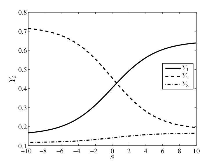
The interfacial tension of the $\alpha\beta$-interface in the far-field limit is given by

References

- [1] C.-Y. Lin, M. Widom, and R. F. Sekerka, Physical Review E 85, 011120 (2012)
- [2] J. W. Gibbs, The Collected Works of J. Willard Gibbs: Thermodynamics, Vol. 1 (Longmans, Green, 1928)
- [3] J. S. Rowlinson and B. Widom, Molecular theory of capillarity (Dover, 2002)
- [4] F. E. Neumann, “Vorlesungen über die theorie der capillarität (ed. a. wangerin),” (Teubner, Leipzig, 1894) Chap. 6 §1, pp. 161–2
- [5] A. W. Adamson and A. P. Gast, Physical chemistry of surfaces (Wiley-Interscience, 1997)
- [6] J. Gaydos and A. W. Neumann, Journal of colloid and interface science 120, 76 (1987)
- [7] J. Drelich, J. D. Miller, and J. Hupka, Journal of colloid and interface science 155, 379 (1993)
- [8] M. Grunze, Science 283, 41 (1999)
- [9] B. H. Weigl and P. Yager, Science 283, 346 (1999)
- [10] A. I. Hienola, P. M. Winkler, P. E. Wagner, H. Vehkamäki, A. Lauri, I. Napari, and M. Kulmala, The Journal of chemical physics 126, 094705 (2007)
- [11] E. Sackmann and R. F. Bruinsma, ChemPhysChem 3, 262 (2002)
- [12] J. Fukai, Y. Shiiba, T. Yamamoto, O. Miyatake, D. Poulikakos, C. M. Megaridis, and Z. Zhao, Physics of Fluids 7, 236 (1995)
- [13] D. Bonn, J. Eggers, J. Indekeu, J. Meunier, and E. Rolley, Reviews of modern physics 81, 739 (2009)
- [14] J. O. Indekeu, Physica A: Statistical Mechanics and its Applications 389, 4332 (2010)
- [15] A. Amirfazli and A. W. Neumann, Advances in colloid and interface science 110, 121 (2004)
- [16] L. Schimmele, M. Napiórkowski, and S. Dietrich, The Journal of chemical physics 127, 164715 (2007)
- [17] D. M. Anderson, G. B. McFadden, and A. A. Wheeler, Annual review of fluid mechanics 30, 139 (1998)
- [18] L. D. Landau and E. M. Lifshitz, Phys. Zeit. Sowjetunion 8 (1935), see also, ”Electrodynamics of Continuous Media”,§45, p.158, reprinted by Beijing World Publishing Cooperation by arrangement with Butterworth-Heinemann (1999)
- [19] A. Umantsev, Field Theoretic Method in Phase Transformations, Vol. 840 (Springer New York, 2012)
- [20] I. Szleifer and B. Widom, Mol. Phys. 75, 925 (1992)
- [21] K. Koga, J. O. Indekeu, and B. Widom, Faraday Discuss. 146, 217 (2010)
- [22] K. Koga and B. Widom, J. Chem. Phys. 128, 114716 (2008)
- [23] K. Koga, J. O. Indekeu, and B. Widom, Physical review letters 104, 36101 (2010)
- [24] C. Lin, Mean-field density functional theory of a three-phase contact line (PhD thesis, Carnegie Mellon University, 2012)
- [25] C. Varea and A. Robledo, Physica A: Statistical and Theoretical Physics 183, 12 (1992)
- [26] J. Kerins and M. Boiteux, Physica A 117, 575 (1983)