Numerical Investigation of Nonisothermal Reversed Stagnation-point Flow

Several application of such have also appeared in the recent literature, for example, in some simplified cases a fluid travels through a rigid body (e.g., missile, sports ball, automobile, spaceflight vehicle), or in oil recovery industry crude oil that can be extracted from an oil field is achieved by hot water injection, as shown in Fig. (1.1), or equivalently, an external flow impinges on a stationary point called stagnation-point that is on the surface of a submerged body in a flow, of which the velocity at the surface of the submerged object is zero. Moreover, the streamline is perpendicular to the surface of the rigid body. The study of the flow motion at stagnation point is of importance in oil recovery industry that develops techniques to efficiently recover oil, gas, and other minerals while reducing environmental impacts using various pollution remediation and greenhouse gas reduction techniques.

The classic problems of two-dimensional stagnation-point flows can be analyzed exactly by Hiemenz [5]. The result is an exact solution for flow directed perpendicular to an infinite flat plate. Howarth [6] and Davey [7] extended the two-dimensional and axisymmetric flows to three dimensions, and Wang [8] studied the case for obliquely-impacting jets. The similarity solutions for the temperature field were studied by Eckert [9]. Case corresponding a step change in wall temperature or in wall heat flux in laminar steady flows at a stagnation point has been also investigated by several authors (see Chao et al. [10], Sano [11] and Gorla [12]). Further, Lok et al. [13] investigated the mixed convection near non-orthogonal stagnation point flow on a vertical plate with uniform surface heat flux, where the results published are very good with present value of the normalized temperature at the wall for the constant wall temperature boundary condition.

On the contrary, when the external flow is extracted away from the stagnation-point shown in Fig. (1.1), the flow in the vicinity of this ”reversed stagnation point” is governed by boundary-layer separation and vorticity generation and the reversed stagnation-point flow develops. Reversed stagnation-point flow is a flow in which the component of velocity normal to a wall is outward the wall everywhere in the region concerned. Reversed stagnation-point flows against an infinite flat wall do not have analytic solution in two dimensions, but certain reverse flows have solution in three dimensions [7].

Proudman and Johnson [1] first suggested that the convection terms dominate in considering the inviscid equation in the body of the fluid. By introducing a very simple function of a particular similarity variable and neglecting the viscous forces in their analytic result for region sufficient far from the wall, they obtained an asymptotic solution in reversed stagnation-point flow, describing the development of the region of separated flow for large time $t$. In their solution, the phenomenon of separation is described near a plane that represents the rear-stagnation point of a cylinder is set in motion impulsively with a constant velocity normal to the surface of the plane. Robins and Howarth [14] have recently extended the asymptotic solution, finding higher order terms by singular perturbation methods. They indicated that the viscous forces cannot be ignored in the governing equation because of a consistent asymptotic expansion in both this outer inviscid region and also in the inner region near the plane. Smith [15] generalized the solution of Proudman and Johnson with both viscous and convection terms in balance by considering the monotonic potential flow when the time is relatively large. Shapiro [16] obtained a solution for unsteady reversed stagnation-point flow with injection or suction. These unsteady flows fit within a class of similarity transformations originally identified by Birkhoff using a group-theoretic approach.

This thesis focuses on the challenging problem of numerical modeling for a nonisothermal reversed stagnation-point flow. The primary objective of the present study is to determine the main characteristics of the flow at reversed stagnation-point. This includes the flow profile, the separation zone, the dividing streamline and the nonisothermal temperature profile. The other objective is to briefly verify the simulation data for the reversed stagnation point.

Chapter 2 is dedicated to developing the governing equation of flow and heat transfer modeling used in this research. Chapter 3 investigates the nature of the development of two-dimensional laminar flow of an incompressible fluid near the reversed stagnation-point. Similarity solutions of two-dimensional reversed stagnation-point flow are investigated by simplifying the full Navier-Stokes equations coupled to the energy equation, describing the motion of nonisothermal fluid substances. The model is valid if the fluid velocity is small compared with the speed of sound and the fluid is treated as Newtonian. Chapter 4 describes the implementation of the algorithm used to achieve the objectives outlined above. Specific information is provided about the individual solvers and details of the interface of simulation. Details of the mesh generation and the efficacy of the CFD solver are provided. Chapter 5 focuses on numerical simulations on the reversed stagnation-point flow. This chapter provides result and discussion of the model provided. The final chapter summarizes and provides conclusions of the research, and recommends future work.

In an incompressible fluid, the density of an element of fluid is not affected by any changes in pressure. If the relative speeds within a flow are low enough (typically Mach number less than $0.3$), thermodynamic effects and density changes due to changes in pressure become negligible. If density is constant and mass is conserved so is volume. This condition is called the equation of continuity and expressed mathematically as the divergence of flow velocity $\boldsymbol{\vec{V}}$ is zero

$$\nabla\cdot\boldsymbol{\vec{V}}=0$$

(2.1)

Essentially what goes into a differential volume must exit it simultaneously. Coupling this equation with conservation of momentum makes the system fully determined, without need of the energy equation or an equation of state, and yields extremely efficient simulations. The flows and solution methods can be greatly different; however, they all start with the same underlying defined as the differential element of the continuous Navier-Stokes equations.

Models for Newtonian fluids undergoing incompressible flow make use of the approximation that dynamic viscosity $\mu$ is a constant. Performing a force balance and making use of the continuity equation leads to the Navier-Stokes equations [17]:

$$\rho\frac{D\boldsymbol{\vec{V}}}{Dt}=-\nabla p+\mu\nabla^{2}\boldsymbol{\vec{V}}+\boldsymbol{\vec{f}}$$

(2.2)

${D\boldsymbol{\vec{V}}}/{Dt}$ is the material derivative of flow velocity

$$\frac{D\boldsymbol{\vec{V}}}{Dt}=\frac{\partial\boldsymbol{\vec{V}}}{\partial t}+(\boldsymbol{\vec{V}}\cdot\nabla)\boldsymbol{\vec{V}}$$

(2.3)

representing the convective acceleration in the fluid motion. The physical principle of momentum transfer is Newton’s second law. Equation (2.2) is just Newton’s second law $\boldsymbol{\vec{F}}=m\boldsymbol{\vec{a}}$ for a fluid element subject to the external force $\boldsymbol{\vec{f}}$ and to the forces arising from pressure gradient $-\nabla p$ and viscosity $\mu\nabla^{2}\boldsymbol{\vec{V}}$.

We begin with writing the governing equation in conservative velocity form in the Cartesian coordinates [18] and neglecting the external force $\boldsymbol{\vec{f}}$:

	$$\displaystyle\frac{\partial u}{\partial x}+\frac{\partial v}{\partial y}=0$$		(2.4a)
	$$\displaystyle\frac{\partial u}{\partial t}+u\frac{\partial u}{\partial x}+v\frac{\partial u}{\partial y}=-\frac{1}{\rho}\frac{\partial p}{\partial x}+\nu\left(\frac{\partial^{2}u}{\partial x^{2}}+\frac{\partial^{2}u}{\partial y^{2}}\right)$$		(2.4b)
	$$\displaystyle\frac{\partial v}{\partial t}+u\frac{\partial v}{\partial x}+v\frac{\partial v}{\partial y}=-\frac{1}{\rho}\frac{\partial p}{\partial y}+\nu\left(\frac{\partial^{2}v}{\partial x^{2}}+\frac{\partial^{2}v}{\partial y^{2}}\right)$$		(2.4c)

Here $u$ and $v$ are the components of flow velocity $\boldsymbol{\vec{V}}(u,v)$, $\rho$ is the fluid density, $p$ is the fluid pressure, $\nu=\mu/\rho$ is the kinematic viscosity. The viscous fluid flows in a rectangular Cartesian coordinates $(x,y,z)$, Fig. 2.1, illustrates the motion of external flow directly moving perpendicular out of an infinite flat plane wall. The origin is the so-called stagnation point and $z$ is the normal to the plane.

What we are concerned about is the two-dimensional reversed stagnation-point flow in unsteady state. The total fluid domain is bounded by an infinite plane $y=0$, the fluid remains at rest when time $t<0$. At $t=0$, it starts impulsively in motion which is determined by the stream function

$$\psi=-\alpha xy$$

(2.5)

where $\alpha$ is a positive rate of strain [18]. At large distances far above the planar boundary, the existence of the potential flow implies an inviscid boundary condition. Far away from the wall the flow is of a constant $V_{0}$ along the $y$-axis. Because of the axisymmetric configuration, the flow field is considered in right-hand side region only. For such a flow the components of velocity are easily given from the relationships

	$$\displaystyle u=-\alpha x$$		(2.6a)
	$$\displaystyle v=V_{0}$$		(2.6b)

Here $\alpha$ is a constant proportional to $V_{0}/L$, $V_{0}$ is the external flow velocity removing from the plane and $L$ is the characteristic length. We have $u=0$ at $x=0$ and $v=0$ at $y=0$, but the no-slip boundary at wall $(y=0)$ cannot be satisfied.

The equation of continuity (2.4a) is integrated by introducing the stream function $\psi$:

$$u=\displaystyle\frac{\partial\psi}{\partial y}\qquad\mathrm{and}\qquad v=\displaystyle-\frac{\partial\psi}{\partial x}$$

(2.7)

For reversed stagnation flow without friction (ideal fluid flow), the stream function may be written as

$$\psi=\psi_{i}=-A_{i}xy$$

(2.8)

where $A_{i}$ is a constant and from which

$$u_{i}=-A_{i}x\qquad\mathrm{and}\qquad v_{i}=A_{i}y.$$

(2.9)

We have $u_{i}=0$ at $x=0$ and $v_{i}=0$ at $y=0$, but the no-slip boundary at wall $(y=0)$ cannot be satisfied.

Since for a (real) viscous fluid the flow motion is determined by only two factors, the kinematic viscosity $\nu$ and $\alpha$, consistent with the initial and boundary conditions that $\psi$ is proportional to $x$ for all value of $y$ and $t$. Provided that the surface is an infinite plane wall, a following modified stream function is introduced, see Proudman and Johnson [1]:

	$$\displaystyle\psi=-\sqrt{A\nu}xf(\eta,\tau)$$		(2.10a)
	$$\displaystyle\eta=\sqrt{\frac{A}{\nu}}y$$		(2.10b)
	$$\displaystyle\tau=At$$		(2.10c)

where $\eta$ is the non-dimensional distance from wall and $\tau$ is the non-dimensional time. Noting that the stream function automatically satisfies equation of continuity (2.4a). Substituting $u$ and $v$ into the governing equations results a simplified partial differential equation. From the definition of the stream function, we have

	$$\displaystyle u=\frac{\partial\psi}{\partial y}=-Axf_{\eta}$$		(2.11a)
	$$\displaystyle v=-\frac{\partial\psi}{\partial x}=\sqrt{A\nu}f$$		(2.11b)

Note that $A$ has the dimension as ”1/time”. The governing equations can be simplified by a similarity transformation when several independent variables appear in specific combinations, in flow geometries involving infinite or semi-infinite surfaces. By introducing coordinate variable transformation, the number of independent variables is reduced by one or more. The original system of partial differential equations can be simplified into the following pair of partial differential equations

	$$\displaystyle-A^{2}xf_{\eta\tau}+A^{2}x(f_{\eta})^{2}-A^{2}xff_{\eta\eta}=-\frac{1}{\rho}\frac{\partial p}{\partial x}-A^{2}xf_{\eta\eta\eta}$$		(2.12a)
	$$\displaystyle A\sqrt{A\nu}f_{\tau}+A\sqrt{A\nu}ff_{\eta}=-\frac{1}{\rho}\frac{\partial p}{\partial y}+A\sqrt{A\nu}f_{\eta\eta}$$		(2.12b)

The pressure gradient can be again reduced by a further differentiation equation (2.12b) with respect to $x$. That is

$$\frac{\partial^{2}p}{\partial x\partial y}=0$$

(2.13)

and equation (2.12a) reduces to

$$[f_{\eta\tau}-(f_{\eta})^{2}+ff_{\eta\eta}-f_{\eta\eta\eta}]_{\eta}=0.$$

(2.14)

or the equation becomes a differential equation for $f$ [19]

$$f_{\eta\tau}-(f_{\eta})^{2}+ff_{\eta\eta}-f_{\eta\eta\eta}=\mathrm{function~of~}\tau\mathrm{~only}.$$

(2.15)

The initial and boundary conditions are

	$$\displaystyle f(\eta,0)\equiv\eta~~~~~~~~~~~~~~~(\eta\neq 0)$$		(2.16a)
	$$\displaystyle f(0,\tau)=f_{\eta}(0,\tau)=0~~(t\neq 0)$$		(2.16b)
	$$\displaystyle f(\infty,\tau)\sim\eta~~~~~~~~~~~~~~~~~~~~~~$$		(2.16c)

These follow from the impermeability condition of the wall (from $v(x,0,\tau)=0$ it follows that $f(0,\tau)=0$) and from the no-slip condition (from $u(x,0,\tau)=0$ it follows that $f_{\eta}(0,\tau)=0$).

Proudman and Johnson suggested that at large distances from the wall ($\eta\rightarrow\infty$) the velocity $v(x,\eta,\tau)$ should pass over smoothly into that for inviscid $V_{0}$. Here they have employed $f_{\eta\eta}(\infty)=f_{\eta\eta\eta}(\infty)=0,$ which implies that the flow matches smoothly with the inviscid flow as $\eta\rightarrow\infty$. This leads to the condition $f(\infty,\tau)\sim\eta,$ and thus, the last condition reduces the differential equation (2.14) for $f$ [19]

$$f_{\eta\tau}-(f_{\eta})^{2}+ff_{\eta\eta}-f_{\eta\eta\eta}=-1,$$

(2.17)

with the boundary conditions

	$$\displaystyle f(0,\tau)=f_{\eta}(0,\tau)=0$$		(2.18a)
	$$\displaystyle f_{\eta}(\infty,\tau)=1.~~~~~~~~~~$$		(2.18b)

Here $f_{\eta\eta\eta}$ is proportional to the viscous stress, $f_{\eta\eta}$ is proportional to the shear stress, $f_{\eta}$ is proportional to the x-component of velocity in boundary layer and $f$ is s proportional to the stream function.

It should be noted that the dimensionless velocity distribution $f_{\eta}$ is, from (2.11), independent of the length $x$, and thus equation (2.17) is a similarity equation of the full Navier-Stokes equations at two-dimension reversed stagnation-point. The coordinates $x$ and $y$ are replaced by a dimensionless variable $\eta$. Under the boundary conditions $f_{\eta}(\infty,\tau)=1$, when the flow is in steady state such that $f_{\eta\tau}\equiv 0$, the differential equation has no solution.

In this section our considerations of reversed stagnation-point flow until now have referred only to velocity field. Now we shall extend to include the temperature field in the nonisothermal flow which is at a temperature $T$ different from that of the wall $T_{w}$. It will be assumed that heat energy is transferred to the flow through the wall. Once the velocities are known from the flow analysis, the temperature distributions can be determined by solving the energy equation in the reversed stagnation-point flow.

To include the temperature $T$ in our analysis we must now turn to the thermodynamic properties of fluids. The principle of conservation of energy yields the thermal energy equation [20] for constant-property fluid:

$$\rho c_{p}\left(\frac{\partial T}{\partial t}+u\frac{\partial T}{\partial x}+v\frac{\partial T}{\partial y}\right)=k\left(\frac{\partial^{2}T}{\partial x^{2}}+\frac{\partial^{2}T}{\partial y^{2}}\right)+\mu\Phi$$

(2.19)

where $k$ is the thermal conductivity, $c_{p}$ is the heat capacity, and $\Phi$ is defined as

$$\Phi=2\left[\left(\frac{\partial u}{\partial x}\right)^{2}+\left(\frac{\partial v}{\partial y}\right)^{2}\right]+\left(\frac{\partial u}{\partial y}+\frac{\partial v}{\partial x}\right)^{2}-\frac{2}{3}\left(\frac{\partial u}{\partial x}+\frac{\partial v}{\partial y}\right)^{2}$$

(2.20)

and is called the viscous dissipation since it represents the irreversible conservation of mechanical forms of energy to a thermal form.

If both velocity field and temperature field exist, there is generally also a coupling between these two fields. Since the velocity components $u$ and $v$ appear in the energy equation, a simplification of the energy equation requires to know the actual value of the velocity components. This velocity field would be identical to the velocity components in the reversed stagnation-point flow

	$$\displaystyle u=-Axf_{\eta}$$		(2.21a)
	$$\displaystyle v=\sqrt{A\nu}f$$		(2.21b)

To transform equation (2.19) into a nondimensional form, it is convenient to work with a dimensionless temperature $\theta$ [18]:

$$\theta(\eta,\tau)=\frac{T-T_{w}}{T_{\infty}-T_{w}}$$

(2.22)

where $T_{w}$ and $T_{\infty}$ are the wall temperature and ambient temperature. Considering the case that both $T_{w}$ and $T_{\infty}$ are constant, the required boundary conditions are

$$T(0,t)=T_{w},\qquad T(\infty,t)=T_{\infty}.$$

(2.23)

The fluid temperature $T$ can be treated as a function of $\eta$ and $\tau$ only. Under the assumption that the viscous dissipation is negligible compared to conduction at the wall, we may write the energy equation in the form

$$\theta_{\eta\eta}-\frac{\rho c_{p}\nu}{k}f\theta_{\eta}=\frac{\rho c_{p}\nu}{k}\theta_{\tau}$$

(2.24)

subject to the boundary conditions

$$\theta(0,\tau)=0\qquad\theta(\infty,\tau)=1$$

(2.25)

Equation (2.24) is a second-order partial differential equation with variable coefficient $f(\eta,\tau)$ and the Prandtl number $Pr=\rho c_{p}\nu/k$ is assumed to be constant. Consider the fluid of which $Pr=1$, the thermal boundary layer and the velocity boundary layer collapse, and thus, substituting $\theta=f^{\prime}$, equation (2.17) and (2.24) represent the same equation. It is noticed that in these nonisothermal flows the velocity field is decoupled from the temperature field if the kinematic viscosity $\nu$ is constant and is assumed to be independent of the temperature and pressure. This assumption is valid when the temperature and pressure differences are small within the boundary layer.

Proudman and Johnson [1] first thought over the early stages of the diffusion of the initial vortex sheet at $y=0$. The idea was to divide the flow into two regions: an outer flow region that is inviscid and can sometimes be approximated as potential flow, and an inner flow region where the viscous forces are of the same order as the inertial forces. The general feature of the predicted streamline pattern is sketched in Fig. (3.1).

Proudman and Johnson suggested that, when the flow is near the wall region, the viscous forces are dominant, and the viscous term in the governing Navier-Stokes equations is important only near the boundary. On the contrary, the viscous forces were neglected far away from the wall. The convection terms dominate the motion of external flow in considering the inviscid equation in the fluid. Ignoring the viscous stress in equation (2.17) yields an inviscid equation

$$f_{\eta\tau}-(f_{\eta})^{2}+ff_{\eta\eta}+1=0.$$

(3.1)

They contemplated the similarity of the inviscid equation in the form

$$f(\eta,\tau)=\lambda({\tau})F(\gamma),~~~\gamma=\eta/\lambda({\tau})$$

(3.2)

Substituting equation (3.2) in (3.1) results in

$$\frac{\dot{\lambda}}{\lambda}\gamma F^{\prime\prime}-F^{\prime 2}+FF^{\prime\prime}=-1,$$

(3.3)

so that

$$\frac{\dot{\lambda}}{\lambda}=\mathrm{constant}=k,~~\mathrm{or~~}\lambda=e^{k\tau}$$

(3.4)

A solution to this equation that satisfies $F=1$ with exponential error as $\eta\rightarrow\infty$ is only possible when $k=1$; Proudman and Johnson finally obtained an asymptotic similarity solution of

$$f(\eta,\tau)={\eta}-\frac{2e^{\tau}}{c}(1-e^{-c{\eta}e^{-\tau}})$$

(3.5)

where $c$ is a constant of integration, representing the uncertainty in the precise position of the time origin. In the asymptotic solution (3.5), the constant $c$ always appears multiplying the similarity variable, i.e. $c\eta e^{-\tau}$. A change from $\tau$ to $\tau+\Delta\tau$ can be included in the constant $c$. The improved numerical evaluations of Robins and Howarth [14] estimated the value of $c$ to be $3.51$. This solution describes an exponential decay of vorticity in the outer region, moving away from the plane with a constant velocity.

The viscous layer develops as a consequence of the no-slip boundary condition at the wall. In the inner region the viscous term cannot be neglected and a further solution must be found which satisfies the no-slip condition on the wall. When $\tau\rightarrow\infty$, the solution (3.5) yields the steady flow

$$f\sim-\eta~~~~\mathrm{and}~~~~~f^{\prime}\sim-1$$

(3.6)

which becomes the outer boundary condition for the viscous flow near the boundary. Substituting in equation (2.17) yields

	$$\displaystyle f^{\prime\prime\prime}-ff^{\prime\prime}+(f^{\prime})^{2}-1=0$$		(3.7a)
	$$\displaystyle f(0)=f^{\prime}(0)=0~~~~~~~~~~~~~$$		(3.7b)
	$$\displaystyle f^{\prime}(\infty)=-1~~~~~~~~~~~~~~~~~~~$$		(3.7c)

This is exactly the classic stagnation-point problem (Hiemenz [5]) by changing the sign in $f$. It is a third-order nonlinear ordinary differential equation and does not have an analytic solution, and thus it is necessary to solve it numerically. The numerical solution of classic stagnation-point problem is shown in Figure (3.2).

Although an asymptotic solution was obtained, it can easily been observed that this is not valid when the viscous term $f_{\eta\eta\eta}$ is neglected within the total flow field. Robins and Howarth [14] studied higher order terms by singular perturbation methods and indicated that a consistent asymptotic expansion occurs in both outer inviscid region and also in the inner region that must exist close to the wall where the viscous forces need to be included. It is not quite appropriate to say Proudman and Johnson are wrong because of neglecting the viscous term in their analytic result for region sufficient far from the wall, but in such a case neglecting the viscous terms within the total flow field can be improved. The next section will discuss the nonexistence of the exact solutions with the boundary condition $f_{\eta}(\infty,\tau)=1$ for steady case.

In this section, a mathematical proof indicates that all of the steady solutions, however, do not satisfy the boundary condition $f_{\eta}(\infty,\tau)=1$.

When $f_{\eta\tau}\equiv 0$, Eq. (2.17) reduces to

	$$\displaystyle f^{\prime\prime\prime}-ff^{\prime\prime}+(f^{\prime})^{2}-1=0$$		(3.8a)
	$$\displaystyle f(0)=f^{\prime}(0)=0~~~~~~~~~~~~~$$		(3.8b)
	$$\displaystyle f^{\prime}(\infty)=1~~~~~~~~~~~~~~~~~~~~~$$		(3.8c)

where the prime denotes the derivative with respect to $\eta$.

Proof. Rearrange equation (3.8) yields

$$f^{\prime\prime\prime}=1-(f^{\prime})^{2}+ff^{\prime\prime}$$

(3.9)

Suppose for $\eta=\eta_{0}$, we have $f^{\prime}(\eta_{0})=1$ and $f^{\prime\prime}(\eta_{0})=0$. Afterwards, it follows from the derivatives of equation (3.9) that $f^{\prime\prime\prime}$ and all higher derivatives are zero when $\eta=\eta_{0}$. Consider a variable transformation

	$$\displaystyle\varpi(\eta)=f^{\prime}(\eta)$$
	$$\displaystyle\varpi(\eta_{0})=1$$		(3.10)

Expand the function into Taylor’s series near $\eta_{0}$, we have

	$\displaystyle f^{\prime}(\eta)=\varpi(\eta)$	$\displaystyle=$	$\displaystyle\sum_{n=0}^{\infty}\frac{\varpi^{(n)}(\eta_{0})}{n!}(\eta-\eta_{0})^{n}$
		$\displaystyle=$	$\displaystyle\varpi(\eta_{0})+\sum_{n=1}^{\infty}\frac{\varpi^{(n)}(\eta_{0})}{n!}(\eta-\eta_{0})^{n}$
		$\displaystyle=$	$\displaystyle 1+\sum_{n=1}^{\infty}\frac{\varpi^{(n)}(\eta_{0})}{n!}(\eta-\eta_{0})^{n}$
		$\displaystyle\equiv$	$\displaystyle 1$

Hence, the boundary condition $f^{\prime}(0)=0$ is thus not satisfied and the Lemma is proved.

Proof: From equation (3.9), when $f^{\prime}$ has a stationary value, it means $f^{\prime\prime}=0$ and equation (3.9) becomes

$$f^{\prime\prime\prime}=1-(f^{\prime})^{2}$$

(3.11)

If $|f^{\prime}|<1$, $f^{\prime\prime\prime}>0$ and it is minima. Else if $|f^{\prime}|>1$, $f^{\prime\prime\prime}<0$ and it is maxima. Eventually, the lemma is proved.

Proof: Consider a region where $(\eta_{1},\eta_{2})$ is far away from the origin. Multiply $f^{\prime\prime}$ to equation (3.9) and integrate it between $\eta_{1}$ and $\eta_{2}$ with respect to $\eta$.

$$f^{\prime\prime}f^{\prime\prime\prime}=f^{\prime\prime}-(f^{\prime})^{2}f^{\prime\prime}+f(f^{\prime\prime})^{2}$$

$$\int_{\eta_{1}}^{\eta_{2}}f^{\prime\prime}f^{\prime\prime\prime}d\eta=\int_{\eta_{1}}^{\eta_{2}}[f^{\prime\prime}-(f^{\prime})^{2}f^{\prime\prime}+f(f^{\prime\prime})^{2}]d\eta$$

$$\displaystyle\frac{1}{2}[(f^{\prime\prime})^{2}]_{\eta_{1}}^{\eta_{2}}=[f^{\prime}-\frac{1}{3}(f^{\prime})^{3}]_{\eta_{1}}^{\eta_{2}}+\int_{\eta_{1}}^{\eta_{2}}f(f^{\prime\prime})^{2}d\eta$$

When $f^{\prime}(\infty)\to 1$, it is required that $f^{\prime\prime}(\eta_{1})=f^{\prime\prime}(\eta_{2})=0$ and thus

$$[f^{\prime}-\frac{1}{3}(f^{\prime})^{3}]_{\eta_{1}}^{\eta_{2}}=-L$$

whereas $\displaystyle L=\int_{\eta_{1}}^{\eta_{2}}f(f^{\prime\prime})^{2}d\eta$ is always positive and we can obtain

$$[f^{\prime}-\frac{1}{3}(f^{\prime})^{3}]_{\eta_{1}}^{\eta_{2}}<0$$

$$f^{\prime}(\eta_{2})-\frac{1}{3}[f^{\prime}(\eta_{2})]^{3}<f^{\prime}(\eta_{1})-\frac{1}{3}[f^{\prime}(\eta_{1})]^{3}$$

$$[f^{\prime}(\eta_{2})]^{3}-3f^{\prime}(\eta_{2})>[f^{\prime}(\eta_{1})]^{3}-3f^{\prime}(\eta_{1})$$

Consider $G=f^{\prime 3}-3f^{\prime}$ as a function of $f^{\prime}$, then

$$G^{\prime}=3f^{\prime 2}-3$$

As $f^{\prime}=1$, then $G^{\prime}(1)=0$, which makes G a minimum. We do not have $f^{\prime}(\eta_{i})=1$ as $\eta_{i}\to\infty$

Proof : When $|f^{\prime}|<1$, since $f^{\prime}\to 1$ as $\eta\to\infty$, then $f^{\prime\prime}$ must be greater than zero. Hence, recall from equation (3.9),

$$f^{\prime\prime\prime}=1-(f^{\prime})^{2}+ff^{\prime\prime}>0.$$

for all $\eta>\eta_{0}$. After integrating $f^{\prime\prime\prime}(\eta)>0$ from $\eta_{0}$ to $\eta>\eta_{0}$, we have

$$f^{\prime\prime}(\eta)>f^{\prime\prime}(\eta_{0})=K>0.$$

Another integration from $\eta_{0}$ to $\eta>\eta_{0}$ yields

$$f^{\prime}(\eta)>f^{\prime}(\eta_{0})+K(\eta-\eta_{0}).$$

By Lemma $2$, $f^{\prime}(\eta)$ has at most one stationary value because one cannot have two consecutive stationary values which are both minima. Since $f^{\prime\prime}(\eta)>0$, when $\eta\to\infty$, $f^{\prime}(\eta)\to\infty.$ It violates that $f^{\prime}(\eta)\to 1$. A similar argument shows that a solution cannot approach to 1 when $|f^{\prime}|>1$.

The remaining option is that $f(\eta)$ oscillates about 1 as $f^{\prime}(\infty)\to 1$. But this would imply an infinite number of changes in concavity of $f^{\prime}$ as $\eta\to\infty$. Once $f^{\prime}(\eta)$ vibrates from concave upward $(f^{\prime\prime\prime}>0)$ to concave downward $(f^{\prime\prime\prime}<0)$, as $f(\eta)$ becomes great enough, it cannot turn concave upward again [21]. It requires a point $\eta_{1}$ such that

$$f^{(4)}(\eta_{1})=0$$

and

$$f^{(5)}(\eta_{1})\geq 0$$

Differentiating equation (3.9) gives

$$f^{(4)}=ff^{\prime\prime\prime}-f^{\prime}f^{\prime\prime}$$

(3.12)

and

$$f^{(5)}=ff^{(4)}-(f^{\prime\prime})^{2}$$

(3.13)

Evaluating these at $\eta_{1}$ yields

$$f^{(5)}(\eta_{1})=-[f^{\prime\prime}(\eta_{1})]^{2}\leq 0$$

If $f^{\prime\prime}(\eta_{1})\neq 0$ we get an immediate contradiction. On the other hand, if $f^{\prime\prime}(\eta_{1})=0$, equation (3.12) implies that $f^{\prime\prime\prime}=0$. But from equation (3.9) we see that $f^{\prime\prime}(\eta_{1})=f^{\prime\prime\prime}(\eta_{1})=0$ implies the desired contradiction that

$$f^{\prime}(\eta)\equiv 1.$$

Thus, since $f^{\prime}(\eta)$ cannot ultimately approach to 1 from above or below, nor in an oscillatory manner, no solution to equation (3.8) exists. Reversed stagnation-point flow against an impermeable flat wall does not exist in two-dimensional steady case.

Similarity solutions of reversed stagnation-point flow with different boundary conditions have been published in [22, 23, 24]. Numerical simulation of reversed stagnation-point flow with full Navier-Stokes equations has been studied in [25]. According to the previous work, the governing equations in reversed stagnation-point flow are

$$f_{\eta\tau}-(f_{\eta})^{2}+ff_{\eta\eta}-f_{\eta\eta\eta}+1=0,$$

(2.17)

$$\theta_{\eta\eta}-{Pr}~f\theta_{\eta}={Pr}~\theta_{\tau}$$

(2.24)

The above equations subject to the boundary conditions (2.17) and (2.24) are nonlinear third-order partial differential equations. They do not admit similarity solution and numerical or perturbation methods are required to solve the problem.

We shall, however, use here a numerical method. It is an implicit finite-difference method with second-order accuracy. The partial differential equations can be expressed as approximate expressions, so that it is easy to program the solution of large numbers of coupled equation.

We start with rewriting the partial differential equations in the form:

	$$\displaystyle f_{\eta\tau}=f_{\eta\eta\eta}+(f_{\eta})^{2}-1+ff_{\eta\eta}$$		(3.14a)
	$$\displaystyle\theta_{\tau}=\frac{1}{Pr}\theta_{\eta\eta}-f\theta_{\eta}$$		(3.14b)

and introducing the new dependent variables

	$$\displaystyle h=1-f_{\eta}$$		(3.15a)
	$$\displaystyle g=\theta$$		(3.15b)

The equations can be rewritten as

	$$\displaystyle h_{\tau}=h_{\eta\eta}+2h-h^{2}+h_{\eta}\int(1-h)~d\eta$$		(3.16a)
	$$\displaystyle g_{\tau}=\frac{1}{Pr}g_{\eta\eta}-g_{\eta}\int(1-h)~d\eta$$		(3.16b)

We now contemplate the net rectangle in the $\tau-\eta$ plane shown in Fig. (3.3) and the net points defined as below:

$$\eta^{0}=0,~~~~~~\eta_{j}=\eta_{j-1}+\Delta\eta,~~~j=1,2,...J,~\eta_{J}=\eta_{\infty}$$

$$\tau^{0}=0,~~~~~~\tau^{n}=\tau^{n-1}++\Delta\tau,~~n=1,2,...J,~~~~~~~~~~~$$

Here $n$ and $j$ are just the sequence of numbers that indicate the coordinate location, not tensor indices or exponents.

The partial differential equations are easily discretized by central difference representations with second-order accuracy, for example the finite difference forms for any points are

$$h_{\eta}=\frac{h^{n}_{i+1}-h^{n}_{i-1}}{2\Delta\eta}$$

(3.17)

and

$$h_{\eta\eta}=\frac{h^{n}_{i+1}-2h^{n}_{i}+h^{n}_{i-1}}{\Delta\eta}$$

(3.18)

When $i=0$, since the value of $h^{n}_{i-1}$ is not logical, the derivative is replaced by the forward difference with second-order accuracy

$$h_{\eta}=\frac{-h^{n}_{i+2}+4h^{n}_{i+1}-3h^{n}_{i}}{2\Delta\eta}$$

(3.19)

The finite-difference form of the ODE is written at the midpoint $(\tau^{n},~\eta_{j})$, the discretized equation takes the form

	$$\displaystyle\frac{h^{n+1}_{i}-h^{n}_{i}}{\Delta\tau}=\frac{h^{n+1}_{i+1}-2h^{n+1}_{i}+h^{n+1}_{i-1}}{(\Delta\eta)^{2}}+2h^{n}_{i}~~~~~~~~~~~~~~~~~~~~~~~~~~~~~~~~~~~~~~~~~$$
	$$\displaystyle~~~~~~~~~~~~~~~~~~~~~~~~~~~~~~~~~~~-(h^{n}_{i})^{2}-\frac{h^{n}_{i+1}-h^{n}_{i-1}}{2\Delta\eta}\int^{i\Delta\eta}_{0}(1-h)~d\eta$$		(3.20a)
	$$\displaystyle\frac{g^{n+1}_{i}-g^{n}_{i}}{\Delta\tau}=\frac{g^{n+1}_{i+1}-2g^{n+1}_{i}+g^{n+1}_{i-1}}{Pr(\Delta\eta)^{2}}-\frac{g^{n}_{i+1}-g^{n}_{i-1}}{2\Delta\eta}\int^{i\Delta\eta}_{0}(1-h)~d\eta$$		(3.20b)

This procedure yields the following linear tridiagonal system:

	$$\displaystyle-\beta h^{n+1}_{i+1}+(1+2\beta)h^{n+1}_{i}-\beta h^{n+1}_{i-1}=~~~~~~~~~~~~~~~~~~~~~~~~~~~~~~~~~~~~~~~~~~~~~~~~$$
	$$\displaystyle~~~~~~~~~~~~~~~~~~~~~~~~h^{n}_{i}+\Delta\tau\left[2h^{n}_{i}-(h^{n}_{i})^{2}-\frac{h^{n}_{i+1}-h^{n}_{i-1}}{2}\sum^{i}_{0}(1-h^{n}_{i})\right]$$		(3.21a)
	$$\displaystyle-\frac{\beta}{Pr}g^{n+1}_{i+1}+\left(1+\frac{2\beta}{Pr}\right)g^{n+1}_{i}-\frac{\beta}{Pr}g^{n+1}_{i-1}=~~~~~~~~~~~~~~~~~~~~~~~~~~~~~~~~~~~~~~~~~~$$
	$$\displaystyle~~~~~~~~~~~~~~~~~~~~~~~~~~~~~~~~~~~~~~~~~~~~g^{n}_{i}-\Delta\tau~\frac{g^{n}_{i+1}-g^{n}_{i-1}}{2}\sum^{i}_{0}(1-h^{n}_{i})$$		(3.21b)

where $\beta=\Delta\tau/(\Delta\eta)^{2}$.

The initial conditions are the solutions of the following second-order linear parabolic differential equations

	$$\displaystyle h_{\tau}=h_{\eta\eta}$$		(3.22a)
	$$\displaystyle g_{\tau}=\frac{1}{Pr}g_{\eta\eta}$$		(3.22b)

As can be seen from the energy equation (2.24), equations (3.22) are identical to the heat conduction equation for one-dimensional unsteady temperature field, and thus, there are many solutions to these differential equations in [26]. The desired solutions of (3.22) have the form

	$$\displaystyle h=1-\mathrm{erf}\left(\frac{\eta}{2\sqrt{\tau}}\right)$$		(3.23a)
	$$\displaystyle g=\mathrm{erf}\left(\frac{\eta}{2\sqrt{\tau/Pr}}\right)$$		(3.23b)

where the error function $\mathrm{erf}(z)$ is defined as

$$\mathrm{erf}(z)=\frac{2}{\sqrt{\pi}}\int^{z}_{0}\exp(-\xi^{2})~d\xi$$

(3.24)

When $\tau\rightarrow 0,$ the boundary conditions are convenient to write in the form

$$h^{n}_{0}=g^{n}_{0}=0,~~~~~~~h^{0}_{i}=\mathrm{erf}\left(\frac{\eta_{i}}{2\sqrt{\tau}}\right),~~~~~~~g^{0}_{i}=\mathrm{erf}\left(\frac{\eta_{i}}{2\sqrt{\tau/Pr}}\right)$$

(3.25)

Equations (3.21) are defined as being implicit, as more than one unknown appears in the left hand side. They are unconditionally stable, however, set of linear algebraic equations is required to be solved by the tridiagonal matrix algorithm (TDMA), also known as the Thomas algorithm, which is a simplified form of Gaussian elimination that is applied to evaluate tridiagonal systems of equations.

For the stability of the diffusion difference equation, the condition of $\beta\leq\frac{1}{2}$ must be satisfied. The procedure is straightforward, except for the algebra. The resulting algorithm of the finite-difference method is written in MATLAB, a numerical computing environment allowing matrix manipulations and plotting of functions and data. At our level of discretization, however, we are only able to resolve in small time range. The numerical results of (3.21) are presented in Figures (3.4) to (3.6).

From the Proudman-Johnson solution (3.5), we have

$$\log h=-c\eta e^{\tau}+\log 2,$$

(3.26)

so the graph of $\log h$ against $\eta e^{\tau}$ should provide a straight line of gradient $-c$ if the Proudman-Johnson solution holds. In Figure (3.4b), the graph of $\log h$ against $e^{-\tau+3.5}$ is plotted for different values of $\tau$. As can be seen, the parallel straight lines for large values of $\tau$ agrees well for the Proudman-Johnson solution. The value of $c$ calculated from the gradient of the straight line in Figure (3.4b) is $c=3.5$, which agrees to the estimation of Robins and Howarth.

The following pages (Figures. (3.5) to (3.6)) show the numerical solution of temperature distributions with $\mathrm{Pr}$. It is noted that the dimensionless wall temperature gradient $g^{\prime}(0)$ raises with increase of Prandtl number, but the temperature boundary layer thickness decrease with increase of Prandtl number. Prandtl number is the characteristic number for thermal boundary layers and heat transfer in forced convection. It can be explained by the definition of Prandtl number that inversely proportional to the thermal diffusivity $\alpha$. Prandtl number is a ratio of two quantities which characterize the momentum and heat transport of fluid. In heat transfer problems, the Prandtl number controls the relative thickness of the momentum and thermal boundary layers. When $\mathrm{Pr}$ is small, it means that the heat diffuses very quickly compared to the velocity field. This means that for liquid metals the thickness of the thermal boundary layer is much bigger than the velocity boundary layer.

Figure (3.7) shows the pressure distribution along the $x$- and $\eta$-direction at different values of $\tau=3,4$ and $5$. Lines without markers denote results obtained from numerical procedure and dotted lines are from asymptotic solution. Far away from the wall region, the solution agrees remarkably well for smaller values of $\tau$ with the known asymptotic solution, thus confirming the predictions of the analytical solution. On the other hand, discrepancy occurs as a larger value of τ is applied in the numerical simulation. However, in the region near the stagnation point, a large difference is observed from the results obtained by these two methods in the region near the stagnation point. Numerical findings show that pressure profiles obtained from asymptotic solution and numerical simulation are in tremendously good agreement for smaller value of $\tau$. Discrepancy of results in pressure profiles increases for larger value of $\tau$.

The finite volume method (FVM) is a numerical technique that evaluates partial differential equations (PDEs) in the form of algebraic equations. Similar to the finite difference method, values are calculated at discrete places on a meshed geometry. An advantage of the finite volume method is that it is easy to develop to enable unstructured meshes. This feature gives convenience in processing complicated geometries. Once the mesh of the domain is formulated, those governing equations are able to be solved. The method is applied in many computational fluid dynamics packages, for instance, STAR-CD, FLUENT and OpenFOAM.

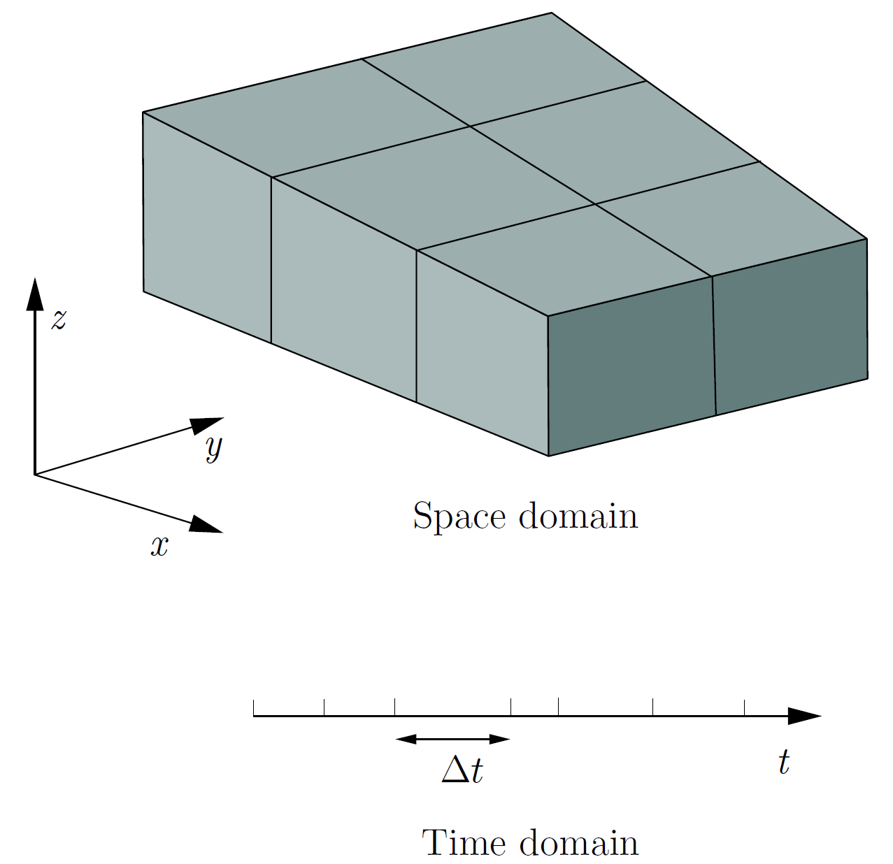
When solving the Navier-Stokes equations, discretization of the solution domain is shown in Figure (4.1). The solution domain consists of a space and a time domain. The space domain is subdivided into a set of very small but finite-sized cells or volumes covering the whole domain. Each cell is stored a set of governing equations to describe the physical phenomenon. Discretization of time involves in subdividing the domain into a set of time steps $\Delta t$, which may alter during a numerical simulation depending on some condition calculated during the simulation.

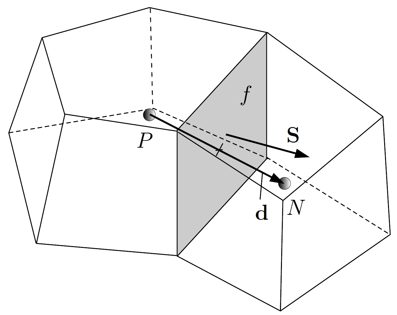
Discretization of space involves in subdividing the domain into a number of cells, or control volumes. A typical cell is shown in Figure (4.2). As can be seen the cells fill the computational domain without overlap. Dependent variables and other properties are principally assigned at the cell centroid, but it is possible to assign them on faces or vertices. The cell is bounded by a set of flat faces, given the generic label.

The purpose of equation discretization is to transform one or more governing equations into a corresponding system of algebraic equations. The solution of this system approximates the solution to the original partial differential equations at certain locations in space and time. As for compressible flows, the mass conservation is a transport equation for density. With an additional energy equation $p$ can be constructed from a thermodynamic relation (ideal gas law).

And for incompressible flows, density variation is not correlated to the pressure field. Mass conservation is a constraint on the velocity field. Combined with the momentum equation, an equation for the pressure can be derived analytically. Consider the continuity and Navier-Stokes equations

$$\nabla\cdot\boldsymbol{\vec{V}}=0$$

(4.1)

$$\frac{\partial}{\partial t}\boldsymbol{\vec{V}}+\nabla\cdot\boldsymbol{\vec{V}}\boldsymbol{\vec{V}}=-\frac{1}{\rho}\nabla p+\nu\nabla^{2}\boldsymbol{\vec{V}}$$

(4.2)

where $\rho$ is the density, $p$ is the pressure, $\nu$ is the kinematic viscosity. The principle of conservation of energy will yield the equation of energy for negligible viscous dissipation:

$$\frac{\partial T}{\partial t}+\nabla\cdot T\boldsymbol{\vec{V}}=\alpha\nabla^{2}T$$

(4.3)

where $\alpha=k/\rho c_{p}$ is thermal diffusivity.

BIBLIOGRAPHY

- [1] I. Proudman and K. Johnson, “Boundary-layer growth near a rear stagnation point,” Journal of Fluid Mechanics, vol. 12, no. 02, pp. 161–168, 1962.
- [2] N. LTD., FOAM Programmer’s Guide. Nabla LTD., 2001.
- [3] W. Lyons and G. Plisga, Standard handbook of petroleum and natural gas engineering. Gulf Professional Publishing, 2005.
- [4] H. Oertel and L. Prandtl, Prandtl’s essentials of fluid mechanics. Springer Verlag, 2004.
- [5] K. Hiemenz, “Die Grenzschicht an einem in den gleichförmigen Flüssigkeitsstrom eingetauchten geraden Kreiszylinder, Dingl. Polytech,” J, vol. 326, pp. 321–410, 1911.
- [6] L. Howarth, “CXLIV. The boundary layer in three dimensional flow.-Part II. The flow near a stagnation point,” Philosophical Magazine (Series 7), vol. 42, no. 335, pp. 1433–1440, 1951.
- [7] A. Davey, “Boundary-layer flow at a saddle point of attachment,” Journal of Fluid Mechanics, vol. 10, pp. 593–610, 1961.
- [8] C. Wang, “The unsteady oblique stagnation point flow,” Physics of Fluids, vol. 28, pp. 2046–2049, 1985.
- [9] E. Eckert, Die Berechnung des Wärmeübergangs in der laminaren Grenzschicht umströmter Körper. VDI-Forschunhsheft, 1942.
- [10] B. Chao and D. Jeng, “Unsteady stagnation point heat transfer,” J. Heat Transfer, vol. 87, pp. 221–230, 1965.
- [11] T. Sano, “Unsteady stagnation point heat transfer with blowing or suction,” Journal of Heat Transfer, vol. 103, p. 448, 1981.
- [12] R. Gorla, “The final approach to steady state in a nonsteady axisymmetric stagnation point heat transfer,” Heat and Mass Transfer, vol. 22, no. 1, pp. 37–44, 1988.
- [13] Y. Lok, N. Amin, and I. Pop, “Mixed convection near a non-orthogonal stagnation point flow on a vertical plate with uniform surface heat flux,” Acta Mechanica, vol. 186, no. 1, pp. 99–112, 2006.
- [14] A. Robins and J. Howarth, “Boundary-layer development at a two-dimensional rear stagnation point,” Journal of Fluid Mechanics, vol. 56, no. 01, pp. 161–171, 1972.
- [15] S. Smith, “The development of the boundary layer at a rear stagnation point,” Journal of Engineering Mathematics, vol. 11, no. 2, pp. 139–144, 1977.
- [16] A. Shapiro, “An analytical solution of the navier-stokes equations for unsteady backward stagnation-point flow with injection or suction,” ZAMM-Journal of Applied Mathematics and Mechanics/Zeitschrift für Angewandte Mathematik und Mechanik, vol. 86, no. 4, pp. 281–290, 2006.
- [17] O. Zikanov, Essential Computational Fluid Dynamics. John Wiley & Sons, 2011.
- [18] F. White, Viscous fluid flow. McGraw-Hill series in mechanical engineering, McGraw-Hill Higher Education, 1991.
- [19] H. Schlichting and K. Gersten, Boundary-Layer Theory. Physics and astronomy online library, Springer, 2000.
- [20] L. C. Burmeister, Convective heat transfer. A Wiley-Interscience publication, Wiley, 1993.
- [21] J. Paullet and P. Weidman, “Nonexistence of solutions for reverse radial stagnation flow with transpiration,” Applied Mathematics Letters, vol. 18, no. 9, pp. 1009–1012, 2005.
- [22] V. Sin and C. Chio, “Reversed stagnation-point flow: Numerical simulation and asymptotic solution,” in System Science and Engineering (ICSSE), 2011 International Conference on, pp. 17–22, IEEE, 2011.
- [23] V. K. Sin and C. K. Chio., “Another Approach of Similarity Solution in Reversed Stagnation-point Flow,” in World Academy of Science, Engineering and Technology, vol. 59, 2011.
- [24] V. K. Sin and C. K. Chio., “Unsteady Reversed Stagnation-Point Flow over a Flat Plate,” International Journal of Computational and Mathematical Sciences, vol. 6, pp. 153–158, 2012.
- [25] V. K. Sin and C. K. Chio, Computation of Non-Isothermal Reversed Stagnation-Point Flow over a Flat Plate, ch. Computational Simulations and Applications, pp. 159–174. InTech, 2011. ISBN: 978-953-307-430-6.
- [26] S. Goldstein and L. Rosenhead, “Boundary layer growth,” in Mathematical Proceedings of the Cambridge Philosophical Society, vol. 32, pp. 392–401, Cambridge Univ Press, 1936.
- [27] J. Wendt and J. Anderson, Computational fluid dynamics: an introduction. Von Karman Institute Book, Springer, 2009.
- [28] J. Ferziger and M. Perić, Computational methods for fluid dynamics. Numerical methods: Research and development, Springer-Verlag, 1996.
- [29] J. Tannehill, D. Anderson, and R. Pletcher, Computational fluid mechanics and heat transfer. Series in computational and physical processes in mechanics and thermal sciences, Taylor & Francis, 1997.
- [30] S. Koranne, Handbook of Open Source Tools. Springer, 2010.
- [31] R. Courant and H. Lewy, On the Partial Difference Equations of Mathematical Physics. BiblioBazaar, 2011.
- [32] H. Blasius, “Grenzschichten in flüssigkeiten mit kleiner reibung,” Z. Math. Phys., vol. 56, pp. 1–57, 1908.
- [33] D. Zwillinger, Handbook of differential equations. Academic Press, 1998.
- [34] L. Shampine, I. Gladwell, and S. Thompson, Solving ODEs with MATLAB. Cambridge Univ Pr, 2003.