Nonparametric Estimation of Means on Hilbert Manifolds and Extrinsic Analysis of Mean Shapes of Contours
Abstract
Motivated by the problem of nonparametric inference in high level digital image analysis, we introduce a general extrinsic approach for data analysis on Hilbert manifolds with a focus on means of probability distributions on such sample spaces. To perform inference on these means, we appeal to the concept of neighborhood hypotheses from functional data analysis and derive a one-sample test. We then consider analysis of shapes of contours lying in the plane. By embedding the corresponding sample space of such shapes, which is a Hilbert manifold, into a space of Hilbert-Schmidt operators, we can define extrinsic mean shapes of planar contours and their sample analogues. We apply the general methods to this problem while considering the computational restrictions faced when utilizing digital imaging data. Comparisons of computational cost are provided to another method for analyzing shapes of contours.
Keywords: data analysis on Hilbert manifolds, extrinsic means, nonparametric bootstrap, planar contours, digital image analysis, automated randomized landmark selection, statistical shape analysis
1 Introduction
It is the purpose of this paper to introduce general methodology for data analysis on infinite dimensional Hilbert manifolds. Nonparametric procedures for inference on the population mean are included, focusing on an extrinsic approach. Theoretical results for both estimation and testing hypotheses are derived. Dette and Munk (1998) [40] rekindled the interest in neighborhood hypotheses by showing that they are appropriate and useful in a nonparametric functional context. Since “in practice” once cannot expect an infinite dimensional object to be exactly equal to a prescribed hypothesized object, the neighborhood hypothesis will be employed too in this paper.
Just as in finite dimensions, the general theory could be applied to a variety of special manifolds. However, here we will restrict ourselves to the important case of projective spaces that will be embedded in the Hilbert-Schmidt operators, which is useful in the analysis of shapes of infinite dimensional configurations lying in the plane. Necessary computational considerations are considered for the implementation of the methodology and the computational cost turns out to compare favorably with that of other procedures used in shape analysis.
Let us now turn to a brief discussion of the existing literature that is most relevant for the present paper. To the best of our knowledge, the combination of the theory for functional data in infinite dimensional linear spaces with the geometry for infinite dimensional manifolds for the purpose of nonparameteric analysis is new. There are, however, some procedures that seem to lack the underlying asymptotic theory needed for a nonparametric analysis. These will be reviewed along with some pertinent theoretical results for functional data, and some relevant existing methods for finite dimensional manifolds.
A number of statistical methodologies have been developed for the analysis of data lying on Hilbert spaces for the purpose of studying functional data. Some multivariate methods, such as PCA, have useful extensions in functional data analysis (Love [33]). For dense functional data, the asymptotics of the resulting eigenvalues and eigenvectors were studied by Dauxois et. al. (1982) [10]. Even for sparse functional data, these methods have been proved useful (see Hall et. al. (2006)[17], Mller et. al.(2006)[39]) and have multiple applications. There are, nevertheless, techniques defined for multivariate analysis that often fail to be directly generalizable to infinite-dimensional data, especially when such data is nonlinear. New methodologies have been developed to account for these high dimensional problems, with many of these presented in a standard text by Ramsay and Silverman (2005) and given by references therein. For high dimensional inference on Hilbert spaces, Munk and Dette (1998) [40] utilized the concept of neighborhood hypotheses for performing tests on nonparametric regression models. Following from this approach, Munk et al. (2008) [41] developed one-sample and multi-sample tests for population means.
However these methods do not account for estimation of means on infinitely dimensional curved spaces, such as Hilbert manifolds. In order to properly analyze such data, these methods must be further generalized and modified. A key example in which such data arises is in the statistical analysis of direct similarity shapes of planar contours, which can be viewed as outlines of 2D objects in an image.
Unlike functional data analysis, which started from dense functional data and was extended to sparse functional data, the study of shapes in the plane originated with D. G. Kendall (1984) [23], which showed that the space of direct similarity shapes of nontrivial planar finite configurations of points is a complex projective space However, definitions of location and variability parameters for probability distributions were considered much later. While the full Procrustes estimate of a mean shape was defined by Kent (1992), a nonparametric definition of a mean shape was first introduced by Ziezold (1994) [54] based upon the notion of Fréchet population mean (Fréchet (1948) [12], Ziezold (1977) [55]). This approach was followed by Ziezold (1998) [53], Le and Kume (2000) [32], Kume and Le (2000 [28], 2003 [27]), Le (2001) [30], Bhattacharya and Patrangnearu (2003) [8], and Huckemann and Ziezold (2006) [18].
While a majority of these methods have defined means in terms of Riemannian distances, as initially suggested by Patrangenaru (1998) [42], a Veronese-Whitney (VW) extrinsic mean similarity shape was also introduced by Patrangenaru (op.cit.), in terms of the VW embedding of into the space of selfadjoint matrices. The asymptotic distribution of this extrinsic sample mean shape and the resulting bootstrap distribution are given in Bhattacharya and Patrangenaru (2005) [5], Bandulasiri et. al (2009) [4] and Amaral et at. (2010) [1].
Motivated by the pioneering work of Zahn and Roskies (1972) and by other applications in object recognition from digital images, Grenander (1993) [14] considered shapes as points on some infinite dimensional space. A manifold model for direct similarity shapes of planar closed curves, first suggested by Azencott (1994) [2], was pursued in Azencott et. al. (1996)[3], and detailed by Younes (1998 [49], 1999 [50]). This idea gained ground at the turn of the millennium, with more researchers studying shapes of planar closed curves (eg. Sebastian et. al. (2003) [45]).
Klassen et al. (2004) [26], Michor and Mumford (2004) [34] and Younes et al. (2008) [51] follow the methods of Small (1996) [46] and Kendall by defining a Riemannian structure on a shape manifold. Klassen et al. (op. cit) compute an intrinsic sample mean shape, which is a Fréchet sample mean for the chosen Riemannian distance. The related papers Mio and Srivastava (2004) [36], Mio et al. (2007) [38], Srivastava et al. (2005) [48], Mio et al. (2005) [37], Kaziska and Srivastava (2007) [21], and Joshi it et al. (2007) [20] computean intrinsic sample mean similarity shape of closed curves modulo reparameterizations, for a Riemannian metric of their preference, out of infinitely many Riemannian metrics available. To compute these types of means, those papers use iterative gradient search algorithms, as closed-form solutions for the means do not exist.
However, these approaches only consider computational aspects without addressing fundamental definitions of populations of shapes, population means and population covariance operators, thus making no distinction between a population parameter and its sample estimators. As such, the idea of statistical inference is absent from these papers.
This paper is organized as follows. In Section 2, we introduce methodology for data analysis on Hilbert manifolds, including a definition for the extrinsic mean (set) of a random object an embedded Hilbert manifold and introduce an inference procedure for a neighborhood hypothesis for an extrinsic mean. In Section 3, we define the space of direct similarity shapes of planar contours. Section 4 is dedicated to the derivation of the asymptotic distribution of the extrinsic sample mean contour shape. Due to the infinite-dimensionality, the sample mean cannot be properly studentized, so in Section 5, we instead apply the neighborhood hypothesis test to this problem.
The remainder of the paper concerns application of the methodology to digital imaging data. In section 6 we address the representation, approximation, and correspondence problems faced when working with such data in practice. In Section 7, we present examples of the neighborhood hypothesis test using contours extracted from a database of silhouettes from digital images, collected by Ben Kimia [25]. In Section 8, we use nonpivotal nonparametric bootstrapping (see Efron (1979) [11], Hall (1992) [16]) to form confidence regions for the extrinsic mean shape for examples from the same database and compare computational speed of our method to that of Joshi et. al. (2007) [20]. The paper ends with a discussion suggesting an extension of other methodologies from functional data or for data on finite dimensional manifolds to data analysis on Hilbert manifolds. An extension of the shape analysis methods to more complicated, infinite dimensional features captured in digital images, such as edge maps obtained from gray-level images, is also suggested.
2 Inference for means on Hilbert manifolds
In this section we assume that is a separable, infinite dimensional Hilbert space over the reals. Any such space is isometric with the space of sequences of reals for which the series is convergent, with the scalar product A Hilbert space with the norm induced by the scalar product, becomes a Banach space. Differentiability can be defined with respect to this norm.
DEFINITION 2.1.
A function defined on an open set of a Hilbert space is Fréchet differentiable at a point if there is a linear operator such that if we set
| (1) |
then
| (2) |
Since in Definition 2.1 is unique, it is called the differential of at and is also denoted by
DEFINITION 2.2.
A chart on a separable metric space is a one to one homeomorphism defined on an open subset of to a Hilbert space A Hilbert manifold is a separable metric space that admits an open covering by domain of charts, such that the transition maps are differentiable.
Example 1.
The projective space of a Hilbert space the space of all one dimensional linear subspaces of has a natural structure of Hilbert manifold modelled over Define the distance between two vector lines as their angle, and, given a line a neighborhood of can be mapped via a homeomorphism onto an open neighborhood of the orthocomplement by using the decomposition Then for two perpendicular lines and it is easy to show that the transition maps are differentiable as maps between open subsets in respectively in A countable orthobasis of and the lines generated by the vectors in this orthobasis is used to cover with the open sets Finally, use the fact that for any line and are isometric as Hilbert spaces. The line spanned by a nonzero vector is usually denoted when regarded as a projective point on and will be denoted as such henceforth.
Similarly, one may consider complex Hilbert manifolds, modeled on Hilbert spaces over A vector space over can be regarded as a vector space over the reals, by restricting the scalars to therefore any complex Hilbert manifold automatically inherits a structure of real Hilbert manifold.
2.1 Extrinsic analysis of means on Hilbert manifolds
For Hilbert spaces that do not have a linear structure, standard methods for data analysis on Hilbert spaces cannot directly be applied. To account for this nonlinearity, one may instead perform extrinsic analysis by embedding this manifold in a Hilbert space.
DEFINITION 2.3.
An embedding of a Hilbert manifold in a Hilbert space is a one-to-one differentiable function such that for each the differential is one to one, and the range is a closed subset of and the topology of is induced via by the topology of
Example 2.
We embed in the space of Hilbert-Schmidt operators of into itself, via the Veronese-Whitney (VW) embedding given by
| (3) |
If , this definition can be reformulated as
| (4) |
The range of this embedding is the submanifold of rank one Hilbert-Schmidt operators of
To define a location parameter for probability distributions on a Hilbert manifold, the concept of extrinsic means from Bhattacharya and Patrangenaru (2003, 2005)) is extended below to the infinite dimensional case.
DEFINITION 2.4.
If is an embedding of a Hilbert manifold in a Hilbert space, the chord distance on is given by and given a random object on the associated Fréchet function is
| (5) |
The set of all minimizers of is called the extrinsic mean set of If the extrinsic mean set has one element only, that element is called the extrinsic mean and is labeled or simply
PROPOSITION 2.1.
Consider a random object on that has an extrinsic mean set. Then (i) has a mean vector and (ii) the extrinsic mean set is the set of all points such that is at minimum distance from (iii) In particular, exists if there is a unique point on at minimum distance from the projection of on and in this case
Proof. Let Note that the Hilbert space is complete as a metric space, therefore and from our assumption, it follows that is finite, which proves (i). To prove (ii), assume for is a point in the extrinsic mean set, and is an arbitrary point on From and, since and are constant vectors, it follows that
| (6) |
It is obvious that the expected value on the extreme righthand side of equation (6) is zero We now consider a property that is critical for having a well-defined, unique extrinsic mean.
DEFINITION 2.5.
A random object on a Hilbert manifold embedded in a Hilbert space is -nonfocal if there is a unique point on at minimum distance from
Example 3.
The unit sphere is a Hilbert manifold embedded in via the inclusion map A random object on of mean is -nonfocal, if
Using this property, one may give an explicit formula for the extrinsic mean for a random object on with respect to the VW embedding, which we will call VW mean.
PROPOSITION 2.2.
Assume is a random object in Then the VW mean of exists if and only if has a simple largest eigenvalue, in which case, the distribution is -nonfocal. In this case the VW mean is where is an eigenvector for this eigenvalue.
Proof. We select an arbitrary point The spectral decomposition of is where for all therefore if then To minimize this distance it suffices to maximize the projection of the unit vector on If there are the vectors and are both maximizing this projection, therefore there is a unique point at minimum distance from if and only if A definition of a covariance parameter is also needed in order to define asymptotics and perform inference on an extrinsic mean. The following result is a straightforward extension of the corresponding finite dimensional result in Bhattacharya and Patrangenaru (2005). The tangential component of w.r.t. the orthobasis is given by
| (7) |
Then given the -nonfocal random object extrinsic mean , and covariance operator of if then has extrinsic covariance operator represented w.r.t. the basis by the infinite matrix :
| (8) |
With extrinsic parameters of location and covariance now defined, the asymptotic distribution of the extrinsic mean can be shown as in the final dimensional case (see Bhattacharya and Patrangenaru (2005)[9]):
PROPOSITION 2.3.
Assume are i.i.d. random objects (r.o.’s) from a -nonfocal distribution on a Hilbert manifold for a given embedding in a Hilbert space with extrinsic mean and extrinsic covariance operator Then, with probability one, for large enough, the extrinsic sample mean is well defined. If we decompose with respect to the scalar product into a tangential component in and a normal component then
| (9) |
where has a Gaussian distribution in with extrinsic covariance operator
2.2 A one-sample test of the neighborhood hypothesis
Following from a neighborhood method in the context of regression by Munk and Dette (1998)[40], Munk et al. (2008)[41] developed tests for means of random objects on Hilbert spaces. We now adapt this methodology for tests for extrinsic means. First, however, we will need the following useful extension of Cramer’s delta method. The proof is left to the reader.
THEOREM 2.1.
For consider an embedding of a Hilbert manifold in a Hilbert space Assume are i.i.d. r.o.’s from a -nonfocal distribution on for a given embedding in a Hilbert space with extrinsic mean and extrinsic covariance operator Let be a differentiable function, such that is a -nonfocal r.o. on Then
| (10) |
where Here is the adjoint operator of
We can now define the neighborhood hypothesis procedure for tests of extrinsic means. Assume is the extrinsic covariance operator of a random object on the Hilbert manifold with respect to the embedding Let be a compact submanifold of Let be the function
| (11) |
and let be given respectively by
| (12) |
Since is Fréchet differentiable and all small enough are regular values of it follows that is a Hilbert submanifold of codimension one in Let be the normal space at a points orthocomplement of the tangent space to at We define
| (13) |
DEFINITION 2.6.
The neighborhood test consists of testing the following two hypotheses:
| (14) |
Munk et al. (2008) [41] show that, in general, the test statistic for these types of hypotheses has an asymptotically standard normal distribution for large sample sizes, in the case of random objects on Hilbert spaces. Here, we consider neighborhood hypothesis testing for the particular situation in which the submanifold consists of a point on We set and since we will prove the following result.
THEOREM 2.2.
If the test statistic for the hypotheses specified in (14) has an asymptotically standard normal distribution and is given by:
| (15) |
where
| (16) |
and
| (17) |
is the extrinsic sample covariance operator for , and
| (18) |
Proof. The function given in equation (11) defined on can be written as a composite function where is differentiable on with the differential at given by Since is a submanifold of the restriction of to is a differentiable function, with the differential
| (19) |
Note that therefore, given that the differential is a vector space isomorphism, we obtain
| (20) |
and in particular
| (21) |
that is
| (22) |
Since the null hypothesis (14) is accepted as long as we derive the asymptotic distribution of under From Proposition 2.1, it follows that
| (23) |
where we see that the random variable
| (24) |
has asymptotically a standard normal distribution. From equation (22), if we set
| (25) |
then
| (26) |
Finally we notice that in (18) is a consistent estimator of in (25) , therefore in equation (16) is a consistent estimator of in equation (25) and from Slutsky’s theorem it follows that the test statistic in equation (15) has asymptotically a distribution.
3 Similarity shape space of planar contours
Features extracted from digital images are represented by planar subsets of unlabeled points. If these subsets are uncountable, the labels can be assigned in infinitely many ways. Here we will consider only contours, which are unlabeled boundaries of 2D topological disks in the plane. To keep the data analysis stable, and to assign a unique labeling, we make the generic assumption that there is a unique point on such a contour at the maximum distance to its center of mass so that the label of any other point on the contour is the counterclockwise travel time at constant speed from to . As such, the total time needed to travel from to itself around the contour once is the length of the contour. Therefore we consider direct similarity shapes of nontrivial contours in the plane as described here. A contour is then regarded as the range of a piecewise differentiable function, that is parameterized by arclength, i.e. and is one-to-one on Recall that the length of a piecewise differentiable curve is defined as follows:
| (27) |
and its center of mass (mean of a uniform distribution on ) is given by
| (28) |
The contour is said to be regular if is a simple closed curve and there is a unique point
A direct similarity is a complex polynomial function in one variable of degree one. Two contours have the same direct similarity shape if there is a direct similarity such that The centered contour has the same direct similarity shape as
DEFINITION 3.1.
Two regular contours have the same similarity shape if where is a nonzero complex number.
In order to construct the space of direct similarity shapes, we note the following.
REMARK 3.1.
A function is centered if We consider regular contours since the complex vector space spanned by centered functions yielding regular contours is a pre-Hilbert space. Henceforth, we will be working with the closure of this space. This Hilbert space can and will be identified with the space of all measurable square integrable centered functions from to
Let be the set of all direct similarity shapes of regular contours, which is the same as the space of all shapes of regular contours centered at zero.
REMARK 3.2.
From Definition 3.1 and Remark 3.1, we associate a unique piecewise differentiable curve to a contour by taking the point at the maximum distance to the center of and by parameterizing using arc length in the counter clockwise direction. Therefore is a dense and open subset of , the projective space corresponding to the Hilbert space Henceforth, to simplify the notation, we will omit the symbol in and identify a regular contour with the associated closed curve, without confusion.
4 The Extrinsic Sample Mean Direct Similarity Shape and its Asymptotic Distribution
Note, from Example 2, that is a Hilbert manifold which is VW-embedded in the Hilbert space and, from Proposition 2.3, the VW mean of a r.o. in is where is the eigenvector corresponding to the largest eigenvalue of
PROPOSITION 4.1.
Given any VW-nonfocal probability measure on then if is a random sample from then, for large enough, the VW sample mean is the projective point of the eigenvector corresponding to the largest eigenvalue of
We can now derive the asymptotic distribution of based upon the general formulation specified in Proposition 2.3. The asymptotic distribution of is as follows:
| (29) |
where has a Gaussian distribution on a zero mean and covariance operator . From Proposition 2.2, it follows that the projection is given by
| (30) |
where is the eigenvector of norm 1 corresponding to the largest eigenvalue of , and . Applying the delta method to (29) yields
| (31) |
as where denotes the differential, as in Definition 2.1, of the projection evaluated at It remains to find the expression for . To determine the formula for the differential, we must consider the equivariance of the embedding . Because of this, we may assume without loss of generality that . As defined previously, the largest eigenvalue of is a simple root of the characteristic polynomial, with as the corresponding complex eigenvector of norm 1, where An orthobasis for is formed by for , where is the eigenvector over that corresponds to the -th eigenvalue. For any which is orthogonal to w.r.t. the real scalar product, we define the path . Then is generated by the vectors tangent to such paths at . Such vectors have the form . In particular, since the eigenvectors of are orthogonal w.r.t. the complex scalar product, we may take or to get an orthobasis for Normalizing these vectors to have unit lengths, we obtain the following orthonormal frame for :
| (32) | ||||
| (33) |
As stated previously, since the map is equivariant, we may assume that is a diagonal operator with the eigenvalues In this case,
| (34) | ||||
| (35) |
where has all entries zero except those in the positions and that are all equal to 1. From these formulations and computations of the differential of in the finite dimensional case in Bhattacharya and Patrangenaru (2005), it follows that for all values except for . In this case
| (36) |
Equation (36) implies that the differential of the projection at is the operator given by
| (37) |
where are the eigenvalues of and are the corresponding eigenprojections. Also, in this situation, is a normally distributed random element in This results in the tangential component of the difference between the - images of the VW sample mean and of the VW mean having an asymptotic normal distribution, albeit with a degenerate covariance operator. From these computations, the asymptotic distribution of this difference can be expressed more explicitly in the following manner.
| (38) |
where is the tangential component of with respect to the basis , for and is expressed as
| (39) |
However, this result cannot be used directly because , which is calculated using the eigenvalues of , and are unknown. This problem is solved by estimating by and in the following manner.
| (40) |
where are the eigenvalues of
| (41) |
and are the corresponding eigenprojections. Using this estimation, the asymptotic distribution is as follows:
| (42) |
where “” denotes approximate equality in distribution and is the tangential component relative to the tangent space of at as in (39), where is replaced with in equation (41) Applying this result to (31), we arrive at the following.
THEOREM 4.1.
If are i.i.d.r.o.’s from a VW-nonfocal distribution on with VW extrinsic sample mean , then
| (43) |
where is a consistent estimator of
REMARK 4.1.
It must be noted that because of the infinite dimensionality of , in practice, a sample estimate for the covariance that is of full rank cannot be found. Because of this issue, this result cannot be properly studentized. Rather than using a regularizarion technique for the covariance that leads to complicated shape data computations, we will drastically reduce the dimensionality via the use of the neighborhood hypothesis methodology presented in Section 2.2. This type of approach showed its efficiency in projective shape analysis of planar curves in Munk et al. (2008).
5 The One-Sample Neighborhood Hypothesis Test for Mean Shape
Suppose that is the VW embedding in (3) and is a given positive number. Using the notation in Section 2, we now can apply Theorem 2.2 to random shapes of regular contours. Assume is a random sample from a VW-nonfocal probability measure Then equation (43) shows that asymptotically the tangential component of the VW-sample mean around the VW-population mean has a complex multivariate normal distribution. Note that such a distribution has a Hermitian covariance matrix (see Goodman, 1963 [15]), therefore in this setting, the extrinsic covariance operator and its sample counterpart are infinite-dimensional Hermitian matrices. In particular, if we extend the CLT for VW-extrinsic sample mean Kendall shapes in Bhattacharya and Patrangenaru (2005), to the infinite dimensional case, the -extrinsic sample covariance operator when regarded as an infinite Hermitian complex matrix has the following entries
| (44) | |||
with respect to the complex orthobasis of unit eigenvectors in the tangent space . Recall that this orthobasis corresponds via the differential with an orthobasis (over ) in the tangent space therefore one can compute the components of from equation (18) with respect to and derive for in (16) the following expression
| (45) |
where given in equation (44) are regarded as entries of a Hermitian matrix. The test statistic in equation (15) is defined on an infinite dimensional Hilbert manifold. In the next section we will explain how to accurately compute approximations of based on finite dimensional polygonal approximations of the regular contours.
6 Approximation of Planar Contours
Ideally, the shapes of planar contours could be studied directly. However, when performing computations, it is necessary to approximate the contour by evaluating the function at only a finite number of times. If such stopping times are selected, then the linear interpolation of the yielded stopping points is a -gon , for which each stopping time is a vertex. As with the contour, is a one-to-one piecewise differentiable function that can be parametrized by arclength. Let denote the length of the -gon. For , let denote the th ordered vertex, where and . It follows that, for , the -gon can be expressed as follows:
| (46) |
for . As such, the space of direct similarity shapes of non-self-intersecting regular polygons is dense in the space of direct similarity shapes of regular contours. Therefore, the theory and methodology discussed in sections 3 through 5 hold for the shapes of these functions, as well. For the purposes of inference using the neighborhood hypothesis, then, it suffices to use the test statistic as derived previously. However, when considering these approximations, it is important to choose the stopping times appropriately so that the contour is well approximated by the polygon. Additionally, one must take correspondence across contours into consideration when working with a sample. We will first present an algorithm for choosing stopping times in such a way that the -gon well represents the contour and converges to it accordingly. Following that, we will address considerations for working with samples.
6.1 Random Selection of Stopping Times
To obtain approximations, we propose to randomly select a large number of stopping times from the uniform distribution over . By doing so, we insure, on one hand, that we ultimately use a sufficiently large number of vertices so that the -gon well represents the contour. On the other hand, we ensure the desired density of stopping points. In order to maintain the within sample matching for a sample of regular contours, we first find the point at the largest distance from the center of the contour and choose that as . We then randomly select stopping times from the uniform distribution to form the -gon, making sure to maintain the proper ordering, preventing the -gon from self-intersecting. This is accomplished by sorting the selected stopping times in increasing order. It is important to choose an appropriate number of stopping times for the given data. The selected stopping points will be distributed fairly uniformly around the contour for large values of , ensuring that the curve is accurately represented by the -gon. However, choosing too many stopping times will needlessly increase the computational cost of performing calculations. This will be most noticeable when utilizing bootstrap techniques to compute confidence regions for the extrinsic mean shape. Choosing too few stopping times, though, while keeping computational cost down, can be extremely detrimental as the stopping points may not be sufficiently uniform to provide adequate coverage of the contour. This can significantly distort the -gon, as shown in Fig.1. In this particular instance, the 200-gon of the dog includes no information about the lower jaw of the dog and little detail about one of the ears.

The length of the contour can be used to assist in determining an appropriate number of stopping points to be chosen. After selecting an initial set of stopping times as describe above, the length of the -gon is
| (47) |
where . An appropriate lower bound for the number of stopping points can be determined by randomly selecting times for various values of . Compute for each of these -gons using (47) and compute the relative error compared to . This should be repeated many times to obtain a mean relative error and standard deviation of the relative error for each value of used. To determine an appropriate number of stopping points to use, compare the mean relative error to a desired threshold. Additionally, the distributions of the relative errors could also be examined. It should be noted, however, that since digital imaging data is discrete by nature, the contour will be represented by pixels. As such, it is often necessary to replace by , the length of the closest approximation to the contour, which can be calculated similarly to . When using this algorithm to select stopping points, it follows that the -gon will converge to the contour. However, when selecting an additional stopping time , care must be taken to properly alter in such a way that ensures that there is no self-intersection of the -gon. To do so, simply reorder the stopping times in increasing order and apply the resulting permutation to the stopping points. It follows that, with probability 1, the length of the -gon between successive stopping points will converge to 0 as the number of stopping times tends to infinity. This can be stated more formally as follows.
LEMMA 6.1.
If stopping times are selected from a uniform distribution over , then
Proof.
We can assume without loss of generality that the section of the -gon for which the distance between successive stopping times is greater than is over the interval . In addition, since the stopping times are independently chosen,
where is the cdf for the uniform distribution over the interval . Taking the limit of this expression as results in since
∎
It follows immediately that the center of mass of the -gon converges to the center of mass of the contour. While the -gon converges to the contour , it is also of great interest to consider the convergence of to . Since and are objects in the same space, the disparity in their shapes can be examined by considering the squared distance in . However, for the purposes of computational comparisons, it is necessary to evaluate the functions at times using (46) and approximate the distance in , the space of self-adjoint matrices.

To illustrate, consider the contour considered in Figure 2. The digital representation of this contour consists of pixels. Stopping times were selected using the above algorithm to form -gons for . Each -gon was then evaluated at 764 times corresponding to the each of the pixels on the digital image of the contour. As such, squared distances between the -gons and the contour were computed in . After this was repeated 50 times, the means and standard deviations of the squared distances were calculated for each value of and are shown in Figure 3.

The mean squared distance to the contour converges quickly, showing that the distance between and only diminishes slightly for . Moreover, the variability introduced by selecting the stopping times randomly also rapidly approaches 0. As such, it is clear that is well approximated using . However, while the overall shape is well approximated, it is unclear from this alone how well the details of are approximated. As such, using the distance between shapes may not be the best indicator for determining a lower bound for . For this purpose, it may be more helpful to consider , the relative error in the approximation of the length, as described previously. For the contour in Figure 2, the relative error in length is shown in Figure 4. Here, while the variability approaches 0 quickly, the average relative error approaches 0 at a lower rate. As such, if it is desirable to keep the relative error below 0.05, for this example, no fewer than 300 stopping times should be selected.

6.2 Considerations for samples of contours
In addition to ensuring that each contour in a sample is well approximated, since each contour must be evaluated at times for computations, it is necessary that each be evaluated at the same times to maintain correspondence across the observations. In the ideal scenario, if each contour is well approximated by a -gon, then select stopping times using the algorithm as described above. For , the stopping points for can then be obtained by evaluating at times , where denotes the length of of . Fig. 5 shows two examples of utilizing this procedure for samples of contours of hand gestures. Using the same stopping times for each observation, 6 stopping points are highlighted in red to illustrate the correspondence across the sample.


Alternatively, if contour requires stopping points for adequate approximation, where for at least one pair , then select stopping times for each contour. Let denote the set of stopping times that generate the -gon . In order to maintain correspondence, evaluate at the times contained in for . This approach may also be utilized if each contour is approximated using stopping points, but at different times. Finally, even if the conditions of either of the previous scenarios are met, it may be desired to consistently work within the same shape space when working with multiple samples, so it may be preferred to instead first consider approximating the contours and then approximating each at subsequently chosen times, thus separating the issues of approximation and correspondence. However, for each of these scenarios, the selection of stopping points, evaluation of the -gon at times, and subsequent analysis can be either semi-automated or fully automated, allowing for efficient execution of the methodology.
6.3 Approximation of the sample mean shape
Whenever one is dealing with an object that is conceptually of infinite, or very high, dimension, a suitable dimension reduction must inevitably take place to enable computers to handle this object. Because this process is usually a projection from an infinite dimensional sample space of which the original object is an element, onto a finite dimensional subspace, we will for convenience refer to it as a “projection”. In the current situation, the infinite dimensional object is the average of projection operators in equation (41), which is a positive element in the Hilbert space of Hilbert-Schmidt operators. Above, this object has been approximated by rather high-dimensional projection and then successively by projections of lower dimension, in order to arrive at an approximation of sufficiently low dimension that is still a good representative of the original object. What constitutes “good” here has not been established rigorously, but instead primarily on eye ball fitting, which may, in many cases, work rather well. A more sophisticated approach seems possible,however, and might be based on a method employed in the simulation of Brownian motion to determine a suitable number of points at which the values of the process should be simulated (Gaines, 2012 [13]). The objective in this special case was to ensure that the first few largest eigenvalues of the covariance operator of the projection would approximate those of the original Brownian motion with prescribed accuracy. This could be achieved by using expansions for the eigenvalues of the projection in terms of those of the original process, known from perturbation theory. Since the statistic of main interest in the application considered in this paper is the largest eigenvalue of a similar approach should, in principle, be appropriate in the present context. However, the problem of formally approximating infinite dimensional objects is a topic in its own right that is beyond the scope of the present paper, and that should, moreover, be considered in a more general context than presented by the situation at hand.
7 Application of the Neighborhood Hypothesis Test for Mean Shape
The test discussed in Section 5 could be performed for a variety of applications. The most likely applications involve having a known extrinsic mean shape determined from historical data. In such cases, the hypothesis test can be used to determine whether there is a significant deviation from the historical mean shape. An application in agriculture would be determining whether the use of a new fertilizer treatment results in the extrinsic mean shape of a crop significantly changing from the historical mean. Similarly, this test could be performed for quality control purposes to determine if there is a significant defect in the outline of an produced good. In practice, will be determined by the application and the decision for a test would be reached in the standard fashion. However, for the examples presented here, there is no natural choice for , so one can instead consider setting and solving for to show what decision would be reached for any value of . To do so, it is important to understand the role of . The size of the neighborhood around is completely determined by . As such, it follows that smaller values of result in smaller neighborhoods. In terms of , this places a greater restriction on and , requiring to have a smaller distance to . For the examples presented here, the contours are approximated using stopping times, so the shape space is embedded into to conduct analysis. In this environment, consider having two -gons that are identical except for at one time. If this exceptional point for the second -gon differs from the corresponding point in the first -gon by a difference of 0.01 units, then the distance between the shapes inherited from is approximately 0.0141. For the hypothesis test, if , then the neighborhood around would consist of distances between shapes similar in scope to the situation described above. First, consider an example for which the one sample test for extrinsic mean shape is performed for sting ray contours. In this case, the sample extrinsic mean shape for a sample of contours of sting rays is the shape shown on the left hand side in Fig. 6.

After performing the calculations, it was determined that for an asymptotic level 0.05 test, the largest value of for which we would reject the null hypothesis is 0.0290. For perspective, this neighborhood has a radius roughly 2 times larger than the example with the nearly identical -ads described above. This means that we would only reject the null hypothesis if we required the sample extrinsic mean to be nearly identical to the hypothesized mean. It should also be noted here that the sample size is small here, but that the conclusion agrees with intuition based upon a visual inspection of the contours. Now consider two examples involving contours of pears. In this first case, the sample consists of pears. The sample extrinsic mean shape and hypothesized extrinsic mean shape are shown in Fig 7.

It was determined that for an asymptotic level 0.05 test, the maximum value of for which we would reject the null hypothesis is 1.2941. This value of is almost 92 times greater than the distance between the nearly identical -ads. This suggests that even if we greatly relax the constraints for similarity, the null hypothesis would still be rejected. This again agrees with intuition. In this last example, consider another sample of contours of pears. In this scenario, we consider a sample of pears. The sample extrinsic mean shape and hypothesized extrinsic mean shape are shown in Fig 8.

After performing the calculations, we determined that for an asymptotic level 0.05 test, the largest value of for which we would reject the null hypothesis is 0.1969, meaning that our procedure does not reject the null hypothesis, unless is smaller then 0.1969. For perspective, this neighborhood has a radius nearly 14 times larger than the example with the nearly identical -ads described above. Unlike in the previous two examples it is unclear whether the null hypothesis should be rejected in this case without having a specific application in mind and, as such, this could be considered a borderline case.
8 Bootstrap Confidence Regions for Means of Shapes of Contours
Another method for performing inference, which we consider now, is through the use of nonparametric nonpivotal bootstrap. By repeatedly resampling from the available data and computing the distance between each resampled mean and the sample mean, we can obtain a confidence region for the extrinsic mean shape (for the sparse case, see Bandulasiri et al. (2008) [4] and Amaral et al (2010) [1]). The following examples of 95 nonparametric nonpivotal bootstrap confidence regions illustrate this approach using 400 resamples and serve to illustrate a methodology for visually understanding the confidence regions and their behavior. For each example, the sample is displayed on the left and the 95 confidence region is displayed on the right in blue with the extrinsic sample mean plotted in red.
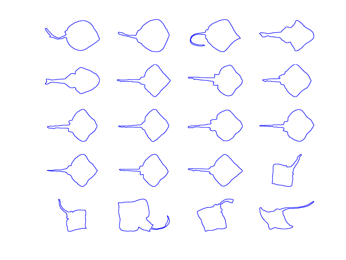

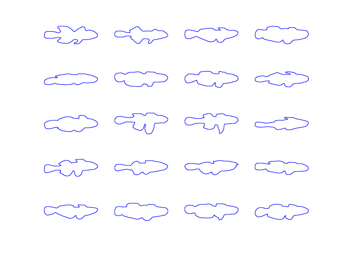
The first example, shown in Fig. 9, reveals that the confidence regions are wider in the portions of the shape in which there is more variability in the sample. Here, the bands are thicker in the regions corresponding to the tail and the top and bottom of the front section of the stingray, where the variability is the greatest. Secondly, samples with less variability result in narrower confidence regions. This can be seen by comparing Figs. 9 and 10. It is easy to see that there is less overall variability in the shapes of the contours of the wormfish than there is for the stingrays, which is reflected in the widths of the confidence regions. Furthermore, the effect of sample size on the confidence regions is clearly displayed in Fig. 11. As should be expected, the confidence region constructed using 88 observations is substantially thinner than that constructed using just 20 observations.

(a) (b)


In addition to being able to obtain sensible and intuitive results, the processing time needed to compute bootstrap confidence regions for the VW extrinsic mean is small compared to doing the same using the elastic framework for the analyzing the shape of planar curves. The higher computational cost is due to a combination of the intrinsic analysis and the elastic representation. The calculation of an intrinsic mean requires the use of an iterative algorithm. The square-root elastic framework of Joshi et al. (2007) [20] adapts the algorithm of Klassen et al. (2004) for arc-length parametrized curves by inserting a reparametrization step at each iteration. This reparametrization step requires the use of either a dynamic programming algorithm or a gradient descent approach. These time-consuming steps are repeated a number of times during the calculation of the intrinsic mean, which, when obtaining a bootstrap confidence region, results in the computational cost being further compounded. As an example, this methodology was performed on a sample of hand gestures representing the letter “L” using the concepts of elastic shape representation, as described in Joshi et al. (2007) [20], and our methodology. The resulting confidence regions are given in Fig. 12. Using MATLAB on a machine running Windows XP on an Intel Core 2 Duo processor running at 2.33 GHz, these computations required 47.9 hours for the elastic method and only 47.5 seconds for ours. The difference in the size of the contours displayed in Fig.12 is due to the approaches using different methods for normalization. While we scale the complex vector denoting the coordinates for the contour at the sampled times to have a norm of 1, the square-root elastic framework scales curves to have unit length. While both methods perform well at producing estimates for mean shape and providing bootstrap confidence regions, our approach is far more computationally efficient. For a more detailed account of the advantages of extrinsic analysis of data on manifolds, especially for obtaining bootstrap confidence regions, see also Bhattacharya et al.(2012)[7].
(a) (b)


9 Discussion
In this paper, we have described how to address the neighborhood hypothesis for one population mean on a Hilbert manifold. This first paper on data analysis on a Hilbert manifold opens up a new area for data analysis of infinite dimensional objects that can not be represented on a Hilbert space. This is a rich domain for further study, with potential extensions and techniques coming from recent advances in statistics on finite dimensional manifolds and data analysis on infinite dimensional Hilbert spaces. Regarding applications in shape analysis, while our theory and computational methodology leads to the estimation of the extrinsic mean direct similarity shapes of planar contours, this approach could be extended further to any infinite configurations in the Euclidean plane, including 1-dimensional CW-complexes and planar domains, given that the plane is separable. For example, one may consider shapes of edge maps obtained from gray-level images. In these cases, the problem of properly matching becomes much more difficult because, not only do points on a given edge from one image need to be matched to corresponding points on the corresponding edge in another image, but each edge in an image must be matched to the corresponding edge in another image, as well.
Additionally, we have only considered inference techniques for one-sample problems. While two-sample and multi-sample procedures may be more practical for many data analysis purposes, both the one-sample neighborhood hypothesis test and the non-pivotal nonparametric bootstrap confidence regions are useful nonparametric techniques for the estimation of the extrinsic mean shape for planar contours. In addition, they serve as an important first step towards the development and/or adapting of the desired two-sample and multi-sample procedures.
Furthermore, it should be noted that planar contour data carries with it innate difficulties that can be challenging to account for in the data analysis described in this paper. First, it is important to maintain a consistent camera position with respect to the object of interest to ensure that direct similarity shape analysis is appropriate. Otherwise, it may be more appropriate to consider projective shape analysis instead.
Finally, planar contours may commonly depict images of 3D objects. In the case that the object is relatively flat, such as with the stingrays in the example here, a slight shift in the camera angle may not result in a substantial change in the contour obtained from the digital image. However, for other 3D objects, such as the dogs and hand gestures, a slight shift may result in a drastic change in the form of the associated contour, which is an issue that has largely been ignored in the literature. In such cases, neither planar direct similarity shape nor planar projective shape may be an adequate descriptor for analyzing the contour data. Because of these issues, it is important to take great care with planar shape analysis of contours that arise from images of 3D solid objects. In such cases, where there is an absence of additional information on the scenes pictured, this care can help to ensure that a meaningful analysis can be conducted.
Acknowledgement
We are grateful to the organizers of the Analysis of Object Data program 2010/2011 at SAMSI, and, in particular, to Hans Georg Mller and to James O. Ramsey for useful conversations on infinite object data analysis regarded as data analysis on Hilbert manifolds. Thanks also to Rabi N. Bhattacharya and John T. Kent for discussions on the subject and to Ben Kimia and Shantanu H. Joshi for providing access to the silhouette data library.
References
- [1] Amaral, G. J. A. ; Dryden, I. L.; Patrangenaru, V. and Wood, A.T.A. (2010). Bootstrap confidence regions for the planar mean shape. Journal of Statistical Planning and Inference. 140, 3026-3034.
- [2] Azencott, R. (1994). Deterministic and random deformations ; applications to shape recognition. Conference at HSSS workshop in Cortona, Italy.
- [3] Azencott, R.; Coldefy, F. and Younes, L. (1996). A distance for elastic matching in object recognition Proceedings of 12th ICPR (1996), 687–691.
- [4] Bandulasiri, A.; Bhattacharya, R.N. and Patrangenaru, V. (2009) Nonparametric Inference for Extrinsic Means on Size-and-(Reflection)-Shape Manifolds with Applications in Medical Imaging. Journal of Multivariate Analysis. 100 1867-1882.
- [5] Bandulasiri A. and Patrangenaru, V. (2005). Algorithms for Nonparametric Inference on Shape Manifolds, Proc. of JSM 2005, Minneapolis, MN, 1617-1622.
- [6] Bhattacharya A. and Bhattacharya, R. N. (2008). Statistics on Riemannian Manifolds: Asymptotic Distribution and Curvature. Proceedings of the American Mathematical Society 136. 2957-2967.
- [7] Bhattacharya, R.N; Ellingson, L; Liu, X; Patrangenaru, V; and Crane, M. (2012) Extrinsic Analysis on Manifolds is Computationally Faster than Intrinsic Analysis, with Application to Quality Control by Machine Vision. To appear in Applied Stochastic Models in Business and Industry.
- [8] Bhattacharya, R.N. and Patrangenaru, V. (2003). Large sample theory of intrinsic and extrinsic sample means on manifolds-Part I,Ann. Statist. 31, no. 1, 1-29.
- [9] Bhattacharya, R.N. and Patrangenaru, V. (2005). Large sample theory of intrinsic and extrinsic sample means on manifolds- Part II, Ann. Statist., 33, No. 3, 1211- 1245.
- [10] Dauxois, J., Pousse, A. and Romain, Y. (1982). Asymptotic theory for the principal component analysis of a vector random function: some applications to statistical inference. J. Multivariate Anal. 12, 136–154.
- [11] Efron, B. (1979) Bootstrap methods: another look at the jackknife. it Ann. Statist. 7, No. 1, 1–26.
- [12] Fréchet, M. (1948). Les élements aléatoires de nature quelconque dans un espace distancié. Ann. Inst. H. Poincaré 10, 215–310.
- [13] Gaines, G. (2012). Random perturbation of a self-adjoint operator with a multiple eigenvalue. Dissertation. Department of Mathematics and Statistics, Texas Tech University.
- [14] Grenander, U. (1993). General Pattern Theory. Oxford Univ. Press.
- [15] Goodman, N. R. (1963). Statistical analysis based on a certain multivariate complex Gaussian distribution. (An introduction) Ann. Math. Statist. 34, 152–177.
- [16] Hall, P. (1992). The bootstrap and Edgeworth expansion. Springer Series in Statistics, New York.
- [17] Hall, P., Mller, H.-G., Wang, J.-L. (2006). Properties of principal component methods for functional and longitudinal data analysis. Ann. Statist. 34, 1493–1517.
- [18] Huckemann, S. and Ziezold, H. (2006). Principal component analysis for Riemannian manifolds, with an application to triangular shape spaces. Adv. in Appl. Probab. 38, no. 2, 299–319.
- [19] Huckemann, S. and Hotz, T. (2009). Principal component geodesics for planar shape spaces. J. Multivariate Anal. 100, no. 4, 699–714.
- [20] Joshi S.; Srivastava, A. ; Klassen, E. and Jermyn, I. (2007). Removing Shape-Preserving Transformations in Square-Root Elastic (SRE) Framework for Shape Analysis of Curves. Workshop on Energy Minimization Methods in CVPR (EMMCVPR). August.
- [21] Kaziska, D. and Srivastava, A. (2007). Gait-Based Human Recognition by Classification of Cyclostationary Processes on Nonlinear Shape Manifolds, JASA, 102(480): 1114-1124.
- [22] Kendall, D.G.; Barden, D.; Carne, T.K. and Le, H. (1999). Shape and Shape Theory. Wiley, New York.
- [23] Kendall, D.G. (1984), Shape manifolds, Procrustean metrics, and complex projective spaces. Bull. London Math. Soc. 16 81-121.
- [24] Kent, J.T. (1992), New directions in shape analysis. The Art of Statistical Science, A Tribute to G.S. Watson, 115–127. Wiley Ser. Probab. Math. Statist. Probab. Math. Statist., Wiley, Chichester, 1992.
- [25] Kimia, Ben. A Large Binary Image Database. http://www.lems.brown.edu/ dmc/
- [26] Klassen, E.; Srivastava, A. ; Mio, W. and Joshi, S. H. (2004). Analysis of Planar Shapes Using Geodesic Paths on Shape Spaces, IEEE Transactions on Pattern Analysis and Machine Intelligence 26 372 - 383.
- [27] Kume, A. and Le, H. (2003). On Fréchet means in simplex shape spaces. Adv. in Appl. Probab. 35 , 885–897.
- [28] Kume, A. and Le, H. (2000). Estimating Fréchet means in Bookstein’s shape space. Adv. in Appl. Probab. 32 , 663–674.
- [29] Lang, S. (1986) Differential manifolds. Springer, New York.
- [30] Le, H. (2001). Locating Fréchet Means with Application to Shape Spaces . Advances in Applied Probability, 33. 324–338.
- [31] Le, H. and Kume, A. (2000). The Fréchet Mean Shape and the Shape of the Means. Advances in Applied Probability, 32. 101-113
- [32] Le, H. and Kume, A.(2000). The Fréchet mean shape and the shape of the means. Adv. in Appl. Probab. 32 , 101–113.
- [33] Love, M. (1977). Probability Theory(fourth ed.) Springer-Verlag, Berlin.
- [34] Michor, P. W. and Mumford, D. (2004). Riemannian Geometries on Spaces of Plane Curves. Journal of the European Mathematical Society, 8, 1 - 48.
- [35] Mardia, K.V. and Patrangenaru, V. (2001) On affine and projective shape data analysis. In “Functional and Spatial Data Analysis”. Proceedings of the 20th LASR Workshop, edited by K.V. Mardia& R.G. Aykroyd , Leeds University Press, Leeds, 39–45.
- [36] Mio, W. and Srivastava, A. (2004). Elastic-String Models for Representation and Analysis of Planar Shapes. Proceedings of the IEEE Computer Society International Conference on CVPR.10–15.
- [37] Mio, W.; Srivastava, A. and Klassen, E. (2004)Interpolation by Elastica in Euclidean Spaces.Quarterly ofApplied Math. 62, 359 - 378 .
- [38] Mio, W.; Srivastava, A. and Joshi, S. (2007). On the Shape of Plane Elastic Curves. International Journal of Computer Vision, 73, 307–324.
- [39] Mller, H.-G., Stadtmller, U. and Yao, F. (2006). Functional variance processes. J. Amer. Statist. Assoc. 101 1007–1018.
- [40] Munk, A. and Dette, H. (1998) Nonparametric comparison of several regression functions: exact and asymptotic theory. Ann. Statist. 26, 2339-2368.
- [41] Munk, A.; Paige, R.; Pang, J. ; Patrangenaru, V. and Ruymgaart, F. H.(2008). The One and Multisample Problem for Functional Data with Applications to Projective Shape Analysis. J. of Multivariate Anal. . 99, 815-833.
- [42] Patrangenaru, V. (1998). Asymptotic Statistics on Manifolds, PhD Dissertation Indiana University.
- [43] Patrangenaru, V., Liu, X. and Sugathadasa, S. (2010). Nonparametric 3D Projective Shape Estimation from Pairs of 2D Images - I, In Memory of W.P. Dayawansa. Journal of Multivariate Analysis. 101, 11-31.
- [44] Ramsay J. O. and Silverman, B. W. ( 2005). Functional Data Analysis, Springer Series in Statistics, Springer, 2nd edition.
- [45] Sebastian, T.B. ; Klein, P.N. and Kimia,B.B. (2003). On Aligning Curves. IEEE Trans. Pattern Analysis and Machine Intelligence 25, no. 1, 116–125.
- [46] Small, C. G. (1996). The Statistical Theory of Shape, Springer-Verlag, New York.
- [47] Srivastava, A. and Klassen, P.E. (2002). Monte Carlo extrinsic estimators for manifold-valued parametersIEEE Transactions on Signal Processing. 50, 299-308.
- [48] Srivastava, A. ; Joshi, S. Mio, W. and Liu, X. (2005). Statistical Shape Analysis: Clustering, Learning and Testing. IEEE Trans. Pattern Analysis and Machine Intelligence, 27. 590–602.
- [49] Younes, L. (1998). Computable elastic distance between shapes. SIAM Journal of Applied Mathematics, 58, 565-586.
- [50] Younes, L. (1999). Optimal matching between shapes via elastic deformations. Journal of Image and Vision Computing, 17, 381-389.
- [51] Younes, L.; Michor, P. W.; Shah, J. and Mumford, D. (2008). A metric on shape space with explicit geodesics. Rend. Lincei Mat. Appl. 19 25-57.
- [52] Zahn, C. T. and Roskies. (1972). Fourier Descriptors for Plane Closed Curves. IEEE Tras. Computers 21 269-281.
- [53] Ziezold, H. (1998). Some aspects of random shapes. (English summary). Numbers, information and complexity (Bielefeld, 1998), 517–523, Kluwer Acad. Publ., Boston, MA.
- [54] Ziezold, H. (1994). Mean figures and mean shapes applied to biological figure and shape distributions in the plane. Biometrical J. 36, no. 4, 491–510.
- [55] Ziezold, H. (1977). On expected figures and a strong law of large numbers for random elements in quasi-metric spaces. Transactions of the Seventh Prague Conference on Information Theory, Statistical Decision Functions, Random Processes and of the Eighth European Meeting of Statisticians, Vol. A, 591-602. Reidel, Dordrecht.