Improving Electro-Weak Fits with TeV-scale Sterile Neutrinos
Abstract
We study the impact of TeV-scale sterile neutrinos on electro-weak precision observables and lepton number and flavour violating decays in the framework of a type-I see-saw extension of the Standard Model. At tree level sterile neutrinos manifest themselves via non-unitarity of the PMNS matrix and at one-loop level they modify the oblique radiative corrections. We derive explicit formulae for the parameters in terms of the neutrino masses and mixings and perform a numerical fit to the electro-weak observables. We find regions of parameter space with a sizable active-sterile mixing which provide a better over-all fit compared to the case where the mixing is negligible. Specifically we find improvements of the invisible -decay width, the charged-to-neutral-current ratio for neutrino scattering experiments and of the deviation of the boson mass from the theoretical expectation.
Keywords:
Type-I see-saw mechanism, sterile neutrinos, invisible Z decay width, oblique corrections, non-unitaritypacs
14.60.St, 14.60.Pq, 13.15.+g, 12.15.LkI Introduction
The Standard Model (SM) is extremely successful and has passed numerous experimental tests. Moreover the last missing piece, the Higgs particle, has recently likely been seen by the ATLAS and CMS collaborations [1, 2]. On the other hand, the SM is for a number of theoretical reasons incomplete. It also does not explain three known experimental facts, namely the tiny active neutrino masses, the baryon asymmetry of the Universe and the existence of dark matter. A simple yet elegant way to solve two or even all of these problems is to supplement the SM by three singlets:
| (1) |
where are Majorana fields, are the lepton doublets, is the conjugate of the Higgs doublet, and are the corresponding Yukawa couplings.
This is a small modification of the SM, also because so far the principles which select the fermionic representations in a given theory are (besides for anomaly conditions) unknown. Nevertheless, this modification allows to accommodate those three experimental facts: First, after breaking of the electro-weak symmetry the active neutrinos acquire masses via the type-I see-saw mechanism [3, 4, 5, 6]. Second, within the same setup the observed baryon asymmetry of the Universe can be naturally explained by leptogenesis [7]. According to this scenario the lepton asymmetry which is produced by the heavy neutrinos is converted into the baryon asymmetry by anomalous electro-weak processes [8, 9, 10]. Depending on the values of the masses and couplings in (1) the generation of the asymmetry proceeds either through decays [11, 12, 13, 14, 15, 16, 17, 18, 19, 20, 21, 22, 23] or via oscillations of the heavy neutrinos [24]. The extension of the SM spectrum by sterile neutrino states may even provide a solution to the third problem, since sterile neutrinos are a perfect dark matter candidate (see e.g. [25, 26, 27, 28, 29, 30, 31, 32]). A further possible implication of sterile neutrinos is a modified active neutrino flux in reactor experiments [33]. This could explain the observed reduced electron antineutrino fluxes [34].
Note that the addition of singlets to the SM has actually important consequences. Not only are there many new parameters, but also the global symmetries are changed, since lepton number is broken. Furthermore the single scale of the SM, namely the electro-weak VEV, is amended by the new mass scales . Within the type-I see-saw the sterile neutrinos pick up masses proportional to and these could in principle have any value which is not excluded by experiment. It is therefore interesting to study implications of sterile neutrinos assuming any mass. Some effects exist even for ultra heavy sterile neutrinos, while some are only phenomenologically important for not so heavy states, which are in the mass range of several TeV or lower.
The existence of Majorana neutrinos has well known consequences on the phenomenology below the electro-weak scale. In particular, the new states can contribute to the amplitude of the neutrinoless double-beta decay [35, 36, 37, 38, 39] and induce rare charged lepton decays [40, 41]. Furthermore, they can affect the electro-weak precision observables (EWPOs) via tree-level as well as loop contributions and thus provide an explanation for anomalies in the experimental data. In particular, the tree-level effects result in non-unitarity of the active neutrino mixing matrix [40] and lead to a suppression of the invisible -decay width. This is in agreement with the long standing fact that the LEP measurement of the invisible -decay width is two sigma below the value expected in the SM [42]. Furthermore the neutral-to-charged-current ratio in neutrino scattering experiments can be changed thus providing an explanation for the NuTeV anomaly [43]. Also a slight shift of the boson mass from the value derived from other SM parameters is induced, reducing the tension between the input parameters of the electro-weak fit and the experimentally observed value [44]. These electro-weak observables are affected not only at tree-level but also by loop effects. The latter can be taken into account in the form of the oblique corrections and can partially ‘screen’ the tree-level contributions, as we will see later. The impact of oblique corrections on models with non-universal neutrino gauge coupling has been studied in [45, 46, 47]. In these works the tree-level effects (, and ) and oblique (, and ) corrections have been treated as independent parameters. However, in the model described by the Lagrangian (1) they are functions of the Majorana masses and Yukawa couplings and are therefore not independent.
Encouraged by the fact that sterile neutrinos are very well motivated we study their phenomenological impact in this paper. Specifically we consider TeV-scale sterile neutrinos with a sizable active-sterile mixing and determine their over-all contributions to the EWPOs and to indirect detection experiments in the framework of the see-saw type-I extension of the SM. In contrast to the previous studies we derive expressions for the -parameters in terms of the masses and mixing angles of the Majorana neutrinos, thus all quantities effecting the observables are functions of the parameters in (1). Our approach is therefore completely self-consistent. In Sec. II we discuss the influence of heavy Majorana neutrinos on the phenomenology below the electro-weak scale and provide expressions for the -parameters. Next we perform in Sec. III a likelihood fit to the EWPOs taking into account up-to-date experimental constraints including neutrino oscillation data and limits from the non-observation of rare charged lepton decays and neutrinoless double-beta decay. We find that TeV-scale sterile neutrinos improve the overall fit by bringing the invisible -decay width, the charged-to-neutral current ratio for neutrino scattering and the boson mass in agreement with the experimentally observed values within the experimental precision. The best-fit regions provide testable experimental signatures. For the normal- and quasi-degenerate light neutrino mass spectra we find that decay rates are close to the current experimental sensitivities. For the inverted hierarchy the mass region is such that part of the parameter space can be tested at the LHC after the 14 TeV upgrade. Finally, in Sec. IV we summarize the obtained results and present our conclusions.
II Observables
The heavy neutrino fields in (1) are SM singlets and do not participate in the gauge interactions. However, the breaking of the electroweak symmetry induces a neutrino Dirac mass term. The mass eigenstates obtained by diagonalization of the full mass matrix couple to the and bosons. Expressed in terms of the mass eigenstates the corresponding part of the Lagrangian takes the form
| (2) |
where denote the charged leptons, denote the light (for ) as well as heavy (for ) neutrinos, and is the full unitary neutrino mixing matrix. To give masses to at least two active neutrinos, as required by oscillation experiments, we need two or more heavy neutrinos, i.e. , but otherwise is unconstrained. Below we review the phenomenology of (2) together with the corresponding up-to-date experimental results.
Lepton-flavor violating decays. In the scenario under consideration the branching ratio of decay is given by [48]
| (3) |
where and the loop function is defined by
Note that we use to denote the masses of both light and heavy neutrinos. Since the masses of the active neutrinos are very small we can neglect them in the loop integral, . Using unitarity of the full mixing matrix we then find
| (4) |
The recent limit on this branching ratio obtained by the MEG collaboration [49] is
| (5) |
at confidence level. From (4) and (5) we can infer bounds on the products of the mixing elements and . An analogous relation also exists for the decay. However, the corresponding experimental constraints are much weaker and will not be considered here.
Neutrinoless double-beta decay. Neutrinoless double-beta decay constrains the effective mass of the electron neutrino . The latter receives contributions from the light as well as from the heavy mass eigenstates [35]:
| (6) |
For masses of the heavy neutrinos in the TeV range one can use an approximation: , where GeV and depends on the decaying isotope under consideration [39, 50]. A conservative bound, eV, has been recently obtained by EXO collaboration [51].
Unitarity and lepton universality violation. For the following analysis it is convenient to represent in the form
| (7) |
The matrix describes the active-sterile mixing. An obvious consequence of a nonzero active-sterile mixing is that the PMNS matrix is no longer exactly unitary [40]. The deviation from unitarity can be parameterized by
| (8) |
In general the quantities , and are not equal. In other words, there is also a violation of lepton universality. Experimental bounds on linear combinations of the read [45]
| (9a) | |||
| (9b) | |||
| (9c) | |||
The stringent experimental bound on the branching ratio implies that either or is negligible in (9). For a recent study of lepton universality violation in Pion and Kaon decays in the presence of sterile neutrinos consult [52].
Heavy neutrinos at colliders. Heavy singlet Majorana fermions have been searched for at the LEP and LHC colliders, see [53, 54] for a review. The searches were based on the production of the heavy state due to a considerable mixing to the active neutrinos.
At LEP the heavy neutrino could be produced in annihilation, , via -channel -exchange as well as via -channel -exchange. The produced Majorana neutrinos then rapidly decay via the weak neutral or charged currents: and . A search for heavy neutrinos with masses up to GeV has been performed by the L3 and Delphi collaborations using the latter decay channel with decaying into hadrons [55, 56]. The experimental signature of these events would be one isolated electron plus hadronic jets.
New limits on the active-sterile mixing for the heavy neutrino masses up to 210 GeV have been obtained recently by the CMS collaboration [57] using a dilepton decay channel with two leptons of equal charge and flavour plus jets, see Fig. 1.
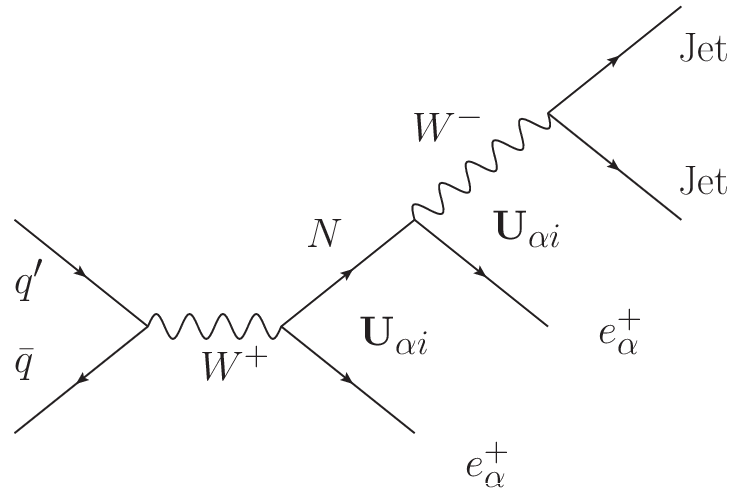
Violation of lepton number in this process occurs due to the Majorana nature of the sterile neutrino. For large Majorana masses the square of the momentum transfer in the propagator of the intermediate neutrino can be neglected and the production cross section depends on the combination . Assuming that only one of the heavy neutrinos couples to the electron with a strength it has been estimated in [59] that after the LHC upgrade to TeV this channel can be used to search for Majorana neutrinos with masses up to roughly 800 GeV. For these parameters we get TeV-1 and one event per is expected. Even though this is a very weak statistical signal it has been noted that in the highest mass region the leptons are emitted back to back providing a very clean signature and allowing for an excellent background suppression. If the luminocity of is reached one can hope to find the heavy neutrinos even if the above defined combination of the mixings and masses is as small as TeV-1.
A possible way of testing even higher mass ranges is to study electron-proton collisions where the dominant detection channel is with the Majorana neutrino as an intermediate state. In [60] it has been estimated that at an electron-positron collider with a center of mass energy TeV mass ranges up to 1.5 TeV can be tested.
Non-unitarity in neutrino oscillations. The standard oscillation formula assumes unitarity of the PMNS matrix , which is violated in the model under consideration. The non-unitarity of will manifest in a modified oscillation probability formula [40], which in particular includes a zero-length effect [61]:
| (10) |
Being of second order in for this effect is strongly suppressed. As discussed by a number of authors, see [40] and references therein, the probabilities do not add up to unity. At non-zero distances the non-unitarity effects are linear in [62] and may affect the results of global fits. For the purposes of this work we will use the best-fit results for the light neutrino parameters obtained in a unitary fit as an input, see [63]. The order corrections to the parameters of the active neutrinos will be computed using (20). At the end, when comparing the corrected values to the results of the unitary fit in [63] we find agreement within the one sigma intervals. The values are also consistent with the one sigma intervals obtained in a non-unitary fit [40]. Furthermore, we have checked that our results are not sensitive to changes of the active neutrino parameters within their experimental errors, which justifies our procedure.
Electroweak precision observables. An important consequence of non-unitarity is that the couplings of the light neutrinos to the and bosons are suppressed with respect to their SM values. Taking this effect into account we find that the invisible -decay width is suppressed:
| (11) |
This means that the ‘effective number of neutrinos’ measured in the -decay is slightly less than three, which is qualitatively agreeing with the LEP results [42].
| EWPO | Theory (Standard Model) | Experiment |
|---|---|---|
| (MeV) | ||
| (GeV) |
Similarly, cross-sections of the charged- and neutral-current neutrino scatterings on quarks are also affected:
| (12a) | ||||
| (12b) | ||||
The stronger relative suppression of the neutral current interactions can be observed in experiments measuring ratios of the corresponding cross sections. In particular, it is qualitatively consistent with the results of the NuTeV experiment [66, 67, 68, 69]. Another important consequence of non-unitarity is that – the Fermi constant measured in the muon decay – is not equal to the Fermi constant measured in experiments with semi-leptonic processes, but
| (13) |
Since the muon decay width is used as an input in the SM fits, this modification influences many observables and has been used in [40] to obtain bounds on the active-sterile mixing. However, as argued in [45, 46], the impact of the heavy neutrinos is not limited to the above discussed tree-level effects. Heavy neutrinos contribute to the self-energies of the and bosons and therefore modify their propagators. These loop effects can be described in terms of the parameters [70]. A more detailed description of the oblique correction formalism is presented in Appendix A, while the calculations are shown in Appendix B. Combining the tree-level and one-loop contributions one obtains [45, 46]
| (14a) | ||||
| (14b) | ||||
| (14c) | ||||
| (14d) | ||||
| (14e) | ||||
| (14f) | ||||
Comparing (11) and (14b) we see that the first line in the latter equation is the leading-order expansion of the former one and that the loop corrections enter through the and parameters.
Cancellation mechanism. Since and are related to derivatives of the and boson self-energies whereas is proportional to a difference of the two, usually and are subdominant in comparison to . If is neglected then (14a) and (14c) depend on the same combination of tree-level and one-loop corrections, , where is the fine structure constant. The reason is that in this approximation the shift of these observables is solely due to a shift in [46]. It has been argued in [40] that a shift in has dramatic effect on the electro-weak observables and thus and are strongly constrained. However, as follows from (14), if the tree-level and radiative contributions are of a similar size the shift induced by the tree-level effects can be ‘screened’ by a sizable negative parameter. Typically, most of the SM extensions result in a positive parameter. Therefore, it was assumed in [46] that the Higgs mass is much larger than the used reference value, GeV. However, interpreting the recent discovery of the ATLAS and CMS collaborations as the SM Higgs, this option is excluded.
Majorana neutrino contribution to the parameters. Here we argue that the screening can be realized without invoking any new physics beyond that already introduced in (1). As demonstrated in [71] for a model with a single heavy neutrino, in a certain range of the parameter space Majorana neutrinos can generate a negative contribution to the parameter. In the model with heavy neutrinos we find
| (15) |
where denote masses of the charged leptons. To shorten the notation we have introduced
| (16) |
where , , and are the usual one-loop functions [72], and . Details of the calculation can be found in Appendix B. Note that although the loop functions are divergent and contain an arbitrary scale , their combination (15) is finite and independent of . This can be shown using the unitarity of the full mixing matrix and the type-I see-saw condition with . Therefore, to compute (15) one can simply drop the terms in the expansion of the loop functions and evaluate the remaining integrals numerically or analytically. As indicated in (15), the T parameter is a sum of the SM and new contributions. The SM contribution can be obtained from (15) by setting the active neutrino masses to zero and taking into account that and is unitary in the SM:
| (17) |
This expression is also finite. Note that the PMNS matrix does not appear in (17) since the mixing becomes unphysical for massless neutrinos. The parameter reads
| (18) |
where and is defined in the same way. The SM contribution, , is calculated analogously to . For the parameter we obtain
| (19) |
For a single generation Eqs. (15), (18) and (19) reduce to the expressions derived in [71]. The observation that the heavy neutrinos can ‘screen’ the tree-level contributions by generating a negative parameter together with the explicit formulae for the constitutes one of the main results of the present work.
III Fit to the observables
In this work we investigate the impact of TeV-scale sterile neutrinos with a sizable active-sterile mixing on the physics below the electro-weak scale in the framework of the see-saw type-I extension of the SM. In the see-saw limit the active-sterile mixing is of order . On the other hand, the see-saw formula for the mass matrix of the light neutrinos reads . Comparing the two expressions we conclude that for a large active-sterile mixing the smallness of the active neutrino masses can not be explained by the scale suppression. Instead, contributions from different heavy states have to mutually cancel. To ensure the cancellation more than one sterile neutrino is needed. As already mentioned above, two heavy neutrinos are required to ensure that at least two of the light neutrinos are massive. We have also seen that the mixing to either the electron or the muon neutrino has to be strongly suppressed to be compatible with the current bounds. Combined together, the two conditions imply that the cancellation is only possible for . We consider in this paper, which arises naturally in the framework of many left-right symmetric or GUT models.
For both and are matrices which can be written in the form [73]:
| (20a) | ||||
| (20b) | ||||
with being an arbitrary complex orthogonal matrix, the unitary matrix diagonalizing , the diagonal mass matrix of the heavy neutrinos and that of the light neutrinos. The entries of are extracted from a global fit to atmospheric, reactor and solar neutrino oscillation data. Note that a possible non-unitarity of is neglected in usual global fits, i.e. it is assumed that . The resulting best fit values and ranges for the three mixing angles and the Dirac CP-phase11 1 The one sigma best fit region for the CP-phase was determined in [74] to be . However, the choice of the CP-phase has no significant impact on our results. read (see e.g. [63])
| (21a) | ||||
| (21b) | ||||
| (21c) | ||||
| (21d) | ||||
whereas the two Majorana phases are unknown and will be set to zero in the fit. The remaining degrees of freedom are the three masses of the heavy neutrinos and the entries of the matrix . The latter can be parametrized by three complex angles. The freedom of choosing may be used to suppress the active-sterile mixing for one active neutrino flavour. Whether this suppression is possible or not depends on the structure of the light neutrino mass matrix, as can be inferred from (20).
| NH | IH | QD | |
|---|---|---|---|
Since the absolute neutrino mass scale is unknown at present, we consider three possible neutrino mass spectra called NH, IH and QD which are defined in Table 2. In the case of the QD mass spectrum, the masses are constrained by the recent WMAP bound eV [75]. For the numerical example in the QD case we use eV.
The minimization of the function is performed with a Monte Carlo method described in Appendix D. Let us note that this method can not find continuous solutions but falls randomly in the good fit points. For a given point in the parameter space we compute the branching ratio and the effective electron neutrino mass , relevant for the . For most of the points with a sizable active-sterile mixing one of these bounds is violated. To take the two bounds into account in the analysis we define
| (22a) | ||||
| (22b) | ||||
where and are the theoretical predictions computed at the chosen point of the parameter space, whereas and are the corresponding experimental upper bounds. We use the theta step function to restrict the contributions to the total to cases when the theoretical prediction exceeds the one sigma exclusion limit. Additionally, we check whether the universality constraints, see Eq. (9), are fulfilled. Finally, we compute the parameters and the corrected values of the electro-weak precision observables , see Eq. (14). The corresponding value is calculated using
| (23) |
where denotes the predictions of the SM, are the theoretical errors and are the experimental errors, see Table 1. Note that we neglect off-diagonal elements of the covariance matrix in these contributions. The total is given by the sum of (22) and (23).
Using this definition we find that for points with negligibly small active-sterile mixing (‘natural’ see-saw) ( for the QD mass spectrum). This relatively large value of is induced primarily by the anomalies in the invisible -decay width, the NuTeV results and the deviation of the boson mass from the SM expectation. The slightly higher value for the QD mass spectrum stems from the fact that neutrino masses of the order of eV induce an effective electron neutrino mass comparable to the current upper bound.
To get a rough estimate of the goodness of the fit we compute the ratio of to the number of degrees of freedom. The and parameters are always very small and can be neglected in the fit. Therefore, the initial set of free parameters, the three masses and three complex angles, maps to four quantities: , , and . Since we fit six observables and two constraints, the number of degrees of freedom is and for the case of negligible active-sterile mixing. Below we perform a fit for each of the three light neutrino mass spectra to all EWPOs and constraints. In the following in all plots the full is presented.
For all mass spectra we will show how the EWPOs in the best-fit regions are shifted with respect to the SM predictions. The question will be addressed whether a direct detection or an indirect signal of the new states is feasible in near future. To study this possibility the branching ratio, the decay rate and the strength of a collider signal will be estimated.
Normal mass hierarchy. Let us first consider the normal mass hierarchy of the light neutrinos. The branching ratio is suppressed in particular if is small. As discussed above, if and are neglected then the boson leptonic decay width (14a) and the Weinberg angle (14c) depend on the same combination of tree-level and one-loop corrections, . The reason is that in this approximation the shift of these observables is solely due to a shift of with respect to .
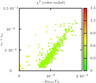
In Fig. 2 we show the fit to and the Weinberg angle only. The plot shows the (approximately) linear relation between and the parameter. The fact that the band does not start at the origin indicates that the two observables favour a slightly negative in general even in a different new physics model. This plot demonstrates how a negative value of the T parameter can screen the contributions of the neutrino mixing to the above mentioned observables. We will see that this cancellation mechanism is still at work when more observables are considered.
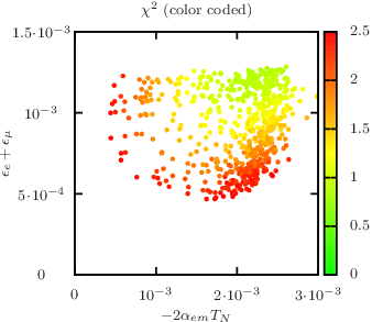
Large cancellations are present when the other EWPOs except the boson mass are taken into account. However, in this case the simple linear dependence is violated due to the necessity of fitting the other observables, see Fig. 3. The boson mass has been measured with a very high accuracy and a large negative would induce unacceptably large corrections to it. The fit excluding is of interest since an extended scalar sector appearing, for instance, in the type-I+II see-saw extension of the SM will shift the mass and might absorb the additional negative contribution restricted in the type-I see-saw.
Note that the following plots are two-dimensional projections of a multi-parameter scan and therefore points with rather different values of the color coded parameter can appear mixed on the plots.
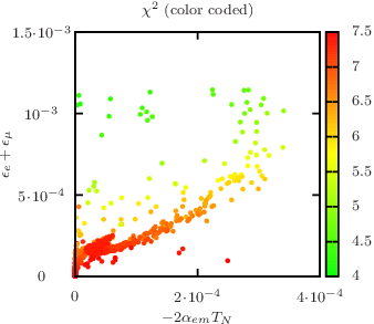
In Fig. 4 we show how the cancellation pattern changes if all observables in (14) are included. In this case for the best-fit points we have and a small negative is favored. The latter partially compensates the small positive contribution of to .
As can be inferred from Fig. 6, at the best-fit points at least one the Majorana neutrinos is relatively light, around one TeV,

and has a sizable coupling to at least one of the charged leptons, see Fig. 5. In other words, the current data favour the low-scale type-I see-saw with a considerable active-sterile mixing over the standard scenario (‘natural’ see-saw) where this mixing is negligible and the masses of the heavy neutrinos are close to the GUT scale. On the other hand, as can be seen in a different projection of the same plot in Fig. 6, heavy neutrinos with masses below TeV scale are also disfavoured. The reason is that for sizable active-sterile mixing in this mass range experimental bounds are more stringent.

As already mentioned above, for a sizable active-sterile mixing the cancellation of the contributions to the light neutrino masses imposes constraints on the mass spectrum of the heavy ones. Due to requirements of suppressed an active-sterile mixing pattern occurs where the first and third heavy mass eigenstates have comparable, sizable mixing to the active flavours while the mixing of the second is small. We find that the first and third heavy mass eigenstates have approximately equal masses whereas the mass of the remaining sterile neutrino is considerably larger. This mass pattern leads to a small negative parameter as discussed above.
At the best-fit points the deviation of the PMNS matrix from unitarity is of the order of
which is in excellent agreement with the bounds derived in [76]. This consistency check justifies our procedure and the applicability of the approximation in (20). The corresponding (largest) zero-length transition probability is . This value is too small to explain the current short-baseline anomalies [77] but might contribute to the observed discrepancies.
In Fig. 7 we demonstrate how the EWPOs in the considered scenario are shifted from the values expected in the SM towards the experimentally observed ones. At the chosen best-fit point and therefore the absolute improvement of the fit is leading to a . Some of the observables are shifted away from the experimentally measured value compared to the SM prediction. Nevertheless, they remain within the one sigma interval around the experimental results. In addition, observables for which the SM prediction is in tension with data are brought into the one sigma intervals around their experimental values. This leads to a global picture in which all observables agree on the one (or in the case of on the 1.2) sigma level with the experiments. This leads to a of order one.
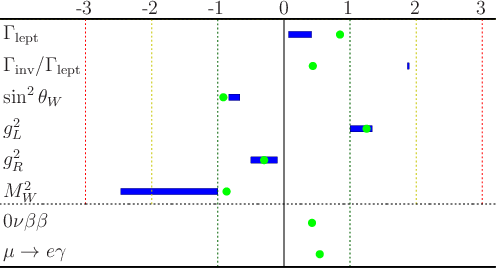
The improvement stems primarily from which leaves unaffected (and thus equal to ) but suppresses the invisible -decay width. Furthermore, shifts the boson mass towards the measured value. The NuTeV observables are not significantly changed. The last two rows in Fig. 7 present the ratios of the induced effective electron neutrino mass and the branching ratio to the corresponding experimental bounds.

It is interesting to note that for the normal mass hierarchy there are many points in the parameters space with values of these two quantities close to the threshold of the current experimental sensitivity, see Fig. 8. Here the predictions for the branching ratio and of the points in the parameter space with significant improvement of the are compared to current experimental limits. Knowing the masses of the heavy neutrinos and their couplings to the charged leptons we can also estimate the cross-section of the direct detection process depicted in Fig. 1. For all best-fit points the resulting value of turns out to be at most of the order of and thus beyond the LHC reach.
The branching ratio is also suppressed if is small. In this case we obtain a slightly worse best-fit value of which corresponds to . As compared to the previous case, in the best-fit points the invisible -decay width is less suppressed and the shift in the boson mass is smaller, see Fig. 9. On the other hand, is shifted towards the value measured by the NuTeV collaboration and thus brought in agreement with the data within the one sigma interval.
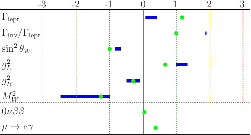
Inverted mass hierarchy. For the inverted mass hierarchy scenario only the option of negligible can be realized and results in best fit values of and . The EWPOs of the best-fit points are influenced such that the predicted invisible -decay width is brought within the one sigma interval to the experimental value, see Fig. 10. The boson mass is shifted in the right direction but less significantly than in the normal hierarchy scenario. On the other hand, is shifted towards the value measured by the NuTeV collaboration and brought in good agreement with the data.

As can be inferred from Fig. 11, both the effective electron neutrino mass and the branching ratio are in large parts of the parameter space close to the current experimental sensitivity.

Furthermore, for a small fraction of the best-fit points, see Fig. 12,

there is a chance of observing the heavy Majorana neutrinos at the LHC after the planned upgrade to TeV.
Quasi-degenerate mass spectrum. For the quasi-degenerate mass spectrum it is quite difficult to find points with sizable that pass the constraint. On the other hand, there are points with small and sizable and which satisfy the , neutrinoless double-beta decay and universality constraints. For the best-fit points leading to an improvement of and to . At the best-fit points the shift of the invisible -decay width is smaller than in the normal hierarchy scenario, but still the prediction moves into the one sigma interval of the observations. The shift in the boson brings prediction and experiment in excellent agreement, see Fig. 13. The neutrino scattering observable is not significantly influenced in comparison to the standard model expectation.

As can be inferred from Fig. 14 both the effective mass of the electron neutrino and branching ratio here can be close to the exclusion limit.

Note that the active neutrinos induce a sizable contribution to the effective electron neutrino mass in this case and can constructively or destructively interfere with the heavy neutrino contributions depending on the Majorana phases of the active neutrinos.
For all the best-fit points the resulting value of turns out to be at most of the order of and thus beyond the LHC reach.
It has been found that for all three mass spectra the current data favour a type-I see-saw with considerable active-sterile mixing over the a scenario where the mixing is negligible. For all three cases there are many points in the parameter space which generate signals in rare decay experiments close to the current sensitivities. For the IH a part of the parameter space can be tested at the LHC after the next upgrade.
IV Summary and outlook
In this work we have studied the impact of TeV-scale sterile neutrinos with a sizable active-sterile mixing on electro-weak precision observables and lepton number and flavour violating decays in the framework of the type-I see-saw extension of the SM. The active-sterile mixing can in particular improve the global fit and reduce some anomalies in the experimental data: first, it results in a decreased value of the invisible boson decay width, which is preferred by the current data; second, it slightly increases the mass of the boson and brings it in the one sigma interval around the observed value. Furthermore, in the case when is not suppressed, the model affects the charged-to-neutral current ratio for neutrino scattering and brings in agreement with the values observed by the NuTeV experiment.
In our analysis we have taken into account tree-level contributions of sterile neutrinos as well as their one-loop effects on gauge boson propagators. The tree-level contributions enter via non-unitarity of the PMNS mixing matrix, whereas the loop-contributions modify the propagators of the gauge bosons and can be taken into account in form of the parameters. The oblique corrections can play an important role. In particular we have demonstrated that a sizable negative parameter ‘screens’ the effect of tree-level non-unitarity on the Fermi constant. This cancellation mechanism can reconcile large active-sterile mixing with the current observations. As compared to previous analyses we have derived explicit formulae for the oblique corrections in terms of the Majorana masses and mixings and therefore studied a full and self-consistent model. We have performed a numerical fit to the electro-weak precision observables taking into account constraints from the non-observation of and neutrinoless double-beta decay processes as well as constraints on lepton non-universality. Since the active neutrino mass hierarchy is unknown at present, we have considered the cases of normal, inverted and quasi-degenerate mass spectra. In all three cases regions of the parameter space with a sizable active-sterile mixing provide a better overall fit to the data than regions where it is negligible. In other words, the current data favour the low-energy type-I see-saw with a considerable active-sterile mixing over the standard scenario (‘natural’ see-saw) where this mixing is negligible. Together with the derivation of expressions for the oblique corrections in the type-I see-saw this finding is one of the main results of the present work.
The is lowest for the normal hierarchy scenario and slightly higher for the inverted hierarchy and the case of the quasi-degenerate mass spectrum. We have also studied the experimental signatures of the best-fit points for each mass hierarchy. For all mass spectra the effective electron neutrino mass – the quantity relevant for the neutrinoless double-beta decay – reaches at many best-fit points values that are close to the sensitivity threshold of current experiments. The expected active-sterile mixing is of the order of in all three scenarios. The lightest sterile neutrino mass for normal- and quasi-degenerate mass spectra is around 2 TeV. This ranges might become accessible at electron-proton colliders with energies above 6 TeV. For the inverted hierarchy the Majorana masses can be as low as 300 GeV. Thus, given the predicted mixing, this scenario can be partially tested at the LHC after the 14 TeV upgrade.
The fit might improve in a type I+II see-saw extension of the SM, since the VEV of the additional Higgs triplet also contributes to the boson mass. Thus the negative parameter can be larger and the cancellation mechanism more efficient. This extension will be studied in a forthcoming paper.
Acknowledgements
The work of A.K. has been supported by the German Science Foundation (DFG) under Grant KA-3274/1-1 “Systematic analysis of baryogenesis in non-equilibrium quantum field theory”. J.S. acknowledges support by the IMPRS for Precision Tests of Fundamental Symmetries. The authors would like to thank M. Blennow, T. Schwetz , J. Heeck, J. Barry, W. Rodejohann and S. Antusch for helpful discussions.
Appendix A Oblique corrections
The formalism of oblique corrections was developed to study new physics which affects the observables only via corrections to the propagators of the gauge bosons [78, 79]. The Lorentz structure of the corresponding self-energies is
| (24) |
where . Since in the considered processes all external fermions are light, the contributions of the terms is proportional to and can safely be neglected. For the same reason, contributions of the box diagrams as well as the vertex corrections stemming from the new physics are negligible. Therefore, it is sufficient to consider only . The latter can be represented in the form
| (25) |
where . It follows from the Ward identity that which further constrains the number of independent quantities. It can be shown that for heavy new physics there are only three independent combinations of the above quantities that enter the expressions for the electro-weak observables [78]. These are denoted by , and and read [78, 71]:
| (26a) | ||||
| (26b) | ||||
| (26c) | ||||
The hats denote self-energies renormalized using the on-shell renormalization condition:
| (27) |
Explicit formulae for the renormalized self-energies in terms of the unrenormalized ones are [71]:
| (28a) | ||||
| (28b) | ||||
| (28c) | ||||
| (28d) | ||||
where
| (29) |
Substituting (28) into (26) and taking into account that we find:
| (30a) | ||||
| (30b) | ||||
| (30c) | ||||
Note that only for the parameter the expression in terms of the unrenormalized self-energies has the same form as in terms of the renormalized ones, compare (26b) and (30b).
Appendix B Calculation of S,T,U
To evaluate the contribution of Majorana neutrinos to the parameters defined in Appendix A we need to calculate the self-energies entering (30).

Only charged leptons contribute to and , see Fig. 15. The resulting self-energies are the same as in the SM:
| (31a) | ||||
| (31b) | ||||
where denote the masses of the charged leptons. To shorten the notation in (31) we have introduced
| (32) |
where , , and are the usual one-loop functions [72], and . The one-loop contribution of the charged leptons and neutrinos to is presented in Fig. 16.

Note that due to the nonzero active-sterile mixing the heavy neutrinos can also run in the loop. In position space the resulting self-energy is given by:
| (33) |
Since we deal with Majorana fermions, to evaluate (33) it is convenient to use the two component notation for the spinors, see Appendix C for more details. The self-energy then takes the form:
| (34) |
where denotes left-handed component of the charged-lepton field in the two-component notation. To evaluate (34) we need to consider all possible contractions of the field operators. Using the Fourier-representation of the propagators we obtain:
| (35) |
Note that since only the left-handed component of the charged field runs in the loop, only ‘kinetic’ contraction is possible. This is reflected by the fact that the numerator of (35) contains only the momenta and of the intermediate states. Taking the trace and using the definitions of the one-loop functions we finally arrive at:
| (36) |
where has been defined above (32) and
For the boson self-energy we need to consider two diagrams with the neutral or charged states propagating in the loop, see Fig. 17.

In this case both ‘kinetic’ and ‘mass’ contractions are possible. In complete analogy to (36) the kinetic contraction of the two neutrino lines results in:
| (37) |
Since the intermediate neutrinos are Majorana particles the ‘mass’ contraction is also possible:
| (38) |
This contribution vanishes for vanishing Majorana mass as it should. Note also that the flavor structures of (38) are slightly different compared to (37).
Since the left- and right-handed charged leptons couple to with the strengths and respectively, the contribution of the kinetic contraction reads:
| (39) |
Since charged leptons are Dirac particles the mass term appears only for contractions of the left- and right-handed components and is therefore proportional to a product of the two couplings:
| (40) |
The total contribution to the boson self-energy is given by the sum of Eqs. (37)-(40).
Substituting the terms proportional to of and into the definitions of the parameters we obtain Eqs. (15), (18) and (19). Since the one-loop integrals are divergent,
| (41a) | ||||
| (41b) | ||||
each of the terms in these expressions is divergent as well. However, their combinations in Eqs. (15), (18) and (19) are finite. This can be checked explicitly by using the unitarity of the full mixing matrix as well as the relation , where . The latter reflects the fact that for a type-I see-saw the upper-left corner of the mass matrix is zero in the flavor basis. Since the divergences and the scale in the finite parts of the loop integrals always appear in the same combination, , the cancellation of the divergences implies that the -dependence drops out as well. In other words, the parameters depend only on physical quantities like the couplings, masses and momentum transfer. This is a consequence of the fact that they are defined in terms of the on-shell renormalized self-energies, see Eq. (26).
Appendix C Two-component notation
To evaluate the contribution of the Majorana fermions to the self-energies it is convenient to use the two-component spinor notation. In terms of the two-component spinors the four-component Dirac spinor and its Dirac-conjugate read [80]:
with and for the charged leptons. For Majorana fermions the two spinors in (C) are not independent, , and therefore the number of degrees of freedom is reduced from four to two:
with for the Majorana neutrino. The Dirac matrices can be written in the form
where and with being the Pauli matrices for . Using this representation and the known formula for traces of the Dirac matrices we find:
| (50a) | ||||
| (50b) | ||||
Using (C) and the known form of the Feynman propagator of a Dirac field we can now infer the form of the propagator of a Majorana field:
The diagonal components of (C) describe contractions of the field with itself and reflect the Majorana nature of the field.
To use the above formulae we need to rewrite Lagrangian (2) in terms of the two-component spinors:
| (55) |
where are the flavor and , the spinor indices. As can be inferred from (55), the contribution to the boson self-energy is proportional to
| (56) |
where we have suppressed the generation indices to shorten the notation. Now we need to use Wick’s theorem and find all possible contractions. From (C) it follows that for Majorana fermions there are two possibilities. The first is the contraction of the field with its conjugate. This gives rise to
| (57) |
The second contraction possible only for Majorana fermions is the contraction of the field with itself. It gives rise to
| (58) |
where we have used the identity
| (59) |
Collecting the two contributions and taking the traces of the Dirac matrices we find that (56) is proportional to:
| (60) |
The contribution to the self-energy of the boson is proportional to
| (61) |
Because of the Dirac nature of the charged leptons only one, namely the ‘kinetic’ contraction is possible
in this case. It results in an expression identical to (57).
Appendix D Metropolis Algorithm
In this work we minimize the function in a multidimensional parameter space. Due to the existence of strict constraints on the observables, the gradient minimization methods are not efficient for finding global minima. Instead a statistical method is applied. In the first step we perform a random scan in the nine dimensional parameter space. The scan parameters are the three complex angles of the arbitrary orthogonal matrix in Eq. (20) and the three masses of the sterile neutrinos. The masses are chosen on a logarithmic scale to cover most efficiently a broad mass range.
If a point of the parameter space chosen in this way satisfies the and constraints, a second step is performed. In the second step we calculate the full and perform a local minimization. For this purpose we utilize the Metropolis algorithm which is usually taken to simulate phase transitions in the Ising model. First a fictive parameter (which we call temperature ) is introduced. Then parameters of the potential good-fit point are changed randomly by a small amount. The is computed for the new point and the Boltzmann function with the difference is evaluated:
| (62) |
Furthermore, following the equal probability distribution, a random variable is generated. If or the new point is chosen as the new starting point. If the new point is discarded. This process is repeated at a temperature until a quasi-equilibrium is reached and no large changes in occur. Then the temperature is decreased to and the process is repeated until the quasi-equilibrium is reached at the new temperature. This iterations continue until the effective temperature is zero.
This method proves to be more efficient than a gradient method for finding global minima in the considered case since the system is highly constrained and thus the parameter space has a very non-trivial topology. Using the finite effective temperature approach we are able to scan a larger part of the parameter space before the system settles in a minimum when the temperature drops to zero. Therefore, with a higher probability, the found minimum is the global one.
References
- [1] S. Chatrchyan et al. (CMS Collaboration), Phys.Lett. B716, 30 (2012a), eprint 1207.7235.
- [2] G. Aad et al. (ATLAS Collaboration), Phys.Lett. B716, 1 (2012), eprint 1207.7214.
- [3] P. Minkowski, Phys. Lett. B67, 421 (1977).
- [4] T. Yanagida, in Proc. Workshop on the baryon number of the Universe and unified theories, edited by O. Sawada and A. Sugamoto (1979), p. 95.
- [5] R. N. Mohapatra and G. Senjanovic, Phys. Rev. Lett. 44, 912 (1980).
- [6] M. Gell-Mann, P. Ramond, and R. Slansky, p. 315 (1979).
- [7] M. Fukugita and T. Yanagida, Phys. Lett. B 174, 45 (1986).
- [8] G. ’t Hooft, Phys. Rev. Lett. 37, 8 (1976).
- [9] F. R. Klinkhamer and N. Manton, Phys.Rev. D30, 2212 (1984).
- [10] V. A. Kuzmin, V. A. Rubakov, and M. E. Shaposhnikov, Phys. Lett. B 155, 36 (1985).
- [11] W. Buchmüller, P. Di Bari, and M. Plümacher, Ann. Phys. 315, 305 (2005), eprint hep-ph/0401240.
- [12] G. F. Giudice, A. Notari, M. Raidal, A. Riotto, and A. Strumia, Nucl. Phys. B 685, 89 (2004), eprint hep-ph/0310123.
- [13] S. Davidson, E. Nardi, and Y. Nir, Phys. Rept. 466, 105 (2008), eprint 0802.2962.
- [14] S. Blanchet and P. Di Bari (2012), eprint 1211.0512.
- [15] M. Garny, A. Hohenegger, A. Kartavtsev, and M. Lindner, Phys. Rev. D 80, 125027 (2009), eprint 0909.1559.
- [16] M. Garny, A. Hohenegger, A. Kartavtsev, and M. Lindner, Phys. Rev. D 81, 085027 (2010a), eprint 0911.4122.
- [17] M. Garny, A. Hohenegger, and A. Kartavtsev, Phys. Rev. D 81, 085028 (2010b), eprint 1002.0331.
- [18] M. Beneke, B. Garbrecht, M. Herranen, and P. Schwaller, Nuclear Physics B 838, 1 (2010), eprint 1002.1326.
- [19] M. Garny, A. Hohenegger, and A. Kartavtsev (2010c), eprint 1005.5385.
- [20] B. Garbrecht, Nucl.Phys. B847, 350 (2011), eprint 1011.3122.
- [21] M. Drewes and B. Garbrecht (2012), eprint 1206.5537.
- [22] T. Frossard, M. Garny, A. Hohenegger, A. Kartavtsev, and D. Mitrouskas (2012), eprint 1211.2140.
- [23] K. Dick, M. Lindner, M. Ratz, and D. Wright, Phys.Rev.Lett. 84, 4039 (2000), eprint hep-ph/9907562.
- [24] E. K. Akhmedov, V. Rubakov, and A. Y. Smirnov, Phys.Rev.Lett. 81, 1359 (1998), eprint hep-ph/9803255.
- [25] X.-D. Shi and G. M. Fuller, Phys.Rev.Lett. 82, 2832 (1999), eprint astro-ph/9810076.
- [26] T. Asaka and M. Shaposhnikov, Phys.Lett. B620, 17 (2005), eprint hep-ph/0505013.
- [27] M. E. Shaposhnikov, JHEP 08, 008 (2008), eprint 0804.4542.
- [28] A. Boyarsky, O. Ruchayskiy, and M. E. Shaposhnikov, Ann. Rev. Nucl. Part. Sci. 59, 191 (2009), eprint 0901.0011.
- [29] F. Bezrukov, H. Hettmansperger, and M. Lindner, Phys.Rev. D81, 085032 (2010), eprint 0912.4415.
- [30] F. Bezrukov, A. Kartavtsev, and M. Lindner (2012), eprint 1204.5477.
- [31] L. Canetti, M. Drewes, and M. Shaposhnikov (2012a), eprint 1204.3902.
- [32] L. Canetti, M. Drewes, T. Frossard, and M. Shaposhnikov (2012b), eprint 1208.4607.
- [33] T. Lasserre, J.Phys.Conf.Ser. 375, 042042 (2012).
- [34] J. Kopp, M. Maltoni, and T. Schwetz, Phys.Rev.Lett. 107, 091801 (2011), eprint 1103.4570.
- [35] W. Rodejohann, J.Phys. G39, 124008 (2012), eprint 1206.2560.
- [36] J. Lopez-Pavon, S. Pascoli, and C.-f. Wong (2012), eprint 1209.5342.
- [37] M. Mitra, G. Senjanovic, and F. Vissani (2012a), eprint 1205.3867.
- [38] M. Mitra, G. Senjanovic, and F. Vissani, Nucl.Phys. B856, 26 (2012b), eprint 1108.0004.
- [39] M. Blennow, E. Fernandez-Martinez, J. Lopez-Pavon, and J. Menendez, JHEP 1007, 096 (2010), eprint 1005.3240.
- [40] S. Antusch, C. Biggio, E. Fernandez-Martinez, M. Gavela, and J. Lopez-Pavon, JHEP 0610, 084 (2006), eprint hep-ph/0607020.
- [41] D. Dinh, A. Ibarra, E. Molinaro, and S. Petcov, JHEP 1208, 125 (2012), eprint 1205.4671.
- [42] J. Beringer et al. (Particle Data Group), Phys.Rev. D86, 010001 (2012).
- [43] G. P. Zeller (2002).
- [44] A. Ferroglia and A. Sirlin (2012), eprint 1211.1864.
- [45] W. Loinaz, N. Okamura, S. Rayyan, T. Takeuchi, and L. Wijewardhana, Phys.Rev. D70, 113004 (2004), eprint hep-ph/0403306.
- [46] W. Loinaz, N. Okamura, T. Takeuchi, and L. Wijewardhana, Phys.Rev. D67, 073012 (2003), eprint hep-ph/0210193.
- [47] T. Takeuchi and W. Loinaz (2004), eprint hep-ph/0410201.
- [48] T. Cheng and L. Li, (Cambridge university press) (2002).
- [49] J. Adam, X. Bai, A. M. Baldini, E. Baracchini, C. Bemporad, G. Boca, P. W. Cattaneo, G. Cavoto, F. Cei, C. Cerri, et al. (MEG Collaboration), Phys. Rev. Lett. 107, 171801 (2011).
- [50] A. Ibarra, E. Molinaro, and S. Petcov, JHEP 1009, 108 (2010), eprint 1007.2378.
- [51] M. Auger et al. (EXO Collaboration), Phys.Rev.Lett. 109, 032505 (2012), eprint 1205.5608.
- [52] A. Abada, D. Das, A. Teixeira, A. Vicente, and C. Weiland, JHEP 1302, 048 (2013), eprint 1211.3052.
- [53] A. Atre, T. Han, S. Pascoli, and B. Zhang, JHEP 0905, 030 (2009), eprint 0901.3589.
- [54] P. Fileviez Perez, T. Han, and T. Li, Phys.Rev. D80, 073015 (2009), eprint 0907.4186.
- [55] ALEPH Collaboration, DELPHI Collaboration, L3 Collaboration, OPAL Collaboration, LEP Electroweak Working Group, SLD Heavy Flavor Group (2002), eprint hep-ex/0212036.
- [56] P. Achard et al. (L3 Collaboration), Phys.Lett. B517, 67 (2001), eprint hep-ex/0107014.
- [57] S. Chatrchyan et al. (CMS Collaboration), Phys.Lett. B717, 109 (2012b), eprint 1207.6079.
- [58] W.-Y. Keung and G. Senjanovic, Phys.Rev.Lett. 50, 1427 (1983).
- [59] J. Almeida, F.M.L., Y. D. A. Coutinho, J. A. Martins Simoes, and M. do Vale, Phys.Rev. D62, 075004 (2000), eprint hep-ph/0002024.
- [60] F. de Almeida, Y. D. A. Coutinho, J. A. Martins Simoes, and M. do Vale, Phys.Rev. D65, 115010 (2002).
- [61] P. Langacker and D. London, Phys.Rev. D38, 907 (1988).
- [62] S. Antusch, M. Blennow, E. Fernandez-Martinez, and J. Lopez-Pavon, Phys.Rev. D80, 033002 (2009a), eprint 0903.3986.
- [63] M. Gonzalez-Garcia, M. Maltoni, J. Salvado, and T. Schwetz (2012), eprint 1209.3023.
- [64] M. Baak, M. Goebel, J. Haller, A. Hoecker, D. Kennedy, et al. (2012), eprint 1209.2716.
- [65] M. Traini, Phys.Lett. B707, 523 (2012), eprint 1110.3594.
- [66] G. Zeller et al. (NuTeV Collaboration), Phys.Rev.Lett. 88, 091802 (2002a), eprint hep-ex/0110059.
- [67] G. Zeller et al. (NuTeV Collaboration), Phys.Rev. D65, 111103 (2002b), eprint hep-ex/0203004.
- [68] K. S. McFarland, G. Zeller, T. Adams, A. Alton, S. Avvakumov, et al., pp. 283–289 (2002), eprint hep-ex/0205080.
- [69] G. Zeller et al. (NuTeV Collaboration) (2002c), eprint hep-ex/0207052.
- [70] M. E. Peskin and T. Takeuchi, Phys.Rev. D46, 381 (1992a).
- [71] B. A. Kniehl and H.-G. Kohrs, Phys.Rev. D48, 225 (1993).
- [72] G. Passarino and M. Veltman, Nucl.Phys. B160, 151 (1979).
- [73] J. Casas and A. Ibarra, Nucl.Phys. B618, 171 (2001), eprint hep-ph/0103065.
- [74] G. Fogli, E. Lisi, A. Marrone, D. Montanino, A. Palazzo, et al., Phys.Rev. D86, 013012 (2012), eprint 1205.5254.
- [75] G. Hinshaw, D. Larson, E. Komatsu, D. Spergel, C. Bennett, et al. (2012), eprint 1212.5226.
- [76] S. Antusch, J. P. Baumann, and E. Fernandez-Martinez, Nucl.Phys. B810, 369 (2009b), eprint 0807.1003.
- [77] G. Mention, M. Fechner, T. Lasserre, T. Mueller, D. Lhuillier, et al., Phys.Rev. D83, 073006 (2011), eprint 1101.2755.
- [78] M. E. Peskin and T. Takeuchi, Phys.Rev. D46, 381 (1992b).
- [79] I. Maksymyk, C. Burgess, and D. London, Phys.Rev. D50, 529 (1994), eprint hep-ph/9306267.
- [80] M. Plumacher (1998), eprint hep-ph/9807557.