Dynamics of test particles in thin-shell wormhole spacetimes

We start with the Schwarzschild metric in the form (see e.g. [54, 57, 58])

where the radial coordinate $r$ is normalized to $2M$ and is dimensionless.

For free particles moving along geodesics in the equatorial plane the Lagrangian $L$ takes the form [54, 59]

where $\dot{x}^{\alpha}$ denotes the differentiation with respect to the affine parameter $\lambda$ and $\delta=0$ for null and $\delta=1$ for time-like geodesics.

With the conserved energy $E=-\frac{\partial\mathcal{L}}{\partial\dot{t}}=\left(1-\frac{1}{r}\right)\dot{t}$ and conserved angular momentum $L=\frac{\partial\mathcal{L}}{\partial\dot{\varphi}}=r^{2}\dot{\varphi}$, a free test particle moves along a geodesic defined by the diffenrential equation

where the quantities $E$ and $L$ are dimensionless.

To solve the differential equation (3) we refer to the theory of elliptic functions [60] and make few substitutions in order to reduce the problem to the standard form. A first substitution $r=u^{-1}$ reduces (3) to the form

The differential (4) is elliptic of the first kind and can be integrated by Jacobi elliptic functions. To reduce it to the standard form we make two transformations. The first one $u=4v+\frac{1}{3}$ transforms (4) into the Weierstrass form

where $v_{i}$, $i=1,2,3$, are the roots of the cubic polynomial in (5) and satisfy the condition $\sum_{i=1}^{3}{v_{i}}=0$. $g_{3}=4v_{1}v_{2}v_{3}$ and $g_{2}=4v_{3}^{2}-4v_{1}v_{2}$.

The second transformation $v=(v_{2}-v_{1})s^{-2}+v_{1}$ turns (5) into

where $m^{2}=(v_{3}-v_{1})(v_{2}-v_{1})^{-1}$, and $m$ is the modulus of the Jacobian elliptic functions [60].

With Jacobi’s elliptic function $sn(x)$ we find from (6) $s$ as a function of $\varphi$:

where

is a constant which can be expressed in terms of the periods of $sn(x)$, and $\varphi_{0}$ is the initial value of $\varphi$.

We then get the function $r(\varphi)$ [54, 60]:

To obtain the Schwarzschild thin-shell wormhole we follow the ‘surgery’-method of Visser [5, 6]. This method was also applied by Kashgarin and Sushkov [17] for the constuction of the Kerr thin-shell wormhole (see Sec. III.2). The procedure is as follows: we cut the Schwarzschild spacetime outside the event horizon $h=1$ at some value of the radial coordinate $b_{0}$, where $b_{0}$ is now the throat parameter and $b_{0}>h$. Gluing two copies of the asymptotically flat region $r\geq b_{0}$, which are then connected by a wormhole with the throat hypersurface $\Sigma$, we obtain a geodesically complete manifold. The coordinate $|l|=|r-b_{0}|$ such that $l\in(-\infty,\infty)$ then covers the whole spacetime (the upper and the lower universe). The throat of the wormhole is located at $l=0$.

To visualize the topology of the wormhole we consider a two-dimensional hypersurface $(t=const,\vartheta=\pi/2)$ [40]. Its inner geometry yields

This two-dimensional hypersurface can be embedded into the Euclidean space given by

in the cylindrical coordinates $(r,\varphi,z)$.

Comparing the coefficients of $dr^{2}$ in (10) and (11) we find that the shape of the embedding diagram in the Euclidean space is given by

It is visualized in Fig.2 in coordinates $(x,y,z)$, where $x=r\cos(\varphi)$ and $y=r\sin(\varphi)$. For the embedding diagram we choose the initial value of $r$ to be $b_{0}$ and $\varphi\in[0,2\pi]$. (In the next section we discuss the orbits in the thin-shell Schwarzschild-wormhole spacetime and show an example for the embedding diagram of an orbit.)

Let us introduce an effective potential in equation (3)

i.e. [54]

where intersections of the function $E^{2}$ and $V_{\rm{eff}}$ specify the turning points of the motion.

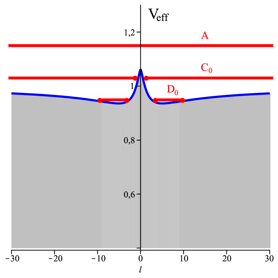
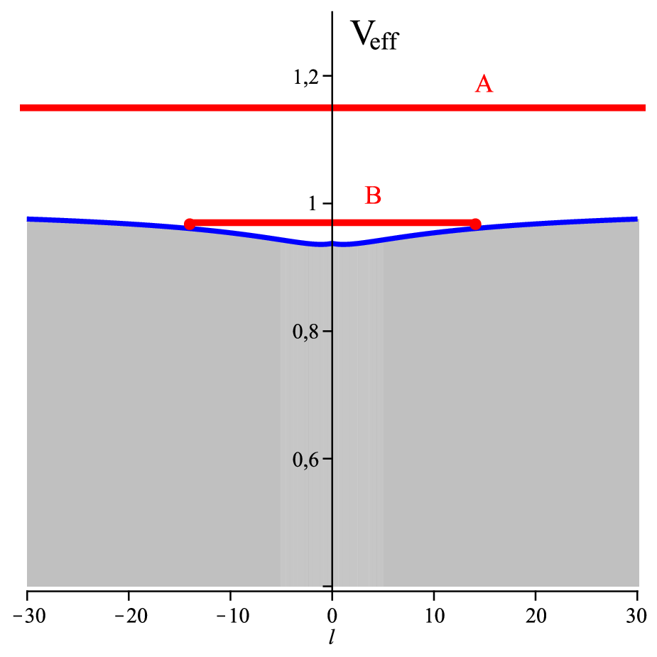
Figure 1 shows examples of the effective potential (14) for massive test particles with $\delta=1$ for different values of $b_{0}$. Here the coordinate $l$ was used. The regions which do not satisfy the condition $E^{2}\geq V_{\rm{eff}}$ are forbidden and colored grey.

The following types of orbits exist in the Schwarzschild-wormhole spacetime for massive test particles:

• Type $A$

  two-world escape orbit TWE which connect two parts of the Universe. These orbits would be ending at the singularity in usual Schwarzschild spacetime.

• Type $B$

  two-world bound orbits TWB when a test particle moves on a bound orbit stretching from one into another part of the Universe. This orbit connects the upper and lower parts of the universe similar to the orbit of type A.

• Type $C$

  this type contains two possible orbits: two-world bound TWB and escape orbits EO. EOs exist in both parts of the Universe. For growing values of the throat parameter $b_{0}$ this type reduces to $C_{0}$ containing only EOs. See Fig.1(b).

• Type $D$

  this type includes two-world bound TWB and bound orbits BO. BOs exist in both parts of the Universe. Here again $D$ reduces to type $D_{0}$ for growing values of the throat parameter $b_{0}$. See Fig.1(b).

For large $b_{0}$-values only orbits of type $B$ and $A$ survive (Fig.1(c)). For very large values - only type $A$ is possible.

Figure 1(d) shows a set of potential plots for large $L^{2}=9$, when no planetary bound orbits are possible (also in the Schwarzschild black hole spacetime), and different values of the throat parameter $b_{0}$.

Geodesics of massive test particles described by the solution (9) are shown in Fig.2. In this Figure, the two-world bound TWB orbit 2(a) and the bound orbit BO 2(b) correspond to type $D$. The two-world bound TWB orbit 2(c) and the escape orbit EO 2(d) are of type $C$, and the two-world-escape orbits TWE 2(e) and 2(f) are of type $A$. The orbits are embedded into the three-dimensional space with the coordinates $(x,y,z)$, where $x=r\cos(\varphi)$, $y=r\sin(\varphi)$, and $r$ and $z$ are given by (9) and (12) correspondingly.

We start with the Kerr metric in Boyer–Lindquist coordinates [54]

where $\Delta=r^{2}+a^{2}-r$ and $\rho^{2}=r^{2}+a^{2}\cos^{2}\vartheta$. The radial coordinate $r$ and the rotation parameter $a$ are normalized to the mass parameter $2M$ and are dimensionless.

The Lagrangian for a free test particle following a geodesic in the equatorial plane $\vartheta=\frac{\pi}{2}$ yields

where $\delta=0$ for null geodesics and $\delta=1$ for time-like geodesics, and $\dot{x^{\alpha}}$ is the derivative with respect to the affine parameter $\lambda$.

The conserved and dimensionless energy $E=-\frac{\partial\mathcal{L}}{\partial\dot{t}}$ and angular momentum $L=\frac{\partial\mathcal{L}}{\partial\dot{\varphi}}$ of a free test particle are

Solving the equations (17) and (18) with respect to $\dot{t}$ and $\dot{\varphi}$ and substituting them into the Lagrangian (16) we obtain the differential equations describing the motion of a free test particle in the equatorial plane [54, 55]

Here $\gamma$ is a new affine parameter related to $\lambda$ by $d\gamma=r^{-2}d\lambda$.

The ergosphere, defined by the condition $g_{tt}=0$, is located at $r=1$ for the equatorial plane. The condition $g_{rr}\rightarrow\infty$ corresponding to the vanishing of $\Delta$ defines the two horizons of the Kerr spacetime: $h_{1,2}=(1\mp\sqrt{1-4a^{2}})/2$.

In the following we will solve the diffential equations (17) and (18) using the theory of elliptic functions [60].

The throat of the Kerr wormhole lies behind the horizons: $b_{0}>h_{2}$. Following [17] we assume that the thin-shell Kerr-wormhole with the throat parameter $b_{0}$ does not depend on the proper time and, thus, is constant. Similar to the Sec. II.2 we use the surgery method to construct the thin-shell Kerr-wormhole. Namely, we cut the Kerr spacetime at some $b_{0}>h_{2}$ and glue two copies of the manifold $M_{1,2}=(t,r,\vartheta,\varphi|r\geq b_{0})$ onto each other. Identifying the boundaries of these copies we get a new geodesically complete manifold with two regions connected by a wormhole with the throat characterized by the parameter $b_{0}$. The new coordinate $|l|=|r-b_{0}|$ running from $-\infty$ to $\infty$ and vanishing at the throat is a practical coordinate to portray the effective potential (32) (see Fig.4 and Fig.5 in the Sec.III.3).

To understand the Kerr-wormhole topology for the equatorial plane motion described by the functions (23) and (27), consider the two dimensional hypersurface $(t=const,\vartheta=\pi/2)$ described by the geometry:

where $R^{2}=r^{2}+a^{2}+\frac{a^{2}}{r}$ and $\Delta=r^{2}+a^{2}-r$. This two-dimensional hypersurface can be embedded into the Euclidean space given by

in the cylindrical coordinates $(r,\varphi,z)$.

Comparing the coefficients of $dr^{2}$ in (28) and (29) we find that the shape of the embedding diagram in the Euclidean space is given by the integral

and is visualized in Fig.6 in coordinates $(x,y,z)$, where $x=r\cos(\varphi)$ and $y=r\sin(\varphi)$ (to the discussion of the orbits we will come in the next section). The integral in (30) is calculated numerically. For the embedding diagram we choose the initial value of $r$ to be $b_{0}$ and $\varphi\in[0,2\pi]$.

We introduce the effective potential via equation (19)

Thus, the effective potential in the Kerr spacetime is given by [54, 55, 56]

The intersections of the function $E$ and $V_{\rm{eff}}$ specify the turning points of the motion.

The graphical representation of the effective potential (32) is shown in Fig.4, where the coordinate $|l|=|r-b_{0}|$ is used. The regions which do not satisfy the condition $E\geq V^{+}_{\rm{eff}}$ and $E\leq V^{-}_{\rm{eff}}$ are forbidden and colored grey.

The orbit types in the thin-shell Kerr-wormhole are very similar to those in the thin-shell Schwarzschild-wormhole. Namely,

• Type $A$

  two-world escape orbit TWE which connects two regions of the Universe. In the Kerr black hole spacetime this orbit would continue into the negative radial coordinate region.

• Type $B$

  two-world bound orbits TWB. A test particle moves on a bound orbit which is partly located in the lower (respectively, upper) Universe, so that, a particle flies through the throat.

• Type $C$

  here two-world bound TWB and escape orbits EO are possible. EOs exist in both parts of the Universe. For growing values of the throat parameter $b_{0}$ this type reduces to $C_{0}$ containing only EOs. See Fig.4(c).

• Type $D$

  two-world bound TWB and bound orbits BO are possible. BOs exist in both parts of the Universe. For growing values of the throat parameter $b_{0}$ the type $D$ reduces to $D_{0}$ containing only BOs (see Fig.4(c)).

For a further growing throat parameter $b_{0}$, TWB (type $B$) and TWE (type $A$) exist (see Fig.4(d)). For larger $b_{0}$ only the TWE (type $A$) orbits remain. In Fig.5 we make $L$ (in 5(a)) and $a$ (in 5(b)) change. In the first case, similar to the Kerr black hole spacetime, for large angular momenta of a test particle no planetary bound orbits exist. In the second case the form of the effective potential transforms when $a$ tends to the critical value $a_{\rm crit}=0.5$ when the horizons in the Kerr black-hole spacetime merge.

We illustrate these orbit types in Figs.6 and 7. Fig. 7, plotted for opposite signs of the rotation parameter of the wormhole and the angular momentum of a test particle, also shows the influence of the ergosphere. It can be recognized in the directional change taking place shortly before the black circle is approached, which symbolizes the wormhole throat in the pictures 7(a) for the TWB and 7(d) for the TWE orbit. The ergoregion in the Kerr wormhole spacetime surrounds the throat. The corresponding orbits are shown in 7(b) and 7(e). The trajectories are embedded into the three-dimensional space with the coordinates $(x,y,z)$, where $x=r\cos(\varphi)$, $y=r\sin(\varphi)$, and $r$, $\varphi$ and $z$ are given by (23), (27) and (30) correspondingly.

References

- [1] A. Einstein, N. Rosen, Phys. Rev. 48, 73 (1935)
- [2] J. A. Wheeler, Geometrodynamics (Academic Press, New York, 1962)
- [3] R. W. Fuller, J. A. Wheeler, Phys. Rev. 128, 919 (1962)
- [4] M. S. Morris, K. S. Thorne, Wormholes in spacetime and their use for interstellar travel: a tool for teaching general relativity, Am. j. Phys. 56, 395 (1988)
- [5] M. Visser, Traversable wormholes: some simple exmaples, Phys. Rev. D 39, 3182 (1989)
- [6] M. Visser, Traversable wormholes from surgically modified Schwarzschild spacetimes, Nuclear Physics B 328, 203 (1989)
- [7] E. Poisson, M. Visser, Thin-shell wormholes: Linearization stability, Phys. Rev. D 52, 7318 (1989)
- [8] S. Shushkov, Wormholes supported by a phantom energy, Phys. Rev. D 71,043520 (2005)
- [9] F. S. N. Lobo, Phantom energy traversable wormholes, Phys. Rev. D 71,084011 (2005)
- [10] O. B. Zaslavskii, Exactly Solvable Model of a Wormhole Supported by Phantom Energy, Phys. Rev. D, 72, 061303 (2005)
- [11] P. K. F. Kuhfittig, Seeking Exactly Solvable Models of Traversable Wormholes Supported by Phantom Energy, Class. Quantum Grav., 23, 5853 (2006)
- [12] F. Rahaman, M. Kalam, M. Sarkar, K. Gayen, A Theoretical Construction of Wormhole Supported by Phantom Energy, Phys. Lett. B, 633, 161 (2006)
- [13] A. Das, S. Kar, The Ellis wormhole with ‘tachyon matter’, Class. Quantum Grav. 22, 3045 (2005)
- [14] F. S. N. Lobo, Chaplygin traversable wormholes, Phys. Rev. D 73, 064028 (2006)
- [15] E. F. Eiroa, C. Simeone, Stability of Chaplygin gas thin-shell wormholes, Phys. Rev. D 76, 024021 (2007)
- [16] E. F. Eiroa, Thin-shell wormholes with a generalized Chaplygin gas, Phys. Rev. D 80, 044033 (2009)
- [17] P. E. Kashgarin, S. V. Sushkov, Rotating Thin-Shell Wormhole from Glued Kerr Spacetimes, Gravitationa and Cosmology 17, 119 (2011)
- [18] P. K. F. Kuhfittig, Can a wormhole supported by only small amounts of exotic matter really be traversable?, Phys. Rev. D, 68, 067502 (2003)
- [19] P. K. F. Kuhfittig, Wormholes supported by a combination of normal and quintessential matter in Einstein and Einstein-Maxwell gravity, Journal of Modern Physics 4, 30, 2013
- [20] E. F. Eiroa, M. G. Richarte, C. Simeone, Thin-shell wormholes in Brans-Dicke gravity, Phys.Lett. A373, 1-4 (2008); Erratum-ibid A373, 2399-2400 (2009)
- [21] E. F. Eiroa , G. E. Romero, Linearized stability of charged thin shell wormholes, Gen. Rel. Grav. 36, 651 (2004)
- [22] E. F. Eiroa, Stability of thin-shell wormholes with spherical symmetry, Phys. Rev. D 78, 024018 (2008)
- [23] F. S. N. Lobo, P. Crawford, Linearized stability analysis of thin-shell wormholes with a cosmological constant , Class. Quantum Grav. 21, 391 (2004)
- [24] F. S. N. Lobo, P. Crawford, Stability analysis of dynamic thin shells, Class. Quantum Grav. 22, 1 (2005)
- [25] N. Montelongo Garcia, F. S. N. Lobo, M. Visser, Generic spherically symmetric dynamic thin-shell traversable wormholes in standard general relativity, Phys. Rev. D 86, 044026 (2012)
- [26] M. Visser, Wormholes: from Einstein to Hawking (American Institute of physics, Woodbury, 1995)
- [27] F. S. N. Lobo, Exotic solutions in General Relativity: Traversable wormholes and “warp drive” spacetimes, arXiv:0710.4474, to appear in an edited collection ‘Classical and Quantum Gravity Research Progress’, Nova Science Publishers
- [28] F. Rahaman, P.K.F. Kuhfittig, S. Ray, S. Islam, Searching for higher-dimensional wormholes with noncommutative geometry, Phys. Rev. D 86, 106010 (2012)
- [29] P.K.F. Kuhfittig, On the Stability of Thin-Shell Wormholes in Noncommutative Geometry, Advances in High Energy Physics, 2012 Article ID 462493 (2012)
- [30] E. F. Eiroa, C. Simeone, Thin-shell wormholes in dilaton gravity, Phys. Rev. D 71, 127501 (2005)
- [31] M, Thibeault, C. Simeone, E. F. Eiroa, Thin-shell wormholes in Einstein-Maxwell theory with a Gauss-Bonnet term, Gen. Rel. Grav. 38, 1593 (2006)
- [32] M. G. Richarte, Wormholes and solitonic shells in five-dimensional DGP theory, Phys.Rev.D 82, 044021 (2010)
- [33] M. G. Richarte, C. Simeone, Thin-shell wormholes supported by ordinary matter in Einstein–Gauss–Bonnet gravity, Phys.Rev.D 76, 087502 (2007); Erratum-ibid Phys.Rev.D 77, 089903 (2008)
- [34] P. Kanti, B. Kleihaus, J. Kunz, Wormholes in Dilatonic Einstein-Gauss-Bonnet Theory, Phys. Rev. Lett. 107, 271101 (2011)
- [35] P. Kanti, B. Kleihaus, J. Kunz, Stable Lorentzian wormholes in dilatonic Einstein-Gauss-Bonnet theory, Phys. Rev. D 85, 044007 (2012)
- [36] V. Dzhunushaliev, V. Folomeev, B. Kleihaus, J. Kunz, A star harbouring a wormhole at its core, JCAP 04, 031 (2011); DOI: 10.1088/1475-7516/2011/04/031
- [37] V. Dzhunushaliev, V. Folomeev, B. Kleihaus, J. Kunz, Mixed neutron-star-plus-wormhole systems: Equilibrium configurations, Phys. Rev. D 85, 124028 (2012)
- [38] V. Dzhunushaliev, V. Folomeev, B. Kleihaus, J. Kunz, Mixed neutron-star-plus-wormhole systems: Linear stabil ity analysis, arXiv:1302.5217 [gr-qc] (2013)
- [39] F. Schein, P. C. Aichelburg, Traversable wormholes in geometries of charged shells, Phys. Rev. Lett 77, 4130 (1996)
- [40] T. Müller, Exact geometric optics in a Morris-Thorne wormhole spacetime, Phys. Rev. D 77, 044043 (2008)
- [41] O. Sarbach, T. Zannias, The propagation of particles and fields in wormhole geometries, AIP Conf.Proc. 1473 223 (2012); arXiv:1204.3977 [gr-qc]
- [42] A. Abdujabbarov, B. Ahmedov, Electromagnetic fields and charged particle motion around magnetized wormholes, Astrophys Space Sci 321, 225 (2009)
- [43] E. Teo, Rotating traversable wormholes, Phys. Rev. D 58, 024014 (1998)
- [44] P. K. F. Kuhfittig, Axially symmetric rotating traversable wormholes, Phys. Rev. D 67 064015 (2003)
- [45] P. E. Kashargin, S.V. Sushkov, Slowly rotating scalar field wormholes: The second order approximation, Phys. Rev. D 78, 064071 (2008)
- [46] T. Matos, D. Núñez, Rotating scalar field wormhole, Class. Quantum Grav. 23, 4485 (2006)
- [47] M. Jamil, Can a wormhole generate electromagnetic field?, Int. J. Theor. Phys. 49, 1549 (2010)
- [48] T. Matos, Class of Einstein–Maxwell phantom fields: rotating and magnetized wormholes, Gen. Relativ. Gravit., DOI 10.1007/s10714-010-0976-6 (2010)
- [49] M. S. Morris, K. S. Thorne, U. Yurtsever, Wormholes, Time Machines, and the Weak Energy Condition, Phys. Rev. Lett. 61, 1446 (1988)
- [50] V. P. Frolov, I. D. Novikov, Physical effects in wormholes and time machines, Phys. Rev. D 42, 1057 (1990)
- [51] V. P. Frolov, Vacuum polarization in a locally static multiply connected spacetime and a time-machine problem, Phys. Rev. D 43, 3878 (1991)
- [52] S. W. Kim, K. S. Thorne, Do vacuum Fluctuations prevent the creation of closed timelike curves?, Phys. Rev. D 43, 3929 (1991)
- [53] S. W. Hawking, Chronology protection conjecture, Phys. Rev. D 46, 603 (1992)
- [54] S. Chandrasekhar, The Mathematical Theory of Black Holes (Oxford University Press, Oxford, 1983).
- [55] B. O’Neil, The Geometry of Kerr Black Holes (A.K. Peters, Wellesley, MA, 1995).
- [56] D. Pugliese, H. Quevedo, R. Ruffini, Equatorial circular motion in Kerr spacetime, Phys. Rev. D 84, 044030 (2011)
- [57] J. B. Hartle, Gravity, (Addison Wesley, San Francisco, 2003).
- [58] B. F. Schutz, A first course in general relativity, (Cambridge University Press, Cambridge, UK, 1985).
- [59] S. L. Shapiro, S. A. Teukolsky Black holes, white dwarfs, and neutron stars, (John Wiley & Sons, New York, Chichester, Brisbane, Toronto, Singapore, 1983).
- [60] A. I. Markushevich, Theory of functions of a complex variable, Vol. III, Prentice-Hall, Inc., Englewood Cliffs, N.J. (1967).
- [61] S. Grunau, V. Kagramanova, Geodesics of electrically and magnetically charged test particles in the Reissner-Nordström spacetime: analytical solutions, Phys. Rev. D 83, 044009 (2011).
- [62] V. Kagramanova, S. Reimers, Analytic treatment of geodesics in five-dimensional Myers-Perry spacetimes, Phys. Rev. D 86, 084029 (2012)
- [63] V. Kagramanova, J. Kunz, E. Hackmann and C. Lämmerzahl, Analytic treatment of complete and incomplete geodesics in Taub-NUT spacetimes, Phys. Rev. D 81, 124044 (2010)
- [64] V. Kagramanova, E. Smolarek, Dynamics of test particles in thin-shell wormhole spacetimes II, under preparation (2013)