Non-linear noise excitation
and intermittency under high disorderThanks: Research supported in part by the NSF grant DMS-1006903

Davar Khoshnevisan Affiliation: University of Utah Kunwoo Kim Affiliation: University of Utah

Last update: March 3, 2013

Abstract

Consider the semilinear heat equation $\partial_{t}u=\partial^{2}_{x}u+\lambda\sigma(u)\xi$ on the interval $[0\,,1]$ with Dirichlet zero boundary condition and a nice non-random initial function, where the forcing $\xi$ is space-time white noise and $\lambda>0$ denotes the level of the noise. We show that, when the solution is intermittent [that is, when $\inf_{z}|\sigma(z)/z|>0$ ], the expected $L^{2}$ -energy of the solution grows at least as $\exp\{c\lambda^{2}\}$ and at most as $\exp\{c\lambda^{4}\}$ as $\lambda\to\infty$ . In the case that the Dirichlet boundary condition is replaced by a Neumann boundary condition, we prove that the $L^{2}$ -energy of the solution is in fact of sharp exponential order $\exp\{c\lambda^{4}\}$ . We show also that, for a large family of one-dimensional randomly-forced wave equations, the energy of the solution grows as $\exp\{c\lambda\}$ as $\lambda\to\infty$ . Thus, we observe the surprising result that the stochastic wave equation is, quite typically, significantly less noise-excitable than its parabolic counterparts.

Keywords: The stochastic heat equation; the stochastic wave equation; intermittency; non-linear noise excitation.

AMS 2000 subject classification: Primary 60H15, 60H25; Secondary 35R60, 60K37, 60J30, 60B15.

1 Introduction

The principal aim of this paper is to study the non-linear effect of noise in stochastic partial differential equations whose solutions are “intermittent.” Our analysis is motivated in part by a series of computer simulations that we would like to present first.

Consider the following stochastic heat equation on the interval $[0\,,1]$ with homogeneous Dirichlet boundary conditions:

\left[\begin{split}&\frac{\partial}{\partial t}u_{t}(x)=\frac{1}{2}\frac{\partial^{2}}{\partial x^{2}}u_{t}(x)+\lambda u_{t}(x)\xi&\text{for $0<x<1$ and $t>0$},\\ &u_{t}(0)=u_{t}(1)=0&\text{for $t>0$},\\ &u_{0}(x)=\sin(\pi x)&\text{for $0<x<1$}.\end{split}\right.

(1.1)

Here, $\xi$ denotes space-time white noise on $(0\,,\infty)\times[0\,,1]$ , and $\lambda>0$ is an arbitrary parameter that is known as the level of the noise.

The stochastic partial differential equation (1.1) and its variations are sometimes referred to as parabolic Anderson models. Those are a family of noise-perturbed partial differential equations that arise in a diverse number of scientific disciplines. For a representative sample see Balázs et al [1], Bertini and Cancrini [2], Carmona and Molchanov [8], Corwin [9], Cranston and Molchanov [10], Cranston, Mountford, and Shiga [11, 12], Gärtner and König [17], den Hollander [15], Kardar [20], Kardar et al [21], Majda [23], Molchanov [24], and Zeldovich et al [28], together with their substantial bibliographies.

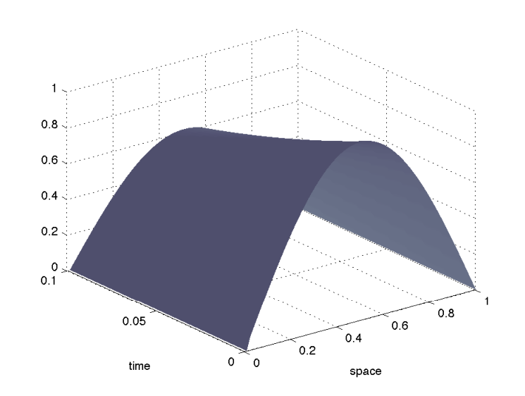
Since the initial function is the principle eigenfunction of the Dirichlet Laplacian on $[0\,,1]$ , it is easy to see that the solution is exactly $u_{t}(x)=\sin(\pi x)\exp\{-\pi^{2}t/2\}$ when $\lambda=0$ ; this is the noise-free case, and a numerical solution is shown is in Figure 1.

Figures 2, 3, and 4 contain simulations of the solution to (1.1) for respective noise levels $\lambda=0.1$ , $\lambda=2$ , and $\lambda=5$ .

Refer to caption — Figure 1: No noise ( $\lambda=0.0$ , maximum height $=1.00$ )

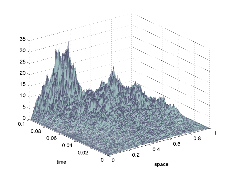
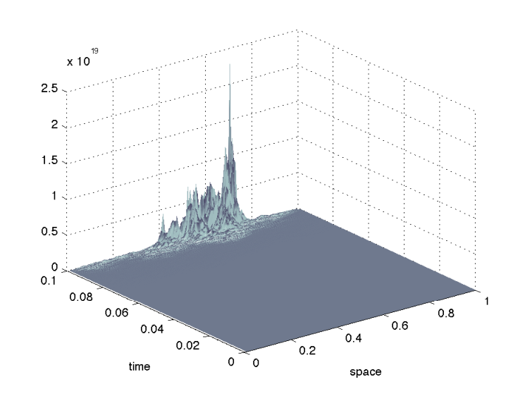
One might notice that, as $\lambda$ increases, the simulated solution rapidly develops tall peaks that are distributed over relatively-small “islands.” This general phenomenon is called intermittency; see Gibbons and Titi [18] for a modern general discussion of intermittency and its ramifications, as well as connections to other important topics [in particular, to turbulence]. Our discussion is motivated in part by the discussion in Blümich [3] on the quite-different topic of NMR spectroscopy.

Presently, we study non-linear noise-excitation phenomena for stochastic partial differential equations that include the parabolic Anderson model (1.1) as a principle example. Namely, let us choose and fix a length scale $L>0$ , and then consider the stochastic partial differential equation,

\left[\begin{split}&\frac{\partial}{\partial t}u_{t}(x)=\frac{\partial^{2}}{\partial x^{2}}u_{t}(x)+\lambda\sigma(u_{t}(x))\xi&\text{for $0<x<L$ and $t>0$},\\ &u_{t}(0)=u_{t}(L)=0&\text{for $t>0$},\end{split}\right.

(1.2)

where $\sigma:\mathbf{R}\to\mathbf{R}$ is a Lipschitz-continuous function, $\xi$ denotes space-time white noise as before, and the initial function $u_{0}:[0\,,L]\to\mathbf{R}_{+}$ is a non-random bounded continuous function that is non-negative everywhere on $[0\,,L]$ and strictly positive on a set of positive Lebesgue measure in $(0\,,L)$ . For the sake of simplicity, we assume further that $\sigma(0)=0$ , though some of our work remains valid when $\sigma(0)\neq 0$ as well.

It is well known that the stochastic heat equation (1.2) has an a.s.-unique continuous solution that has the property that

\sup_{x\in[0,L]}\sup_{t\in[0,T]}\mathrm{E}\left(|u_{t}(x)|^{k}\right)<\infty\qquad\text{for all $T>0$ and $k\in[2\,,\infty)$}.

(1.3)

We will be interested in the effect of the level $\lambda$ of the noise on the [expected] energy $\mathscr{E}_{t}(\lambda)$ of the solution at time $t$ ; the latter quantity is defined as

\mathscr{E}_{t}(\lambda):=\sqrt{\mathrm{E}\left(\|u_{t}\|_{L^{2}[0,L]}^{2}\right)}\qquad(t>0).

(1.4)

Throughout, we use the following notation:

\ell_{\sigma}:=\inf_{z\in\mathbf{R}\setminus\{0\}}\left|\frac{\sigma(z)}{z}\right|,\qquad\text{\rm L}_{\sigma}:=\sup_{z\in\mathbf{R}\setminus\{0\}}\left|\frac{\sigma(z)}{z}\right|.

(1.5)

Clearly, $0\leqslant\ell_{\sigma}\leqslant\text{\rm L}_{\sigma}$ . Moreover, $\text{\rm L}_{\sigma}<\infty$ because $\sigma$ is Lipschitz continuous.

The following two theorems contain quantitative descriptions of the non-linear noise excitability of (1.2). These are the main findings of this paper.

Theorem 1.1.

For all $t>0$ ,

\frac{\ell_{\sigma}^{2}t}{2}\leqslant\liminf_{\lambda\to\infty}\frac{1}{\lambda^{2}}\log\mathscr{E}_{t}(\lambda),\quad\limsup_{\lambda\to\infty}\frac{1}{\lambda^{4}}\log\mathscr{E}_{t}(\lambda)\leqslant 8\text{\rm L}_{\sigma}^{4}t.

(1.6)

In a companion paper [22] we show that $\exp\{c\lambda^{4}\}$ is a typical lower bound for the energy of a large number of intermittent complex systems. In particular, the energy of the solution for the stochastic heat equation on $[0\,,L]$ with a periodic boundary condition is shown to be of sharp exponential order $\exp\{c\lambda^{4}\}$ . The following theorem says that we can get the same kind of result when we replace a Dirichlet with a Neumann boundary condition, provided additionally that the initial profile remains bounded uniformly away from zero.

Theorem 1.2.

Suppose that we replace the Dirichlet boundary condition in (1.2) by a Neumann boundary condition; that is, we suppose that $u$ solves the following stochastic heat equation:

\left[\begin{split}&\frac{\partial}{\partial t}u_{t}(x)=\frac{\partial^{2}}{\partial x^{2}}u_{t}(x)+\lambda\sigma(u_{t}(x))\xi&\text{for $0<x<L$ and $t>0$},\\ &\frac{\partial u_{t}}{\partial x}(0)=\frac{\partial u_{t}}{\partial x}(L)=0&\text{for $t>0$}.\end{split}\right.

(1.7)

If, in addition, we assume that $\inf_{x\in[0,L]}u_{0}(x)>0$ , then for every $t>0$ ,

\frac{\ell_{\sigma}^{4}t}{8\pi{\rm e}}\leqslant\liminf_{\lambda\uparrow\infty}\frac{1}{\lambda^{4}}\log\mathscr{E}_{t}(\lambda)\leqslant\limsup_{\lambda\uparrow\infty}\frac{1}{\lambda^{4}}\log\mathscr{E}_{t}(\lambda)\leqslant\frac{9\text{\rm L}_{\sigma}^{4}t}{16}.

(1.8)

Theorems 1.1 and 1.2 together show that under fairly natural regularity conditions [that include $\ell_{\sigma}>0$ ], the energy behaves roughly as $\exp\{c\lambda^{4}\}$ , which is a fastly-growing function of the level $\lambda$ of the noise. In Section 4 we document the somewhat surprising fact that, by contrast, the stochastic wave equation has typically an energy that grows merely as $\exp\{c\lambda\}$ . In other words, the stochastic wave equation is typically substantially less noise excitable than the stochastic heat equation.

2 Proof of Theorem 1.1

As is customary, we begin by writing the solution to the stochastic heat equation (1.2) in integral form [also known as the mild form],

u_{t}(x)=(P_{t}u_{0})(x)+\lambda\int_{(0,t)\times(0,L)}p_{t-s}(x\,,y)\sigma(u_{s}(y))\,\xi({\rm d}s\,{\rm d}y),

(2.1)

where $\{P_{t}\}_{t\geqslant 0}$ denotes the semigroup of the Dirichlet Laplacian on $[0\,,L]$ and $\{p_{t}\}_{t>0}$ denotes the corresponding heat kernel. That is, in particular, $P_{0}h\equiv h$ for every $h\in L^{\infty}[0\,,L]$ , and

(P_{t}h)(x):=\int_{0}^{L}p_{t}(x\,,y)h(y)\,{\rm d}y\qquad\text{for all $t>0$ and $x\in[0\,,L]$}.

(2.2)

One can expand the heat kernel $p_{t}(x\,,y)$ —the fundamental solution to the Dirichlet Laplacian on $[0\,,L]$ —in terms of the eigenfunctions of the Dirichlet Laplacian as follows:

p_{t}(x\,,y):=\sum_{n=1}^{\infty}\phi_{n}(x)\phi_{n}(y){\rm e}^{-\mu_{n}t};

(2.3)

where

\mu_{n}:=\left(\frac{n\pi}{L}\right)^{2},\quad\phi_{n}(x):=\left(\frac{2}{L}\right)^{1/2}\sin\left(\frac{n\pi x}{L}\right),

(2.4)

for all $n\geqslant 1$ and $0\leqslant x\leqslant L$ . According to the maximum principle: (i) $p_{t}(x\,,y)>0$ for all $t>0$ and $x,y\in(0\,,L)$ ; and (ii) $\int_{0}^{L}p_{t}(x\,,y)\,{\rm d}x<1$ for all $y\in[0\,,L]$ and $t>0$ .

Next we recall, briefly, how to one establishes the existence of a mild solution to (1.2).

Let $u^{(0)}_{t}(x):=u_{0}(x)$ for all $x\in[0\,,L]$ and $t\geqslant 0$ , and then define iteratively, for all $k\geqslant 0$ ,

u^{(k+1)}_{t}(x)=(P_{t}u_{0})(x)+\lambda\int_{(0,t)\times(0,L)}p_{t-s}(x\,,y)\sigma(u^{(k)}_{s}(y))\,\xi({\rm d}s\,{\rm d}y).

(2.5)

Then the method of Walsh [27, Chapter 3]—see Dalang [13]—shows that $\{u^{(n)}\}_{t\geqslant 0}$ is locally uniformly Cauchy in $L^{2}(\mathrm{P})$ in the sense that for all $T>0$ ,

\sum_{k=1}^{\infty}\sup_{x\in[0,L]}\sup_{t\in[0,T]}\sqrt{\mathrm{E}\left(|u^{(k+1)}_{t}(x)-u^{(k)}_{t}(x)|^{2}\right)}<\infty.

(2.6)

It follows fairly easily from this that $u:=\lim_{k\to\infty}u^{(k)}_{t}(x)$ exists in $L^{2}(\mathrm{P})$ and solves (2.5). Moreover, one can deduce that $u$ is unique among all mild solutions that satisfy (1.3)—see Dalang [13] for the details.

Proof of the first bound in Theorem 1.1.

We follow an idea that is classical in the context of PDEs (see Kaplan [19]); in the context of SPDEs, a nontrivial adaptation of this idea was used in Bonder and Groisman [4] in order to compare the solution of an SPDE to the solution to a one-dimensional diffusion in order to describe a certain blow-up phenomenon. In a somewhat loose sense, we follow the same general outline, but need to make a number of modifications along the way.

Recall that $\{\phi_{n}\}_{n=1}^{\infty}$ denote the eigenfunctions of the Dirichlet Laplacian on $[0\,,L]$ and $\{\mu_{n}\}_{n=1}^{\infty}$ are the corresponding eigenvalues. Since $p_{t}(x\,,y)=p_{t}(y\,,x)$ , an appeal to a stochastic Fubini theorem [27, Theorem 2.6, p. 296] implies the following for all $n\geqslant 1$ and $t>0$ : With probability one,

\begin{split}&(u_{t}\,,\phi_{n})\\ &=(u_{0}\,,P_{t}\phi_{n})+\lambda\int_{(0,t)\times(0,L)}(P_{t-s}\phi_{n})(y)\sigma(u_{s}(y))\,\xi({\rm d}s\,{\rm d}y)\\ &={\rm e}^{-\mu_{n}t}(u_{0}\,,\phi_{n})+\lambda\int_{(0,t)\times(0,L)}{\rm e}^{-\mu_{n}(t-s)}\phi_{n}(y)\sigma(u_{s}(y))\,\xi({\rm d}s\,{\rm d}y).\end{split}

(2.7)

Consequently, the Walsh isometry [27, Theorem 2.5, p. 295] shows us that

\begin{split}\mathrm{E}\left[(u_{t}\,,\phi_{n})^{2}\right]&={\rm e}^{-2\mu_{n}t}(u_{0}\,,\phi_{n})^{2}\\ &\quad+\lambda^{2}\int_{0}^{t}{\rm d}s\int_{0}^{L}{\rm d}y\ {\rm e}^{-2\mu_{n}(t-s)}|\phi_{n}(y)|^{2}\mathrm{E}\left(\left|\sigma(u_{s}(y))\right|^{2}\right)\\ &\geqslant{\rm e}^{-2\mu_{n}t}(u_{0}\,,\phi_{n})^{2}\\ &\quad+\lambda^{2}\ell_{\sigma}^{2}\int_{0}^{t}{\rm e}^{-2\mu_{n}(t-s)}\,{\rm d}s\int_{0}^{L}{\rm d}y\ |\phi_{n}(y)|^{2}\mathrm{E}\left(\left|u_{s}(y)\right|^{2}\right).\end{split}

(2.8)

We may apply the Cauchy–Schwarz inequality, together with an appeal to the Fubini theorem, in order to see that

\int_{0}^{L}|\phi_{n}(y)|^{2}\mathrm{E}\left(\left|u_{s}(y)\right|^{2}\right){\rm d}y\geqslant\frac{1}{L}\mathrm{E}\left[(u_{s}\,,\phi_{n})^{2}\right].

(2.9)

Thus we see that, for every fixed $n\geqslant 1$ , the function

F(t):={\rm e}^{2\mu_{n}t}\mathrm{E}\left[(u_{t}\,,\phi_{n})^{2}\right]\qquad(t>0)

(2.10)

satisfies the recursion

F(t)\geqslant(u_{0}\,,\phi_{n})^{2}+\lambda^{2}\ell_{\sigma}^{2}\int_{0}^{t}F(s)\,{\rm d}s\qquad\text{for all $t>0$}.

(2.11)

Thus the Gronwall’s inequality [or just recursion, in this case] shows that

F(t)\geqslant(u_{0}\,,\phi_{n})^{2}\exp\left(\lambda^{2}\ell_{\sigma}^{2}t\right)\qquad(t>0).

(2.12)

Equivalently,

\mathrm{E}\left[(u_{t}\,,\phi_{n})^{2}\right]\geqslant(u_{0}\,,\phi_{n})^{2}\exp\left(\left[\lambda^{2}\ell_{\sigma}^{2}-2\mu_{n}\right]t\right)\qquad(t>0).

(2.13)

Since $\sum_{n=1}^{\infty}(u_{t}\,,\phi_{n})^{2}\leqslant\|u_{t}\|_{L^{2}[0,L]}^{2}$ , thanks to Bessel’s inequality, it remains to prove that the following is strictly positive:

c_{t}:=\sum_{n=1}^{\infty}(u_{0}\,,\phi_{n})^{2}{\rm e}^{-2\mu_{n}t}\qquad\text{for all $t\geqslant 0$}.

(2.14)

But $c_{t}>0$ for all $t\geqslant 0$ simply because we can write $c_{t}=\|P_{t}u_{0}\|_{L^{2}[0,L]}^{2}$ , and this expression is strictly positive, thanks to the maximum principle and the fact that $u_{0}>0$ on a set of positive measure. This concludes the proof of the lower bound on the energy in Theorem 1.1. ∎

Our derivation of the upper bound of Theorem 1.1 requires a few elementary preparatory lemmas.

Lemma 2.1.

For all $\beta,t>0$ :

\sup_{x\in[0,L]}\int_{0}^{t}{\rm e}^{-\beta(t-s)}\,{\rm d}s\int_{0}^{L}{\rm d}y\ [p_{t-s}(x\,,y)]^{2}\leqslant\frac{1}{2\sqrt{\beta}};

(2.15)

and

\int_{0}^{t}{\rm e}^{-\beta(t-s)}\,{\rm d}s\int_{0}^{L}{\rm d}x\int_{0}^{L}{\rm d}y\ [p_{t-s}(x\,,y)]^{2}\leqslant\frac{L}{4\sqrt{\beta}}.

(2.16)

Proof.

Because $|\phi_{n}(x)|\leqslant(2/L)^{1/2}$ for all $x\in[0\,,L]$ and $n\geqslant 1$ ,

	$\displaystyle\int_{0}^{t}{\rm e}^{-\beta(t-s)}\,{\rm d}s\int_{0}^{L}{\rm d}y\ [p_{t-s}(x\,,y)]^{2}$	$\displaystyle=\int_{0}^{t}\sum_{n=1}^{\infty}[\phi_{n}(x)]^{2}{\rm e}^{-2(\beta+\mu_{n})(t-s)}\,{\rm d}s$
		$\displaystyle\leqslant\frac{1}{L}\sum_{n=1}^{\infty}\frac{1}{\beta+(n\pi/L)^{2}}.$		(2.17)

The first bound follows because

\sum_{n=1}^{\infty}\frac{1}{\beta+(n\pi/L)^{2}}\leqslant\int_{0}^{\infty}\frac{{\rm d}x}{\beta+(x\pi/L)^{2}}=\frac{L}{2\sqrt{\beta}},

(2.18)

for all $\beta>0$ . In order to obtain the second bound, we integrate (2.17) $[{\rm d}x]$ , using the fact that $\|\phi_{n}\|_{L^{2}[0,L]}=1$ . ∎

We are now ready to establish the energy upper bound in Theorem 1.1.

Proof of the second bound in Theorem 1.1.

We appeal to the nonlinear renewal-theoretic technique of Foondun and Khoshnevisan [16] in order to establish the following a priori estimate: For every $\delta\in(0\,,1)$ ,

\mathrm{E}\left(|u_{t}(x)|^{m}\right)\leqslant\delta^{-m/2}\|u_{0}\|_{L^{\infty}[0,L]}^{m}\exp\left(2tm^{3}\left(\frac{\lambda\text{\rm L}_{\sigma}}{1-\delta}\right)^{4}\right),

(2.19)

valid uniformly for all $m\in[2\,,\infty)$ , $x\in[0\,,L]$ , and $t\geqslant 0$ . Once this is established, then we set $m=2$ in (2.19), and then integrate $[{\rm d}x]$ , in order to deduce the upper bound of the theorem.

Since $\text{\rm L}_{\sigma}<\infty$ and $\sigma(0)=0$ , it follows that

|\sigma(z)|^{2}\leqslant\text{\rm L}_{\sigma}^{2}|z|^{2}\qquad\text{for all $z\in[0\,,L]$}.

(2.20)

Recall that $u^{(k)}$ denotes the $k$ th-stage Picard iteration approximation to $u$ . According to the Burkholder–Davis–Gundy inequality (see Burkholder [5], Burkholder et al [6], and Burkholder and Gundy [7]; see also Foondun and Khoshnevisan [16] for an explanation of these particular constants),

\left\|\int_{(0,t)\times(0,L)}Z_{s}(y)\,\xi({\rm d}s\,{\rm d}y)\right\|_{m}^{2}\leqslant 4m\int_{0}^{t}{\rm d}s\int_{0}^{L}{\rm d}y\ \left\|Z_{s}(y)\right\|_{m}^{2},

(2.21)

for all predictable random fields $Z$ , all $t>0$ , and $m\in[2\,,\infty)$ , where $\|Q\|_{m}:=\{\mathrm{E}(|Q|^{m})\}^{1/m}$ for all random variables $Q$ . Therefore, we can deduce from (2.5) that

\begin{split}&\left\|u^{(k+1)}_{t}(x)\right\|_{m}\\ &\leqslant|(P_{t}u_{0})(x)|+\lambda\sqrt{4m\int_{0}^{t}{\rm d}s\int_{0}^{L}{\rm d}y\ [p_{t-s}(x\,,y)]^{2}\left\|\sigma(u^{(k)}_{s}(y))\right\|_{m}^{2}}\\ &\leqslant\|u_{0}\|_{L^{\infty}[0,L]}+\lambda\sqrt{4m\text{\rm L}_{\sigma}^{2}\int_{0}^{t}{\rm d}s\int_{0}^{L}{\rm d}y\ [p_{t-s}(x\,,y)]^{2}\left\|u^{(k)}_{s}(y)\right\|_{m}^{2}}.\end{split}

(2.22)

Define

N_{k}(\beta):=\sup_{t\geqslant 0}\sup_{x\in[0,L]}\left({\rm e}^{-\beta t}\left\|u_{t}^{(k)}(x)\right\|_{m}^{2}\right)^{1/2}\qquad(k\geqslant 0,\,\beta>0).

(2.23)

The preceding and Lemma 2.1 together show that

\int_{0}^{t}{\rm d}s\int_{0}^{L}{\rm d}y\ [p_{t-s}(x\,,y)]^{2}\left\|u^{(k)}_{s}(y)\right\|_{m}^{2}\leqslant\left[N_{k}(\beta)\right]^{2}\frac{{\rm e}^{\beta t}}{2\sqrt{\beta}}.

(2.24)

Therefore, we combine our efforts in order to deduce the bound

\left\|u^{(k+1)}_{t}(x)\right\|_{m}\leqslant\|u_{0}\|_{L^{\infty}[0,L]}+\sqrt{2m}\,\lambda\text{\rm L}_{\sigma}{\rm e}^{\beta t/2}\beta^{-1/4}N_{k}(\beta).

(2.25)

Since the right-hand side is independent of $x\in[0\,,L]$ and depends on $t$ only through the term $\exp(\beta t/2)$ , we can divide both sides by $\exp(\beta t/2)$ and optimize over $t$ and $x$ in order to deduce the recursive inequality,

N_{k+1}(\beta)\leqslant\|u_{0}\|_{L^{\infty}[0,L]}+\frac{\lambda\text{\rm L}_{\sigma}\sqrt{2m}}{\beta^{1/4}}N_{k}(\beta).

(2.26)

So far, $\beta$ was an auxiliary positive parameter. We now fix it at the value

\beta_{*}:=\frac{4m^{2}(\lambda\text{\rm L}_{\sigma})^{4}}{(1-\delta)^{4}},

(2.27)

where $\delta\in(0\,,1)$ is arbitrary but fixed. For this particular choice,

N_{k+1}(\beta_{*})\leqslant\|u_{0}\|_{L^{\infty}[0,L]}+(1-\delta)N_{k}(\beta_{*})\qquad(k\geqslant 0).

(2.28)

Because $N_{0}(\beta_{*})=\|u_{0}\|_{L^{\infty}[0,L]}$ , the preceding iteration yields

\sup_{k\geqslant 0}N_{k}(\beta_{*})\leqslant\|u_{0}\|_{L^{\infty}[0,L]}\sum_{j=0}^{\infty}(1-\delta)^{j}=\delta^{-1}\|u_{0}\|_{L^{\infty}[0,L]}.

(2.29)

This and Fatou’s lemma together imply that

\sup_{t\geqslant 0}\sup_{x\in[0,L]}\left({\rm e}^{-\beta_{*}t}\|u_{t}(x)\|_{m}^{2}\right)^{1/2}\leqslant\delta^{-1}\|u_{0}\|_{L^{\infty}[0,L]},

(2.30)

which, in turn, yields (2.19). ∎

3 Proof of Theorem 1.2

Let us now consider the following stochastic heat equation on the interval $[0\,,L]$ , subject to a Neumann boundary condition:

\left[\begin{split}&\frac{\partial}{\partial t}u_{t}(x)=\frac{\partial^{2}}{\partial x^{2}}u_{t}(x)+\lambda\sigma(u_{t}(x))\xi&\text{for $0<x<L$ and $t>0$},\\ &\frac{\partial u_{t}}{\partial x}(0)=\frac{\partial u_{t}}{\partial x}(L)=0&\text{for $t>0$},\end{split}\right.

(3.1)

where $\xi$ denotes space-time white noise as before, and the assumptions on $\sigma$ and $u_{0}(x)$ are also the same as for the Dirichlet problem (1.2). For the sake of simplicity, we assume further that $\sigma(0)=0$ , though some of our work remains valid when $\sigma(0)\neq 0$ as well. We may assume that

\ell_{\sigma}>0.

(3.2)

Otherwise, the more interesting part of Theorem 1.2, that is the lower bound on the energy, has no content. [The proof of the upper bound will not require (3.2).] Also, let us define

\varepsilon:=\inf_{x\in[0,L]}u_{0}(x).

(3.3)

According to the hypotheses of Theorem 1.2, $\varepsilon>0$ .

As we did for the Dirichlet problem, we begin by writing the solution to the stochastic heat equation (3.1) in integral form. Namely, we write

u_{t}(x)=(P_{t}u_{0})(x)+\lambda\int_{(0,t)\times(0,L)}p_{t-s}(x\,,y)\sigma(u_{s}(y))\,\xi({\rm d}s\,{\rm d}y),

(3.4)

where $\{P_{t}\}_{t\geqslant 0}$ denotes the semigroup of the Neumann Laplacian on $[0\,,L]$ and $\{p_{t}\}_{t>0}$ denotes the corresponding heat kernel. That is, $P_{0}h\equiv h$ for every $h\in L^{\infty}[0\,,L]$ , and

(P_{t}h)(x):=\int_{0}^{L}p_{t}(x\,,y)h(y)\,{\rm d}y\qquad\text{for all $t>0$ and $x\in[0\,,L]$}.

(3.5)

It is well known that we can write the heat kernel for $\{P_{t}\}_{t\geqslant 0}$ in the following form:

p_{t}(x\,,y):=\sum_{n=-\infty}^{\infty}\left[\Gamma_{t}(x-y-2nL)+\Gamma_{t}(x+y-2nL)\right],

(3.6)

where $\Gamma$ denotes the fundamental solution to the heat equation in $\mathbf{R}$ ; that is,

\Gamma_{t}(z):=\frac{1}{\sqrt{4\pi t}}\exp\left(-\frac{z^{2}}{4t}\right)\qquad(t>0,z\in\mathbf{R}).

(3.7)

[This requires an application of the method of images.]

The existence and uniqueness of a solution of (3.1) is shown in Walsh [27, Chapter 3]. The following establishes the lower bound of Theorem 1.2.

Proposition 3.1 (An energy inequality).

For all $t>0$ , there exists a finite and positive constant $K$ —independent of $\lambda$ —such that

\mathscr{E}_{t}(\lambda)\geqslant\frac{1}{K}\exp\left(\frac{(\ell_{\sigma}\lambda)^{4}t}{8\pi{\rm e}}\right),

(3.8)

simultaneously for every $\lambda\geqslant 1$ .

Proof of Proposition 3.1.

Owing to (3.6), the Neumann heat kernel is conservative; that is, $\int_{0}^{L}p_{t}(x\,,y)\,{\rm d}y=1$ . Therefore, we apply the Walsh isometry to find that for all fixed $\varepsilon,t>0$ and $x\in[0\,,L]$ ,

	$\displaystyle\mathrm{E}\left(\left\|u_{t}(x)\right\|^{2}\right)$	$\displaystyle\geqslant\varepsilon^{2}+\lambda^{2}\int_{0}^{t}{\rm d}s\int_{0}^{L}{\rm d}y\ [p_{t-s}(x\,,y)]^{2}\mathrm{E}\left(\left\|\sigma(u_{s}(y))\right\|^{2}\right)$
		$\displaystyle\geqslant\varepsilon^{2}+(\lambda\ell_{\sigma})^{2}\int_{0}^{t}{\rm d}s\int_{0}^{L}{\rm d}y\ [p_{t-s}(x\,,y)]^{2}\mathrm{E}\left(\left\|u_{s}(y)\right\|^{2}\right).$

The preceding is a recursive, nonlinear renewal-type, inequality for the function $(t\,,x)\mapsto\mathrm{E}(|u_{t}(x)|^{2})$ . Even though this renewal inequation is the lower bound’s counterpart to (4.11), we cannot solve this inequation using the renewal-theoretic ideas of Foondun and Khoshnevisan [16]. The reason for this is that the method of [16] works for large values of the time variable $t$ ; whereas here we have $t$ fixed, but $\lambda$ large. Instead, we appeal to old ideas of localization of multiple integrals [i.e., classical large deviations] that are probably due to P.-S. Laplace, though we could not find explicit references. Namely, we expand the self-referential inequality (4.17) and observe that most of the contribution to the resulting multiple integrals occur in a small portion of the space of integration.

Now we carry out our program by first expanding, to one term, our renewal inequality as follows:

		$\displaystyle\mathrm{E}\left(\left\|u_{t}(x)\right\|^{2}\right)$
		$\displaystyle\geqslant\varepsilon^{2}+\varepsilon^{2}(\lambda\ell_{\sigma})^{2}\int_{0}^{t}{\rm d}s\int_{0}^{L}{\rm d}y\ [p_{t-s}(x\,,y)]^{2}$		(3.9)
		$\displaystyle\quad+(\lambda\ell_{\sigma})^{4}\int_{0}^{t}{\rm d}s\int_{0}^{L}{\rm d}y\ [p_{t-s}(x\,,y)]^{2}\int_{0}^{s}{\rm d}r\int_{0}^{L}{\rm d}z\ [p_{s-r}(y\,,z)]^{2}\mathrm{E}\left(\left\|u_{r}(z)\right\|^{2}\right),$

and proceed. In order to see better what is happening, let us introduce a family of linear operators $\mathcal{P}$ as follows: For all $t>0$ , $x\in[0\,,L]$ , and all Borel-measurable functions $\psi:(0\,,\infty)\times[0\,,L]\to\mathbf{R}_{+}$ ,

(\mathcal{P}\psi)(t\,,x):=\int_{0}^{t}{\rm d}s\int_{0}^{L}{\rm d}y\ [p_{t-s}(x\,,y)]^{2}\psi(s\,,y).

(3.10)

Also define $\mathbf{1}(t\,,x):=1$ for all $t>0$ and $x\in[0\,,L]$ . Then our recursion can be written compactly as follows:

\mathrm{E}\left(\left|u_{t}(x)\right|^{2}\right)\geqslant\varepsilon^{2}\sum_{k=0}^{\infty}(\lambda\ell_{\sigma})^{2k}(\mathcal{P}^{k}\mathbf{1})(t\,,x);

(3.11)

where $\mathcal{P}^{0}:=\mathbf{1}$ and $\mathcal{P}^{k+1}:=\mathcal{P}^{k}\mathcal{P}$ for all $k\geqslant 0$ . We integrate (3.11) $[{\rm d}x]$ in order to obtain the following key lower bound:

\left|\mathscr{E}_{t}(\lambda)\right|^{2}\geqslant\varepsilon^{2}\sum_{k=0}^{\infty}(\lambda\ell_{\sigma})^{2k}\int_{0}^{L}(\mathcal{P}^{k}\mathbf{1})(t\,,x)\,{\rm d}x.

(3.12)

We examine the preceding sum, term by term, using induction.

The first term in the sum is trivial; viz.,

\int_{0}^{L}(\mathcal{P}^{0}\mathbf{1})(t\,,x)\,{\rm d}x=L.

(3.13)

Therefore, let us consider, as a first step, the second term in the sum, which is straight forward:

\int_{0}^{L}(\mathcal{P}^{1}\mathbf{1})(t\,,x)\,{\rm d}x=\int_{0}^{t}{\rm d}s\int_{0}^{L}{\rm d}x\int_{0}^{L}{\rm d}y\ [p_{t-s}(x\,,y)]^{2}:=\Phi(t).

(3.14)

Before we estimate the third term of the infinite sum in (3.12), let us observe that

		$\displaystyle\int_{0}^{L}(\mathcal{P}^{2}\mathbf{1})(t\,,x)\,{\rm d}x$		(3.15)
		$\displaystyle\qquad=\int_{0}^{t}{\rm d}s\int_{0}^{L}{\rm d}x\int_{0}^{L}{\rm d}y\ [p_{t-s}(x\,,y)]^{2}\int_{0}^{s}{\rm d}r\int_{0}^{L}{\rm d}z\ [p_{s-r}(y\,,z)]^{2}.$

Therefore, we can bound that third term, from below, as follows:

		$\displaystyle\int_{0}^{L}(\mathcal{P}^{2}\mathbf{1})(t\,,x)\,{\rm d}x$		(3.16)
		$\displaystyle\qquad\geqslant\int_{t/2}^{t}{\rm d}s\int_{0}^{L}{\rm d}x\int_{0}^{L}{\rm d}y\ [p_{t-s}(x\,,y)]^{2}\int_{0}^{s}{\rm d}r\int_{0}^{L}{\rm d}z\ [p_{s-r}(y\,,z)]^{2}$
		$\displaystyle\qquad\geqslant\int_{t/2}^{t}{\rm d}s\int_{0}^{L}{\rm d}x\int_{0}^{L}{\rm d}y\ [p_{t-s}(x\,,y)]^{2}\int_{s-t/2}^{s}{\rm d}r\int_{0}^{L}{\rm d}z\ [p_{s-r}(y\,,z)]^{2}$
		$\displaystyle\qquad\geqslant\int_{t/2}^{t}{\rm d}s\int_{0}^{L}{\rm d}x\int_{0}^{L}{\rm d}y\ [p_{t-s}(x\,,y)]^{2}\int_{0}^{t/2}{\rm d}r\int_{0}^{L}{\rm d}z\ [p_{r}(y\,,z)]^{2}$
		$\displaystyle\qquad=\int_{0}^{t/2}{\rm d}s\int_{0}^{t/2}{\rm d}r\int_{0}^{L}{\rm d}x\int_{0}^{L}{\rm d}y\ [p_{s}(x\,,y)]^{2}\int_{0}^{L}{\rm d}z\ [p_{r}(y\,,z)]^{2}.$

It is not important that we have a $t/2$ and in the bounds of our integrals on the second line; $t/{\rm e}$ would have worked equally well for us. The key point is that most of the contribution to our multiple integral comes about where $s\approx t$ and $r\approx s$ in the second line.

Now, let us recall that $p_{r}(y\,,z)$ can be thought of as the transition function for Brownian motion in $(0\,,L)$ , reflected upon reaching the boundary $\{0\,,L\}$ [26]. The Markov property of reflected Brownian motion implies the semigroup property of $\{P_{t}\}_{t\geqslant 0}$ and in particular that $\int_{0}^{L}[p_{r}(y\,,z)]^{2}\,{\rm d}z=p_{2r}(y\,,y)$ . And by symmetry, $\int_{0}^{L}[p_{s}(x\,,y)]^{2}\,{\rm d}x=p_{2s}(y\,,y)$ , as well. Consequently, we obtain

\int_{0}^{L}(\mathcal{P}^{2}\mathbf{1})(t\,,x)\,{\rm d}x\geqslant\int_{0}^{L}\left|\int_{0}^{t/2}\ [p_{2s}(y\,,y)]^{2}\,{\rm d}s\right|^{2}\,{\rm d}y.

(3.17)

Once we understand this, we can see how to bound the remaining terms in the infinite sum in (3.12) as well. In fact, induction shows that

\int_{0}^{L}(\mathcal{P}^{k+1}\mathbf{1})(t\,,x)\,{\rm d}x\geqslant\int_{0}^{L}\left|\int_{0}^{t/(k+1)}\ [p_{2s}(y\,,y)]^{2}\,{\rm d}s\right|^{k+1}\,{\rm d}y,

(3.18)

for all $k\geqslant 1$ . Once again we stress that our multiple integrals are bounded from below by a very small portion of the region of integration.

Finally, we apply Jensen’s inequality in order to see that

\int_{0}^{L}(\mathcal{P}^{k+1}\mathbf{1})(t\,,x)\,{\rm d}x\geqslant L^{-k}\left|\int_{0}^{L}{\rm d}y\int_{0}^{t/(k+1)}{\rm d}s\ [p_{2s}(y\,,y)]^{2}\right|^{k+1},

(3.19)

for all $k\geqslant 1$ . Recall (3.14) in order to see that

\int_{0}^{L}(\mathcal{P}^{k}\mathbf{1})(t\,,x)\,{\rm d}x\geqslant L\left[\frac{\Phi(t/k)}{L}\right]^{k},

(3.20)

for all $k\geqslant 1$ and $t>0$ . This and (3.12) together yield

\begin{split}\left|\mathscr{E}_{t}(\lambda)\right|^{2}&\geqslant\varepsilon^{2}L\cdot\sum_{k=1}^{\infty}\left[\frac{(\lambda\ell_{\sigma})^{2}\Phi(t/k)}{L}\right]^{k}.\end{split}

(3.21)

Finally, we estimate the function $\Phi$ from below.

For all $\tau>0$ ,

\begin{split}\Phi(\tau)&=\int_{0}^{\tau}{\rm d}s\int_{0}^{L}{\rm d}x\int_{0}^{L}{\rm d}y\ [p_{s}(x\,,y)]^{2}\\ &=\int_{0}^{\tau}{\rm d}s\int_{0}^{L}{\rm d}x\ p_{2s}(x\,,x).\end{split}

(3.22)

Since $p_{2s}(x\,,x)\geqslant\Gamma_{2s}(0)=(8\pi s)^{-1/2}$ for all $s>0$ —see (3.6)—the preceding yields the pointwise bound

\Phi(\tau)\geqslant\int_{0}^{\tau}\frac{L}{\sqrt{8\pi s}}\,{\rm d}s=L\sqrt{\frac{\tau}{2\pi}}\qquad(\tau>0).

(3.23)

Thus, we obtain the following:

\begin{split}\left|\mathscr{E}_{t}(\lambda)\right|^{2}&\geqslant\varepsilon^{2}L\cdot\sum_{k=1}^{\infty}\left[\frac{(\lambda\ell_{\sigma})^{2}\sqrt{t}}{\sqrt{2\pi k}}\right]^{k}\\ &\geqslant\varepsilon^{2}L\cdot\sum_{j=1}^{\infty}\left[\frac{(\lambda\ell_{\sigma})^{2}\sqrt{t}}{\sqrt{4\pi j}}\right]^{2j}\\ &\geqslant\varepsilon^{2}L\cdot\sum_{j=1}^{\infty}\left[\frac{(\lambda\ell_{\sigma})^{4}t}{4\pi{\rm e}}\right]^{j}\frac{1}{j!},\end{split}

(3.24)

thanks to the elementary bound, $(j/{\rm e})^{j}\leqslant j!$ , valid for all integers $j\geqslant 1$ . The proposition follows from the preceding and the Taylor series expansion of the exponential function. ∎

Before we prove the upper bound in Theorem 1.2, let us state a simple result regarding the Neumann heat kernel.

Lemma 3.2.

For every $\varepsilon>0$ there exists a positive and finite constant $K:=K_{\varepsilon,L}$ such that

\sup_{t\geqslant 0}\sup_{0\leqslant x\leqslant L}\int_{0}^{t}{\rm e}^{-\beta s}p_{2s}(x\,,x)\,{\rm d}s\leqslant\frac{3+\varepsilon}{\sqrt{8\beta}}\qquad\text{for all $\beta\geqslant K$}.

(3.25)

Proof.

In accord with (3.6), for every $s>0$ and $x\in[0\,,L]$ ,

\begin{split}p_{2s}(x\,,x)&=\sum_{n=-\infty}^{\infty}\left[\Gamma_{2s}(2nL)+\Gamma_{2s}(2x-2nL)\right]\\ &\leqslant 3\Gamma_{2s}(0)+2\sum_{n=1}^{\infty}\Gamma_{2s}(2nL)+\sum_{\begin{subarray}{c}n\in\mathbf{Z}:\\ |nL-x|\geqslant 1\end{subarray}}\Gamma_{2s}(2|nL-x|)\\ &\leqslant 3\Gamma_{2s}(0)+C(L)\\ &=\frac{3}{\sqrt{8\pi s}}+C(L),\end{split}

(3.26)

uniformly for all $s>0$ and $x\in[0\,,L]$ , where $C(L)$ is a positive and finite constant that depends only on $L$ . The numerical bound of $3$ [in front of $\Gamma_{2s}(0)$ ] accounts for the fact that, depending on the value of $x$ , there can be at most two choices of $n\in\mathbf{Z}$ such that $|nL-x|<1$ . We integrate the preceding in order to find that

\int_{0}^{\infty}{\rm e}^{-\beta s}p_{2s}(x\,,x)\,{\rm d}s\leqslant\frac{3}{\sqrt{8\beta}}+\frac{C(L)}{\beta},

(3.27)

which has the desired effect. ∎

We need only to prove the upper bound in Theorem 1.2; the corresponding lower bound has already been established.

Proof of the second bound in Theorem 1.2.

According to the Walsh isometry, for all $t>0$

		$\displaystyle\mathrm{E}\left(\|u_{t}(x)\|^{2}\right)$		(3.28)
		$\displaystyle=\|(P_{t}u_{0})(x)\|^{2}+\lambda^{2}\int_{0}^{t}{\rm d}s\int_{0}^{L}{\rm d}y\ [p_{t-s}(x\,,y)]^{2}\mathrm{E}\left(\left\|\sigma(u_{s}(y))\right\|^{2}\right)$
		$\displaystyle\leqslant\\|u_{0}\\|_{L^{\infty}[0,L]}^{2}+(\lambda\text{\rm L}_{\sigma})^{2}\int_{0}^{t}{\rm d}s\int_{0}^{L}{\rm d}y\ [p_{t-s}(x\,,y)]^{2}\mathrm{E}\left(\left\|u_{s}(y)\right\|^{2}\right).$

We solve this inequality by applying the method of Foondun and Khoshnevisan [16]; namely, let us define, for all $\beta>0$ ,

\mathscr{N}(\beta):=\sup_{t\geqslant 0}\sup_{0\leqslant x\leqslant L}\left[{\rm e}^{-\beta t}\mathrm{E}\left(|u_{t}(x)|^{2}\right)\right].

(3.29)

The preceding and Lemma 3.2 together imply that for all $\varepsilon>0$ there exists $K:=K_{\varepsilon,L}$ such that for all $\beta\geqslant K$ ,

	$\displaystyle\mathscr{N}(\beta)$	$\displaystyle\leqslant\\|u_{0}\\|_{L^{\infty}[0,L]}^{2}+\mathscr{N}(\beta)(\lambda\text{\rm L}_{\sigma})^{2}\sup_{t\geqslant 0}\sup_{0\leqslant x\leqslant L}\int_{0}^{t}{\rm e}^{-\beta s}[p_{2s}(x\,,x)]^{2}\,{\rm d}s$
		$\displaystyle\leqslant\\|u_{0}\\|_{L^{\infty}[0,L]}^{2}+\frac{(3+\varepsilon)(\lambda\text{\rm L}_{\sigma})^{2}}{\sqrt{8\beta}}\mathscr{N}(\beta).$		(3.30)

We let $0<\delta<1$ and choose $\beta$ as

\beta^{*}:=\frac{(3+\varepsilon)^{2}(\lambda\text{\rm L}_{\sigma})^{4}}{8(1-\delta)^{2}},

(3.31)

in order to deduce the inequality

\mathscr{N}(\beta^{*})\leqslant\frac{1}{\delta}\|u_{0}\|_{L^{\infty}[0,L]}^{2},

(3.32)

valid as long as $\lambda$ is large enough to ensure that $\beta^{*}\geqslant K$ . In this way we find that

\mathrm{E}\left(|u_{t}(x)|^{2}\right)\leqslant\frac{1}{\delta}\|u_{0}\|_{L^{\infty}[0,L]}^{2}\exp\left(\frac{(3+\varepsilon)^{2}(\lambda\text{\rm L}_{\sigma})^{4}t}{8(1-\delta)^{2}}\right).

(3.33)

We integrate both sides of (3.33) [ ${\rm d}x$ ] in order to obtain the upper bound, after some relabeling. ∎

4 A stochastic wave equation

In this section we consider the non-linear stochastic wave equation

\frac{\partial^{2}}{\partial t^{2}}w_{t}(x)=\frac{\partial^{2}}{\partial x^{2}}w_{t}(x)+\lambda\sigma(w_{t}(x))\xi\qquad\text{for $x\in\mathbf{R}$ and $t>0$},

(4.1)

subject to non-random initial function $w_{0}(x)\equiv 0$ and non-random non-negative initial velocity $v_{0}\in L^{1}(\mathbf{R})\cap L^{2}(\mathbf{R})$ such that $\|v_{0}\|_{L^{2}(\mathbf{R})}>0$ . It is well known (see Dalang [13] for the general theory, as well as Dalang and Mueller [14], for the existence of an $L^{2}$ -valued solution) that there exists a unique continuous solution $w$ to (4.1) that satisfies the moment conditions,

\sup_{t\in[0,T]}\sup_{x\in\mathbf{R}}\mathrm{E}\left(\left|w_{t}(x)\right|^{k}\right)+\sup_{t\in[0,T]}\mathscr{E}_{t}(\lambda)<\infty,

(4.2)

for every $k\in[2\,,\infty)$ and $T>0$ .

The main result of this section are the following bounds on the energy $\mathscr{E}_{t}(\lambda):=\{\mathrm{E}(\|u_{t}\|_{L^{2}(\mathbf{R})}^{2})\}^{1/2}$ of the solution to (4.1).

Theorem 4.1.

For every $t>0$ ,

\frac{\ell_{\sigma}t}{4\sqrt{8}}\leqslant\liminf_{\lambda\to\infty}\frac{1}{\lambda}\log\mathscr{E}_{t}(\lambda)\leqslant\limsup_{\lambda\to\infty}\frac{1}{\lambda}\log\mathscr{E}_{t}(\lambda)\leqslant\frac{\text{\rm L}_{\sigma}t}{\sqrt{8}}.

(4.3)

Define

H(r):=\frac{r}{2}\wedge\frac{r^{2}}{4}\qquad(r>0).

(4.4)

The preceding theorem requires the following elementary real-variable fact.

Lemma 4.2.

Suppose $g$ is a non-negative element of $L^{1}(\mathbf{R})\cap L^{2}(\mathbf{R})$ . Then, there exist positive and finite constants $A_{1}$ and $A_{2}$ —depending only on $\|g\|_{L^{1}(\mathbf{R})}$ and $\|g\|_{L^{2}(\mathbf{R})}$ —such that

A_{1}H(t)\leqslant\int_{-t}^{t}{\rm d}z\int_{-t}^{t}{\rm d}y\ \left(g*\tilde{g}\right)(y-z)\leqslant A_{2}H(t),

(4.5)

for all $t>0$ , where $\tilde{g}(x):=g(-x)$ for all $x\in\mathbf{R}$ .

Proof.

Define $h:=g*\tilde{g}$ for simplicity, and note that: (i) $h\geqslant 0$ ; (ii) $h\in L^{1}(\mathbf{R})\cap L^{2}(\mathbf{R})$ with $\|h\|_{L^{1}(\mathbf{R})}=\|g\|_{L^{1}(\mathbf{R})}^{2}$ and $h(0)=\|g\|_{L^{2}(\mathbf{R})}^{2}.$ Furthermore, since $h(x)$ is maximized at $x=0$ , thanks to well-known facts about continuous, positive-definite functions. Now we put these facts together in order to see that

\begin{split}\int_{-t}^{t}{\rm d}y\int_{-t}^{t}{\rm d}z\ h(y-z)&\leqslant 4h(0)t^{2}\wedge 2t\|h\|_{L^{1}(\mathbf{R})}\\ &\leqslant 16\left(\|g\|_{L^{2}(\mathbf{R})}^{2}\wedge\|g\|_{L^{1}(\mathbf{R})}^{2}\right)H(t).\end{split}

(4.6)

This proves the upper bound [with an explicit $A_{2}$ ].

On the other hand, $\int_{-t}^{t}{\rm d}y\int_{-t}^{t}{\rm d}z\ h(y-z)=(4+o(1))t^{2}h(0)$ as $t\downarrow 0$ and $\int_{-t}^{t}{\rm d}y\int_{-t}^{t}{\rm d}z\ h(y-z)=(2+o(1))t\|h\|_{L^{1}(\mathbf{R})}$ as $t\uparrow\infty$ . The lower bound follows from these observations, since $h$ is non-negative. ∎

Proof of Theorem 4.1.

The solution to the stochastic wave equation (4.1) can be written in mild form as follows:

w_{t}(x)=\tfrac{1}{2}W_{t}(x)+\tfrac{1}{2}\lambda\int_{(0,t)\times\mathbf{R}}\mathbf{1}_{[0,t-s]}(|x-y|)\sigma(w_{s}(y))\,\xi({\rm d}s\,{\rm d}y),

(4.7)

where

W_{t}(x):=\int_{-t}^{t}v_{0}(x-y)\,{\rm d}y.

(4.8)

Therefore, the Walsh isometry for stochastic integrals assures us that

\begin{split}&\mathrm{E}\left(|w_{t}(x)|^{2}\right)\\ &=\tfrac{1}{4}|W_{t}(x)|^{2}+\tfrac{1}{4}\lambda^{2}\int_{0}^{t}{\rm d}s\int_{-\infty}^{\infty}{\rm d}y\ \mathbf{1}_{[0,t-s]}(|x-y|)\mathrm{E}\left(|\sigma(w_{s}(y))|^{2}\right),\end{split}

(4.9)

whence by Fubini’s theorem,

\begin{split}\left|\mathscr{E}_{t}(\lambda)\right|^{2}&=\tfrac{1}{4}\|W_{t}\|_{L^{2}(\mathbf{R})}^{2}+\tfrac{1}{2}\lambda^{2}\int_{0}^{t}(t-s)\,{\rm d}s\int_{-\infty}^{\infty}{\rm d}y\ \mathrm{E}\left(|\sigma(w_{s}(y))|^{2}\right)\\ &\leqslant\tfrac{1}{4}\|W_{t}\|_{L^{2}(\mathbf{R})}^{2}+\tfrac{1}{2}\lambda^{2}\text{\rm L}_{\sigma}^{2}\int_{0}^{t}(t-s)\,{\rm d}s\int_{-\infty}^{\infty}{\rm d}y\ \mathrm{E}\left(|w_{s}(y)|^{2}\right).\end{split}

(4.10)

Since $\|W_{t}\|_{L^{2}(\mathbf{R})}^{2}=\int_{-t}^{t}{\rm d}y\int_{-t}^{t}{\rm d}z\ (v_{0}*\tilde{v}_{0})(y-z)$ , Lemma 4.2 ensures that the squared energy $\left|\mathscr{E}_{t}(\lambda)\right|^{2}$ of the solution to the stochastic wave equation satisfies the renewal inequality,

\left|\mathscr{E}_{t}(\lambda)\right|^{2}\leqslant A_{2}t^{2}\|v_{0}\|_{L^{2}(\mathbf{R})}^{2}+\tfrac{1}{2}\lambda^{2}\text{\rm L}_{\sigma}^{2}\int_{0}^{t}(t-s)\left(\mathscr{E}_{s}(\lambda)\right)^{2}\,{\rm d}s,

(4.11)

for all $t>0$ .

Since

\sup_{t\geqslant 0}\left[t^{2}{\rm e}^{-\beta t}\right]=\frac{4}{({\rm e}\beta)^{2}},

(4.12)

the preceding implies that

\begin{split}\mathscr{F}(\beta)&\leqslant\frac{4A_{2}}{({\rm e}\beta)^{2}}\|v_{0}\|_{L^{2}[0,L]}^{2}+\tfrac{1}{2}\lambda^{2}\text{\rm L}_{\sigma}^{2}\mathscr{F}(\beta)\int_{0}^{t}(t-s){\rm e}^{-\beta(t-s)}\,{\rm d}s\\ &\leqslant\frac{4A_{2}\|v_{0}\|_{L^{2}[0,L]}^{2}}{({\rm e}\beta)^{2}}+\tfrac{1}{2}\lambda^{2}\text{\rm L}_{\sigma}^{2}\mathscr{F}(\beta)\int_{0}^{\infty}s{\rm e}^{-\beta s}\,{\rm d}s\\ &\leqslant\frac{4A_{2}\|v_{0}\|_{L^{2}[0,L]}^{2}}{({\rm e}\beta)^{2}}+\frac{\lambda^{2}\text{\rm L}_{\sigma}^{2}\mathscr{F}(\beta)}{2\beta^{2}}.\end{split}

(4.13)

Let us choose and fix an arbitrary $\delta\in(0,1)$ . We can apply an a priori method in order to show that $\mathscr{E}(\beta_{*})<\infty$ , where

\beta_{*}:=\frac{\lambda\text{\rm L}_{\sigma}}{\sqrt{2(1-\delta)}}.

(4.14)

See the derivation of (2.19); we omit the details. In this way, we can solve (4.13) in order to deduce the following:

\mathscr{F}(\beta_{*})\leqslant\frac{8A_{2}\|v_{0}\|_{L^{2}[0,L]}^{2}}{\delta({\rm e}\lambda\text{\rm L}_{\sigma})^{2}}.

(4.15)

Equivalently,

\left|\mathscr{E}_{t}(\lambda)\right|^{2}\leqslant\frac{8A_{2}\|v_{0}\|_{L^{2}[0,L]}^{2}}{\delta({\rm e}\lambda\text{\rm L}_{\sigma})^{2}}\exp\left(\frac{\lambda\text{\rm L}_{\sigma}t}{\sqrt{2(1-\delta)}}\right).

(4.16)

This readily yields the upper bound of the theorem.

We prove the corresponding lower bound by observing the following counterpart of (4.11), which holds for the same reasons as (4.11) does:

\left|\mathscr{E}_{t}(\lambda)\right|^{2}\geqslant A_{1}H(t)\|v_{0}\|_{L^{2}[0,L]}^{2}+\tfrac{1}{2}\lambda^{2}\ell_{\sigma}^{2}\int_{0}^{t}(t-s)\left|\mathscr{E}_{s}(\lambda)\right|^{2}\,{\rm d}s.

(4.17)

Now we proceed as we did in the proof of Proposition 3.1; we expand our renewal inequation as an inequality in terms of an infinite sum of multiple integrals of increasingly-high powers. And then show that the multiple integrals are large, when $\lambda\gg 1$ , mainly because of the contribution of the integrand in a small region of integration. In this way the remainder of the proof is exactly the same as the derivation of Proposition 3.1. However, as it turns out, one has to be quite careful in order to guess the correct region of integration, as it will be very significantly larger than the one in the proof Proposition 3.1.

With the preceding in mind, we begin by writing

$\displaystyle\left\|\mathscr{E}_{t}(\lambda)\right\|^{2}$	$\displaystyle\geqslant A_{1}H(t)\\|v_{0}\\|_{L^{2}[0,L]}^{2}+\tfrac{1}{2}\lambda^{2}\ell_{\sigma}^{2}\int_{0}^{t}(t-s)\left(\mathscr{E}_{s}(\lambda)\right)^{2}\,{\rm d}s$
	$\displaystyle\geqslant A_{1}H(t)\\|v_{0}\\|_{L^{2}[0,L]}^{2}+\tfrac{1}{2}A_{1}\lambda^{2}\ell_{\sigma}^{2}\\|v_{0}\\|_{L^{2}[0,L]}^{2}\int_{0}^{t}(t-s)H(s)\,{\rm d}s$
	$\displaystyle\hskip 36.135pt+\left(\tfrac{1}{2}\lambda^{2}\ell_{\sigma}^{2}\right)^{2}\int_{0}^{t}{\rm d}s\int_{0}^{s}{\rm d}r\ (t-s)(s-r)\left\|\mathscr{E}_{r}(\lambda)\right\|^{2},$	(4.18)

etc. In this way, we obtain the following generous lower bound,

		$\displaystyle\left\|\mathscr{E}_{t}(\lambda)\right\|^{2}$		(4.19)
		$\displaystyle\geqslant A_{1}\\|v_{0}\\|_{L^{2}[0,L]}^{2}\sum_{n=1}^{\infty}\left(\tfrac{1}{8}\lambda^{2}\ell_{\sigma}^{2}\right)^{n}\int_{t/2}^{t}{\rm d}s_{1}\int_{s_{1}/2}^{s_{1}}{\rm d}s_{2}\cdots\int_{s_{n-1}/2}^{s_{n-1}}{\rm d}s_{n}\ \mathscr{S},$

where $\mathscr{S}:=(t-s_{1})\times(s_{1}-s_{2})\times\cdots\times(s_{n-1}-s_{n})\times H(t),$ over the range of the integral in (4.19). Let us emphasize that the $n$ th term involves an $n$ -fold integral that is integrate on a large part of the original region of integration; this is in sharp contrast with the proof of Proposition 3.1, where the effective region of integration was extremely small for the $n$ th term when $n\gg 1$ . Once the correct region of integration is identified, we can continue the argument in the proof of Proposition 3.1. Namely, we obtain the following bounds, after we appeal to time reversal:

\begin{split}\left|\mathscr{E}_{t}(\lambda)\right|^{2}&\geqslant A_{1}\|v_{0}\|_{L^{2}[0,L]}^{2}H(t)\cdot\sum_{n=1}^{\infty}\left(\tfrac{1}{8}\lambda^{2}\ell_{\sigma}^{2}\right)^{n}\\ &\hskip 72.26999pt\times\int_{0}^{t/2}{\rm d}s_{1}\int_{0}^{s_{1}/2}{\rm d}s_{2}\cdots\int_{0}^{s_{n-1}/2}{\rm d}s_{n}\ \prod_{j=1}^{n}s_{j}.\end{split}

(4.20)

A change of variables and induction together yield

\begin{split}&\int_{0}^{t/2}{\rm d}s_{1}\int_{0}^{s_{1}/2}{\rm d}s_{2}\cdots\int_{0}^{s_{n-1}/2}{\rm d}s_{n}\ \prod_{j=1}^{n}s_{j}\\ &\hskip 57.81621pt=4^{-n}\int_{0}^{t}{\rm d}s_{1}\int_{0}^{s_{1}}{\rm d}s_{2}\cdots\int_{0}^{s_{n-1}}{\rm d}s_{n}\ \prod_{j=1}^{n}s_{j}\\ &\hskip 57.81621pt=\frac{t^{2n}}{4^{n}\cdot(2n)!!},\end{split}

(4.21)

where $(2n)!!:=(2n)\times(2n-2)\times\cdots\times 2$ denotes the usual double factorial of $2n$ . We require only the simple bound $(2n)!!\leqslant(2n)!$ in order to deduce that

\left|\mathscr{E}_{t}(\lambda)\right|^{2}\geqslant A_{1}\|v_{0}\|_{L^{2}[0,L]}^{2}H(t)\cdot\sum_{n=1}^{\infty}\left(\frac{\lambda\ell_{\sigma}t}{2\sqrt{8}}\right)^{2n}\frac{1}{(2n)!}.

(4.22)

Since

\sum_{n=1}^{\infty}\left(\frac{\lambda\ell_{\sigma}t}{2\sqrt{8}}\right)^{2n+1}\frac{1}{(2n+1)!}\leqslant\sum_{n=1}^{\infty}\left(\frac{\lambda\ell_{\sigma}t}{2\sqrt{8}}\right)^{2n}\frac{1}{(2n)!},

(4.23)

for $\lambda\geqslant 2\sqrt{8}/(t\ell_{\sigma})$ . It follows that

\left|\mathscr{E}_{t}(\lambda)\right|^{2}\geqslant\tfrac{1}{2}A_{1}\|v_{0}\|_{L^{2}[0,L]}^{2}H(t)\cdot\sum_{j=2}^{\infty}\left(\frac{\lambda\ell_{\sigma}t}{2\sqrt{8}}\right)^{j}\frac{1}{j!},

(4.24)

whenever $\lambda\geqslant 2\sqrt{8}/(t\ell_{\sigma})$ . Because

\sum_{j=0}^{1}\left(\frac{\lambda\ell_{\sigma}t}{2\sqrt{8}}\right)^{j}\frac{1}{j!}=O\left(\lambda\right)\qquad\text{as $\lambda\uparrow\infty$},

(4.25)

the lower bound follows. ∎

References

[1] Balázs, Marton, Jeremy Quastel, and Timo Seppäläinen (2011). Scaling exponent for the Hopf-Cole solution of KPZ/Stochastic Burgers equation, J. Amer. Math. Soc. 24(3), 683–708.
[2] Bertini, Lorenzo and Nicoletta Cancrini (1994). The stochastic heat equation: Feynman–Kac formula and intermittence, J. Statist. Phys 78(5/6), 1377–1402.
[3] Blümich, B. (1987). White noise nonlinear system analysis in nuclear magnetic resonance spectroscopy, Progr. NMR Spectr. 19, 331–417.
[4] Bonder, Julian Fernández and Pablo Groisman (2009). Time-space white noise eliminates global solutions in reaction-diffusion problems, Physica D 238 209–215.
[5] Burkholder, D. L., Martingale transforms, Ann. Math. Statist. 37 (1966) 1494–1504.
[6] Burkholder, D. L., Davis, B. J., and Gundy, R. F., Integral inequalities for convex functions of operators on martingales, In: Proceedings of the Sixth Berkeley Symposium on Mathematical Statistics and Probability II, 223–240, University of California Press, Berkeley, California, 1972.
[7] Burkholder, D. L. and Gundy, R. F., Extrapolation and interpolation of quasi-linear operators on martingales, Acta Math. 124 (1970), 249–304.
[8] Carmona, René A. and S. A. Molchanov (1994). Parabolic Anderson Problem and Intermittency, Memoires Amer. Math. Soc. 108, American Mathematical Society, Rhode Island.
[9] Corwin, Ivan (2012). The Kardar–Parisi–Zhang equation and universality class, Random Matrices 01, 1130001 (2012) [76 pages].
[10] Cranston, M. and S. Molchanov (2007). Quenched to annealed transition in the parabolic Anderson problem, Probab. Th. Rel. Fields, 138(1–2), 177-193.
[11] Cranston, M., T. S. Mountford, and T. Shiga (2005). Lyapounov exponent for the parabolic Anderson model with lévy noise, Probab. Th. Rel. Fields 132, 321–355.
[12] Cranston, M. and T. S. Mountford, and T. Shiga (2002). Lyapunov exponents for the parabolic Anderson model, Acta Math. Univ. Comenian. (N.S.) 71(2), 163–188.
[13] Dalang, Robert C. (1999). Extending the martingale measure stochastic integral with applications to spatially homogeneous s.p.d.e.’s, Electron. J. Probab. 4, no. 6, 29 pp. (electronic). [Corrigendum: Electron. J. Probab. 6, no. 6, 5 pp. (2001)]
[14] Dalang, Robert C. and Carl Mueller (2003). Some non-linear S.P.D.E.’s that are second order in time, Electron. J. Probab. 8, no. 1, 21 pp. (electronic).
[15] den Hollander, Frank (2007). Random Polymers, Ècole dÕÈtè de Probab. Saint-Flour XXXVII, in: Lecture Notes in Mathematics 1974, Springer, Berlin.
[16] Foondun, Mohammud and Davar Khoshnevisan (2009). Intermittence and nonlinear stochastic partial differential equations, Electronic J. Probab. Vol. 14, Paper no. 21, 548–568.
[17] Gärtner, Jürgen and Wolfgang König (2005). The parabolic Anderson model, in: Interactive Stochastic Systems, 153–179, Springer, Berlin.
[18] Gibbons, J. D. and E. S. Titi (2005). Cluster formation in complex multi-scale systems, Proceedings of the Royal Society A, DOI:10.1098/rspa.2005.1548 (published online).
[19] Kaplan, Stanley (1963). On the growth of solutions of quasi-linear parabolic equations, Comm. Pure Applied Math. 16, 305–333.
[20] Kardar, Mehran (1987). Replica Bethe ansatz studies of two-dimensional interfaces with quenched random impurities, Nuclear Phys. B290, 582–602.
[21] Kardar, Mehran, Giorgio Parisi, and Yi-Cheng Zhang (1986). Dynamic scaling of growing interfaces, Phys. Rev. Lett. 56(9), 889–892.
[22] Khoshnevisan, Davar and Kunwoo Kim (2012). Non-linear noise excitation of intermittent stochastic PDEs and the topology of LCA groups, preprint.
[23] Majda, Andrew J. (1993). The random uniform shear layer: An explicit example of turbulent diffusion with broad tail probability distributions, Phys. Fluids A 5(8) 1963–1970.
[24] Molchanov, Stanislav A. (1991). Ideas in the theory of random media, Acta Appl. Math. 22, 139–282.
[25] Mueller, Carl On the support of solutions to the heat equation with noise, Stochastics and Stochastics Rep. 37(4) (1991) 225–245.
[26] Port, Sidney C., and Charles J. Stone (1978). Brownian Motion and Classical Potential Theory, Academic Press, New York.
[27] Walsh, John B. (1986). An Introduction to Stochastic Partial Differential Equations, in: École d’été de probabilités de Saint-Flour, XIV—1984, 265–439, Lecture Notes in Math., vol. 1180, Springer, Berlin.
[28] Zeldovich, Ya. B., Ruzmaikin, A. A., and Sokoloff, D. D., The Almighty Chance, World Scientific, Singapore, 1990.

Davar Khoshnevisan & Kunwoo Kim
Department of Mathematics, University of Utah, Salt Lake City, UT 84112-0090

Emails & URLs:
davar@math.utah.edu http://www.math.utah.edu/~davar/ kkim@math.utah.edu http://www.math.utah.edu/~kkim/

		$\displaystyle\mathrm{E}\left(\|u_{t}(x)\|^{2}\right)$		(3.28)
		$\displaystyle=\|(P_{t}u_{0})(x)\|^{2}+\lambda^{2}\int_{0}^{t}{\rm d}s\int_{0}^{L}{\rm d}y\ [p_{t-s}(x\,,y)]^{2}\mathrm{E}\left(\left\|\sigma(u_{s}(y))\right\|^{2}\right)$
		$\displaystyle\leqslant\\|u_{0}\\|_{L^{\infty}[0,L]}^{2}+(\lambda\text{\rm L}_{\sigma})^{2}\int_{0}^{t}{\rm d}s\int_{0}^{L}{\rm d}y\ [p_{t-s}(x\,,y)]^{2}\mathrm{E}\left(\left\|u_{s}(y)\right\|^{2}\right).$

$\displaystyle\left\|\mathscr{E}_{t}(\lambda)\right\|^{2}$	$\displaystyle\geqslant A_{1}H(t)\\|v_{0}\\|_{L^{2}[0,L]}^{2}+\tfrac{1}{2}\lambda^{2}\ell_{\sigma}^{2}\int_{0}^{t}(t-s)\left(\mathscr{E}_{s}(\lambda)\right)^{2}\,{\rm d}s$
	$\displaystyle\geqslant A_{1}H(t)\\|v_{0}\\|_{L^{2}[0,L]}^{2}+\tfrac{1}{2}A_{1}\lambda^{2}\ell_{\sigma}^{2}\\|v_{0}\\|_{L^{2}[0,L]}^{2}\int_{0}^{t}(t-s)H(s)\,{\rm d}s$
	$\displaystyle\hskip 36.135pt+\left(\tfrac{1}{2}\lambda^{2}\ell_{\sigma}^{2}\right)^{2}\int_{0}^{t}{\rm d}s\int_{0}^{s}{\rm d}r\ (t-s)(s-r)\left\|\mathscr{E}_{r}(\lambda)\right\|^{2},$	(4.18)

Non-linear noise excitation and intermittency under high disorderThanks: Research supported in part by the NSF grant DMS-1006903

Abstract

1 Introduction

Theorem 1.1.

Theorem 1.2.

2 Proof of Theorem 1.1

Proof of the first bound in Theorem 1.1.

Lemma 2.1.

Proof.

Proof of the second bound in Theorem 1.1.

3 Proof of Theorem 1.2

Proposition 3.1 (An energy inequality).

Proof of Proposition 3.1.

Lemma 3.2.

Proof.

Proof of the second bound in Theorem 1.2.

4 A stochastic wave equation

Theorem 4.1.

Lemma 4.2.

Proof.

Proof of Theorem 4.1.

References

Non-linear noise excitation
and intermittency under high disorderThanks: Research supported in part by the NSF grant DMS-1006903