Some counterexamples on the behaviour of real-valued functions and their derivatives

Expressing monotonicity in terms of derivatives is very easy and elegant: A differentiable function $f:I\longrightarrow{\mathbb{R}}$ on an interval $I$ is non-decreasing if and only if $f^{\prime}(x)\geq 0$ for all $x\in I$. Things are a bit less elegant for strict monotonicity: The condition $f^{\prime}(x)>0$ for all $x\in I$ is sufficient but not necessary for $f$ being strictly increasing. In fact, as known from elementary calculus, $f$ is strictly increasing if and only if $f^{\prime}(x)\geq 0$ for all $x\in I$ and if there doesn’t exist a proper interval $J\subseteq I$ such that $f^{\prime}(x)=0$ for all $x\in J$.

In particular, there must be strictly increasing functions which have infinitely many critical points within a compact interval. An example is provided by the function $f:{\mathbb{R}}\longrightarrow{\mathbb{R}}$ defined by

$$f(x):=\int_{0}^{x}t\cdot\left(1+\cos\frac{1}{t}\right)\,dt\qquad\mbox{ for all }x\in{\mathbb{R}}$$

(Figure 1 (a)) which is obviously differentiable and whose critical points are 0 and the points $\frac{1}{(2n+1)\pi}$ (where $n\in{\rm I\!N}$) which accumulate at the origin.

In [11, p. 186] a similar example is given: Define $f:[0,1]\rightarrow\mathbb{R}$ by $f(0)=0$ and

$$f(x):=x\cdot\left(2-\sin(\log(x))-\cos(\log(x))\right)\quad\mbox{ for }0<x\leq 1.$$

An easy calculation shows that this function is strictly increasing with critical points at $e^{-2\pi n}$ ($n\in{\rm I\!N}$). However, at $x=0$ it is only continuous, but not differentiable.

If $f:{\mathbb{R}}\longrightarrow{\mathbb{R}}$ is a continuously differentiable function which has a strict local minimum at some point $x_{0}$, then most students tend to expect that there is a small neighbourhood $(x_{0}-\delta,x_{0}+\delta)$ such that $f$ is decreasing on $(x_{0}-\delta,x_{0}]$ and increasing on $[x_{0},x_{0}+\delta)$.

The function [9, p. 36]

$$f(x):=\left\{\begin{array}[]{ll}x^{4}\left(2+\sin\frac{1}{x}\right)&\mbox{ for }x\in{\mathbb{R}}\setminus\left\{0\right\},\\[9.0pt] 0&\mbox{ for }x=0\end{array}\right.$$

shows that this is wrong (Figure 1 (b)). Obviously, $f$ has a strict local minimum at 0, and $f$ is even continuously differentiable on ${\mathbb{R}}$ with $f^{\prime}(0)=0$, but $f^{\prime}$ assumes both positive and negative values in any neighbourhood of 0 as we can easily see from

$$f^{\prime}(x)=x^{2}\cdot\left(8x+4x\sin\frac{1}{x}-\cos\frac{1}{x}\right)\qquad\mbox{ for }x\neq 0.$$

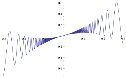
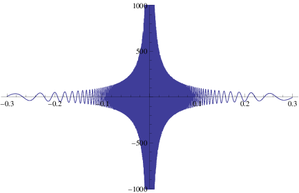
If $f:{\mathbb{R}}\longrightarrow{\mathbb{R}}$ is differentiable and $f^{\prime}(x_{0})\neq 0$, this does not imply that $f$ is monotonic in some neighbourhood of $x_{0}$. This is illustrated by the function [9, p. 37]

$$f:{\mathbb{R}}\longrightarrow{\mathbb{R}},\quad f(x):=\left\{\begin{array}[]{ll}x+\alpha x^{2}\sin\frac{1}{x^{2}}&\mbox{ for }x\neq 0\\[2.0pt] 0&\mbox{ for }x=0,\end{array}\right.\qquad\mbox{ where }\alpha\neq 0$$

which is differentiable everywhere with $f^{\prime}(0)=1\neq 0$, but is not monotonic (hence not one-to-one) on any neighbourhood of 0 since $f^{\prime}$ assumes both positive and negative values there. In fact, $f^{\prime}$ is unbounded in both directions on each such neighbourhood (see Figure 2).

By Darboux’s intermediate value theorem for derivatives, if a derivative $f^{\prime}$ is not continuous at some point $x_{0}$, then $x_{0}$ has to be an oscillation point of $f^{\prime}$ (i.e. there is a certain interval $J$ of positive length such that $f^{\prime}$ assumes all values in $J$ in arbitrarily small neighbourhoods of $x_{0}$). In the usual examples for this situation (like $x\mapsto x^{2}\sin\frac{1}{x}$), $f^{\prime}$ oscillates in both directions, above and below $f^{\prime}(x_{0})$, i.e. for arbitrary small neighbourhoods $U$ of $x_{0}$, $f^{\prime}(x_{0})$ is an inner point of $f^{\prime}(U)$.

The function

$$f(x):=x^{3}+\int_{0}^{x}\left|\cos\frac{1}{t}\right|^{1/|t|}\,dt$$

(a slight variation of the function from Example 1) is an example of a differentiable function $f:{\mathbb{R}}\longrightarrow{\mathbb{R}}$ which satisfies $f^{\prime}(0)=0<f^{\prime}(x)$ for all $x\in{\mathbb{R}}\setminus\left\{0\right\}$ and whose derivative $f^{\prime}$ is not continuous at 0, i.e. $f^{\prime}$ oscillates only above $f^{\prime}(0)$ (see Figure 3). In other words, $f^{\prime}$ has even a strict minimum at the origin. Here, $f^{\prime}(0)=0$ is not obvious, so we provide the details.

Proof. The function $t\mapsto\left|\cos\frac{1}{t}\right|^{1/|t|}$ is bounded and continuous almost everywhere, so by Lebesgue’s criterion it is integrable (even in the sense of Riemann) on compact intervals. Therefore, $f$ is well-defined. For $x\neq 0$ it is clear from the fundamental theorem of calculus that $f^{\prime}(x)=3x^{2}+\left|\cos\frac{1}{x}\right|^{1/|x|}>0$.

So it remains to show that $f^{\prime}(0)=0$. For this purpose we substitute $u:=\frac{1}{t}$ to write $f(x)$ in the form

$$f(x)=x^{3}+\int_{1/x}^{\infty}\frac{|\cos u|^{u}}{u^{2}}\,du\qquad\mbox{ for }x>0$$

and consider the points

$$a_{k}:=k\pi,\qquad b_{k}:=\left(k+\frac{1}{k^{1/4}}\right)\cdot\pi,\qquad c_{k}:=\left(k+1-\frac{1}{k^{1/4}}\right)\cdot\pi\qquad(k\in{\rm I\!N}).$$

For $k\geq 16$ we have $a_{k}\leq b_{k}\leq c_{k}\leq a_{k+1}$,

$$\int_{a_{k}}^{b_{k}}\frac{|\cos u|^{u}}{u^{2}}\,du\leq\frac{b_{k}-a_{k}}{a_{k}^{2}}=\frac{1}{\pi\cdot k^{9/4}}$$

and

$$\int_{c_{k}}^{a_{k+1}}\frac{|\cos u|^{u}}{u^{2}}\,du\leq\frac{a_{k+1}-c_{k}}{c_{k}^{2}}\leq\frac{1}{\pi\cdot k^{9/4}}.$$

Furthermore, using the estimate $\cos y\leq 1-\frac{y^{2}}{4}$ for $0\leq y\leq\frac{\pi}{2}$, for $k\geq 16$ we obtain

$$\int_{b_{k}}^{c_{k}}\frac{|\cos u|^{u}}{u^{2}}\,du\leq\frac{c_{k}-b_{k}}{b_{k}^{2}}\cdot\left(\cos\frac{\pi}{k^{1/4}}\right)^{b_{k}}\leq\frac{1}{\pi k^{2}}\cdot\left(1-\frac{\pi^{2}}{4\sqrt{k}}\right)^{k\pi}.$$

Here, $\lim_{k\to\infty}\left(1-\frac{\pi^{2}}{4\sqrt{k}}\right)^{\sqrt{k}\pi}=e^{-\pi^{3}/4}<1$, so if we set $\alpha:=\frac{1}{2}\cdot\left(1+e^{-\pi^{3}/4}\right)$, then there exists some $N_{0}\geq 16$ such that

$$\left(1-\frac{\pi^{2}}{4\sqrt{k}}\right)^{\sqrt{k}\pi}\leq\alpha\qquad\mbox{ for all }k\geq N_{0},$$

and we get

$$\int_{b_{k}}^{c_{k}}\frac{|\cos u|^{u}}{u^{2}}\,du\leq\frac{1}{\pi k^{2}}\cdot\alpha^{\sqrt{k}}\qquad\mbox{ for all }k\geq N_{0}.$$

Combining these estimates, for all $N\geq N_{0}-1$ we deduce

	$\displaystyle 0$	$\displaystyle\leq$	$\displaystyle\int_{(N+1)\pi}^{\infty}\frac{|\cos u|^{u}}{u^{2}}\,du$
		$\displaystyle=$	$\displaystyle\sum_{k=N+1}^{\infty}\left(\int_{a_{k}}^{b_{k}}\frac{|\cos u|^{u}}{u^{2}}\,du+\int_{b_{k}}^{c_{k}}\frac{|\cos u|^{u}}{u^{2}}\,du+\int_{c_{k}}^{a_{k+1}}\frac{|\cos u|^{u}}{u^{2}}\,du\right)$
		$\displaystyle\leq$	$\displaystyle\sum_{k=N+1}^{\infty}\left(\frac{2}{\pi\cdot k^{9/4}}+\frac{1}{\pi k^{2}}\cdot\alpha^{\sqrt{k}}\right)\leq\frac{2}{\pi}\int_{N}^{\infty}\frac{dx}{x^{9/4}}+\frac{1}{\pi}\int_{N}^{\infty}\frac{\alpha^{\sqrt{x}}}{\sqrt{x}}\;dx$
		$\displaystyle=$	$\displaystyle\frac{8}{5\pi}\cdot\frac{1}{N^{5/4}}+\frac{2}{\pi}\int_{\sqrt{N}}^{\infty}\alpha{{}^{y}}\,dy=\frac{8}{5\pi}\cdot\frac{1}{N^{5/4}}+\frac{2\alpha^{\sqrt{N}}}{\pi\log\frac{1}{\alpha}}.$

Now let some $x>0$ be given. W.l.o.g. we may assume $x<\frac{1}{N_{0}\pi}$. Then there exists some $N_{x}\in{\rm I\!N}$, $N_{x}\geq N_{0}$ such that $\frac{1}{(N_{x}+1)\pi}<x\leq\frac{1}{N_{x}\pi}$. Here for $x\to 0+$ we have $N_{x}\longrightarrow\infty$, so we obtain

	$\displaystyle 0$	$\displaystyle\leq$	$\displaystyle\frac{f(x)}{x}\leq x^{2}+(N_{x}+1)\pi\cdot\int_{N_{x}\pi}^{\infty}\frac{\left|\cos u\right|^{u}}{u^{2}}\,du$
		$\displaystyle\leq$	$\displaystyle x^{2}+\frac{8}{5}\cdot\frac{N_{x}+1}{(N_{x}-1)^{5/4}}+\frac{2}{\log\frac{1}{\alpha}}\cdot(N_{x}+1)\cdot\alpha^{\sqrt{N_{x}-1}}\quad\longrightarrow 0\mbox{ for }x\to 0+.$

This shows that $\frac{f(x)}{x}\longrightarrow 0$ for $x\to 0+$. In view of $f(-x)=-f(x)$ the same holds for $x\to 0-$. So $f$ is differentiable at 0 with $f^{\prime}(0)=0$.

It is clear that $f^{\prime}$ is not continuous at 0. $\blacksquare$

This example can be easily modified such that $f^{\prime}$ is even unbounded near the origin (and still oscillates only in the positive direction, i.e. between 0 and $\infty$), by setting

$$f(x):=\int_{0}^{x}\frac{1}{\sqrt{|t|}}\cdot\left|\cos\frac{1}{t}\right|^{1/|t|^{2}}\,dt.$$

Furthermore, functions with the properties discussed in this item can also be constructed as integral functions of piecewise linear functions, having increasingly thinner and increasingly higher peaks which accumulate at the origin but this might be considered less elegant than the examples discussed above.

In calculus textbooks, there are various definitions of an inflection point¹¹ 1 For a more detailed discussion of five different definitions of inflection point we refer to [15, Section 5.5]. Here we just want to point out some noteworthy aspects.. Maybe the most common one (see, for example [11, p. 195], [12, p. 147] and [17, p. 186]) is the following one.

• (D1)

  A continuous function $f:[a,b]\longrightarrow{\mathbb{R}}$ has an inflection point at $x_{0}\in(a,b)$ if $f$ is strictly convex on one side of $x_{0}$ (more precisely, in a certain interval $(x_{0}-\delta,x_{0})$ resp. $(x_{0},x_{0}+\delta)$) and strictly concave on the other side.

According to this definition also a function like

$$f(x):=\left\{\begin{array}[]{ll}x^{2}&\mbox{ for }x<0\\ \sqrt{x}&\mbox{ for }x\geq 0\end{array}\right.$$

(1)

has an inflection point at $x=0$ though it is not differentiable there.

Sometimes (for example in [1, p. 388]) also the following definition can be found:

• (D2)

  A function $f:[a,b]\longrightarrow{\mathbb{R}}$ has an inflection point at $x_{0}\in(a,b)$ if $f$ is differentiable at $x_{0}$ and if the graph of $f$ is strictly above the tangent line $x\mapsto f(x_{0})+f^{\prime}(x_{0})\cdot(x-x_{0})$ on one side of $x_{0}$ and strictly below this tangent line on the other side.

This definition does not apply to the function in (1), but in the case of functions which are differentiable at $x_{0}$, it is more general than the first definition. For example, if we set

$$f(x):=x^{3}+{\rm sgn}(x)\cdot x^{2}\sin^{2}\frac{1}{x}=\left\{\begin{array}[]{ll}x^{3}+x^{2}\sin^{2}\frac{1}{x}&\mbox{ for }x>0,\\ 0&\mbox{ for }x=0,\\ x^{3}-x^{2}\sin^{2}\frac{1}{x}&\mbox{ for }x<0,\end{array}\right.$$

then $f$ is differentiable at $x=0$ with $f^{\prime}(0)=0$, $f(x)>0$ for all $x>0$ and $f(x)<0$ for all $x<0$, so $f$ has an inflection point at $x=0$ in the sense of (D2). However, $f$ is neither convex nor concave in $(0,\delta)$ for any $\delta>0$, and the same holds in the intervals $(-\delta,0)$ (see Figure 4).

Definition (D2) even applies to functions which are not continuous in any neighbourhood of the inflection point. For example, with this definition the function

$$f(x):=\left\{\begin{array}[]{ll}x^{3}&\mbox{ for }x\in{\mathbb{Q}},\\ x^{5}&\mbox{ for }x\in{\mathbb{R}}\setminus{\mathbb{Q}}.\end{array}\right.$$

(whose graph looks like the union of the graphs of $x\mapsto x^{3}$ and of $x\mapsto x^{5}$, though this is of course a visual illusion) has an inflection point at $x=0$.

Finally, some authors (for example [8, p. 150]) prefer the following definition which is, however, the least general one since it is restricted to functions that are differentiable everywhere (not just at the inflection point):

• (D3)

  A differentiable function $f:[a,b]\longrightarrow{\mathbb{R}}$ has an inflection point at $x_{0}\in\;(a,b)$ if $f^{\prime}$ has a strict local extremum at $x_{0}$.

For functions that are differentiable everywhere, definition (D3) is more general than (D1) but less general than (D2). More precisely, if $f:[a,b]\longrightarrow{\mathbb{R}}$ is differentiable, then

• •

  if $x_{0}\in\;(a,b)$ is an inflection point in the sense of (D1), it is also an inflection point in the sense of (D3) (since strict convexity resp. concavity can be described in terms of the first derivative being strictly increasing resp. decreasing),

• •

  and if it is an inflection point in the sense of (D3), it is also an inflection point in the sense of (D2) as easily seen by considering the function

  $$d(x):=f(x)-f(x_{0})-f^{\prime}(x_{0})(x-x_{0})$$

  which under the conditions of (D2) is strictly monotonic with a zero at $x_{0}$, hence changes its sign at $x=x_{0}$.

That an inflection point in the sense of (D2) need not be an inflection point in the sense of (D3) is again illustrated by the function from Figure 4. To find an example for an inflection point in the sense of (D3), but not in the sense of (D1), we recall that a strict local minimum doesn’t necessarily mean a change from monotonically decreasing to monotonically increasing as we know from Example 2. In fact, the desired example is provided by an antiderivative of a function as in Example 2, say the function $f:{\mathbb{R}}\longrightarrow{\mathbb{R}}$ defined by

$$f(x):=\int_{0}^{x}t^{2}\left(1.1+\sin\frac{1}{t}\right)\,dt\qquad\mbox{ for }x\in{\mathbb{R}}.$$

(Here we have slightly modified the function from Example 2 in order to make the desired phenomenon more apparent in the graph. But it still has the very same properties: It has a strict extremum at the origin, but isn’t decreasing on one side nor decreasing on the other side of the extremum.)

There are certain analogies between infinite series and improper Riemann integrals of the form $\int_{0}^{\infty}f(t)\,dt$. For example, if $f:[0,\infty[\longrightarrow[0,\infty[$ is monotonically decreasing, then the convergence of the improper integral $\int_{0}^{\infty}f(t)\,dt$ is equivalent to the convergence of the series $\sum_{n=0}^{\infty}f(n)$.

Now if $\sum_{n=0}^{\infty}a_{n}$ is a convergent series, $(a_{n})_{n}$ necessarily converges to 0. This might (mis)lead to the conjecture that if the improper Riemann integral $\int_{0}^{\infty}f(t)\,dt$ converges (where $f$ is a continuous function) then $\lim_{t\to\infty}f(t)=0$. But this is wrong. On the contrary, the function

$$f(x):=x\sin(x^{3})$$

(Figure 6) shows that $f(x)$ can be even unbounded as $x\to\infty$ (cf. also [9, p. 46]). Here, to show the convergence of $\int_{0}^{\infty}f(t)\,dt$ we substitute $y:=t^{3}$ which gives

$$\int_{1}^{R}f(t)\,dt=\int_{1}^{R^{3}}\frac{\sin y}{3y^{1/3}}\,dy\qquad\mbox{ for all }R>0$$

and observe that the improper integral $\int_{1}^{\infty}\frac{\sin y}{3y^{1/3}}\,dy$ converges.

When talking about differentiable functions $f:[a;\infty)\longrightarrow{\mathbb{R}}$ with a certain asymptotic behaviour near $\infty$, say $\lim_{x\to\infty}f(x)=0$, the question arises how the derivative $f^{\prime}$ behaves near $\infty$. Probably some students will think that $f^{\prime}(x)$ is bound to tend to 0 as $x\to\infty$.

However, there’s no good reason to think so, as you can illustrate by the following analogy: If a small particle is trapped in a small room and we make this room smaller and smaller, this particle might still be able to move arbitrarily fast within this room (as long as it is able to accelerate and decelerate within very short times).

In fact, a simple counterexample is provided by the function

$$f(x):=\frac{\sin(x^{3})}{x}$$

which satisfies $\lim_{x\to\infty}f(x)=0$. Here $\lim_{x\to\infty}f^{\prime}(x)$ does not exist, and $f^{\prime}$ is even unbounded near $\infty$ (Figure 7). Actually, $f^{\prime}$ behaves very much like the function in Example 6.

It is more difficult to give a counterexample where $f$ is even monotonic, i.e. $f^{\prime}$ doesn’t change signs. Here a near relative of the function from Example 2 proves to be helpful: Choose an arbitrary $\varepsilon>0$ and define

$$f(x):=\int_{0}^{x}|\cos t|^{t^{2+\varepsilon}}\,dt\qquad\mbox{ for }x>0.$$

Then $f$ is differentiable on $(0;\infty)$ with non-negative derivative $f^{\prime}(x)=|\cos x|^{x^{2+\varepsilon}}$ (whose zeros are isolated), i.e. $f$ is strictly increasing, and $f^{\prime}(x)$ does not tend to 0 for $x\to\infty$. Furthermore, a reasoning similar to Example 4 shows that the improper integral $\int_{0}^{\infty}|\cos t|^{t^{2+\varepsilon}}\,dt=\lim_{x\to\infty}f(x)$ exists.

Proof. We consider the points

$$a_{k}:=k\pi,\qquad b_{k}:=\left(k+\frac{1}{k^{1+\varepsilon/4}}\right)\cdot\pi,\qquad c_{k}:=\left(k+1-\frac{1}{k^{1+\varepsilon/4}}\right)\cdot\pi$$

for $k\in{\rm I\!N}$. Then $a_{k}\leq b_{k}\leq c_{k}\leq a_{k+1}$ for $k$ large enough, and we can estimate

$$\int_{a_{k}}^{b_{k}}|\cos t|^{t^{2+\varepsilon}}\,dt\leq b_{k}-a_{k}=\frac{\pi}{k^{1+\varepsilon/4}},\qquad\int_{c_{k}}^{a_{k+1}}|\cos t|^{t^{2+\varepsilon}}\,dt\leq\frac{\pi}{k^{1+\varepsilon/4}},$$

$$\int_{b_{k}}^{c_{k}}|\cos t|^{t^{2+\varepsilon}}\,dt\leq(c_{k}-b_{k})\cdot\left(\cos\frac{\pi}{k^{1+\varepsilon/4}}\right)^{b_{k}^{2+\varepsilon}}\leq\pi\cdot\left(1-\frac{\pi^{2}}{4k^{2+\varepsilon/2}}\right)^{(k\pi)^{2+\varepsilon}}.$$

From $\lim_{k\to\infty}\left(1-\frac{\pi^{2}}{4k^{2+\varepsilon/2}}\right)^{k^{2+\varepsilon/2}}=e^{-\pi^{2}/4}<1$ we see that there is a constant $\alpha<1$ such that

$$\int_{b_{k}}^{c_{k}}|\cos t|^{t^{2+\varepsilon}}\,dt\leq\pi\cdot\alpha^{k^{\varepsilon/2}}$$

for $k$ sufficiently large. Here the series $\sum_{k=1}^{\infty}\frac{\pi}{k^{1+\varepsilon/4}}$ is obviously convergent, and the convergence of $\sum_{k=1}^{\infty}\alpha^{k^{\varepsilon/2}}$ follows from the convergence of the improper integral $\int_{1}^{\infty}\alpha^{x^{\varepsilon/2}}\,dx=\frac{2}{\varepsilon}\int_{1}^{\infty}\alpha^{y}y^{2/\varepsilon-1}\,dy$. Summarizing, we conclude that $\int_{0}^{\infty}|\cos t|^{t^{2+\varepsilon}}\,dt$ exists. $\blacksquare$

We set $I:=[-2,2]$, $B_{n}:=\left[\frac{1}{n+1},\frac{2n+1}{2n(n+1)}\right)$ and

$$A:=[-2,2]\setminus\left(\left\{0\right\}\cup\bigcup_{n=1}^{\infty}B_{n}\cup\bigcup_{n=1}^{\infty}(-B_{n})\right).$$

(Observe that $\frac{2n+1}{2n(n+1)}$ is just the middle of the interval $\left[\frac{1}{n+1},\frac{1}{n}\right]$.)

Then $A$ is an uncountable subset of ${\mathbb{R}}$, so by the Cantor-Bernstein-Schroeder theorem [10] there exists a one-to-one map $T$ of $[-2,-1]\;\cup\;[1,2]$ onto $A$. We define $f:[-2,2]\longrightarrow{\mathbb{R}}$ by

$$f(x):=\left\{\begin{array}[]{ll}0&\mbox{ for }x=0,\\[6.0pt] \frac{1}{n+1}+\frac{1}{2}\left(x-\frac{1}{n+1}\right)&\mbox{ for }\frac{1}{n+1}\leq x<\frac{1}{n},\\[6.0pt] -\frac{1}{n+1}+\frac{1}{2}\left(x+\frac{1}{n+1}\right)&\mbox{ for }-\frac{1}{n}<x\leq-\frac{1}{n+1},\\[6.0pt] T(x)&\mbox{ for }x\in[-2,-1]\;\cup\;[1,2].\end{array}\right.$$

The graph of $f$ in the interval $[0.05,0.6]$ is sketched in Figure 9. Obviously, $f(-x)=-f(x)$ for $-1<x<1$.

Since $f$ maps the intervals $\left[\frac{1}{n+1},\frac{1}{n}\right)$ linearly onto $B_{n}$, it is clear that $f$ maps $I$ onto itself in a one-to-one fashion. For any given $x\in\left[\frac{1}{n+1},\frac{1}{n}\right)$ we can write $x=\frac{1}{n+1}+\tau$ with $0\leq\tau<\frac{1}{n(n+1)}$, so we obtain

$$\frac{f(x)-f(0)}{x-0}=\frac{\frac{1}{n+1}+\frac{\tau}{2}}{\frac{1}{n+1}+\tau}=\frac{1+\frac{\tau}{2}(n+1)}{1+\tau(n+1)}\left\{\begin{array}[]{ll}\leq 1,\\[6.0pt] \geq\frac{1}{1+\frac{1}{n}}.\end{array}\right.$$

From this and the fact that $f$ is an odd function on $(-1,1)$ we see that the derivative $f^{\prime}(0)=1\neq 0$ exists. But $f^{-1}$ is not continuous at $y_{0}=f(0)=0$ since $f^{-1}(A)=[-2,-1]\;\cup\;[1,2]$ and since $0$ is an accumulation point of $A$. In particular, $f^{-1}$ cannot be differentiable at $y_{0}$.

References

- [1] T. Apostol: Calculus, Vol. 1, Blaisdell Publishing Company, New York London 1961
- [2] J. Appell: Analysis in examples and counterexamples. An introduction to the theory of real functions, Springer, Berlin 2009
- [3] J. Appell: Some counterexamples for your calculus course, Analysis (München) 31 (2011), 1-12
- [4] J. Appell; A.-K. Roos: Continuity, monotonicity, oscillation, variation: obvious and surprising aspects (Stetigkeit, Monotonie, Oszillation, Variation: Naheliegendes und Überraschendes), Math. Semesterber. 61 (2014), 233-248
- [5] D. Ball: An introduction to real analysis, Pergamon Press 1973
- [6] E. Behrends: Analysis, Vol. 1. A study book for a smooth transition from school to university. With the cooperation of students, 6th edition, Springer Spektrum, Wiesbaden 2015
- [7] O. Deiser: Analysis 1, 2nd edition, Springer Spektrum, Heidelberg 2013
- [8] F. Erwe: Differential- und Integralrechnung. Band 1: Elemente der Infinitesimalrechnung und Differentialrechnung, B.I.-Hochschultaschenbücher, Bibliographisches Institut, Mannheim 1962
- [9] B. Gelbaum; J. Olmsted: Counterexamples in Analysis, Holden-Day Inc. 1964
- [10] A. Hinkis: Proofs of the Cantor-Bernstein theorem. A mathematical excursion, Science Networks. Historical Studies 45, Birkhäuser/Springer, Basel 2013
- [11] G. Köhler: Analysis, Heldermann, Lemgo 2006
- [12] K. Königsberger: Analysis 1, 2nd edition, Springer, Berlin Heidelberg 1992
- [13] D. Meizler: Infinitesimal Calculus, Academon 1968 (Hebrew)
- [14] E. Moise: Calculus, Addison-Wesley, 1966
- [15] A.R. Rajwade; A.K. Bhandari: Surprises and counterexamples in real function theory, Texts and Readings in Mathematics 42. Hindustan Book Agency, New Delhi 2007
- [16] K. Ross: Elementary analysis: The theory of calculus, 2nd edition, Springer, New York 2013
- [17] S. Salas; E. Hille: Calculus. One and several variables (Calculus. Einführung in die Differential- und Integralrechnung, Spektrum, Heidelberg 1995
- [18] L. Zalcman: Positive derivatives and increasing functions, Elem. Math. 43 (1988), 120-121
Jürgen Grahl
University of Würzburg
97074 Würzburg
Germany
e-mail: grahl@mathematik.uni-wuerzburg.de
Shahar Nevo
Bar-Ilan University
Ramat-Gan 52900
Israel
e-mail: nevosh@math.biu.ac.il