On Genera of Curves from High-loop Generalized Unitarity Cuts

Consider a complex curve $C$ in $\mathbb{C}^{n}$, defined by polynomial equations

The polynomials $f_{1},\ldots f_{k}$ generate an ideal $J=\langle f_{1},\ldots f_{k}\rangle$. In the formal language, $C$ is the zero locus of $J$.

To discuss its topology, we need to extend $C$ to a projective curve $\mathcal{C}$ in $\mathbb{CP}^{n}$. Define homogenous coordinates by $z_{i}=Z_{i}/Z_{0}$, $\mathcal{C}$ is defined by homogenous polynomials

All such $F$’s generate a homogenous ideal $I$. In practice, to get $I$, we do not need to find the homogenous form of all polynomials in $J$. Instead, it is sufficient to consider the homogenous form of polynomials in the Gröbner basis of $J$, in a graded monomial order [38].

Furthermore, we assume that $\mathcal{C}$ is irreducible, i.e., cannot be written as the union of two different curves. Equivalently, it means that $I$ is a prime ideal [35]. For the cases of reducible curves, we consider the genus of each irreducible component. Irreducible components can be found by primary decomposition [35],

where all $I_{i}$’s are prime ideals. Primary decomposition technique has been used in high-loop unitarity cuts [29] [34] [31].

The arithmetic genus can be defined by the Hilbert polynomial of the quotient ring $S/I$, where $S=\mathbb{C}[Z_{0},Z_{1},\ldots Z_{k}]$. $S/I$ is a graded S-module,

There exists a unique polynomial $P(x)$ and a positive integer $N$ such that, for $n>N$, $n\in\mathbb{Z}$,

This polynomial is called Hilbert polynomial (of the projective curve $\mathcal{C}$). Then the arithmetic genus of $\mathcal{C}$ is defined to be

In practice, the Hilbert polynomial and arithmetic genus can be easily calculated by Gröbner basis method. In particular, for a plane curve, i.e. a curve in $\mathbb{CP}^{2}$, defined by one homogenous polynomial with degree $d$, the arithmetic genus is simply [35]

The arithmetic genus is not directly related to the topological properties of a curve, since intuitively it counts not only the number of handles but also the singular points. A singular point on $\mathcal{C}$ is a point $(a_{0},a_{1},....a_{n})$ such that the rank of the Jacobian matrix,

is less than $n-1$ [35], where $F_{i}$, $1\leq i\leq k$ are the generators of equations for the curve. A singular point on $\mathcal{C}$ is normal if all tangent lines on the singular point are distinct.

For a smooth curve, i.e., an irreducible projective curve without a singular point, we define the geometric genus to be its arithmetic genus [35]. For an irreducible projective curve $\mathcal{C}$ with singular points, there exists a smooth irreducible projective curve $\mathcal{\tilde{C}}$, which is the normalization of $\mathcal{C}$ [35],

We define the geometric genus of $\mathcal{C}$ to be the arithmetic genus of $\mathcal{\tilde{C}}$. This definition is consistent with the topological definition of the genus. In particular, for an irreducible plane curve with normal singular points only, the geometric genus is related to the arithmetic genus as

where $Sing(\mathcal{C})$ is the collection of all singular points $P$ on $\mathcal{C}$. $\mu_{P}$ is the multiplicity of $P$, i.e., the number of tangent lines at $P$. In practice, $Sing(\mathcal{C})$ can be found by computational algebraic geometry softwares, like Macaulay2 [37].

We may frequently re-parametrize a curve, and intuitively, the topological information should be invariant after re-parametrization. To realize the re-parametrization process rigorously, we introduce the concept of birational map: A rational map $r$ from the irreducible curves, $C_{1}$ and $C_{2}$, is a map from a non-empty open set of $C_{1}$ to $C_{2}$, such that, in terms of the coordinates, all components of $f$ are rational functions. A birational map $f$ between two irreducible curves is a rational map $f$ from $C_{1}$ to $C_{2}$ with an inverse rational map $g$ from $C_{2}$ to $C_{1}$, such that $gf$ is the identity map on an open set of $C_{1}$ and $fg$ is the identity map on an open set of $C_{2}$. The geometric genus is a birational invariant [35].

In particular, since $\mathbb{CP}^{1}$ has the genus zero, a project curve with $g_{G}>0$ is not birational to $\mathbb{CP}^{1}$. It implies that there is no rational parametrization for such a curve.

We present some simple examples on the genera of algebraic curves:

1. 1.

   $y^{2}=x^{3}+1$. This is a cubic plane curve. The corresponding projective curve is $Y^{2}Z=X^{3}+Z^{3}$. There is no singular point on the projective curve. The arithmetic genus is $(3-2)(3-1)/2=1$ and the geometric genus is also $1$. So this is an elliptic curve.

2. 2.

   $y^{2}=x^{3}+x^{2}$. This is also a cubic plane curve. The corresponding projective curve is $Y^{2}Z=X^{3}+X^{2}Z$. There is a singular point at $X=0,Y=0,Z=1$ and there are two distinct tangent lines at this point: $x-y=0$ and $x+y=0$. So this is an ordinary singular point with the multiplicity $2$. The arithmetic genus is still $1$ but the geometric genus is $1-2(2-1)/2=0$. So this is not an elliptic curve. We can blow up the singular point at $(x,y)=(0,0)$ as follows [35]: define a new variables $t$ via $y=xt$, and the equation becomes $-x^{2}(1-t^{2}+x)=0$. Factorize it and keep the curve part, we get a new curve $1-t^{2}+x=0$. This new curve is birational to the original curve, and is smooth. Since the new curve is conic, so we show that the original curve is birationally equivalent to a conic and can be rational parameterized.

3. 3.

   The projective curve,

   $$XT-YZ=0,\quad X^{2}Z+Y^{3}+YZT=0,\quad XZ^{2}+Y^{2}T+ZT^{2}=0$$

   (13)

   is non-singular [36] . From Macaulay2, we find that the arithmetic genus is $2$, so its geometric genus is also $2$.

There are many different ways to calculate the genus of an algebraic curve. In this paper, for the algebraic curves from unitarity cuts in two-loop and three-loop orders, we mainly use the relation between arithmetic genus and geometric genus for the computation. Explicitly, if the curve is non-singular, then we simply calculate its arithmetic genus and by the definition, it is the geometric genus. Otherwise, we birationally project the curve onto a plane, and then use (11) to determine the genus if all singular points are normal. If some singular points are not normal, we use the blow up process to resolve them, as described in [36].

Anther useful formula for curve genus computation is Riemann-Hurwitz formula [35]. Let $f:C_{1}\to C_{2}$ be a covering map between two irreducible complex curves $C_{1}$ and $C_{2}$, and $n$ is the degree of $f$. Then $g(C_{1})$ and $g(C_{2})$, the genera of $C_{1}$ and $C_{2}$ are related by

where $e_{P}$ is the ramification index of $P$. For all but finite points on $C_{1}$, the ramification index equals one so it is just a finite sum. Therefore if $g(C_{2})$ is known, we can get $g(C_{1})$ by counting the ramified points on $C_{1}$.

As a warm-up, we first analyze this simple diagram, in Figure.(1.a). The $7$ propagators are given by

There are $4$ propagators containing $\ell_{1}$ only, and from the on-shell equations $D_{i}=0$, we can completely fix the variables in $\ell_{1}$. These equations $D_{i}=0,i=1,2,3,4$ have two solutions. For each solution, since $\ell_{1}$ has already been completely fixed, we can treat it as a four-vector similar to an external momentum. Thus the on-shell propagators highlighted by dashed lines in Figure (1.a)

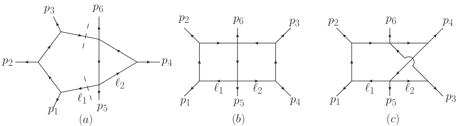
can be effectively treated as massless external momenta. Then for each solution, the result of two-loop planar pentagon-triangle diagram is the same as the result of the one-loop triangle diagram. It is associated with a genus-0 Riemann sphere. In some specific kinematic configurations where degeneracy exists, the topological picture becomes that of two Riemann spheres connected at a single point.

It is already known in [23] that on-shell equations of the two-loop double-box diagram, with six massive legs, define an one-dimensional elliptic curve which is associated with a genus-$1$ torus.

We can reproduce this result by directly computing the arithmetic genus and singular points of the curve. Taking the convention shown in Figure (1.b), the $7$ propagators can be written as,

In order to compute the arithmetic genus and singular points, we first rewrite above equations by expanding all momenta on a momentum basis. A simple analysis is as follows. We have variables $(x_{1},x_{2},x_{3},x_{4})$ for 4 components of $\ell_{1}$ and $(y_{1},y_{2},y_{3},y_{4})$ for 4 components of $\ell_{2}$. Using on-shell equations $D_{i}=0,\widetilde{D}_{i}=0$, we can eliminate $2$ variables of $x_{i}$ and $2$ of $y_{i}$, and get $3$ quadratic polynomials $Q_{1}=Q_{1}(x_{1},x_{2})$, $Q_{2}=Q_{2}(y_{1},y_{2})$, $Q_{3}=Q_{3}(x_{1},x_{2},y_{1},y_{2})$. This can be done by Yang’s BasisDet package[29]. We can further eliminate $2$ variables and $2$ equations via Gröbner basis method and get a plane curve. This plane curve has degree $8$, so the arithmetic genus is

There are $10$ singular points, of which $8$ have the multiplicity $\mu_{P}=2$ and $2$ have the multiplicity $\mu_{P}=4$, so the geometric genus is

This result is consistent with that in [23].

Another explicit way of getting an equivalent plane curve can be taken as follows. Through coordinate transformation it is easy to rewrite $Q_{1}\to Q^{\prime}_{1}=x^{\prime}_{1}x^{\prime}_{2}-c_{1}$, $Q_{2}\to Q^{\prime}_{2}=y^{\prime}_{1}y^{\prime}_{2}-c_{2}$, so we can do the following substitution $x^{\prime}_{1}=c_{1}/x^{\prime}_{2},y^{\prime}_{1}=c_{2}/y^{\prime}_{2}$ in $Q_{3}$. The resulting $Q^{\prime}_{3}=n(x^{\prime}_{2},y^{\prime}_{2})/d(x^{\prime}_{2},y^{\prime}_{2})$ is a meromorphic function which is equivalent to original equations, and the numerator $n(x^{\prime}_{2},y^{\prime}_{2})$ defines a plane curve. This plane curve $n(x^{\prime}_{2},y^{\prime}_{2})$ has the degree $4$, so we have $g_{A}=3$. There are $2$ singular points of the multiplicity $\mu_{P}=2$, thus we get the geometric genus $g_{G}=3-2=1$. This result again agrees with that given in [23].

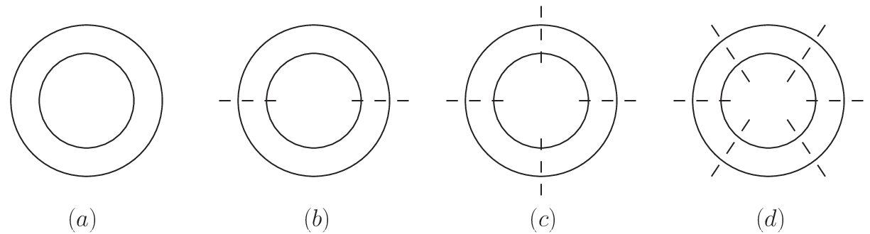
The topological pictures of genus of degenerate algebraic curves under specific kinematic configurations can be easily found, because in degenerate limit the tube shrinks to point, and there is only one handle for the torus. The contraction will break the handle, and we should get genus-0 Riemann spheres connected at points. Equations of each irreducible branch can be obtained by Macaulay2 [37] via primary decomposition. By computing the arithmetic genus and singular points, we found that their geometric genera are indeed zero. The $3$ kinds of contraction shown in Figure (2) describe topological pictures of degenerate algebraic curves under all possible specific kinematic configurations. There are $2$, $4$ or $6$ Riemann spheres connected by points along dashed lines where tubes shrink, and linked adjacently into a chain. This is exactly the picture described in [23].

For the two-loop non-planar crossed-box diagram, the explicit form of propagators for generic kinematics is very complicated. Abstractly, we write the $7$ propagators as,

From above propagators, we can at most get $4$ polynomials which are linear in $\ell$,

and $3$ polynomials which are quadratic in $\ell$,

If we use momentum basis $e_{1},e_{2},e_{3},e_{4}$ to expand loop momenta as,

and the $8$ variables are taken as the expansion coefficients $(x_{1},x_{2},x_{3},x_{4})$ and $(y_{1},y_{2},y_{3},y_{4})$, then there will be quadratic terms from products of two loop momenta $\ell_{i}\ell_{j}$, and linear terms from products like $\ell_{i}p_{j}$. Systematically we can generate the Gröbner basis by $7$ on-shell equations $D_{i}=\widetilde{D}_{i}=\widehat{D}_{i}=0$, and find all linear terms in the Gröbner basis. We can remove as many variables as possible by solving these linear terms, and express other terms with remaining variables. In this case, we get an equivalent but simplified polynomial equation system. A more explicit way is to solve linear equations $L_{i}=0$, and express $4$ variables as linear functions of remaining $4$ variables. Substituting solutions back to quadratic polynomial equations $Q_{i}=0$, we get an alternate algebraic set. It is possible to analyze the three quadratic equations by algebraic geometry program such as Macaulay2 [37].

Let us consider the two-loop non-planar crossed-box diagram drawn in Figure (1.c). All external momenta are general, and we construct momentum basis $e_{i}$ from $p_{1},p_{3}$¹¹ 1 Momentum basis $e_{i}$ have the following orthogonal and normalization relations $e_{1}e_{2}=e_{3}e_{4}=1$, otherwise $0$. The explicit form can be found by Gram-Schmidt process.. External momenta are expanded as

where $\alpha,\beta,\gamma$ are the projection coefficients of momenta on the corresponding momentum basis, for example $\alpha_{11}=p_{1}e_{2},\alpha_{12}=p_{1}e_{1}$. Using this expansion, the four linear polynomials $L_{i}$ become

and the three quadratic polynomials $Q_{i}$ become

The equations until now are still simple, but after solving $L_{i}=0$ and substituting solutions back to $Q_{i}$, they will become quadratic polynomials with complicate coefficients of $\alpha,\beta,\gamma$. Anyway, $Q_{i}$’s are still $3$ quadratic polynomials in $4$ variables, and they define a one-dimensional curve.

As we have mentioned, different definitions of momentum basis and variables, and the choices of choosing remaining variables after solving linear equations, will describe different curves. But they are all birationally equivalent. Birational invariants will stay the same in each description. So we project the three quadratic equations onto a plane curve. By a coordinate transformation, we can eliminate $2$ equations as well as $2$ variables, and the resulting equation defines a plane curve describing an equivalent algebraic set. This equation has the degree $d=8$, so the arithmetic genus is,

The singular points can be obtained directly from the definition, i.e., for projective plane curve defined by homogeneous polynomial $P(x,y,z)$ of degree $d$, the singular points are solutions of equations

For this plane curve, there are 18 normal singular points of the multiplicity $\mu_{P}=2$, so the geometric genus is again

Another way of getting a plane curve from original on-shell equations is to use the elimination process via Gröbner basis method. We can use BasisDet package to generate on-shell equations, where the variables are defined as independent Lorentz Invariant Scalar Products (ISPs) of loop momentum and external momentum. Using these cut equations and Gröbner basis associated with them, we get a plane curve. The degree of the plane curve is $8$, so we have $g_{A}=21$. There are $18$ normal singular points of the multiplicity $2$, so again we get the geometric genus $g_{G}=21-18=3$.

To summarize, the maximal unitarity cut of two-loop non-planar crossed-box diagram can fix $7$ components of loop momenta, and the solution set of on-shell equations is described by a free parameter corresponding to the remaining one degree of freedom. The variety is associated with a genus-$3$ Riemann surface.

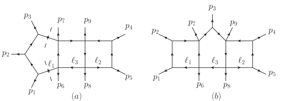
We consider the generic pentagon-box-box diagram with $9$ massive external legs, as shown in Figure (5.a).

The $11$ propagators are given by

The $11$ on-shell equations $D_{i}=\widetilde{D}_{i}=\bar{D}_{i}=\widehat{D}_{i}=0$ of maximal unitarity cut define an algebraic curve, and its topology is actually simple. To see this, note that $4$ on-shell equations $D_{i}=0$ contain only $\ell_{1}$, and we can solve them first. Since $\ell_{1}$ has $4$ components, these $4$ equations will completely fix $\ell_{1}$. Explicitly, after solving $3$ linear equations from $D_{i}=0$, the remaining one becomes a quadratic equation of a single variable. This equation will give two solutions for $\ell_{1}$, and on each solution, $\ell_{1}$ is completed fixed. Hence $\ell_{1}$ can be treated as a $4$-vector similar to external momenta. The remaining $11-4=7$ cut equations for $l_{2}$ and $l_{3}$ are the same as the two-loop double-box case.

More explicitly, for each solution of $\ell_{1}$, the on-shell propagators highlighted by dashed lines in Figure (5.a) can be treated as massless external momenta. So the discussion reduces to the two-loop double-box diagram with general kinematics if $p_{6},p_{7}$ are not absent. As we know it is a genus-$1$ torus. In some specific kinematic configurations of $(p_{4},p_{5},p_{6},p_{7},p_{8},p_{9})$, the algebraic curves are degenerate, and the topological pictures are given by genus-$0$ Riemann spheres connected at points and linked in a chain, just as the two-loop double-box diagram. The two solutions of $\ell_{1}$ are separated.

On-shell equations of the three-loop box-pentagon-box diagram are much more complicated. Naive elimination of linear equations will generate $5$ quadratic equations in $6$ variables, and they define a one-dimensional curve. More explicitly, we consider the generic box-pentagon-box diagram with $9$ massive external momenta as shown in Figure (5.b). Among the $11$ propagators, there are $3$ containing $\ell_{1}$ only

$3$ containing $\ell_{2}$ only

and $3$ containing $\ell_{3}$ only

The remaining two propagators contain terms of mixed loop momenta, and they are given by,

We have $4$ variables for each loop momentum, denoted as $(x_{1},x_{2},x_{3},x_{4})$ for $\ell_{1}$, $(y_{1},y_{2},y_{3},y_{4})$ for $\ell_{2}$ and $(z_{1},z_{2},z_{3},z_{4})$ for $\ell_{3}$. As usual, for each loop momentum we have $2$ linear equations, and by solving them, we can eliminate $2$ variables and $2$ equations. So finally we get $5$ quadratic polynomials,

Notice that $Q_{1}(x_{3},x_{4})=0$, $Q_{2}(y_{3},y_{4})=0$ and $Q_{3}(z_{3},z_{4})=0$ are conics. So it is always possible to find rational parametrization for each loop momentum, and express them by one free parameter as $\ell_{1}=\ell_{1}(x)$, $\ell_{2}=\ell_{2}(y)$ and $\ell_{3}=\ell_{3}(z)$²² 2 By coordinate transformation, we can rewrite a non-degenerate conic $Q(x,y)=0$ in the form $Q^{\prime}(x^{\prime},y^{\prime})=x^{\prime}y^{\prime}-c=0$, and express one parameter as a rational function of the other as $x^{\prime}=c/y^{\prime}$. So the loop momentum can be expanded as a rational function of a single variable.. The remaining two equations $\widehat{D}_{0}$ and $\widehat{D}_{1}$ are meromorphic functions after substituting $\ell_{i}$ back, and the numerators define an algebraic plane curve as,

For generic massive external momenta, $a_{i}$ and $b_{i}$ are quadratic polynomials. We can eliminate $z$ by computing the resultant of these two equations to get a plane curve $F(x,y)$=0. This plane curve is birationally equivalent to (33) via the inverse map,

so they have the same geometric genus. For generic kinematic configurations, the plane curve $F(x,y)$ has the degree $8$, so the arithmetic genus is

There are $4$ singular points of the multiplicity $\mu_{P}=2$, and $2$ singular points of the multiplicity $\mu_{P}=4$, so the geometric genus is given by

So this is a genus 5 curve.

Alternatively, we can also find the genus of (33) by Riemann-Hurwitz formula (14)³³ 3 We thank Simon Caron-Huot for the discussion of using this formula.. Let $\mathcal{C}$ be the complex curve defined by (33). The projection $f:(x,y,z)\mapsto z$ is a covering map from $\mathcal{C}$ to the complex plane of $z$. For all but finite points, this is a four-fold covering so the degree of the map is $4$. We determine the ramified points as follows:

1. 1.

   Consider the first equation in (33) as a quadratic equation for $x$ and the discriminant is $\Delta_{1}(z)$. For a fixed value of $z$, there are two corresponding $x$ unless $\Delta_{1}(z)$ vanishes. We can checked that $\Delta_{1}(z)=0$ have four distinct roots on the $z$ plane, namely $z_{1}$, $z_{2}$, $z_{3}$ and $z_{4}$.

2. 2.

   Consider the second equation in (33) as a quadratic equation for $y$ and the discriminant is $\Delta_{2}(z)$. We can checked that $\Delta_{2}(z)=0$ have four distinct roots on the $z$ plane, namely $z_{5}$, $z_{6}$, $z_{7}$ and $z_{8}$.

3. 3.

   We checked $z_{i}$’s are all disctint, $i=1,\ldots,8$. Hence for each $z_{i}$, $i=1,\ldots 4$, there are two corresponding points on $\mathcal{C}$, namely $(x_{i},y_{i}^{(1)},z_{i})$ and $(x_{i},y_{i}^{(2)},z_{i})$. For each $z_{i}$, $i=5,\ldots 8$, there are two corresponding points on $\mathcal{C}$, namely $(x_{i}^{(1)},y_{i},z_{i})$ and $(x_{i}^{(2)},y_{i},z_{i})$. So there are $2\times 4+2\times 4=16$ ramified points on $\mathcal{C}$ and each point has the ramification index $2$.

Then we can use Riemann-Hurwitz formula (14) and the fact that the complex plane has the genus zero,

Again we get the same conclusion that the curve has the genus $5$.

Finally, we can also find the genus with the help of two-loop-diagram genus information. If we forget the cut equations involves $l_{2}$ for a while, the rest equations form the hepta-cut equations of the two-loop massive double box diagram. Intuitively, it is clear that if all propagators involving $l_{2}$ are pinched, the resulting diagram is the massive double box. Explicitly, neglect the second equation in (33) and we find that the remaining equation,

References

- (1) R. Britto, F. Cachazo and B. Feng, Nucl. Phys. B 715, 499 (2005) [hep-th/0412308].
- (2) R. Britto, F. Cachazo, B. Feng and E. Witten, Phys. Rev. Lett. 94, 181602 (2005) [hep-th/0501052].
- (3) L. D. Landau, Nucl. Phys. 13, 181 (1959); S. Mandelstam, Phys. Rev. 112, 1344 (1958); S. Mandelstam, Phys. Rev. 115, 1741 (1959); R. E. Cutkosky, J. Math. Phys. 1, 429 (1960).
- (4) Z. Bern, L. J. Dixon, D. C. Dunbar and D. A. Kosower, Nucl. Phys. B 435, 59 (1995) [arXiv:hep-ph/9409265].
- (5) Z. Bern, L. J. Dixon, D. C. Dunbar and D. A. Kosower, Nucl. Phys. B 425, 217 (1994) [arXiv:hep-ph/9403226].
- (6) N. Arkani-Hamed, F. Cachazo and J. Kaplan, JHEP 1009, 016 (2010) [arXiv:0808.1446 [hep-th]].
- (7) C. Anastasiou, R. Britto, B. Feng, Z. Kunszt and P. Mastrolia, Phys. Lett. B 645, 213 (2007) [arXiv:hep-ph/0609191].
- (8) C. Anastasiou, R. Britto, B. Feng, Z. Kunszt and P. Mastrolia, JHEP 0703, 111 (2007) [arXiv:hep-ph/0612277].
- (9) R. Britto, J. Phys. A 44, 454006 (2011) [arXiv:1012.4493 [hep-th]].
- (10) R. Britto, F. Cachazo and B. Feng, Nucl. Phys. B 725, 275 (2005) [arXiv:hep-th/0412103].
- (11) R. Britto, E. Buchbinder, F. Cachazo and B. Feng, Phys. Rev. D 72, 065012 (2005) [arXiv:hep-ph/0503132].
- (12)
F. V. Tkachov, Phys. Lett. B 100, 65 (1981);
K. G. Chetyrkin and F. V. Tkachov, Nucl. Phys. B 192, 159 (1981).
S. Laporta, Phys. Lett. B 504, 188 (2001) [hep-ph/0102032].
S. Laporta, Int. J. Mod. Phys. A 15, 5087 (2000) [hep-ph/0102033]. - (13) G. Ossola, C. G. Papadopoulos and R. Pittau, Nucl. Phys. B 763, 147 (2007) [hep-ph/0609007].
- (14) D. Forde, Phys. Rev. D 75, 125019 (2007) [arXiv:0704.1835 [hep-ph]].
- (15) R. K. Ellis, W. T. Giele and Z. Kunszt, JHEP 0803, 003 (2008) [arXiv:0708.2398 [hep-ph]].
- (16) W. B. Kilgore, arXiv:0711.5015 [hep-ph].
- (17) W. T. Giele, Z. Kunszt and K. Melnikov, JHEP 0804, 049 (2008) [arXiv:0801.2237 [hep-ph]].
- (18) G. Ossola, C. G. Papadopoulos and R. Pittau, JHEP 0805, 004 (2008) [arXiv:0802.1876 [hep-ph]].
- (19) S. D. Badger, JHEP 0901, 049 (2009) [arXiv:0806.4600 [hep-ph]].
- (20) J. Gluza, K. Kajda and D. A. Kosower, Phys. Rev. D 83, 045012 (2011) [arXiv:1009.0472 [hep-th]].
- (21) D. A. Kosower and K. J. Larsen, Phys. Rev. D 85, 045017 (2012) [arXiv:1108.1180 [hep-th]].
- (22) K. J. Larsen, arXiv:1205.0297 [hep-th].
- (23) S. Caron-Huot and K. J. Larsen, arXiv:1205.0801 [hep-ph].
- (24) R. H. P. Kleiss, I. Malamos, C. G. Papadopoulos and R. Verheyen, arXiv:1206.4180 [hep-ph].
- (25) H. Johansson, D. A. Kosower and K. J. Larsen, arXiv:1208.1754 [hep-th].
- (26) H. Johansson, D. A. Kosower and K. J. Larsen, arXiv:1212.2132 [hep-th].
- (27) P. Mastrolia and G. Ossola, JHEP 1111, 014 (2011) [arXiv:1107.6041 [hep-ph]].
- (28) S. Badger, H. Frellesvig and Y. Zhang, JHEP 1204, 055 (2012) [arXiv:1202.2019 [hep-ph]].
- (29) Y. Zhang, JHEP 1209, 042 (2012) [arXiv:1205.5707 [hep-ph]].
- (30) P. Mastrolia, E. Mirabella, G. Ossola and T. Peraro, Phys. Lett. B 718, 173 (2012) [arXiv:1205.7087 [hep-ph]].
- (31) B. Feng and R. Huang, arXiv:1209.3747 [hep-ph].
- (32) P. Mastrolia, E. Mirabella, G. Ossola and T. Peraro, arXiv:1209.4319 [hep-ph].
- (33) P. Mastrolia, E. Mirabella, G. Ossola, T. Peraro and H. van Deurzen, arXiv:1209.5678 [hep-ph].
- (34) S. Badger, H. Frellesvig and Y. Zhang, JHEP 1208, 065 (2012) [arXiv:1207.2976 [hep-ph]].
- (35) R. Hartshorne, Algebraic geometry. Springer-Verlag, New York, 1977. Graduate Texts in Mathematics, No. 52.
- (36) D. Perrin, Algebraic geometry. Universitext. Springer-Verlag London Ltd., London, 2008. An introduction, Translated from the 1995 French original by Catriona Maclean.
- (37) D. R. Grayson, M.E. Stillman, ”Macaulay2, a software system for research in algebraic geometry.” Available at http://www.math.uiuc.edu/Macaulay2/.
- (38) D. Cox, J. Little, and D. O’Shea, Ideals, varieties, and algorithms. Undergraduate Texts in Mathematics. Springer, New York, Third ed., 2007. An introduction to computational algebraic geometry and commutative algebra.