Beyond Worst-case Analysis for Joins with Minesweeper
Abstract
We describe a new algorithm, Minesweeper, that is able to satisfy stronger runtime guarantees than previous join algorithms (colloquially, ‘beyond worst-case guarantees’) for data in indexed search trees. Our first contribution is developing a framework to measure this stronger notion of complexity, which we call certificate complexity, that extends notions of Barbay et al. and Demaine et al.; a certificate is a set of propositional formulae that certifies that the output is correct. This notion captures a natural class of join algorithms. In addition, the certificate allows us to define a strictly stronger notion of runtime complexity than traditional worst-case guarantees. Our second contribution is to develop a dichotomy theorem for the certificate-based notion of complexity. Roughly, we show that Minesweeper evaluates -acyclic queries in time linear in the certificate plus the output size, while for any -cyclic query there is some instance that takes superlinear time in the certificate (and for which the output is no larger than the certificate size). We also extend our certificate-complexity analysis to queries with bounded treewidth and the triangle query.
1 Introduction
Efficiently evaluating relational joins is one of the most well-studied problems in relational database theory and practice. Joins are a key component of problems in constraint satisfaction, artificial intelligence, motif finding, geometry, and others. This paper presents a new join algorithm, called Minesweeper, for joining relations that are stored in order data structures, such as B-trees. Under some mild technical assumptions, Minesweeper is able to achieve stronger runtime guarantees than previous join algorithms.
The Minesweeper algorithm is based on a simple idea. When data are stored in an index, successive tuples indicate gaps, i.e., regions in the output space of the join where no possible output tuples exist. Minesweeper maintains gaps that it discovers during execution and infers where to look next. In turn, these gaps may indicate that a large number of tuples in the base relations cannot contribute to the output of the join, so Minesweeper can efficiently skip over such tuples without reading them. By using an appropriate data structure to store the gaps, Minesweeper guarantees that we can find at least one point in the output space that needs to be explored, given the gaps so far. The key technical challenges are the design of this data structure, called the constraint data structure, and the analysis of the join algorithm under a more stringent runtime complexity measure.
To measure our stronger notion of runtime, we introduce the notion of a certificate for an instance of a join problem: essentially, a certificate is a set of comparisons between elements of the input relations that certify that the join output is exactly as claimed. We use the certificate as a measure of the difficulty of a particular instance of a join problem. That is, our goal is to find algorithms whose running times can be bounded by some function of the smallest certificate size for a particular input instance. Our notion has two key properties:
- •
Certificate complexity captures the computation performed by widely implemented join algorithms. We observe that the set of comparisons made by any join algorithm that interacts with the data by comparing elements of the input relations (implicitly) constructs a certificate. Examples of such join algorithms are index-nested-loop join, sort-merge join, hash join,11 1 Within a -factor, an ordered tree can simulate a hash table. grace join, and block-nested loop join. Hence, our results provide a lower bound for this class of algorithms, as any such algorithm must take at least as many steps as the number of comparisons in a smallest certificate for the instance.
- •
Certificate complexity is a strictly finer notion of complexity than traditional worst-case data complexity. In particular, we show that there is always a certificate that is no larger than the input size. In some cases, the certificate may be much smaller (even constant-sized for arbitrarily large inputs).
These two properties allow us to model a common situation in which indexes allow one to answer a query without reading all of the data—a notion that traditional worst-case analysis is too coarse to capture. We believe ours is the first beyond worst-case analysis of join queries.
Throughout, we assume that all input relations are indexed consistently with a particular ordering of all attributes called the global attribute order (GAO). In effect, this assumption means that we restrict ourselves to algorithms that compare elements in GAO order. This model, for example, excludes the possibility that a relation will be accessed using indexes with multiple search keys during query evaluation.
With this restriction, our main technical results are as follows. Given a -acyclic query we show that there is some GAO such that Minesweeper runs in time that is essentially optimal in the certificate-sense, i.e., in time , where is a smallest certificate for the problem instance, is the output size, and hides factors that depend (perhaps exponentially) on the query size and at most logarithmically on the input size.22 2 The exponential dependence on the query is similar to traditional data complexity; the logarithmic dependence on the data is an unavoidable technical necessity (see Appendix C). Assuming the 3SUM conjecture, this boundary is tight, in the sense that any -cyclic query (and any GAO) there are some family of instances that require a run-time of for any where . For -acyclic join queries, which are the more traditional notion of acyclicity in database theory and a strictly larger class than -acyclic queries, Yannakakis’s seminal join algorithm has a worst-case running time that is linear in the input size plus output size (in data complexity). However, we show that in the certificate world, this boundary has changed: assuming the exponential time hypothesis, the runtime of any algorithm for -acyclic queries cannot be bounded by any polynomial in .33 3 In Appendix J, we show that both worst-case optimal algorithms [40, 53] and Yannakakis’s algorithm run in time for -acyclic queries on some family of instances.
We also describe how to extend our results to notions of treewidth. Recall that any ordering of attributes can be used to construct a tree decomposition. Given a GAO that induces a tree decomposition with an (induced) treewidth , Minesweeper runs in time . In particular, for a query with treewidth , there is always a GAO that achieves . Moreover, we show that no algorithm (comparison-based or not) can improve this exponent by more than a constant factor in . However, our algorithm does not have an optimal exponent: for the special case of the popular triangle query, we introduce a more sophisticated data structure that allows us to run in time , while Minesweeper runs in time .
Outline of the Remaining Sections
In Section 2, we describe the notion of a certificate and formally state our main technical problem and results. In Section 3, we give an overview of the main technical ideas of Minesweeper, including a complete description of our algorithm and its associated data structures. In Section 4, we describe the analysis of Minesweeper for -acyclic queries. In Section 5, we then describe how to extend the analysis to queries with low-treewidth and the triangle query. In Section 6, we discuss related work. Most of the technical details are provided in the appendix.
2 Problem and Main Result
Roughly, the main problem we study is:
Given a natural join query and a database instance , compute in time , where is the smallest “certificate" that certifies that the output is as claimed by the algorithm and .
We will assume that all relations in the input are already indexed. Ideally, we aim for . We make this problem precise in this section.
2.1 The inputs to Minesweeper
We assume a set of attributes and denote the domain of attribute as . Throughout this paper, without loss of generality, we assume that all attributes are on domain . We define three items: (1) the global attribute order; (2) our notation for order; and (3) our model for how the data are indexed.
The Global Attribute Order
Minesweeper evaluates a given natural join query consisting of a set of relations indexed in a way that is consistent with an ordering of all attributes occurring in that we call the global attribute order (GAO). To avoid burdening the notation, we assume that the GAO is simply the order . We assume that all relations are stored in ordered search trees (e.g., B-trees) where the search key for this tree is consistent with this global order. For example, is consistent, while is not.
Tuple-Order Notation
We will extensively reason about the relative order of tuples and describe notation to facilitate the arguments. For a relation where is such that if , we define an index tuple to be a tuple of positive integers, where . Such tuples index tuples in the relation . We define their meaning inductively. If , then denotes the ’th smallest value in the set . Inductively, define to be the ’th smallest value in the set
For example, if then , , , and .
We use the following convention to simplify the algorithm’s description: for any index tuple ,
| (1) | |||||
| (2) |
Model of Indexes
The relation is indexed such that the values of various attributes of tuples from can be accessed using index tuples. We assume appropriate size information is stored so that we know what the correct ranges of the ’s are; for example, following the notation described above, the correct range is for every . With the convention specified in (1) and (2), and are out-of-range coordinates. These coordinates are used for the sake of brevity only; an index tuple, by definition, cannot contain out-of-range coordinates.
The index structure for supports the query , which takes as input an index tuple of length and a value , and returns a pair of coordinates such that
- •
- •
, and
- •
(resp. ) is the maximum (resp. minimum) index satisfying this condition.
Note that it is possible for , which holds when . Moreover, we assume throughout that FindGap runs in time . This model captures widely used indexes including a B-tree [45, Ch.10] or a Trie [53].
2.2 Certificates
We define a certificate, which is a set of comparisons that certifies the output is exactly as claimed. We do not want the comparisons to depend on the specific values in the instance, only their order. To facilitate that, we think of as a variable that can be mapped to specific domain value by a database instance.44 4 We use variables as a perhaps more intuitive, succinct way to describe the underlying morphisms. These variables are only defined for valid index tuples as imposed by the input instance described in the previous section.
A database instance instantiates all variables , where , is an index tuple in relation . (In particular, the input database instance described in the previous section is such a database instance.) We use to denote the instantiation of the variable . Note that each such variable is on the domain of some attribute ; for short, we call such variable an -variable. A database instance fills in specific values to the nodes of the search tree structures of the input relations.
Example 2.1.
Consider the query on the input instance defined by and . This instance can be viewed as defining the following variables: , , , , , and , . Another database instance can define the same index variables but using different constants, in particular, set , , , , and , .
We next formalize the notion of certificates. Consider an input instance to Minesweeper, consisting of the query , the GAO , and a set of relations already indexed consistently with the GAO.
Definition 2.2 (Argument).
An argument for the input instance is a set of symbolic comparisons of the form
| (3) |
and and are two index tuples55 5 Note again that the index tuples are constructed from the input instance as described in the previous section. such that and are both -variables for some , and . Note that we allow .66 6 Equality constraints between index tuples from same relation is required to guarantee that certificates are no longer than the input, see property (ii) below. A database instance satisfies an argument if is true for every comparison in the argument .
An index tuple for a relation is called a full index tuple if . Let be a database instance for the problem. Then, the full index tuple is said to contribute to an output tuple if the tuple is exactly the projection of onto attributes in . A collection of full index tuples is said to be a witness for if has exactly one full index tuple from each relation , and all index tuples in contribute to the same .
Definition 2.3 (Certificate).
An argument for the input instance is called a certificate iff the following condition is satisfied: if and are two database instances of the problem both of which satisfy , then every witness for is a witness for and vice versa. The size of a certificate is the number of comparisons in it.
Example 2.4.
Continuing with Example 2.1. Fix an , the argument is a certificate for . For every database, such as and in the example, that satisfies the two equalities, the set of witnesses are the same, i.e., the sets and for . Notice we do not need to spell out all of the outputs in the certificate.
Consider the instance in which , . While is very similar to , does not satisfy the certificate since . The certificate also does not apply to from Example 2.1, since defines a different set of variables from , e.g., is defined in , but not in .
Properties of optimal certificates
We list three important facts about , a minimum-sized certificate:
- (i)
The set of comparisons issued by a very natural class of (non-deterministic) comparison-based join algorithms is a certificate; this result not only justifies the definition of certificates, but also shows that is a lowerbound for the runtime of any comparison-based join algorithm.
- (ii)
can be shown to be at most linear in the input size no matter what the data and the GAO are, and in many cases can even be of constant size. Hence, running time measured in is a strictly finer notion of runtime complexity than input-based runtimes; and
- (iii)
depends on the data and the GAO.
We explain the above facts more formally in the following two propositions. The proofs of the propositions can be found in Appendix B.
Proposition 2.5 (Certificate size as run-time lowerbound of comparison-based algorithms).
Let be a join query whose input relations are already indexed consistent with a GAO as described in Section 2.1. Consider any comparison-based join algorithm that only does comparisons of the form shown in (3). Then, the set of comparisons performed during execution of the algorithm is a certificate. In particular, if is an optimal certificate for the problem, then the algorithm must run in time at least .
Proposition 2.6 (Upper bound on optimal certificate size).
Let be a general join query on relations and attributes. Let be the total number of tuples from all input relations. Then, no matter what the input data and the GAO are, we have , where .
In Appendix B, we present examples to demonstrate that can vary any where from to , that the input data or the GAO can change the certificate size, and that same-relation comparisons are needed.
2.3 Main Results
Given a set of input relations already indexed consistent with a fixed GAO, we wish to compute the natural join of these relations as quickly as possible. As illustrated in the previous section, a runtime approaching is optimal among comparison-based algorithms. Furthermore, runtimes as a function of can be sublinear in the input size. Ideally, one would like a join algorithm running in -time. However, such a runtime is impossible because for many instances the output size is superlinear in the input size, while is at most linear in the input size. Hence, we will aim for runtimes of the form , where is the output size and is some function; a runtime of is essentially optimal.
Our algorithm, called Minesweeper, is a general-purpose join algorithm. Our main results analyze its runtime behavior on various classes of queries in the certificate complexity model. Recall that -acyclic (often just acyclic) is the standard notion of (hypergraph) acyclicity in database theory [1, p. 128]. A query is -acyclic, a stronger notion, if every subquery of obtained by removing atoms from remains -acyclic. For completeness, we include these definitions and examples in Appendix A.
Let be the input size, the number of attributes, the number of relations, the output size, the maximum arity of input relations, and any optimal certificate for the instance. Our key results are as follows.
Theorem 2.7.
Suppose the input query is -acyclic. Then there is some GAO such that Minesweeper computes its output in time .
As is standard in database theory, we ignore the dependency on the query size, and the above theorem states that Minesweeper runs in time .77 7 For -acyclic queries with a fixed GAO, our results are loose; our best upper bound the complexity uses the treewidth from Section 5.
What about -cyclic queries? The short answer is no: we cannot achieve this guarantee. It is obvious that any join algorithm will take time . Using SUM-hardness, a well-known complexity-theoretic assumption [44], we are able to show the following.
Proposition 2.8.
Unless the SUM problem can be solved in sub-quadratic time, for any -cyclic query in any GAO, there does not exist an algorithm that runs in time for any on all instances.
We extend our analysis of Minesweeper to queries that have bounded treewidth and to triangle queries in Section 5. These results are technically involved and we only highlight the main technical challenges.
3 The Minesweeper Algorithm
We begin with an overview of the main ideas and technical challenges of the Minesweeper algorithm. Intuitively, Minesweeper probes into the space of all possible output tuples, and explores the gaps in this space where there is no output tuples. These gaps are encoded by a technical notion called constraints, which we describe next. (For illustration, we present complete end-to-end results for set intersection and the bow-tie query in Appendix H and I.)
3.1 Notation for Minesweeper
We need some notation to describe our algorithm. Define the output space of the query to be the space , where is the domain of attribute .88 8 Recall, we assume for simplicity. By definition, a tuple is an output tuple if and only if , and , for all , where is the set of attributes in .
Constraints
A constraint is an -dimensional vector of the following form: where for every . In other words, each constraint is a vector consisting of three types of components:
- (1)
open-interval component on the attribute (for some ) and ,
- (2)
wildcard or component, and
- (3)
equality component of the type .
In any constraint, there is exactly one interval component. All components after the interval component are wildcards. Hence, we will often not write down the wildcard components that come after the interval component. The prefix that comes before the interval component is called a pattern, which consists of any number of wildcards and equality components. The equality components encode the coordinates of the axis parallel affine planes containing the gap. For example, in three dimensions the constraint can be viewed as the region between the affine hyperplanes and ; and the constraint can be viewed as the strip inside the plane between the line and . We encode these gaps syntactically to facilitate efficient insertion, deletion, and merging.
Let be an arbitrary tuple from the output space, and be a constraint. Then, is said to satisfy constraint if for every one of the following holds: (1) , (2) and , or (3) and . We say a tuple is active with respect to a set of constraints if does not satisfy any constraint in the set (Geometrically, no constraint covers the point ).
3.2 A High-level Overview of Minesweeper
We break Minesweeper in two components: (1) a special data structure called the constraint data structure (CDS), and (2) an algorithm that uses this data structure. Algorithm 1 gives a high-level overview of how Minesweeper works, which we will make precise in the next section.
The CDS stores the constraints already discovered during execution. For example, consider the query
If Minesweeper determines that and , then we can deduce that there is no tuple in the output that has a value in the open interval . This observation is encoded as a constraint . A key challenge with the CDS is to efficiently find an active tuple , given a set of constraints already stored in the CDS.
The outer algorithm queries the CDS to find active tuples and then probes the input relations. If there is no active , the algorithm terminates. Given an active , Minesweeper makes queries into the index structures of the input relations. These queries either report that is an output tuple, in which case is output, or they discover constraints that are then inserted into the CDS. Intuitively, the queries into the index structures are crafted so that at least one of the constraints that is returned is responsible for ruling out in any optimal certificate.
We first describe the interface of the CDS and then the outer algorithm which uses the CDS.
3.3 The CDS
The CDS is a data structure that implements two functions as efficiently as possible: (1) takes a new constraint and inserts it into the data structure, and (2) returns an active tuple with respect to all constraints that have been inserted into the CDS, or null if no such exists.
Implementation
To support these operations, we implement the CDS using a tree structure called ConstraintTree, which is a tree with at most levels, one for each of the attributes following the GAO. Figure 1 illustrates such a tree. More details are provided in Appendix E.

Each node in the CDS corresponds to a prefix (i.e. pattern) of constraints; each node has two data structures:
(1) is a sorted list with one entry per child of in the underlying tree. Each entry in the sorted list is labeled with an element of and has a pointer to the subtree rooted at the corresponding child. There are two exceptions: (1) if is a leaf then , and (2) each has at most one additional child node labeled with .
(2) is a sorted list of disjoint open intervals under that corresponding attribute. A key property is that given a value we can, in logarithmic time, output the smallest value that is not covered by any interval in (via the Next function). We will maintain the invariant that, for every node in a ConstraintTree, none of the labels in is contained in an interval in .
The following lemma is straightforward hence we omit the proof. Note that when we insert a new interval that overlaps existing intervals and/or contains values in equalities, we will have to merge them and/or remove the entries in equalities; and hence the cost is amortized.
Proposition 3.1.
The operation can be implemented in amortized time , where is total number of constraint vectors already inserted.
3.4 The outer algorithm
Algorithm 2 contains all the details that were missing from the high-level view of Algorithm 1. Appendix D.1 has a complete run of Minesweeper on a specific query. Appendices H and I have the complete end-to-end descriptions of two specific queries, which help clarify the general algorithm. We prove the following result.
Theorem 3.2.
Let denote the input size, the number of output tuples, , and
Let be any optimal certificate for the input instance. Then, the total runtime of Algorithm 2 is
where is the total time taken by the constraint data structure. The algorithm inserts constraints to CDS and issues calls to .
Our proof strategy bounds the number of iterations of the algorithm using an amortized analysis. We pay for each probe point returned by the CDS by either charging a comparison in the certificate or by charging an output tuple. If is an output tuple, we charge the output tuple. If is not an output tuple, then we observe that at least one of the constraints we discovered must rule out . Recall that each constraint is essentially a pair of elements from some base relation. If one element from each such pair is not involved in any comparison in , then we can perturb the instance slightly by moving the comparison-free element to align with . This means does not have enough information to rule out as an output tuple, reaching a contradiction. Hence when is not an output tuple, essentially some gap must map to a pair of comparisons. Finally, using the geometry of the gaps, we show that each comparison is charged at most times and each output tuple is charged times. Thus, in total the number of iterations is .
When is an optimal-size certificate, the runtime above is about linear in plus the total time the CDS takes. Note, however, that can be very small, even constant. Hence, we basically shift all of the burden of join evaluation to the CDS. Thus, one should not hope that there is an efficient CDS for general queries:
Theorem 3.3 (Limitation of any CDS).
Unless the exponential time hypothesis is wrong, no constraint data structure can process the constraints and the probe point accesses in time polynomial (independent of the query) in the number of constraints inserted and probe points accessed.
Complete proofs of the above theorems are included in Appendix D. In the next sections, we analyze the CDS, specifically the function . Our analysis exploits properties of the query and the GAO for -acyclic and bounded treewidth queries.
4 -acyclic queries
We describe how to implement getProbePoint for -acyclic queries. In particular, we show that there is some GAO that helps implement getProbePoint in amortized logarithmic time. Hence, by Theorem 3.2 our running time is , which we argued previously is essentially optimal.
4.1 Overview
Recall that given a set of intervals, getProbePoint returns an active tuple , i.e., a tuple that does not satisfy any of the constraints stored in the CDS. Essentially, during execution there may be a large number of constraints, and getProbePoint needs to answer an alternating sequence of constraint satisfaction problems and insertions. The question is: how do we split this work between insertion time and querying time?
In Minesweeper, we take a lazy approach: we insert all the constraints without doing any cleanup on the CDS. Then, when getProbePoint is called Minesweeper might have to do hard work to return a new active tuple, applying memoization along the way so the heavy labor does not have to be repeated in the future. When the GAO has a special structure, this strategy helps keep every CDS operation at amortized logarithmic time. We first give an example to build intuition about how our lazy approach works.
Example 4.1.
Consider a query with three attributes , and suppose the constraints that are inserted into the CDS are
- (i)
for all ,
- (ii)
for all ,
- (iii)
for ,
- (iv)
and .
There are constraints, and there is no active tuple of the form for . Without memoization, the brute-force strategy will take time , because for every pair , the algorithm will have to verify in time that the constraints forbid all , the constraints forbid all , and the constraint forbid .
But we can do better by remembering inferences that we have made. Fix a value . Minesweeper recognizes in -time that there is no for which is active. Minesweeper is slightly smarter: it looks at constraints of the type (for ) and concludes in -time that every tuple satisfying those constraints also satisfies the constraint . Minesweeper remembers this inference by inserting the inferred constraint into the CDS. Then, for , it takes only -time to conclude that no tuple of the form can be active. It does this inference by inserting constraint , which is merged with to become . Overall, we need only -time to reach the same conclusion as the brute-force strategy.
4.2 Patterns
Recall that getProbePoint returns a tuple such that does not satisfy any of the constraints stored in the CDS. We find by computing , one value at a time, backtracking if necessary. We need some notation to describe the algorithm and the properties that we exploit.
Let be an integer. A vector for which is called a pattern. The number is the length of the pattern. If then it is an equality component of the pattern, while is a wildcard component of the pattern.
A node at depth in the tree ConstraintTree can be identified by a pattern of length corresponding naturally to the labels on the path from the root of ConstraintTree down to node . The pattern for node is denoted by . In particular, , the empty pattern.
Let be a pattern. Then, a specialization of is another pattern of the same length for which whenever . In other words, we can get a specialization of by changing some of the components into equality components. If is a specialization of , then is a generalization of . For two nodes and of the CDS, if is a specialization of , then we also say that node is a specialization of node .
The specialization relation defines a partially ordered set. When is a specialization of , we write . If in addition we know , then we write .
Let be the principal filter generated by in this partial order, i.e., it is the set of all nodes of the CDS such that is a generalization of and that . The key property of constraints that we exploit is summarized by the following proposition.
Proposition 4.2.
Using the notation above, for a -acyclic query, there exists a GAO such that for each the principal filter is a chain.
Recall that a chain is a totally ordered set. In particular, has a smallest pattern (or bottom pattern). Note that these patterns in might come from constraints inserted from relations, constraints inserted by the outputs of the join, or even constraints inserted due to backtracking. Thinking of the constraints geometrically, this condition means that the constraints form a collection of axis-aligned affine subspaces of where one is contained inside another.
In Appendix F, we prove Proposition 4.2 using a result of Brouwer and Kolen [15]. The class of GAOs in the proposition is called a nested elimination order. We show that there exists a GAO that is a nested elimination order if and only if the query is -acyclic. We also show that -acyclicity and this GAO can be found in polynomial time.
4.3 The getProbePoint Algorithm
Algorithm 3 describes getProbePoint algorithm specialized to -acyclic queries. In turn, this algorithm uses Algorithm 4, which is responsible for efficiently inferring constraints imposed by patterns above this level. We walk through the steps of the algorithm below.
Initially, let be the root node of the CDS. We set . This is the smallest value that does not belong to any interval stored in . We work under the implicit assumption that any interval inserted into ConstraintTree that contains must be of the form , for some . This is because the domain values are in . In particular, if then the constraints cover the entire output space and null can be returned.
Inductively, let , , be the prefix of we have built thus far. Our goal is to compute . What we need to find is a value such that does not belong to the intervals stored in for every node . For this, we call algorithm 4 that uses Prop. 4.2 to efficiently find or return that there is no such . We defer its explanation for the moment. We only note that if such a cannot be found (i.e. if is returned after the search), then we have to backtrack because what that means is that every tuple that begins with the prefix satisfies some constraint stored in ConstraintTree. Line 17 of Algorithm 3 shows how we backtrack. In particular, we save this information (by inserting a new constraint into the CDS) in Line 17 to avoid ever exploring this path again.
Next Chain Value.
The key to Algorithm 4 is that such a can be found efficiently since one only needs to look through a chain of constraint sets. We write if and there is no pattern such that . Every interval from a node higher up in the chain infers an interval at a node lower in the chain. For instance, in Example 4.1, the chain consists of three nodes , , and . Further, every constraint of the form infers a more specialized constraint of the form , which in turns infers a constraint of the form . Hence, if we infer every single constraint downward from the top pattern to the bottom pattern, we will be spending a lot of time. The idea of Algorithm 4 is to infer as large of an interval as possible from a node higher in the chain before specializing it down. Our algorithm will ensure that whenever we infer a new constraint (line 17 of Algorithm 4), this constraint subsumes an old constraint which will never be charged again in a future inference.
4.4 Runtime Analysis
The proofs of the following main results are in Appendix F.
Lemma 4.3.
Suppose the input query is -acyclic. Then, there exists a GAO such that each of the two operations getProbePoint and InsConstraint of ConstraintTree takes amortized time , where is the total number of constraints ever inserted.
The above lemma and Theorem 3.2 leads directly to one of our main results.
Corollary 4.4 (Restatement of Theorem 2.7).
Suppose the input query is -acyclic then there exists a GAO such that Minesweeper computes its output in time
In particular, its data-complexity runtime is essentially optimal in the certificate complexity world: .
Beyond -acyclic queries, we show that we cannot do better modulo a well-known complexity theoretic assumption.
Proposition 4.5 (Re-statement of Proposition 2.8).
Unless the SUM problem can be solved in sub-quadratic time, for any -cyclic query in any GAO, there does not exist an algorithm that runs in time for any on all instances.
Comparison with Worst-Case Optimal Algorithms
It is natural to wonder if Yannakakis’ worst-case optimal algorithm for -acyclic queries or the worst-case optimal algorithms of [40] (henceforth, NPRR) or [53] (henceforth LFTJ) can achieve runtimes of for -acyclic queries. We outline the intuition about why this cannot be the case.
Yannakakis’ algorithm performs pairwise semijoin reducers. If we pick an instance where such that there is a relation pair involved each with size , then Yannakakis’s algorithm will exceed the bound. For NPRR and LFTJ, consider the family of instances in which one computes all paths of length (some constant) in a directed graph (this can be realized by a “path" query of length where the relations are the edge set of ). Now consider the case where the longest path in has size at most . In this case the output is empty and since each relation is , we have and by Corollary 4.4, we will run in time . Hence, when has many paths (at least ) of length at most , then both NPRR and LFTJ will have to explore all paths leading to an runtime.
Appendix J presents a rich family of -acyclic queries and a family of instances that combines both of the ideas above to show that all the three worst-case optimal algorithms can have arbitrarily worse runtime than Minesweeper. In particular, even running those worst-case algorithms in parallel is not able to achieve the certificate-based guarantees.
5 Extensions
We extend in two ways: queries with bounded tree width and we describe faster algorithms for the triangle query.
5.1 Queries with bounded tree-width
While Proposition 2.8 shows that -time is not achievable for -cyclic queries, we are able to show the following analog of the treewidth-based runtime under the traditional worst-case complexity notion [19, 6].
Theorem 5.1 (Minesweeper for bounded treewidth queries).
Suppose the GAO has elimination width bounded by , Then, Minesweeper runs in time
In particular, if we ignore the dependence on the query size, the runtime is . Further, if the input query has treewidth bounded by , then there exists a GAO for which Minesweeper runs in the above time.
The overall structure of the algorithm remains identical to the -acyclic case, the only change is in getProbePoint. The getProbePoint algorithm for general queries remains very similar in structure to that of the -acyclic case (Algorithm 3), and if the input query is -acyclic (with a nested elimination order as the GAO), then the general getProbePoint algorithm is exactly Algorithm 3. The new issue we have to deal with is the fact that the poset at each depth is not necessarily a chain. Our solution is simple: we mimic the behavior of Algorithm 3 on a shadow of that is a chain and make use of both the algorithm and the analysis for the -acyclic case. Appendix G contains all the algorithm details, and the proofs of the above theorem, along with the following negative result.
It is natural to wonder if Theorem 5.1 is tight. In addition to the obvious dependency, the next result indicates that the dependence on also cannot be avoided, even if we just look at the class of -acyclic queries.
Proposition 5.2.
Unless the exponential time hypothesis is false, for every large enough constant , there is an -acyclic query for which there is no algorithm with runtime . Further, has treewidth .
Our analysis of Minesweeper is off by at most in the exponent.
Proposition 5.3.
For every , there exists an (-acyclic) query with treewidth with the following property. For every possible global ordering of attributes, there exists an (infinite family of) instance on which the Minesweeper algorithm takes time.
5.2 An implementation of Minesweeper
| Query | com-Orkut | soc-Epinions1 | soc-LiveJournal1 | |||
|---|---|---|---|---|---|---|
| Star | 352M | 214K | 1.5M | 1,067 | 207M | 172K |
| -path | 352M | 119K | 1.5M | 842 | 207M | 138K |
| Tree | 469M | 2.8M | 2M | 3,441 | 276M | 2.7M |
With the help of LogicBlox, we implemented Minesweeper inside the LogicBlox engine. Our results are preliminary: it is implemented for main memory data and all experiments are run in a multi-threaded mode. We run three queries: a star query, a small path query, and a tree query, which are described below, on three data sets Orkut online social network, Who-trusts-whom network of Epinions.com, and LiveJournal online social network.
- •
Star query: .
- •
-path query: .
- •
Tree query: .
For each query and each dataset, relation is a graph dataset, while every relation contains a subset of vertices from that graph dataset, where every vertex is chosen with a probability . Figure 2 shows the input size versus certificate size on different queries and different graph datasets. The certificate size is measured by counting the number of FindGap operations during computing join queries. These numbers show that certificate size is very small compared to input size and so it indicates that a practical implementation might be obtained.
5.3 The Triangle Query
We consider the triangle query that can be viewed as enumerating triangles in a given graph. Using the CDS described so far, Minesweeper computes this query in time , and this analysis is tight.99 9 A straightforward application of our more general analysis given in Theorem 5.1, which gives . The central inefficiency is that the CDS wastes time determining that many tuples with the same prefix have been ruled out by existing constraints. In particular, the CDS considers all possible pairs (of which there can be of them). By designing a smarter CDS, our improved CDS explores such pairs. We can prove the following result. (The details are in Appendix L.)
Theorem 5.4.
We can solve the triangle query, in time .
6 Related Work
Our work touches on a few different areas, and we structure the related work around each of these areas: join processing, certificates for set intersection, and complexity measures that are finer than worst-case complexity.
6.1 Join Processing
Many positive and negative results regarding conjunctive query evaluation also apply to natural join evaluation. On the negative side, both problems are -hard in terms of expression complexity [16], but are easier in terms of data complexity [50] (when the query is assumed to be of fixed size). They are -complete and thus unlikely to be fix-parameter tractable [43, 33].
On the positive side, a large class of conjunctive queries (and thus natural join queries) are tractable. In particular, the classes of acyclic queries and bounded treewidth queries can be evaluated efficiently [55, 17, 31, 27, 54]. For example, if is the query size, is the input size, and is the output size, then Yannakakis’ algorithm can evaluate acyclic natural join queries in time . Acyclic conjunctive queries can also be evaluated efficiently in the I/O model [42], and in the RAM model even when there are inequalities [54]. For queries with treewidth , it was recognized early on that a runtime of about is attainable [19, 28]. our result strictly generalizes these results. In Appendix J, we show that Yannakakis’ algorithm does not meet our notion of certificate optimality.
The notion of treewidth is loose for some queries. For instance, if we replicate each attribute times for every attribute, then the treewidth is inflated by a factor of ; but by considering all duplicate attributes as one big compound attribute the runtime should only be multiplied by a polynomial in and there should not be a factor of in the exponent of the runtime. Furthermore, there is an inherent incompatibility between treewidth and acyclicity: an acyclic query can have very large treewidth, yet is still tractable. A series of papers [17, 2, 32, 31, 27] refined the treewidth notion leading to generalized hyper treewidth [31] and ultimately fractional hypertree width [39], which allows for a unified view of tractable queries. (An acyclic query, for example, has fractional hypertree width at most .)
The fractional hypertree width notion comes out of a recent tight worst-case output size bound in terms of the input relation sizes [7]. An algorithm was presented that runs in time matching the bound, and thus it is worst-case optimal in [40]. Given a tree decomposition of the input query with the minimum fractional edge cover over all bags, we can run this algorithm on each bag, and then Yannakakis algorithm [55] on the resulting bag relations, obtaining a total runtime of , where is the fractional hyper treewidth. The leap-frog triejoin algorithm [53] is also worst-case optimal and runs fast in practice; it is based on the idea that we can efficiently skip unmatched intervals. The indices are also built or selected to be consistent with a chosen GAO. In the Appendix J, we show that neither Leapfrog nor the algorithm from [40] can achieve the certificate guarantees of Minesweeper for -acyclic queries.
Notions of acyclicity
There are at least five notions of acyclic hypergraphs, four of which were introduced early on in database theory (see e.g, [24]), and at least one new one introduced recently [22]. The five notions are not equivalent, but they form a strict hierarchy in the following way:
Acyclicity or -acyclicity [11, 12, 26, 29, 38] was recognized early on to be a very desirable property of data base schemes; in particular, it allows for a data-complexity optimal algorithm in the worst case [55]. However, an -acyclic hypergraph may have a sub-hypergraph that is not -acyclic. For example, if we take any hypergraph and add a hyperedge containing all vertices, we obtain an -acyclic hypergraph. This observation leads to the notion of -acyclicity: a hypergraph is -acyclic if and only if every one of its sub-hypergraph is (-) acyclic [24]. It was shown (relatively) recently [41] that sat is in for -acyclic CNF formulas and is -complete for -acyclic CNF formulas. Extending the result, it was shown that negative conjunctive queries are poly-time solvable if and only if it is -acyclic [14]. The separation between -acyclicity and -acyclicity showed up in logic [21], while Berge-acyclicity is restrictive and, thus far, is of only historical interest [13].
Graph triangle enumeration
In social network analysis, computing and listing the number of triangles in a graph is at the heart of the clustering coefficients and transitivity ratio. There are four decades of research on computing, estimating, bounding, and lowerbounding the number of triangles and the runtime for such algorithms [49, 37, 52, 51, 5, 36]. This problem can easily be reduced to a join query of the form .
6.2 Certificates for Intersection
The problem of finding the union and intersection of two sorted arrays using the fewest number of comparisons is well-studied, dated back to at least Hwang and Lin [35] since 1972. In fact, the idea of skipping elements using a binary-search jumping (or leap-frogging) strategy was already present in [35]. Demaine et al. [20] used the leap-frogging strategy for computing the intersection of sorted sets. They introduced the notion of proofs to capture the intrinsic complexity of such a problem. Then, the idea of gaps and certificate encoding were introduced to show that their algorithm is average case optimal. (See Appendix K for a more technical discussion.)
DLM’s notion of proof inspired another adaptive complexity notion for the set intersection problem called partition certificate by Barbay and Kenyon in [8, 9], where instead of a system of inequalities essentially a set of gaps is used to encode and verify the output. Barbay and Kenyon’s idea of a partition certificate is very close to the set of intervals that Minesweeper outputs. In the analysis of Minesweeper in Appendix H for the set intersection problem, we (implicitly) show a correspondence between these partition certificates and DLM’s style proofs. In addition to the fact that join queries are more general than set intersection, our notion of certificate is value-oblivious; our certificates do not depend on specific values in the domain, while Barbay-Kenyon’s partition certificate does.
It should be noted that these lines of inquiries are not only of theoretical interest. They have yielded good experimental results in text-datamining and text-compression[10].1010 10 We thank Jérémy Barbay for bringing these references to our attention.
6.3 Beyond Worst-case Complexity
There is a fairly large body of work on analyzing algorithms with more refined measures than worst-case complexity. (See, e.g., the excellent lectures by Roughgarden on this topic [46].) This section recalls the related works that are most closely related to ours.
A fair amount of work has been done in designing adaptive algorithms for sorting [23], where the goal is to design a sorting algorithm whose runtime (or the number of comparisons) matches a notion of difficulty of the instance (e.g. the number of inversions, the length of longest monotone subsequence and so on – the survey [23] lists at least eleven such measures of disorder). This line of work is similar to ours in the sense that the goal is to run in time proportional to the difficulty of the input. The major difference is that in these lines of work the main goal is to avoid the logarithmic factor over the linear runtime whereas in our work, our potential gains are of much higher order and we ignore log-factors.
Another related line of work is on self-improving algorithms of Ailon et al. [4], where the goal is to have an algorithm that runs on inputs that are drawn i.i.d. from an unknown distribution and in expectation converge to a runtime that is related to the entropy of the distribution. In some sense this setup is similar to online learning while our work requires worst-case per-instance guarantees.
The notion of instance optimal join algorithms was (to the best of our knowledge) first explicitly studied in the work of Fagin et al. [25]. The paper studies the problem of computing the top- objects, where the ranking is some aggregate of total ordering of objects according to different attributes. (It is assumed that the algorithm can only iterate through the list in sorted order of individual attribute scores.) The results in this paper are stronger than ours since Fagin et al. give -optimality ratio (as opposed to our -optimality ratio). On the other hand the results in the Fagin et al. paper are for a problem that is arguably narrower than the class we consider of join algorithms.
The only other paper with provable instance-optimal guarantees that we are aware of is the Afshani et al. results on some geometric problems [3]. Their quantitative results are somewhat incomparable to ours. On the one hand their results get a constant optimality ratio: on the other hand, the optimality ratio is only true for order oblivious comparison algorithms (while our results with optimality ratio hold against all comparison-based algorithms).
7 Conclusion and Future Work
We described the Minesweeper algorithm for processing join queries on data that is stored ordered in data structures modeling traditional relational databases. We showed that Minesweeper can achieve stronger runtime guarantees than previous algorithms; in particular, we believe Minesweeper is the first algorithm to offer beyond worst-case guarantees for joins. Our analysis is based on a notion of certificates, which provide a uniform measure of the difficulty of the problem that is independent of any algorithm. In particular, certificates are able to capture what we argue is a natural class of comparison-based join algorithms.
Our main technical result is that, for -acyclic queries there is some GAO such that Minesweeper runs in time that is linear in the certificate size. Thus, Minesweeper is optimal (up to an factor) among comparison-based algorithms. Moreover, the class of -acyclic queries is the boundary of complexity in that we show no algorithm for -cyclic queries runs in time linear in the certificate size. And so, we are able to completely characterize those queries that run in linear time for the certificate and hence are optimal in a strong sense. Conceptually, certificates change the complexity landscape for join processing as the analogous boundary for traditional worst-case complexity are -acyclic queries, for which we show that there is no polynomial bound in the certificate size (assuming the strong form of the exponential time hypothesis). We then considered how to extend our results using treewidth. We showed that our same Minesweeper algorithm obtains runtime for queries with treewidth . For the triangle query (with treewidth ), we presented a modified algorithm that runs in time .
Future Work
We are excited by the notion of certificate-based complexity for join algorithms; we see it as contributing to an emerging push beyond worst-case analysis in theoretical computer science. We hope there is future work in several directions for joins and certificate-based complexity.
Indexing and Certificates
The interplay between indexing and certificates may provide fertile ground for further research. For example, the certificate size depends on the order of attributes. In particular, a certificate in one order may be smaller than in another order. We do not yet have a handle on how the certificate-size changes for the same data in different orders. Ideally, one would know the smallest certificate size for any query and process in that order. Moreover, we do not know how to use of multiple access paths (eg. Btrees with different search keys) in either the analysis or the algorithm. These indexes may result in dramatically faster algorithms and new types of query optimization.
Fractional Covers
A second direction is that join processing has seen a slew of powerful techniques based on increasingly sophisticated notions of covers and decompositions for queries. We expect that such covers (hypergraph, fractional hypergraph, etc.) could be used to tighten and improve our bounds. For the triangle query, we have the fractional cover bound, i.e., . But is this possible for all queries?
Acknowledgments
We thank LogicBlox, Mahmoud Abo Khamis, Semih Salihoglu and Dan Suciu for many helpful conversations.
HQN’s work is partly supported by NSF grant CCF-1319402 and a gift from Logicblox. DTN’s work is partly supported by NSF grant CCF-0844796 and a gift from Logicblox. CR’s work on this project is generously supported by NSF CAREER Award under No. IIS-1353606, NSF award under No. CCF-1356918, the ONR under awards No. N000141210041 and No. N000141310129, Sloan Research Fellowship, Oracle, and Google. AR’s work is partly supported by NSF CAREER Award CCF-0844796, NSF grant CCF-1319402 and a gift from Logicblox.
References
- [1] S. Abiteboul, R. Hull, and V. Vianu, Foundations of Databases, Addison-Wesley, 1995.
- [2] I. Adler, G. Gottlob, and M. Grohe, Hypertree width and related hypergraph invariants, European J. Combin., 28 (2007).
- [3] P. Afshani, J. Barbay, and T. M. Chan, Instance-optimal geometric algorithms, in FOCS, 2009, pp. 129–138.
- [4] N. Ailon, B. Chazelle, K. L. Clarkson, D. Liu, W. Mulzer, and C. Seshadhri, Self-improving algorithms, SIAM J. Comput., 40 (2011), pp. 350–375.
- [5] N. Alon, On the number of subgraphs of prescribed type of graphs with a given number of edges, Israel J. Math., 38 (1981).
- [6] S. Arnborg and A. Proskurowski, Linear time algorithms for NP-hard problems restricted to partial -trees, Discrete Appl. Math., 23 (1989), pp. 11–24.
- [7] A. Atserias, M. Grohe, and D. Marx, Size bounds and query plans for relational joins, 2008, pp. 739–748.
- [8] J. Barbay and C. Kenyon, Adaptive intersection and t-threshold problems, in SODA, 2002, pp. 390–399.
- [9] , Alternation and redundancy analysis of the intersection problem, ACM Transactions on Algorithms, 4 (2008).
- [10] J. Barbay and A. López-Ortiz, Efficient algorithms for context query evaluation over a tagged corpus, in SCCC, M. Arenas and B. Bustos, eds., IEEE Computer Society, 2009, pp. 11–17.
- [11] C. Beeri, R. Fagin, D. Maier, A. Mendelzon, J. Ullman, and M. Yannakakis, Properties of acyclic database schemes, in STOC, New York, NY, USA, 1981, ACM, pp. 355–362.
- [12] C. Beeri, R. Fagin, D. Maier, and M. Yannakakis, On the desirability of acyclic database schemes, J. ACM, 30 (1983), pp. 479–513.
- [13] C. Berge, Graphs and Hypergraphs, Elsevier Science Ltd, 1985.
- [14] J. Brault-Baron, A Negative Conjunctive Query is Easy if and only if it is Beta-Acyclic, in CSL 12, vol. 16, 2012, pp. 137–151.
- [15] A. Brouwer and A. Kolen, A super-balanced hypergraph has a nest point, (1980). Tech. Report.
- [16] A. K. Chandra and P. M. Merlin, Optimal implementation of conjunctive queries in relational data bases, in STOC, 1977.
- [17] C. Chekuri and A. Rajaraman, Conjunctive query containment revisited, Theor. Comput. Sci., 239 (2000), pp. 211–229.
- [18] J. Chen, S. Lu, S.-H. Sze, and F. Zhang, Improved algorithms for path, matching, and packing problems, in SODA, 2007, pp. 298–307.
- [19] R. Dechter and J. Pearl, Tree clustering for constraint networks., Artificial Intelligence, 38 (1989), pp. 353–366.
- [20] E. D. Demaine, A. López-Ortiz, and J. I. Munro, Adaptive set intersections, unions, and differences, in SODA, 2000, pp. 743–752.
- [21] D. Duris, Hypergraph acyclicity and extension preservation theorems, in LICS, 2008, pp. 418–427.
- [22] , Some characterizations of and -acyclicity of hypergraphs., Information Processing Letters, 112 (2012).
- [23] V. Estivill-Castro and D. Wood, A survey of adaptive sorting algorithms, ACM Comput. Surv., 24 (1992), pp. 441–476.
- [24] R. Fagin, Degrees of acyclicity for hypergraphs and relational database schemes, J. ACM, 30 (1983), pp. 514–550.
- [25] R. Fagin, A. Lotem, and M. Naor, Optimal aggregation algorithms for middleware, J. Comput. Syst. Sci., 66 (2003), pp. 614–656.
- [26] R. Fagin, A. O. Mendelzon, and J. D. Ullman, A simplied universal relation assumption and its properties, TODS, 7 (1982).
- [27] J. Flum, M. Frick, and M. Grohe, Query evaluation via tree-decompositions, J. ACM, 49 (2002), pp. 716–752.
- [28] E. C. Freuder, Complexity of k-tree structured constraint satisfaction problems, in AAAI, AAAI’90, AAAI Press, 1990, pp. 4–9.
- [29] N. Goodman and O. Shmueli, Tree queries: a simple class of relational queries, ACM Trans. Database Syst., 7 (1982).
- [30] G. Gottlob, M. Grohe, N. Musliu, M. Samer, and F. Scarcello, Hypertree decompositions: Structure, algorithms, and applications, in WG, D. Kratsch, ed., vol. 3787 of LNCS, Springer, 2005.
- [31] G. Gottlob, N. Leone, and F. Scarcello, Hypertree decompositions and tractable queries, J. Comput. Syst. Sci., 64 (2002), pp. 579–627.
- [32] G. Gottlob, Z. Miklós, and T. Schwentick, Generalized hypertree decompositions: Np-hardness and tractable variants, J. ACM, 56 (2009), pp. 30:1–30:32.
- [33] M. Grohe, The parameterized complexity of database queries, in PODS, 2001, pp. 82–92.
- [34] P. Heggernes and B. W. Peyton, Fast computation of minimal fill inside a given elimination ordering, SIAM J. Matrix Anal. Appl., 30 (2008), pp. 1424–1444.
- [35] F. K. Hwang and S. Lin, A simple algorithm for merging two disjoint linearly ordered sets, SIAM J. Comput., 1 (1972), pp. 31–39.
- [36] A. Itai and M. Rodeh, Finding a minimum circuit in a graph, SIAM J. Comput., 7 (1978), pp. 413–423.
- [37] M. N. Kolountzakis, G. L. Miller, R. Peng, and C. E. Tsourakakis, Efficient triangle counting in large graphs via degree-based vertex partitioning, Internet Mathematics, 8 (2012), pp. 161–185.
- [38] D. Maier and J. D. Ullman, Connections in acyclic hypergraphs: extended abstract, in PODS, ACM, 1982, pp. 34–39.
- [39] D. Marx, Approximating fractional hypertree width, ACM Transactions on Algorithms, 6 (2010).
- [40] H. Q. Ngo, E. Porat, C. Ré, and A. Rudra, Worst-case optimal join algorithms: [extended abstract], in PODS, 2012, pp. 37–48.
- [41] S. Ordyniak, D. Paulusma, and S. Szeider, Satisfiability of Acyclic and Almost Acyclic CNF Formulas, in FSTTCS 2010, vol. 8, 2010.
- [42] A. Pagh and R. Pagh, Scalable computation of acyclic joins, in PODS, 2006, pp. 225–232.
- [43] C. H. Papadimitriou and M. Yannakakis, On the complexity of database queries, in PODS, 1997, pp. 12–19.
- [44] M. Pǎtraşcu, Towards polynomial lower bounds for dynamic problems, in STOC, 2010, pp. 603–610.
- [45] R. Ramakrishnan and J. Gehrke, Database Management Systems, McGraw-Hill, Inc., New York, NY, USA, 3 ed., 2003.
- [46] T. Roughgarden, Lecture notes for CS369N “beyond worst-case analysis". http://theory.stanford.edu/ tim/f09/f09.html, 2009.
- [47] , Problem set #1 (CS369N: Beyond worst-case analysis). http://theory.stanford.edu/ tim/f11/hw1.pdf, 2011.
- [48] W. Schafhauser, New Heuristic Methods for Tree Decompositions and Generalized Hypertree Decompositions, Master’s thesis, 2006.
- [49] S. Suri and S. Vassilvitskii, Counting triangles and the curse of the last reducer, in WWW, 2011, pp. 607–614.
- [50] M. Y. Vardi, The complexity of relational query languages (extended abstract), in STOC, 1982, pp. 137–146.
- [51] V. Vassilevska and R. Williams, Finding a maximum weight triangle in time, with applications, in STOC, 2006, pp. 225–231.
- [52] V. Vassilevska and R. Williams, Finding, minimizing, and counting weighted subgraphs, in STOC, ACM, 2009, pp. 455–464.
- [53] T. L. Veldhuizen, Leapfrog triejoin: a worst-case optimal join algorithm, ICDT, (2014). To Appear.
- [54] D. E. Willard, An algorithm for handling many relational calculus queries efficiently, J. Comput. Syst. Sci., 65 (2002), pp. 295–331.
- [55] M. Yannakakis, Algorithms for acyclic database schemes, in VLDB, 1981, pp. 82–94.
Appendix A The GAO and query’s structure
The input query can be represented by a hypergraph , where is the set of all attributes, and is the collection of input relations’ attribute sets. Any global attribute order (GAO) is just a permutation of vertices of . In the logic, constraint satisfaction, and databases [48], graphical models, and sparse matrix computation [34] literature, any permutation of vertices of a hypergraph is called an elimination order, which can be used to characterize many important properties of the hypergraph.
Our algorithm is no different: its performance intimately relates to properties of the GAO, which characterizes structural properties of the hypergraph . In this section we state some relevant known results and derive two slightly new results regarding the relationship between elimination orders and notions of widths and acyclicity of hypergraphs.
A.1 Basic concepts
There are many definitions of acyclic hypergraphs. A hypergraph is -acyclic if the GYO procedure returns empty [1, p. 128]. Essentially, in GYO one iterates two steps: (1) remove any edge that is empty or contained in another hyperedge, or (2) remove vertices that appear in at most one hyperedge. If the result is empty, then the hypergraph is -acyclic. A query is -acyclic if the graph formed by any subset of hyperedges is -acyclic. Thus, the requirement that a hypergraph be -acyclic is (strictly) stronger than -acyclic. We illustrate this with an example.
Example A.1.
We map freely between hypergraphs and queries. The query is both -cyclic and -cyclic. However, if one adds the relation to form this query is -acyclic, but it is still -cyclic.
We can also define these concepts via a notion of tree decomposition.
Definition A.2 (Tree decomposition).
Let be a hypergraph. A tree-decomposition of is a pair where is a tree and assigns to each node of the tree a set of vertices of . The sets , , are called the bags of the tree-decomposition. There are two properties the bags must satisfy
- (a)
For every hyperedge , there is a bag such that .
- (b)
For every vertex , the set is not empty and forms a connected subtree of .
There are at least five notions of acyclic hypergraphs, four of which were introduced very early on (see e.g, [24]), and at least one new one introduced recently [22]. The five notions are not equivalent, but they form a strict hierarchy as discussed in Section 6. Of interest to us in this paper are -acyclicity and acyclicity.
Definition A.3 (Acyclicity).
A hypergraph is -acyclic or just acyclic if and only if there exists a tree decomposition in which every bag is a hyperedge of . When represents a query , the tree is also called the join tree of the query. A query is acyclic if and only if its hypergraph is acyclic.
Definition A.4 (-acyclicity).
A hypergraph is -acyclic if and only if there is no sequence
with the following properties
- •
- •
are distinct vertices of
- •
are distinct hyperedges of
- •
for every , , and for every .
A query is -acyclic if and only if its hypergraph is -acyclic.
The rest of this section roughly follows the definitions given in [39]. For a more detailed discussion of (generalized) hypertree decomposition, the reader is referred to [30].
The width of a tree-decomposition is the quantity
The treewidth of a hypergraph , denoted by , is the minimum width over all tree decompositions of the hypergraph.
A.2 Elimination orders, prefix posets, acyclicity, and hypergraph widths
An elimination order of a hypergraph is simply a total order of all vertices in . Fix an elimination order of , for we recursively define hypergraphs , and set collections , as follows.
- (a)
Let and define
In other words, is the collection of hyperedges of each of which contains . (The notation is relatively standard in graph theory, denoting the set of edges incident to the vertex .) Next, is the same set of hyperedges in with removed. Note that the empty set might be a member of . Finally, is the “universe” of sets in .
- (b)
For each , define as follows.
In other words, let be the hypergraph obtained from by removing from from all hyperedges, adding a new hyperedge which is the union of all sets in . Finally, let be the collection of all hyperedges of with removed.
In particular, the hypergraph is on vertex set , and the hypergraph has only as a hyperedge. The universe of is a subset of , and in particular .
Prefix posets
For each , the set collection is a collection of subsets of . We will view as a partially ordered set (poset) using the reversed inclusion order. In particular, for any , we write if and only if .
These posets are called the prefix posets with respect to the elimination order of . The bottom element of a poset is an element such that for every . The poset is a chain if all members of can be linearly ordered using the relation. In other words, is a chain if its members form a nested inclusion collection of sets. It turns out that we can characterize -acyclicity and treewidth of using the prefix posets of some elimination order.
Definition A.5 (Nested elimination order).
For any -acyclic hypergraph , a vertex ordering of is called a nested elimination order if and only if every prefix poset is chain.
Proposition A.6 (-acyclicity and the GAO).
A hypergraph is -acyclic if and only if there exists a vertex ordering which is a nested elimination order for .
Proof.
For the forward direction, suppose is -acyclic. A nest point of is a vertex such that the collection of hyperedges containing forms a nested sequence of subsets, one contained in the next. In 1980, Brouwer and Kolen [15] proved that any -acyclic hypergraph has at least two nest points. Let be a nest point of . Then, from the definition of nest point, is a chain each of whose members contains . The set is thus also a chain as it is the same as with removed, and ’s bottom element is precisely . Consequently, is precisely . The graph is -acyclic because is -acyclic. By induction there exists an elimination order such that every prefix poset , , is a chain. Thus, the elimination order satisfies the desired property.
Conversely, suppose there exists an ordering of all vertices of such that every poset is a chain. Assume to the contrary that is not -acyclic. Then, there is a sequence
satisfying the conditions stated in Definition A.4. Without loss of generality, suppose comes last in the elimination order , and that for some . Then, the poset contains the set and the set . Since both and come before in the ordering, we have
Consequently, is not a chain. ∎
We have just characterized -acyclicity with a polynomial-time verifiable property of the GAO. We next characterize the treewidth of a hypergraph using the best “elimination width” of its GAO. This result is well-known in the probabilistic graphical model literature.
Proposition A.7 (Treewidth and the GAO).
Let be a hypergraph with treewidth . Then there exists an elimination order of all vertices of such that for every we have
Proof.
This follows from the well-known fact that the smallest induced treewidth (over all elimination orders) of is the same as the treewidth of (see, e.g., [19, 6]). The maximum size of the universes , , is precisely the induced treewidth of the Gaifman graph of with respect to the given elimination order. ∎
Appendix B Certificates
The notion of certificate is subtle. In this section we give a series of examples and proofs of propositions exploring its properties.
B.1 Illustrations and basic examples
To understand the notion of certificates, it is important to understand the input to Minesweeper and how relations are accessed. Figure 3 gives an illustration of index tuples to access a relation . In this example, the nodes (except for the root) are the variables whose contents have been filled out by a database instance.

Next, we start with an extremely simple join query to illustrate the notion of certificates, showing that certificates can have constant size and they can be a lot smaller than the output size.
Example B.1 (Constant size certificates).
Consider the query where
In this case, is a certificate showing that the output is empty: for every database in which there is no tuple in the output.
Example B.2 ().
Next, consider the following instance of the same query as above.
In this case, is a certificate because, for every input database for which , the outputs are tuples of the form . And, the witnesses are pairs of index tuples . These two examples show that certificates can be of constant size, and they can be arbitrarily smaller than the output size.
Extrapolating from the above example, it is not hard to show that for any join query we can construct an instance whose optimal certificate size is only a function of the query size and not the data. In essence, such certificates are of constant size in data complexity. Consequently, algorithms whose runtime is a function of the optimal certificate can be extremely fast!.
B.2 Certificate subtleties
The comparisons of the forms shown in (3) allow for comparisons between tuples of the same relation. Comparisons between tuples from the same relation and the equalities can help tremendously in reducing the size of the overall certificate. This fact will make the job of the algorithm designer more difficult if we aim for a runtime proportional to the optimal certificate size. Consider the following example.
Example B.3 (Equalities and same-relation comparisons are important).
Consider the following query, where the global attribute order is
where
The join is empty, and there is a certificate of size showing that the output is empty. Note that both the relations have size . The certificate consists of the following comparisons:
If we don’t use any equality, or if we only compare tuples from different relations, any certificate will have to be of size because it will have to show for each pair that which takes inequalities, for a grand total of comparisons.
A certificate is a function of the GAO (and of course, the data). For the same input data, changing the GAO can dramatically change the optimal certificate size, and for non-trivial queries we cannot predict the dramatic difference between optimal certificate sizes of different GAOs without examining the data values.
Example B.4 (Certificate’s dependency on the GAO).
Proposition B.5.
Let be any GAO. Let be any private attribute of some relation , i.e. does not belong to any other relation. Let be an attribute order obtained from by removing from and adding it to the end of . Let denote an optimal certificate with respect to the GAO . Similarly, define . Then, .
Proof.
First, we observe that in an optimal certificate (for any GAO), there is no comparison involving -variables. If does contain such comparison, let be the argument obtained from by removing all comparisons involving -variables. We want to show that remains a certificate, still, contradicting the optimality of . Let be any database instance satisfying . (If there is no such , then there is no database instance satisfying , and hence is vacuously a certificate!) Let and be two database instances satisfying the argument . Let and be obtained from and by filling in the -variables using values from the corresponding -variables from . Then, and satisfy . Consequently, every witness for is a witness for and vice versa. But every witness for is also a witness for , and every witness for is also a witness for , and vice versa, because is a private attribute! Hence, is a certificate as desired.
Second, we can now assume that has no comparison between -variables. Note that, a variable on a relation is simply a node on its search tree. When we change to , some nodes on a variable coming after in a relation might collapse into one node because their values are equal. Call the new node an image of the old node. Let be an argument for the GAO obtained from by replacing every comparison in with the comparison between their images in . Every database satisfying also satisfies , from which we can infer the set of witnesses. Thus is a certificate, which can be smaller than because of the collapsing of nodes. ∎
From the above proposition, we know that better certificates can be obtained by having GAOs in which all private attributes come at the end of the order. Unfortunately, that is as far as the GAO can tell us about the optimal certificate size. If there were more than one non-private attribute, then the optimal certificate size is highly data dependent. The following example illustrates this point further.
Example B.6 (Certificate’s dependency on the GAO even without private attributes).
Consider the join query
Suppose
Then, the optimal certificate for the order has size :
while the optimal certificate for the order has size :
And, we can’t tell which is which by just looking at the shape of the search trees for and .
The following example illustrates that the runtime of in the GAO may not be better than the runtime of, say, in another GAO for the same data. The notion of nested elimination order was defined earlier in Section A.
Example B.7 (Nested elimination order may have large certificate).
It is easy to construct a query and the data so that a nested elimination order has a much larger optimal certificate than a non-nested elimination order. Consider the following query
This query is -acyclic, and is a nested elimination order while is not. Minesweeper runs in time for the former order, and in time for the latter. However, it is entirely possible that . For example, consider
In this case, similar to the previous example (where it says ), while .
B.3 Proof of Proposition 2.5
Proof.
To prove this proposition, it is sufficient to show that the set of comparisons issued by an execution of a comparison-based algorithm is a certificate. To be concrete, we model a comparison-based join algorithm by a decision tree. Every branch in the tree corresponds to a comparison of the form (3). An execution of the join algorithm is a path through this decision tree, reaching a leaf node. At the leaf node, the result is labeled. The label at a leaf is the set of tuples the algorithm deems the output of the query applied to database instance . The collection of comparisons down the path is an argument which we want to prove a certificate.
First, note that for every tuple , the values have to be one of the values for some . If this is not the case, then we can perturb the instance as follows: for every attribute let be the maximum value occurring in any -value overall tuples in the input relations. Now, add to every -value. Then, all -values are shifted the same positive amount. In this new database instance , all of the comparisons in the argument have the same Boolean value, and hence the output has to be the same. Hence, if there was a value in some output tuple not equal to , the output would be wrong.
Second, we show that every output tuple can be uniquely identified with a witness, independent of the input instance . Recall that a collection of (full) index tuples is said to be a witness for if has exactly one full index tuple from each relation , and all index tuples in contribute to the same .
Fix an input instance and an output tuple . Note as indicated above that the can now be thought of as a variable for some index tuple (not necessarily full) and some relation . By definition of the natural join operator, there has to be a witness for this output tuple .
Consider, for example, a full index tuple from some relation which is a member of the witness . Suppose the relation is on attributes . We show that, for every , the argument must imply via the transitivity of the equalities in the argument that .
Suppose to the contrary that this is not the case. Let be the set of all variables transitively connected to the variable by the equality comparisons in .
Now, construct an instance from instance by doing the following
- •
set for all variables appearing in the argument but is not in .
- •
set for all variables appearing in .
Then, any comparison between a pair of variables both not in or both in have the same outcome in both databases and . For a pair of variables and the comparison cannot be an equality from the definition of , and hence the or relationship still holds true. This is because if and are natural numbers, then implies and . Consequently, the instance also satisfies all comparisons in the argument . However, at this point can no longer be contributing to . More importantly, no full index tuple from can contribute to in . Because,
(The first inequality is an equality except when .) Similarly,
(Except when , the first inequality is an equality.) ∎
B.4 Proof of Proposition 2.6
Proof.
We construct a certificate as follows. For each attribute , let denote the set of all possible -values present in any relations from which has as an attribute. More concretely,
For each , let denote the set of all tuples from relations containing such that the tuple’s -value is . Note that the tuples in can come from the same or different relations in . Next, add to at most equalities connecting all tuples in asserting that their -values are equal. (The reason we may not need exactly equalities is because there might be many tuples from the same relation that share the -value, and comes earlier than other attributes of in the total attribute order.)
Then, for each , pick an arbitrary tuple and add inequalities stating that . (Depending on which relation comes from, the actual syntax for is used correspondingly. For example, if is from the relation , then is actually .)
Overall, for each the total number of comparisons we added is at most the number of tuples that has as an attribute. Hence, there are at most comparisons added to the certificate , and they represent all the possible relationships we know about the data. The set of comparisons is thus a certificate for this instance. ∎
Appendix C Running Time Analysis
In this paper, we use the following notion to benchmark the runtime of join algorithms.
Definition C.1.
We say a join algorithm for a join query to be instance optimal for with optimality ratio if the following holds. For every instance for , the runtime of the algorithm is bounded by , where ignores the dependence on the query size and be the certificate of the smallest size for the given input instance. We allow to depend on the input size . Finally, we refer to an instance optimal algorithm for with optimality ratio simply as near instance optimal1111 11 Technically we should be calling such algorithms as near instance optimal for certificate-based complexity but for the sake of brevity we drop the qualification. Further, we use the term near instance optimal to mirror the usage of the term near linear to denote runtimes of . for .
Next, we briefly justify our definition above. First note that we are using the size of the optimal certificate as a benchmark to quantify the performance of join algorithms. We have already justified this as a natural benchmark to measure the performance of join algorithms in Section 2.2. In particular, recall that Proposition 2.5 says that is a valid lower bound on the number of comparisons made by any comparison-based algorithm that “computes" the join . Even though this choice makes us compare performance of algorithms in two different models (the RAM model for the runtime and the comparison model for certificates), this is a natural choice that has been made many times in the algorithms literature: most notably, the claim that algorithms to sort numbers that run in time are optimal in the comparison model. (This has also been done recently in other works, e.g., in [4, 3].)
Second, the choice to ignore the dependence on the query size is standard in database literature. In particular, in this work we focus on the data complexity of our join algorithms.
Perhaps the more non-standard choice is to call an algorithm with optimality ratio to be (near) instance optimal. We made this choice because this is unavoidable for comparison-based algorithm. In particular, there exists a query so that every (deterministic) comparison-based join algorithm for needs to make many comparisons on some input instance. This follows from the easy-to-verify fact for the selection problem (given numbers in sorted order, check whether a given value is one of them), every comparison-based algorithm needs to make many comparisons while every instance can be “certified" with constant many comparisons [47, Problem 1(a)]. For the sake of completeness we sketch the argument below.
Consider the query . Now consider the instance where and . Note that for this instance, we have (and that the output of is empty if and only if does not belong to ). However, given any sequence of comparisons between (the only) element of and some element of , there always exists two instantiation of and such that in one case the output of is empty and is non-empty in the other case. (Basically, the adversary will always answer the comparison query in a manner that forces to be in the larger half of the “unexplored" numbers.)
Finally, we remark that even though this lower bound on the optimality ratio is stated for the specific join query above, it can be easily extended to any join query where at least two relations share an attribute (by “embedding" the above simple set intersection query into ).
Appendix D The outer algorithm
D.1 Worked Example of Minesweeper
Example D.1 (Minesweeper in action).
Let join the following relations:
where is the global attribute order.
In this example, the value domain of every attribute is . The algorithm to compute will run as follows:
- •
First the constraint set CDS is empty.
- •
WLOG, assume is the first tuple returned by .
- •
Step 1, the following constraints will be added to CDS:
from and from from from from Then CDS returns, say, which does not satisfy any of the above constraints.
- •
Step 2, the following constraint will be added to CDS:
from Then CDS returns, say, which does not satisfy any of the above constraints.
- •
Step 3, the following constraint will be added to CDS:
from Then CDS returns, say, which does not satisfy any of the above constraints.
- •
Step 4, the following constraint will be added to CDS:
from Then CDS returns, say, which does not satisfy any of the above constraints.
- •
Step 5, the following constraint will be added to CDS:
from from At this point no is free from the constraints and the algorithm stops, reporting that the output is empty.
D.2 Proof of Theorem 3.2
Proof.
We account for the maximum number of iterations to be as follows. We give each comparison in the optimal certificate credits and each output tuple credits. Every iteration is represented by a distinct probe point (or active tuple) . Hence, instead of counting the number of iterations we count the number of probe points returned by the CDS.
Consider a probe point
returned by the CDS in some iteration of Algorithm 2. If is an output tuple, then we use a credit from the output tuple to pay for this iteration. Hence, the hard part is to account for the probe points that are not part of the query’s output. In these cases we will use the credits from the comparisons of .
Case 1. First, let us assume that no input relation has a private attribute1212 12 An attribute is private if it only appears in one relation.. (Intuitively, private attributes should not be a factor in any join decision, so this is the harder case.)
Consider a relation with . Let the attributes of , in accordance with the GAO, be
(Strictly speaking, the function depends on , but we will implicitly assume this dependency to simplify notation.) Let be an integer such that . For any vector
the variable
is said to be -alignable if all variables
are already -alignable and if
is either equal to or it is not involved in any comparison in the certificate . Similarly, we define -alignability for the variable
The semantic of -alignability is as follows. For any , if a -alignable variable
is not already equal to , setting will transform the input instance into another database instance satisfying all comparisons in without violating the relative order in the relation that belongs to. Following this semantic, any element whose index is out of range is not -alignable.
Claim: Since is not an output tuple, we claim that there must be a relation with arity , some and a vector for which both variables
and
are not -alignable.
To see the claim, suppose for every relation the above claim does not hold. Then, for every relation there is a vector
with such that the variable
is -alignable. By definition of -alignability, all the variables
| (4) |
are also -alignable for every .
Now, to reach a contradiction we construct two database instances and satisfying all comparisons in yet there is a witness for which is not a witness for .
- •
The database instance . Keep all variables the same except for the following: for each , we set
for every . Then, clearly the following set of full index tuples
(5) is a witness for .
- •
The database instance . Note that we are in the case where is not an output tuple. Hence, of the variables specified in (4), there must be at least one relation of arity and one index for which
(Note again that is a function of too, but we dropped the subscript for clarity.) Now, we set all of the alignable variables in (4) to be equal to corresponding coordinate in , except for the above. Then, the set defined in (5) is no longer a witness for .
This is a contradiction and the claim is thus proved.
Now, fix a relation for which the pair of variables in the claim exists. Let be the smallest integer in the set for which the pair of variables are not -alignable. In particular, for this value of the pair
and
are not -alignable due to the fact that both of them are not equal to , not because a prefix variable wasn’t alignable. In particular, falls strictly in the open interval between these two variables.
For this pair, the constraint added in line 21 is not empty. And, each variable in this non--alignable pair is involved in a comparison in . We will pay for by charging this pair of comparisons. (If one end of this pair is out of range, we will only charge the non-out-of-range end. The other end is either or .)
Finally, we want to upper bound how many times a pair of comparisons is charged. Consider a pair of non--alignable variables
and
Each of and is involved in a comparison in , and we need to bound the total charge for these pairs of comparisons. We think of the pair of comparisons as an interval between and in a high dimensional space.
To see the charging argument, let us consider a few simple cases. When , then the interval between and is a band from one hyperplane to another hyperplane of the output space . This band consists of all points in whose -values are between and . We call such an interval an -dimensional interval. Due to the constraint added in line 21, a probe point from a later iteration cannot belong to the band. However, might belong to the “left” of or the “right” of , in which case a new -dimensional interval might be created that is charged to the comparison involving or involving . Consequently, each comparison from a -dimensional interval can be charged twice.
When , the interval between and is an -dimensional interval which is a band lying inside the hyperplane whose -value is equal to . In this case, each comparison might be charged times: one from one side of the hyperplane, one from the other side, and twice from the two sides inside the hyperplane itself.
It is not hard to formally generalize the above reasoning to show that the comparison involving
or
might be charged times. Hence, the total number of iterations is at most .
The total number of constraints inserted into the data structure CDS is at most , because if the probe point is an output tuple then only one constraint is inserted, and when is not an output tuple then at most constraints are inserted.
As for the total run-time, when is an output tuple the iteration does about amount of work. When is not an output tuple, the amount of work is . Hence, the total runtime is , not counting the total time CDS takes.
Case 2. Now, suppose some input relation has some private attribute. Although this was supposed to be the easier case, and it is, it still needs to be handled with delicate care to rigorously go through. Let us see where the above proof might fail.
The proof fails at the main claim above. When we construct the database instance , in order to use the fact that
to conclude that the set (5) is no longer a witness for , we crucially use the assumption that there is another relation having the attribute . But, it might be the case that in the alignable variables in (4), all the variables on non-private attributes already aligns perfectly with , and only private attributes give us the gap (i.e. above) we wanted. In this case, the set (5) actually is a witness for too. What happens really is that the probe point is in between output tuples. All of the non-private attributes already align! In this case, we actually need to charge one of the output tuples that align with all the non-private attributes (and align with ). It is not hard to see that each output tuple is still charged only a constant number of times this way. ∎
D.3 Proof of Theorem 3.3
Proof.
Recall from Theorem 3.2 that the total runtime of Algorithm 2 is
where is the total time taken by the constraint data structure. And that the algorithm inserts a total of constraints to the CDS and issues calls to . Recall also from Proposition 2.6 that the optimal certificate size is only . From this, we show the “negative” result stated.
We prove this theorem by using the reduction from unique-clique to the natural join evaluation problem. The reduction is standard [43]. The unique--clique input instance ensures that the output size is at most . In the reduction the clique size will become the number of relations. The result of Chen et al. [18] implied that if there was an -time algorithm solving unique--clique, then the exponential time hypothesis is wrong, and many -complete problems have sub-exponential running time. Consequently, if there was a constraint data structure satisfying the stated conditions, the exponential time hypothesis would not hold. ∎
Appendix E Details on the CDS
This section provides more details on how the CDS is built, and analyzes some of its basic operations. The ConstraintTree data structure is an implementation of the CDS and we use the two terms interchangeably. We first need two basic building blocks called SortedList and IntervalList.
E.1 The SortedList building block
A SortedList data structure can store numbers in sorted order with the following operations:
- 1.
returns true if , false otherwise.
- 2.
returns the smallest in . Return false if no such exists.
- 3.
inserts the value into
- 4.
deletes value from
- 5.
deletes all the values stored in that are in the interval , where .
Remark E.1.
Even though we defined the SortedList data structure for numbers one can of course store more complex elements as long as there is a key value whose domain is totally ordered.
Proposition E.2.
There exists a data structure that implements a SortedList with elements such that the first four operations above can be performed in time in the worst-case and DeleteInterval can be implemented in amortized time.
Proof.
By using any balanced binary search trees such as AVL or Red Black trees, the claim on the first four operations follow immediately. For the claim on DeleteInterval note that this implies figuring out the index of the smallest and the index of the smallest in . This can be done by calling FindLub. Then we perform Delete operations on elements from index (and if ) to index . There might be many of these Delete operations but since each of those deleted elements must be added at some earlier point, leading to an overall amortized runtime. ∎
E.2 The IntervalList building block
The next building block is called an IntervalList. This data structure stores open intervals , where , and supports the following operations (where is the IntervalList):
- •
returns the smallest integer such that (i) and (ii) for every .
- •
returns whether the integer is covered by some interval in
- •
inserts the interval into .
It is not hard to show that one can use a variation of any segment tree or interval tree data structure to construct an IntervalList with the above operations taking logarithmic amortized cost. In the following proposition, for completeness we describe a simple implementation of IntervalList using SortedList.
Proposition E.3.
An IntervalList can be implemented on intervals such that the Next and covers work in worst-case time, and insert operates in amortized time.
Proof.
The main idea is to store the intervals as disjoint intervals. The end points are then stored in a SortedList and then we use the various operations of an SortedList to implement the operations of IntervalList. Details follow.
At any point of time we maintain disjoint intervals () such that
We then store all unique numbers in a SortedList (with two extra bits of information saying whether the number of the left end point of an interval, right end point of an interval, or both left end point of some interval and right end point of another interval). For example, with intervals , elements in SortedList will be stored as follows: , where is the left end point of , is the mixed point (i.e. the right end point of and the left end point of ), and is the right end point of . Next we show how we implement the three operations needed on .
We begin with . Let . If there is no such , then return . Otherwise, if is the right end point of an interval or the mixed point, then is in an interval whose right end point is or . In this case, return . Finally, if is the left end point, then is not covered by any interval in . And so, return . By Proposition E.2, all this can be implemented in time.
Next, we consider . Let . If there is no such , then return false. Otherwise, if is the right end point or the mixed point, and , then is covered by some interval. In this case, it returns true. Finally, if or is the left end point, then is not covered by any interval; and so it returns false. It is easy to check that only FindLub is used and by Proposition E.2 this takes time.
We consider operation. The main idea is to delete all elements between and in SortedList and then adjust the left end point and the right end point. We now present the details. First by covers operation, we determine if and are covered by some intervals in . Now run that will delete all elements in SortedList that are strictly between and . Finally, we need to adjust the end points and . If is covered by some interval in , then no action needs to be taken on this side; the newly inserted interval will be merged with the existing interval in on the left side. Consider the case when there is an entry in SortedList , where b indicates whether is a left end point, right end point, or a mixed point. This can be checked by . If is the right end point, then update this entry in SortedList by . In the final case, if is not covered by any interval and no entry exists in SortedList , then insert into . That is all about handling the left side. A similar argument handles the argument for the right side . To analyze the running time, note that all operations used are ,, , and . By Proposition E.2 and the above reasoning, this leads to an overall amortized runtime. ∎
E.3 The ConstraintTree and the InsConstraint operation
As described in Section 3.3, a ConstraintTree is a tree with levels, one for each of the attributes with the root as the first attribute in the GAO. (See also Figure 1.) The two key data structures associated with each node are implemented using SortedList and IntervalList: is a SortedList and is a IntervalList.
We next describe how the CDS supports InsConstraint. The operation InsConstraint is supported by a member function of ConstraintTree called InsertTree that takes as parameter a constraint vector . Algorithm 5 inserts a constraint vector into a ConstraintTree.
From the description above Proposition 3.1 follows straightforwardly. Note again that when we insert a new interval that covers a lot of existing intervals we will have to remove existing intervals; hence the cost is amortized.
Appendix F -acyclic queries
This section analyzes getProbePoint algorithm for -acyclic queries. The key assumption is that the GAO has to be a nested elimination order, which as shown in Section A precisely characterizes -acyclic queries. Since we deal extensively with the partially ordered sets formed by patterns, Figure 4 should help visualizing these posets.
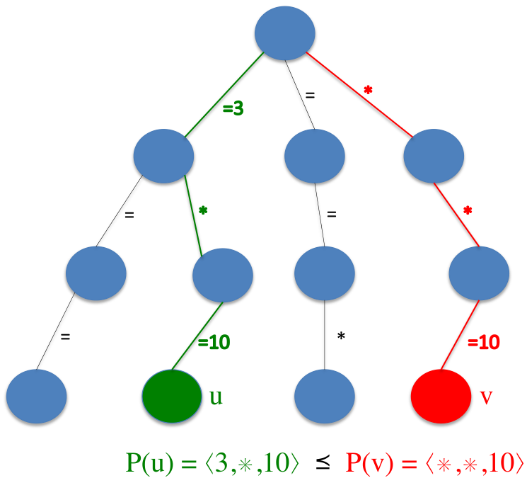
The meaning of the terms “specialization” and “generalization” are as follows. Suppose is a specialization of . Then, the constraints stored in are of “higher-order” than the constraints stored in . To be more concrete, suppose and . Then, for a tuple to satisfy a constraint stored in , it must be the case that , , and belongs to some interval stored in . On the other hand, for the tuple to satisfy we only need and .
F.1 Proof of Proposition 4.2
Proof.
Let be an arbitrary prefix. Recall that the principal filter is a set of nodes – or equivalently the set of patterns – which are above the pattern in the partial order defined in Section 4.2. In particular, for every pattern in , its equality component comes from one of . It follows that is isomorphic to a sub-poset of the prefix poset , which is a chain by Proposition A.6.
Note the important fact that, strictly speaking, the patterns in might come from constraints inserted from relations, or constraints inserted by the outputs of the join. The constraints corresponding to the outputs of the joins always match every entry in a prefix , hence even though Proposition A.6 only infers that the patterns from input relations form a chain, we can safely conclude that the entire poset is a chain. ∎
F.2 Proof of Lemma 4.3
This section analyzes the overall run-time of Minesweeper for -acyclic queries. Let us first summarize what we know so far. Theorem 3.2 showed that the total runtime of Minesweeper (Algorithm 2) is
where is the total time it takes the constraint data structure. Minesweeper inserts a total of constraints to CDS and issues calls to , where is any certificate, is the output size, and is the maximum arity over all relations. What we will prove in this section is, provided that the global attribute order is the nested elimination order, we have
This means the overall runtime is . Hence, in terms of data complexity the runtime is nearly optimal: .
Lemma F.1 (Re-statement of Lemma 4.3).
Suppose the input query is -acyclic, and the global attribute order is a nested elimination order, then each of the two operations and of ConstraintTree takes amortized time , where is the total number of constraints ever inserted into ConstraintTree.
Proof.
For each node , let denote the number of equality components in the pattern . For example, if then ; and if then . Note that , for all .
Our proof strategy is as follows. We equip each of the InsConstraint and getProbePoint operations with “credits.” We then show that those credits are sufficient to account for the runtime of each operation, and at the same time maintain the following interval-credit invariant.
Interval credit invariant: for every node , and for every interval in the list , there is always a reserve of at least credits at any point in time, where is a constant to be specified later. (Note that, by definition, if then the intervals in do not need any reserve credits to maintain the invariant.)
First, for the InsConstraint operation, the interval-credit invariant is easy to maintain. From Proposition 3.1, credits per operation is already sufficient; furthermore, we have up to credits to spend. Hence, we have more than enough to give credits to the interval of the new constraint for a large enough constant . In fact, we will be very generous by assigning credits as follows.
- •
We give the interval component of the newly inserted constraint credits to maintain the interval-credit invariant. Note that for any node in the tree.
- •
We give each component (equality or wildcard) that comes before the interval component of the new constraint credits. How these credits will be used is explained below.
Overall, each InsConstraint operation requires at most
credits as desired. Note again that credits is a lot more than what is required for the InsConstraint operation by itself. We need the extra credit to pay for something else down the line.
Next, we consider a getProbePoint operation. We iterate through the depth of the CDS, for goes from (the root) to (a leaf). At each depth , we try to compute the value , backtracking if necessary. The crucial observation is the following: at each depth of the algorithm, thanks to Proposition A.6, the set forms a totally ordered set because the global attribute order is a nested elimination order. Note that Proposition A.6 only considers input relations. In the constraint tree there might be constraints inserted due to the output tuples. However, those constraints are always the most specific (i.e. they are at the bottom of any poset they participate in), and thus in any poset at any depth the pattern coming from an output-initiated constraint is a specialization of any input-initiated pattern. Furthermore, and this is a slightly subtle point, there are also intervals inserted due to backtracking; but luckily due to the chain property of the prefix poset , for -acyclic queries the backtracking intervals have patterns which are just the same as the patterns from input-generated intervals. Since is a totally ordered set, it has a bottom element .
The basic idea is to show that at each depth the algorithm takes -amortized time, accounted for by using newly infused credits from getProbePoint and the reserved credits from existing intervals guaranteed by the invariant. At the same time, we need to still maintain the interval credit invariant and thus we cannot abuse the banked reserve of the data structure. In particular, intervals whose reserved credits have been used up have to somehow “disappear” or be infused with fresh credits to maintain the invariant.
Specifically, we will equip the getProbePoint exactly credits, distributing precisely credits to each depth of the tree. These credits will be called the depth- credits of getProbePoint.
Fix an iteration at depth of the CDS. If (line 7 of Algorithm 3), then we move on to the next depth and hence depth- credits of getProbePoint is more than sufficient to spend here, assuming is sufficiently large. Henceforth, suppose . Note that we are still considering depth .
Case 1. Let us first assume that there is no backtracking at this depth. Let be the members of the poset , which as explained above is a total order. We will show by induction the following claim.
Claim. For every , the call takes amortized time
while maintaining the interval credit invariant. In other words, we need to use credits from somewhere to pay for this call.
From the claim, and from the fact that
the initial call (line 12 of Algorithm 3) takes time at most . Consequently, the depth- credits of getProbePoint is sufficient to pay for the call.
We next prove the claim by induction. The base case is when , i.e. when we are calling . Line 6 of Algorithm 4 takes -time, thanks to Proposition E.3. Note that,
Hence, with large we have enough credits to pay for the call.
Next, consider and assume the claim holds for . Consider a call to . An iteration of Algorithm 4 has two steps: (a) line 12 takes -credits by the claim’s induction hypothesis, and (b) line 14 takes -time for large. In total, each iteration takes time at most
If we had to continue on with the next iteration (), then it must be the case that for some interval . By the interval credit invariant, this interval has a credit reserve of , which by the above inequality is sufficient to pay for the next iteration! This process repeats itself.
Consequently, the reserves of credits at -intervals that hits pay for subsequent iterations. We are left to pay for the first iteration, the insertion of the new interval in line 17, and fresh credits to deposit to the newly inserted interval to maintain the invariant. It is crucial to notice that the newly inserted interval “consumes” all intervals whose credits we have used up to pay for subsequent iterations. Hence, by paying for , , and above we are done.
With large , the insertion in line 17 takes time at most . Hence, the missing amount in all these three unpaid operations is at most
This proves the claim. Figure 5 illustrates the induction reasoning and where all the credits go.

Case 2. Next, we consider the case when there is some backtracking. When backtracking occurs in line 17, we have credits for each of the components of the constraint from to . We will use these credits as follows.
- •
credits of is used for the insertion in line 17 itself,
- •
credits of is now considered fresh depth- credits of the getProbePoint operation.
- •
credits of for every from to are now considered fresh depth- credits of getProbePoint. We need these fresh credits because the depth- credits from getProbePoint have been used up when we visited depth up to before this backtracking step. Luckily when we backtrack we will never visit the points again due to the constraint inserted in line 17, and hence their credits can be used freely.
∎
F.3 Proof of Proposition 2.8
To prove Proposition 2.8 we need an auxiliary lemma.
Lemma F.2 ([44]).
If -SUM problem does not have a sub-quadratic algorithm, then for every , there exist -partite graphs such that listing all -cycles in needs to take time for any . Further, the graph can be written as where can be written as the disjoint union of edge sets .
Proof.
The result for appears in [44]. The extension to the case of is simple: pick any two partitions and replace each edge (between the two partitions) by a path of length . Note that the resulting graph is -partite (with the claimed special structure on the edge set), has edges and has a -cycle if and only if the original tri-partite graph has a triangle. ∎
Proof of Proposition 2.8.
Consider an arbitrary -cyclic query (with attribute set and relations/hyperedges ). Note that this implies that has a -cycle of length . W.l.o.g. assume that the cycle involves relations and the attributes . In other words, for every , and . The idea is to embed the hard instance for listing -cycles from Lemma F.2 into this cycle. Details follow.
Define
Let be the hard instance for listing -cycles from Lemma F.2, where is the disjoint union of . Further, define the instance for as follows:
Note that the size of the output of in the instance above is exactly the same as the size of the output of . Further, there is a one-to-one correspondence between an output tuple of (and hence ) and a -cycle of . (Indeed for each -cycle in (where ), the output tuple of assigns to attribute for every and every other attribute is assigned .)
Since the relations for are of size , Proposition 2.6 implies that the optimal certificate for has size . We claim that such a certificate can be extended to a certificate for also of size as we did in the proof of Proposition 5.2. Indeed, the certificate for is enough to pinpoint which tuples are the output tuples with comparisons (or certify that the join is empty). Then more comparisons can verify whether each of the output tuples of can be extended to an output tuple of . (The formal argument is pretty much the same as the argument for the proof of Proposition 5.2. The only difference is that can have attributes that are not in and for such attributes we have to check that they have the same values in the projections to for appropriate but this can be done in the claimed time.) Since has -cycles, this will produce an sized certificate for . Thus, an time algorithm to solve for any would (by Lemma F.2) imply a sub-quadratic time algorithm for SUM, which is a contradiction. ∎
Appendix G General queries
In this section, we show that Minesweeper runs in time roughly for general queries (-acyclic or not) where is the elimination width of the GAO. In particular, if the query has treewidth , then there exists a GAO for which the above runtime holds, thanks to Proposition A.7.
The algorithm for general query is the same as that of the -acyclic case; the only (slight) difference is in getProbePoint, which is described next.
G.1 Algorithms
The getProbePoint algorithm for general queries remains very similar in structure to that of the -acyclic case (Algorithm 3), and if the input query is -acyclic with the nested elimination order as the global attribute order, then the general getProbePoint algorithm is exactly Algorithm 3. The new issue we have to deal with lies in the fact that the poset at each depth is not necessarily a chain. Our solution shown in Algorithm 6 is very simple and quite natural: we mimic the behavior of Algorithm 3 on a “shadow” of that is a chain and make use of both the algorithm and the analysis for the -acyclic case.
The “shadow” of is constructed as follows. Let be an arbitrary linearization of nodes in , i.e. if , then either or and are incomparable using the relation . A linearization always exists because is a partial order. Now, for , define the patterns
Here denotes “meet” under the partial order . Then, obviously the shadow patterns form a chain:
Note that it is possible for for . For example, suppose the patterns of nodes in are
and suppose we pick the following linearization of these patterns:
Then, the patterns are as follows.
It should be apparent from the above example the two claims we made earlier: the shadow patterns form a chain, and some shadow patterns are the same. To continue with the above example, getProbePoint is supposed to return a free value on attribute which does not belong to any interval in the interval lists of the nodes
For each node , we will operate as if its pattern was actually . Algorithm 6 has the details.
G.2 Proof of Theorem 5.1
Proof.
Let us first go through the skeleton of Algorithm 6. We encourage the reader to view Algorithm 3 and Algorithm 6 side-by-side. Their structures are identical except in two places. First, lines 12 to 17 of Algorithm 6 build a shadow chain because itself is not necessarily a chain as is the case in Algorithm 3. Second, the call to nextChainVal on line 12 in Algorithm 3 is replaced by the call on line 20 of Algorithm 6 to nextShadowChainVal.
For the moment, suppose the calls to nextChainVal and nextShadowChainVal take the same amount of time, then the only extra work that Algorithm 6 does compared to Algorithm 3 per depth of the CDS comes from building up the shadow poset. It takes time for each shadow poset. (Recall that is the number of intervals ever inserted into CDS by Minesweeper.) And, if we also want to maintain the interval credit invariant then it takes -time extra per depth per getProbePoint operation. Up to this point, we can mimic the proof from the -acyclic case and assign each getProbePoint operation credits. The only difference (so far) from the analysis of the -acyclic case is that the amount of credits per depth assigned to getProbePoint is blown up by a factor of due to the shadow poset construction and the extra credits needed for the shadow intervals. Note also that, modulo the difference between the nextChainVal call and the nextShadowChainVal call, if the poset is a chain, then is exactly and every node is a shadow of itself! In this case, we do not need to do the extra work of building up the shadow poset and indeed we “get back” Algorithm 3.
Next, let us look at Algorithm 4 and Algorithm 7 side by side. The key difference is in the calls to Next on an interval list, we make a call to nextChainVal on the chain , where is the shadow of . (Since is the meet of all nodes from and above in the linearization, and hence is a chain.) If we maintain the interval credit invariant, then each of these calls to takes amortized time , a -blowup compared to Next. So far, we have an blowup factor (with a very loose analysis), relative to the -acyclic case.
Note again that, if the poset is a chain, implying , and every node is a shadow of itself, then the calls to and to are identical. In this case nextShadowChainVal is the same as nextChainVal and we get back to the -acyclic case.
In general, however, we cannot maintain the interval credit invariant by simply giving each inserted interval credits (blown up by more) as we have done in the -acyclic case because the same node might have different shadows depending on the prefix we are working on. For example, the node might have the shadows , , , and so forth. In this example, the number of credits we give to an interval in the list has to be at least three times as much as that in the -acyclic case because might participate in the nextChainVal calls with each of its shadows. Consequently, we will have to give each inserted interval many more credits than . The key question is: how many more credits?
The number of credits assigned to each interval depends on the size of its pattern, and on what type of interval it is. From Theorem 3.2, we know that the number of intervals inserted into the CDS is . In fact, there are two types of intervals inserted: intervals inserted by the output called the output-generated intervals, and intervals inserted by the input relations, called the input-generated intervals. There are also backtracking intervals created by the algorithm. Hence, overall we have three types of intervals.
The overall credit-assignment scheme is intimately tied to the size of interval pattern under consideration. Recall that the size of a pattern is defined to be the number of equality components of the pattern. For example, the pattern has size and the pattern has size .
Consider the simplest case when has size , such as . In this case, the node is always on top of the linearization and thus in it is the shadow of itself. In other words, it does not really have any shadow. The symmetric situation is when has no wildcard pattern. All of the intervals that come from the outputs are of this type. This includes backtracking intervals which are created from a prefix of output-generated intervals. In this case, is always at the bottom of the linearization and thus in it is also a shadow of itself. For these types of intervals – intervals in where is self-shadowed – we can give them the same credits as they get in the -acyclic case (multiplied by the blowup factor).
Next, we analyze how many credits we need for intervals whose patterns are not self-shadowed at some point in the execution of Minesweeper. (A pattern might be self-shadowed at one point, but then not self-shadowed at another time due to a different prefix.) Let be one such pattern with size ; let be the length of the pattern , i.e. intervals of are on attribute in the global attribute order. Then, the support of (the positions of equality components) is precisely a subset of the universe of the prefix poset as defined in Section A.2. From Proposition A.7 we know that , and hence . (If then is self-shadowed.) Since out of components in are already fixed, the number of different shadows of is at most : it has degrees of freedom, each of which can be attributed to some interval in the set of input-generated intervals. Consequently, we can give each interval in the following number of credits to pay for all operations it’s involved in: . In the above accounting we did not need to distinguish between input-generated intervals or backtracking intervals, namely can be the prefix of a backtracking interval too.
Let us summarize what we know thus far:
- •
Intervals whose patterns are self-shadowed get the same credits as in the -acyclic case.
- •
Other intervals with size- patterns get credits.
(Again, the credits are supposed to be multiplied by .) So our next task is to sum up all the credits we need and that will be the final (amortized) runtime of Minesweeper.
- •
Each output-generated interval gets credits. (We already multiplied in the blowup factor.) The total contribution of output-generated intervals to the overall runtime is thus .
- •
Each input-generated interval with pattern of size gets credits. Each input-generated interval with pattern of size receives
credits. Since there were at most input-generated intervals, the total number of credits infused is at most
- •
Lastly, we account for the backtracking intervals whose patterns are not self-shadowed. The number of such intervals with a size- pattern can be upperbounded by , because every backtracking interval must have come from a pattern (of size ) and each equality component of the pattern can be attributed to an input-generated interval. Each such interval, as analyzed above, gets credits. Hence, overall we need
Overall, over-estimating by a lot, we need to pump in
To get the last inequality, we bound – the number of intervals ever inserted in to the CDS – as follows. is at most the number of input-generated intervals plus the number of output generated intervals plus the number of backtracking intervals:
∎
G.3 Proof of Proposition 5.2
Proof.
We prove this result by using the reduction from unique-clique to the natural join evaluation problem. The unique--clique input instance ensures that the output size is at most . Let’s say the input graph is (with no self loops), which is guaranteed to either have no clique or exactly one clique. Then consider the following query
where the domain of each for is ,
and . Note that is empty if has no clique otherwise has exactly tuples (corresponding to each of the assignments of the vertices of the clique in to ). Further, is -acyclic because of the presence of . Finally, it is easy to verify that has treewidth .
Next, we argue that the certificate size of the query above is . To see this, first consider the sub-query
Since all the relations are of size , Proposition 2.6 implies that the optimal certificate for has size . We claim that such a certificate can be extended to a certificate for also of size . Indeed, the certificate for is enough to pinpoint which tuples are the output tuples with comparisons (or certify that the join is empty). Then more comparisons can verify whether each of the tuples is in or not. This will produce an sized certificate for .1313 13 More formally, let and define . Further, let for . Then to “pinpoint” whether , we run the following binary searches: for , perform binary search to compute a such that . Then perform the binary search to compute such that . If any of the ’s do not exist, then is not in otherwise it does. It is easy to check that the above set of comparisons (along with the comparisons in the certificate for ) constitute a valid certificate for (in the sense of Definition 2.3). Finally, note that each binary search can be done with comparisons, which implies the claimed certificate size of . Thus, if there were an algorithm for , it would determine if has a clique or not in time .
However, Chen et al. [18] showed that if there was an -time algorithm solving unique--clique, then the exponential time hypothesis is wrong, and many -complete problems have sub-exponential running time. This implies that for large enough , the above time algorithm will be a contradiction. ∎
G.4 Proof of Proposition 5.3
Proof.
We will in fact prove this result using the same query family as in Proposition 5.2. In particular, we define
As was observed in the proof of Proposition 5.2, is both -acyclic and has treewidth .
W.l.o.g. assume that the global attribute order is . Now consider the following input instance:
and
It is easy to check that the output of on the input above is empty and that . To see why the latter is true note that with equalities one can certify for every . Further with further equalities and one comparison one can certify that the output is empty. Thus, we need overall comparisons. To complete the proof, we will show that Minesweeper on the input above runs in time , which would prove the result (since we are ignoring the query complexity). In fact, we will prove this claim by showing that Line 20 in Algorithm 6 is executed times.
For simplicity, we will assume that Minesweeper always has the interval inserted in all branches of its CDS.
We will argue Minesweeper has to consider all possible prefixes of size : . In particular, for each such prefix Algorithm 6 executes Line 20. One can show (e.g. by induction) that for any such prefix , the only constraints in the CDS that can rule them out are of the form for and . However, this implies that to rule this prefix (specifically the potential tuple ) out, Algorithm 6 has to “merge" at least two of these constraints, which means that Line 20 has to be executed at least once1414 14 Note that all the constraints listed above might not exist in which case Line 20 might not be able to rule the tuple out but that is fine since the outer algorithm will rule this tuple out., as desired. ∎
Appendix H end-to-end results for the set intersection query
This section describes our results specialized to intersection queries, which have been discussed by previous work. The purpose is for the interested reader to both see all the tools used in this simple example and be able to more directly compare our results with previous results on set intersection. Also, this query and the bowtie query in the next section are both -acyclic (with any GAO); these two sections illustrate many of the key ideas in our outer algorithm analysis, the design and analysis of CDS and getProbePoint, without too much abstraction.
H.1 The set intersection query
Definition H.1 (Set intersection query).
The set intersection query is defined as
In this query, each input relation is unary over the same attribute . So each input relation can be viewed as a set of (distinct) values over the domain . The output is simply the intersection of all input relations . In this case, , , for all , and an output “tuple” is a one-dimensional vector of the form , where .
In this section, we present Minesweeper specialized to the intersection query . To recap, consider the following problem. We want to compute the intersection of sets . Let . We assume that the sets are sorted, i.e.
The set elements belong to the same domain , which is a totally ordered domain. Without loss of generality, we will assume that .
In “practice” it might be convenient to think of as the index set to another data structure that stores the real domain values. For example, suppose the domain values are strings and there are only strings this, is, interesting in the domain. Then, we can assume that those strings are stored in a -element array, and the value is one of the three indices into the array.
H.2 The CDS for
The CDS for is a data structure that stores a collection of open intervals of the form , where and are in the set . When two intervals overlap they are automatically merged. We overload notation and refer to both the data structure and the set of intervals stored as CDS. The data structure supports two operations: InsConstraint and getProbePoint.
- •
The InsConstraint operation takes an open interval and inserts it into the CDS.
- •
The getProbePoint operation either returns an integer that does not belong to any stored interval, or returns null if no such exists.
- •
If CDS is empty, then returns an arbitrary integer. We use as the default.
Two options for implementing the constraint data structure CDS
If we implement the data structure CDS straightforwardly, then we can do the following. We give each input interval one credit, to each end of the interval. When two intervals are merged, say is merged with to become , we use credit from and credit from to pay for the merge operation. If an interval is contained in another interval, only the larger interval is retained in the data structure. By maintaining the intervals in sorted order, in -time the data structure can either return a probe point that does not belong to any stored interval, or correctly report (return null) that no such exists. In other words, each call to getProbePoint takes amortized constant time. Inserting a new interval into CDS takes -amortized time where is the maximum number of intervals ever inserted into CDS, using the credit scheme described above.
On the other hand, if we apply the strategy of always returning the least value of that does not belong to any stored interval, then it is easy to see that CDS essentially only needs to maintain one interval . Initially when CDS is empty is returned. After that – referring forward to the outer algorithm presented in the next section – the newly inserted intervals always contain and the new single interval maintained in CDS becomes for some . Insertion of a new interval only takes constant time because we only need to compare the high-end of the interval with the current value. In this case, the algorithm becomes the minimum-comparison method in [20] and it is the same as a typical -way merge join algorithm.
H.3 The outer algorithm for intersection
The outer algorithm for Minesweeper specialized to evaluate is presented in Algorithm 8. In this case, each constraint is an open interval of the form , where and are integers. An interval is inserted into the constraint data structure CDS if the algorithm has determined that the interval contains no output. Note that and/or themselves might be part of the output, but any value in between is not. In particular, the constraint data structure CDS stores a set of constraints and thus we will use the term constraint set to refer to the set of intervals stored in CDS.
We next run through the elements of the argument and the algorithm for the case of .
H.4 Analysis
We specialize notions of argument and certificate to in order to illustrate these concepts.
Definition H.2 (Argument for ).
An argument is a finite set of symbolic equalities and inequalities, or comparisons, of the following forms: (1) or (2) for and . An instance satisfies an argument if all the comparisons in the argument hold for that instance.
Definition H.3 (Certificate for ).
An argument is called a certificate if any collection of input sets satisfying must have the “same” output, in the following sense. Let be an arbitrary set of unary relations such that , for all , and that satisfy all comparisons in the certificate , then the following must hold:
if and only if
The tuple is called a witness for this instance of the query. Another way to state the definition is that, an argument is a certificate iff all instances satisfying the argument must have the same set of witnesses.
The size of a certificate is the number of comparisons in it. The optimal certificate for an input instance is the smallest-size certificate that the instance satisfies. The optimal certificate size measures the information-theoretic lowerbound on the number of comparisons that any comparison-based join algorithm has to discover. Hence, if there was an algorithm that runs in linear time in the optimal certificate size, then that algorithm would be instance-optimal.
The following theorem along with Proposition 2.5 imply that Algorithm 8 has a near instance-optimal run-time. up to an factor. Since is part of the query size and the output has to be reported, Minesweeper is instance-optimal in terms of data complexity up to a factor for this query.
Theorem H.4 (Minesweeper is near instance optimal for ).
Algorithm 8 runs in time , where is any certificate for the instance, is the input size, and is the output size.
Proof.
We show that the number of iterations of Algorithm 8 is , and that each iteration takes time .
To upperbound the number of iterations, the key idea is to “charge” each iteration of the main while loop to either a distinct output value or a pair of comparisons in the certificate such that no comparison will ever be charged more than a constant number of times. Each iteration in the loop is represented by a distinct probe value . Hence, we will find an output value or a pair of comparisons to “pay” for instead of paying for the iteration itself.
Let be a probe value in an arbitrary iteration of Algorithm 8. Let and be defined as in lines 7 and 8 of the algorithm.
First, consider the case when for all , i.e. is an output value. Note that in this case for all . We pay for by charging the output . The new constraint inserted in line 11 ensures that we will never charge an output twice.
Second, suppose for some , i.e. is not an output. (Note that by definition it follows that .) For each , the variable is said to be -alignable if is already equal to (in which case ) or if is not part of any comparison () in the certificate . Similarly, we define the notion of -alignability for , .
When is -alignable, setting will not violate any of the comparisons in the certificate . Similarly, we can transform the input instance to another input instance satisfying by setting , provided is -alignable.
Claim: if is not an output, then there must exist some for which both and are not -alignable. In particular, in that case
and both and are involved in comparisons in the certificate.
Before proving the claim, let us assume it is true and finish off the charging argument. We will pay for using any comparison involving and any comparison involving . Because they are not -alignable, each of them must be part of some comparison in . Since we added the interval to the constraint data structure CDS, in later iterations will never hit the same interval again. Each comparison involving one variable will be charged at most times: one from below the variable, one from the above the variable, and perhaps one when the variable is output.
Proof of claim. Suppose to the contrary that at least one member of every pair and , , is -alignable. Let such that is -alignable, . Let be such that . The value must exist because is not an output. First, by assigning for all , we obtain an instance satisfying the certificate for which
| (6) |
Second, by assigning for all , we obtain an instance also satisfying the certificate for which (6) does not hold! This contradicts the certificate definition; hence, the claim holds.
We have already discussed how the constraint data structure CDS can be implemented so that insertion takes amortized constant time in the number of intervals inserted, and querying (for a new probe point ) takes constant time. Given a probe point , searching for the values and takes -time, for each . Hence, each iteration of the algorithm takes time at most . ∎
Remark H.5.
In fact, if we implement Minesweeper using the galloping/leapfrogging strategy shown in [20] and [53], then we can speed up the search for the values and of Algorithm 2 slightly in terms of asymptotic runtime. Those ideas in fact work very well in practice! However, they are regarded as “implementation details” in this paper and will not be discussed further. We are happy with a -factor loss.
Appendix I End-to-end results for the bowtie query
To illustrate the key ideas of the analysis of Minesweeper, we present in this section the second end-to-end set of results on a query that is slightly more complex than the intersection query from Section H. The hope is, without burdening the reader with the heavy notation from the general algorithm, the so-called bowtie query is able to illustrate many key ideas. We will define what the query is, what are arguments and certificates for this query, what are the constraints and the CDS, the outer algorithm, and finally the analysis. It turns out that the CDS for this query is very simple. Additionally, the bowtie query is -acyclic, and any GAO is a nested elimination order!
I.1 The bowtie query, arguments, and certificates
Definition I.1 (Bow-tie query).
The bow-tie query is defined as
In this case, , , and a tuple is in the output if and only if , , and .
Due to symmetry, the global attribute order (GAO), without loss of generality, can be assumed to be . The relations , , and are assumed to be already indexed, allowing for the following kind of access.
- •
is the set of all values in .
- •
is the th smallest value in , where is the index and the value belongs to the domain of attribute .
- •
Similarly, , and is the th value in .
- •
is the set of all -values in
- •
is the th smallest -value in
- •
is the set of all -values among tuples with .
- •
is the th -value among all tuples with .
In the above, when we say th smallest value we use the set semantic. There is no duplicate value and thus no need to break ties. We next specialize notions of argument and certificate to this particular query in order to illustrate these concepts.
Definition I.2 (Argument for ).
An argument for the bow-tie query is a set of comparisons in one of the following three formats:
where is called a comparison.
Since the -values in and -values in are distinct, there was no need to allow for comparisons between tuples in or between tuples in . Allowing for such comparisons does not change our analysis.
Definition I.3 (Certificate for ).
For the bow-tie query, an argument is called a certificate if the following conditions hold. Let be three arbitrary relations such that
and that the and satisfy all the comparisons in . Then, for any triple ,
if and only if
Such a triple is called a witness for the instance ; and, it is also a witness for the instance .
Following the lead from Example B.3, it is not hard to construct an example showing that comparisons between -variables between tuples in are sometimes crucial to reduce the overall certificate size.
I.2 Constraints and the CDS
For the bow-tie query every constraint is of one of the following three forms:
- •
,
- •
,
- •
or .
where , .
A tuple satisfies the constraint if ; it satisfies the constraint if and ; and it satisfies the constraint if .
Each constraint can be thought of as an “interval” in the following sense. The first form of constraints consists of all two-dimensional (integer) points whose -values are between and . We think of this region as a 2D-interval (a vertical strip). Similarly, the second form of constraints is a 1D-interval, and the third form of constraints is a 2D-interval (a horizontal strip).
We store these constraints using a two-level tree data structure (which is a ConstraintTree specialized to the two attribute case). Figure 6 illustrates the data structure.

In the first level (the root node), there is a collection of intervals indicating the ruled out -values. Then there are branches to the second level. Each branch is marked with an , or for some integer that does not belong to any interval stored at the root.
In the second level of the tree, every node has a collection of open intervals. Intervals belonging to the same node are merged when they overlap. So, the collection of intervals at each node are disjoint too. To analyze the cost of merging we use a credit based argument. Every inserted interval is given one credit. We use the trick of giving the low end and the high end of an interval half a credit to pay for the merging of two intervals. If the second level of a -branch covers the entire domain, then the -branch is turned into a constraint that can further be merged (at the root level). Effectively, the interval is inserted into the interval list of the root node. We will give an extra credit to the -branch so that when the branch is turned into a interval both of the end points has half a credit as any other interval of the root.
Inserting a new constraint takes amortized logarithmic time, as we keep the branches sorted, and the new constraint might “consume” existing intervals. (This logarithmic factor can be improved to constant time if the Minesweeper algorithm and the constraint data structure work in concert, but we will not dig deeper into this detail at this point. We rather keep the description generic, and separate as much as possible the inner workings of the algorithm from the data structure.) In amortized constant time, the data structure CDS is able to report a new tuple that does not satisfy any of its constraints, or correctly report that no such exists. To find , we apply the following strategy:
- •
We first find such that does not belong to any root-level interval. This value of , if it exists, can easily be found in constant time by taking the right end point of the lowest interval from the interval list at the root. (Recall the invariant that intervals are disjoint!). If there is no first level interval, then we can set
- •
If is found and there is no branch, then we find a value that does not belong to any second level interval on the -branch. If there is no branch, then set . If no exists then no such exists, the algorithm terminates.
- •
If is a first-level branch, we find a value under the -branch that does not belong to any interval under that branch. We call such a a “free value” . The tuple might still violate a constraint in the -branch. In that case, we insert the constraint into the tree. Then we find the next smallest “free” value under the -branch again and continue with the “ping-pong” with the -branch until a good value of is found. The intervals under -branch might be merged with an interval taken from the -branch, but if we give each constraint a constant number of credits, we can pay for all the merging operations.
To summarize, insertion and querying for a new probe point into the above data structure takes at most logarithmic time in the amortized sense (over all operations performed).
I.3 The outer algorithm
We next describe the outer algorithm of Minesweeper specialized to the bowtie query. The key of Algorithm 9 is the loop. We begin with a point that has not been ruled out by the constraint data structure at this point of the algorithm. Intuitively, our goal is to determine if is in the output; if it is not in the output, then our goal is to find some gap that could rule out . We find the gaps by probing each of the relations , , and “around” the point .
The probes of and are straightforward: we find gaps around the value of and in each relation. With respect to , if we only needed to verify that is not an output tuple then a gap around the value in would suffice. However, we do a bit more work in Lines 9 to 11; the reason for that is explained below. Before then, observe that if is in the output then (in fact, for all ). Thus, the condition in Line 12 is a sound and complete check for to be in the output.
 |
 |
|---|---|
| (a) | (b) |
As we noted, Minesweeper does more work than is necessary to certify that is not an output tuple. This is because Minesweeper is not only searching for a gap that contains to rule out, but it also “looks for” a variable that is involved in any certificate (including the optimal certificate); this is done so that the algorithm does not explore too deep into – and thus spend too much time in – regions that the optimal certificate wastes very few comparisons to rule out. At the same time, we also have to ensure that we don’t explore too many gaps just to capture one single comparison in the optimal certificate. Minesweeper steps on this fine line roughly as follows.
Since could have been excluded by a gap that does not have on its boundary, Minesweeper– analogously to the eponymous windows game when one chooses a square without a bomb (see Figure 7) – finds the biggest gaps around the point . In this case, we observe that for each , Minesweeper examines a constant number of gaps. From Lines 15 onward, we simply insert all the gaps that we found above. Later, we will reason that some comparison in any optimal certificate is found by at least one of the FindGap searches. In this example, we explored a constant number of gaps (here ) for every ; for more complex queries, the number of gaps may grow, but it will grow with the number of attributes in , i.e., the number of gaps we explore does not depend on the data.
Algorithm 9 presents the formal details of the algorithm. Notations are redefined here for completeness. Let denote the number of tuples in the corresponding relations, the set of -values in , the ’th -value, the set of ’s for which , and the ’th -value in the set .
Figure 8 illustrates the choices of various parameters in the algorithm. Some of the constraints might look unintuitive and perhaps redundant at first. The picture shown in Figure 8 should give the reader the correct geometric intuition behind the constraints: all points in satisfying the constraints are guaranteed to be not part of the output.

To convey the subtlety in gap exploration, let us consider a simple idea. The first candidate gap from that comes to mind is perhaps the gap between and where is the largest tuple in that is smaller than lexicographically, and is the smallest tuple in that is greater than lexicographically. The problem with this simple idea is that this gap might actually fail to capture any variable involved in an optimal certificate comparison at all. Consider, for example, the following input:
The certificate is an optimal certificate for this instance. Suppose the probe point is , then and both of which do not have anything to do with the optimal certificate above.
I.4 Analysis
We next show Algorithm 9 is near instance optimal (modulo the time spent in the CDS). This Theorem parallels the content of Theorem 3.2 so the reader can map back this special case to the general statement.
Theorem I.4 (runtime of Minesweeper on ).
Let denote the total number of tuples from the input relations, the total number of output tuples. Let be an arbitrary certificate for the input query. Then, the total runtime of Algorithm 9 is
where is the total time it takes the constraint data structure. The algorithm inserts a total of constraints to CDS and issues calls to getProbePoint.
Proof.
We show that the number of iterations of Algorithm 9 is . Since the amount of work done in each iteration is and the number of calls to and the number of inserted constraints are linear in the number of iterations, the proof is complete.
We “pay” for each iteration of the algorithm, represented by the tuple that the CDS returns in the while predicate for that iteration, by “charging” either an output tuple or a pair of comparisons in the certificate . We show that each output tuple and each comparison will be charged at most times. To this end, we define a couple of terms.
Any variable
is said to be -alignable if either is already equal to or is not involved in any comparison in the certificate . By convention, any variable whose index is out of range is not -alignable. The semantic of -alignability is as follows. If a -alignable variable is not already equal to , setting will transform the input into another database instance satisfying all comparisons in without violating the relative order in the relation that belongs to.
A variable
is said to be -alignable if either is already equal to or is not involved in any comparison in the certificate . A variable
is -alignable if is -alignable and either is already equal to or is not part of any comparison in the certificate . Similarly, we define -alignability for a variable
Next, we describe how to “pay” for the tuple .
Case 1
Case 2
The else part (line 15) is executed, i.e. is not an output tuple. We claim that one of the following five cases must hold:
- (1)
both and are not -alignable,
- (2)
both and are not -alignable,
- (3)
both and are not -alignable,
- (4)
both and are not -alignable,
- (5)
both and are not -alignable.
Suppose otherwise that at least one member in each of the five pairs above is -alignable. For example, suppose the following variables are -alignable:
Then, we construct two database instances as follows.
- •
Database instance . In this instance, we keep all current variable values except that we set and . Then, clearly in this instance the set of index tuples is a witness for .
- •
Database instance . This instance requires a little bit more care. Recall that we are in the case when is not an output tuple. Hence, it cannot possibly be the case that and already. Assume, for example, that . Then, the database instance is constructed by setting and . Then, in this case is not a witness for .
Note that both and satisfy . Hence, we reach a contradiction because is a certificate. The claim is thus proved.
The key idea is, by definition each non-out-of-range variable that is not -alignable must be involved in a comparison in the certificate . There is an exception, something like might be non--alignable because its prefix variable is not alignable. But in that case must be involved in a comparison in the certificate, and that’s all we need for the reasoning below.
Instead of charging a comparison, we will charge a non-out-of-range non--alignable variable. If each non-out-of-range non--alignable variable is charged times, then each comparison will be charged -times.
We pay for by charging any pair of non-out-of-range non--alignable variables out of the five pairs above that are involved in comparisons in . We call each of those five pairs an “interval." The pairs of the type (1), (2), and (5) are 2D-intervals, and the pairs of the type (3), (4) are 1D-intervals.
Due to the constraints added on lines 18, 20, and 22, the 2D-intervals are charged at most once. Since two 2D-intervals might share an end point, each non-out-of-range non--alignable variable from a 2D-interval might be charged twice. The 1D-intervals are charged at most twice. Each non-out-of-range non--alignable variable from a 1D-interval might be charged at most four times. Consequently, each comparison is charged times. ∎
Appendix J Counter examples
In this section, we present a family of -acyclic join queries and instances on which none of Leapfrog-Triejoin [53] (LFTJ henceforth), the algorithm of [40] (NPRR henceforth) or Yannakakis’ algorithm [55] are instance optimal (i.e. they don’t run in -time). Furthermore, the gap between those algorithms and Minesweeper can be arbitrarily large.
To simplify the argument, let us first consider a simpler family of instances. The query is the following.
The above query is -acyclic, and the GAO is a nested elimination order. The main idea behind the instance is to “hide" the certificate along a long path in the query. All three algorithms NPRR, LFTJ, and Yannakakis do not explore the attributes globally as Minesweeper does, and hence they will get stuck looking for many partial tuples that do not contribute to the output.
The relations are constructed as follows. Each attribute will have as its domain the set , where and is a large positive integer. Each relation will have “chunks,” where the th chunk () is a subset of the set
More precisely, relation is defined as follows.
- •
For every , the th chunk of is exactly exactly
- •
The th chunk consists of one single tuple .
- •
And the ’th chunk is empty.
If , then we interpret as . Namely, the th chunk of is empty. Note that every relation is of size .
It is not hard to see that the output of the above instance is empty. Furthermore, there is a certificate of size . Hence, by Theorem 2.7 Minesweeper takes time since is a nested elimination order.
This certificate consists of the following comparisons
| . . . | . . . | . . . | ||
To see why this is a certificate that the output is empty, consider an arbitrary witness for this instance:
From the first two (sets of) inequalities above, we know . Then, from the next inequality we know . This inference goes on until the last inequality, which does not leave any room for . Hence, such a witness cannot exist.
Now, for every , the semijoin has size . Hence, Yannakakis algorithm runs in time at least .
For LFTJ and NPRR, it takes slightly more work to be rigorous, but the key ideas are as follows. Consider any attribute ordering that LFTJ adopts. Say the attribute ordering is , for some permutation of . LFTJ will compute the intersection on , and for each value in the intersection it will compute the join on using as an anchor, and so on. If , then clearly the runtime is because the intersection on each attribute is . If , then LFTJ will go through every tuple in the input relation after it is semijoin-reduced on and . And even after two such reductions, the size of the relation is still . The algorithm NPRR suffers the same drawback.
There are two potential unsatisfactory aspects of the instance above: (i) The gap between Minesweeper and the worst-case algorithms is only quadratic and (ii) the example only considers path type queries. Next, we handle these two shortcomings.
We can increase the gap in the above example by considering the following join query:
Then, each relation still has blocks like before, where the th block for is . For the block has only one tuple , and the th block is empty. It is not hard to see that there is a certificate of size , and all three algorithms Yannakakis, NPRR, and LFTJ run in time at least . The reasoning is basically identical to the previous example.
Finally, we tackle the class of -acyclic queries for which our quadratic gap holds. We note that our argument holds for any -acyclic query into which we can embed the -path query. In other words, as long as a -acyclic query has attributes and relations such that is only present in and (except for the cases in which case only exists in and the case of in which case only exists in ), we can embed the hard instance above into a hard instance for , where we extend the values for other attributes and relations as we did in the proof of Proposition 2.8 (in Appendix F.3). Recall that the proof in Appendix F.3 shows that this does not change the certificate size (which implies that the runtime of Minesweeper remains the same) while it is not hard to check that the worst-case optimal algorithms still are quadratically slower. We note that we did not try to optimize the length of the shortest path for which our hard instance still works. However, we note that the argument cannot work for path of length (since LFTJ is instance optimal for the query , which is essentially the bowtie query). Note that the class of -acyclic queries that has a -path embedded in it as above is a fairly rich subset of -acyclic queries.
Appendix K Our certificate vs. the notion of proof from DLM.
It is perhaps instructive to compare and contrast our notion of certificate from the similar notion of “proof” from DLM. The obvious difference is that our certificate is defined for a natural join query, while DLM’s “proof” is only defined for the query. The difference, however, is subtler than that. Consider only the case. DLM’s proof is output-specific while our certificate does not need any specific mentioning of the output at all. For some subset of domain values, they defined a -proof to be an argument for which each value is certified with a spanning tree of equalities, and each of the set of values in between consecutive values in must be “emptiness-certified” with an -proof. An -proof in DLM is defined in terms of “eliminating” elements by the comparisons. (See DLM’s Lemmas 2.1 and 2.2 and Theorem 2.1.) Our notion of certificate is stronger. For example, our certificate does not need any comparison to certify that the output is empty. For example, consider intersection of three sets of the same size . An emptiness certificate may consist of two equalities: . It is obvious that any instance satisfying those two inequalities must have an empty intersection because we can infer that . Subtler than that, Example B.3 points to the fact that the use of equalities can asymptotically reduce the certificate size even when the output is empty.
Appendix L The Triangle Query
The goal of this section is to prove Theorem 5.4. We begin with the data structure CDS.
L.1 The CDS
We begin by collecting some properties of a data structure that maintain interval lists that will be useful in our new definition of CDS.
L.1.1 Dyadic Tree for Intervals
Let for ease throughout.
- •
The data structure consists of nodes that contain an interval list. We index the nodes of the tree by binary strings of length less than or equal to , i.e,.
e.g., is the root, is the left child, and while is the rightmost leaf. We can think of string of length as denoting the interval each as a binary expansion of a value, i.e., .
- •
Each node is associated with an interval list on domain denoted .
- •
Given an interval , we will need its dyadic decomposition, i.e., one of the intervals above and we denote it
For any interval, in we have . Let be the string associated with the dyadic interval .
- •
For every dyadic interval node , there is an IntervalList . We also insist that any consecutive interval is stored as the collection . (This makes the upcoming arguments simpler.)
- •
: For each , set
This takes since there are dyadic intervals and insertion into an IntervalList takes time.
- •
for dyadic : Returns the interval list for . This can be done in time, where is the total number of (dyadic) intervals that need to be output. Note that to perform this task one has to find the correct position of and in (which can be done in time) and then returning the corresponding intervals. There are two cases: (i) The output is , in which case we “charge" the intersection to this interval (note that we have in this case) or (ii) The output is a subset of intervals from : in this case we “charge" the intersection to these set of intervals. (Note that we can only have in case (ii).) This charging scheme will be useful in the proof of Proposition L.1 below.
L.1.2 The New CDS
For notational convenience we will denote the interval lists for prefixes and simply as and .
Our new CDS would be very similar to our earlier CDS in Appendix E except in the following way:
The -branch for variable would be replaced by a dyadic tree containing all the intervals of the form . In other words in addition to maintaining the interval lists , it will also maintain for dyadic interval of the interval list , which will always satisfy the following invariant:
| (7) |
Not surprisingly, we will maintain the interval lists as a dyadic tree as outlined in the previous section. For the rest of the argument we will show that the insert operation on the new CDS can be done in amortized time. For all constraints except of the form the insert can be done in amortized time by Proposition 3.1. So we only need to show the following:
Proposition L.1.
Given a dyadic tree on domain with insertions of the form , then (7) can be ensured in time .
Proof.
We use the natural algorithm to implement the insert of constraints of the form , which we outlined next. Let be . Then perform our original . Then do the following for every . Let , where is the sibling of in the dyadic tree. If is empty we stop otherwise we recurse with this algorithm at the parent of (where we want to insert all intervals in into ).
We first assume that the algorithm only deals with dyadic intervals throughout. We claim that under this assumption we would be done by assigning credits to each inserted interval. To see this first consider the simple case, where we always have , i.e. we always need to insert one interval. In this case, for each recursive level we do amounts of work and we have recursive calls (up the path in the dyadic tree from the leaf corresponding to to the root) overall. We expand a bit on the work on each recursive call. Recall that the analysis of the Intersect procedure: we first need work to figure out the correct position of in the IntervalList of . To pay for this we use up credits from . We still have to pay for the computation of . We pay for this by charging or as appropriate. The important point to note that is that once an interval stops “floating" up, it can only be pushed by fresh intervals that arrive at its sibling node at a later point of time.
For the more general case (but still with dyadic interval), note that any interval that “floats" up is either one of the inserted intervals or is “sandwiched" between two such inserted intervals. Adjusting the constant for the number of tokens appropriately takes care of this issue.
Finally to handle the general case, we can replace any interval by dyadic intervals. To deal with this we need to increase the number of credits to from the previous credits. This completes the proof. ∎
Finally, we will also ensure the following:
For every constraint that is inserted into , we also insert into the interval list for every .1515 15 Note that Proposition L.1 only talks about singleton , it can easily be checked to see that it can handle this more general case. Basically we can make all such to be the leaves in the dyadic tree and the argument in Proposition L.1 can handle insertions into leaves.
L.2 The Algorithm
The outer algorithm for will be the same as in Algorithm 2. We will have to change the getProbePoint algorithm, which is formally presented in Algorithm 10.
Algorithm 10 uses the following helper functions:
- •
: Finds the smallest value that is not covered by . We implement this algorithm by the MERGE algorithm.
- •
: Returns the next node in the dyadic tree by the pre-order traversal (returns null if the traversal is done). It is simple to implement: let . Let be the largest index such that . Then return . If no such exists, return null.
- •
We maintain a data structure, which keeps track of the last “uncovered" value considered by the algorithm in the union of and . The function returns this cached value while updates the cached value to .
Further, we will assume that when the outer algorithm outputs a tuple and adds the constraint , there is an accompanying call to .
It is not hard to see that Algorithm 10 is correct. We state this fact without proof:
Lemma L.2.
Algorithm 10 correctly returns a tuple that is not covered by any existing constraints. If no such tuple exists then it correctly outputs null.
Lemma L.3.
Proof.
This follows from the fact that the time spent is in some sense running Algorithm 3 on , which is a -acyclic query. So our earlier proof can be easily adopted to prove the lemma. ∎
Lemma L.4.
Time spent over prefixes that satisfy the condition in Step 17 is upper bounded by .
Proof.
This just follows from the fact that the total time spent is bounded by (up to constants):
as desired. ∎
The next couple of lemmas need the following definition:
Definition L.5.
We first argue that the number of pairs with is bounded:
Lemma L.6.
Proof.
Note that we only need to consider the values for which . Fix such an arbitrary and consider an arbitrary . Now when the Algorithm gets to Step 21 we know the following:
- •
- •
.
- •
All of the above imply that there exists a such that the tuple is not ruled out by the current set of constraints. This implies that Algorithm 10 will return such a tuple (by Lemma L.2). This probe point will then be used by the outer algorithm to either (i) discover a new constraint or (ii) recognize it as an output tuple.
If there is even one such that the returned tuple fall in category (i) above, then note that we can assign a unique inserted constraint to the prefix (among all such prefixes that have such that falls in category (i)). This by the argument for the runtime of the outer algorithm implies that the number of such prefixes is bounded by .
Thus, we only have to consider prefixes such that every tuple returned by Algorithm 10 turns out to be an output tuple. We now claim that each such pair must be certified via equalities in the certificate to be present as a tuple in the relation . If this were not the case then one can come up with two database instances that satisfy all the comparisons in the certificate but in one instance is in the output while in the other it is not. This contradicts the definition of a certificate. Thus, we can assign each such prefix with a unique pair (one for and one for ) of equalities in the certificate. Further since each pair involves the tuple , these assignments are unique and thus, we have the number of prefixes such that all its extensions lead to output tuples is upper bounded by . This completes the proof. ∎
Lemma L.7.
Proof.
Let us first consider the values for which we have . In this case there is only one iteration of the While loop and Step 30 is executed. Other than Step 24 all the other steps take time. Since NextUnion is implemented as the MERGE algorithm, Step 24 runs in time at most (up to constants):
since the MERGE algorithm will run till it has skipped over at least one of the two interval lists. Summing up the above run-time for all such that , gives the second term in the claimed runtime.
For the rest of the proof we consider the ’s such that : fix such an arbitrary . Now consider all the possible values. Mark a as a comparison-probe if there exists a such that Algorithm 10 returns the tuple , which is used by the outer algorithm to discover a new constraint. We will mark as an output-probe if for every such that Algorithm 10 returns the tuple , it is used by the outer algorithm to discover a new output tuple. For notational convenience we will call a probe value if it is marked either as a comparisons-probe or an output-probe. Note that there are exactly probe values. Now sort the values and consider two probe values such that there are no probe values in . For the time being assume that is dyadic. Note that in this case we execute Step 27 for and no children of in the dyadic tree is explored. Now denote certain nodes in the dyadic tree as for some as follows. Each probe value (which corresponds to a singleton interval in the dyadic tree) gets its own . For any two consecutive probe values (in sorted order of values) each of dyadic intervals in gets its own . Since there are probe values, there are at most intervals of consecutive non-probe values. Further, each such interval gets partitioned into dyadic intervals, which means that we will have nodes overall, as desired.
Consider the subtree of the dyadic tree whose leaves are . (We will overload notation by referring to the dyadic interval corresponding to as just .) We will show that the total time spent by Algorithm 10 on pairs on Step 21 and beyond is bounded by
| (9) |
where is the number of output tuples with value as . Summing above the above bound over all values of proves the claimed runtime bound.
To complete the proof, we prove (9). First we note that for a given pair , the total time spent by Algorithm 10 on Step 24 where is upper bounded by (up to constants)
| (10) |
The above follows from the fact that when , it means that the MERGE algorithm actually made an advance and that the total number of times we can advance is upper bounded by the size of the shorter list. (Recall that each advance needs a binary search and thus takes time.)
Notice that all Steps other than Step 24 can be implemented in time.1616 16 The time bound is amortized for Steps 27 and 30. However, the number of times these steps are run is bounded by . So the overall time spent on these steps will be bounded by , which is subsumed by the bound in (8). Now note that Algorithm 10 (for the given value of ) only considers pairs such that contains at least one . This implies two things. First, due to (10) the total time spent on Step 24 where is upper bounded by
| (11) |
Second, we have that Algorithm 10 exactly traces all paths from the root to one of the ’s. Let us consider the different cases of :
- 1.
( is an interval for which we run Step 27.) If we exclude the time spent from the root to that is accounted for in (11), then we essentially go along a path of length doing amount of work at each interval in the path. Thus, the overall time spent on these paths (excluding time spent in (11)) is bounded by (up to constant factors):
- 2.
( and is marked output-probe.) For such cases note that we will always have on all intervals in the path. So again with an argument as in the last case we spend time at most (up to constant factors)
- 3.
( and is marked comparison-probe.) Note that the number of values for which we get probe points is upper bounded by . Thus, total time spent in this case outside of the time accounted for in (11), by an argument similar to the earlier cases is upper bounded by (up to constants)
Adding up the bounds above with (11) implies that the time bound we are after is at most (up to constants)
To complete the proof, we will argue that
| (12) |
since the above will imply (9). To see why the above is true, note that by (7), we have
where the intersection is over the set of points covered by the interval lists. This in turn implies that
The above in turn implies that
Noting that for intervals of the same size, the set of ’s contained in them are disjoint and that there are distinct sizes for dyadic intervals, the above implies (12), as desired. ∎
We are finally ready to prove the runtime for Algorithm 10:
Theorem L.8.
Over all calls to Algorithm 10 from the outer algorithm, the total time spent is bounded by
Proof.
The total time spent is bounded by the sum of the time bounds in Lemmas L.3, L.4 and L.7. The first two terms are subsumed by the bound in this lemma. Thus, we only need to bound
Since , the last two terms in the sum above are subsumed by the bound in this lemma. So we are left with the bound
| (13) |
Next we note the following:
and
In the above the first inequality follows from the fact that every are disjoint and by the argument used in proof of Lemma L.7, . Then Lemmas L.9, L.6 and L.7 imply that (13) is bounded by , as desired. ∎
Lemma L.9.
For any two vectors and a set , we have
Proof.
For notational convenience, define
Now consider the following sequence of relationships:
where the inequalities follow from Cauchy-Schwarz inequality. ∎