TIFR/TH/09-14
KEK-TH-1603
Quantum quench in matrix models: Dynamical
phase transitions,
Selective equilibration and the Generalized Gibbs Ensemble
Gautam Mandal∗ and Takeshi Morita†
∗Department of Theoretical Physics,
Tata Institute of Fundamental Research,
Mumbai 400 005, INDIA
† KEK Theory Center, High Energy
Accelerator Research Organization (KEK)
Oho 1-1, Tsukuba, Ibaraki 305-0801, JAPAN.
email: mandal@theory.tifr.res.in, tmorita@post.kek.jp
August 24, 2026
Abstract
Quantum quench dynamics is considered in a one dimensional unitary matrix model with a single trace potential. This model is integrable and has been studied in the context of non-critical string theory. We find dynamical phase transitions, and study the role of the quantum critical point. In course of the time evolutions, we find evidence of selective equilibration for a certain class of observables. The equilibrium is governed by the Generalized Gibbs Ensemble (GGE) and differs from the standard Gibbs ensemble. We compute the production of entropy which is for large matrices. An important feature of the equilibration is the appearance of an energy cascade, reminiscent of the Richardson cascade in turbulence, where we find flow of energy from initial long wavelength modes to progressively shorter wavelength excitations. We discuss possible implication of the equilibration and of GGE in string theories and higher spin theories. In another related study, we compute time evolutions in a double trace unitary matrix model, which arises as an effective theory of D2 branes in IIA string theory in the confinement phase. We find similar equilibrations and dynamical transitions in this matrix model. The dynamical transitions are related to Gregory-Laflamme transitions in string theory and are potentially connected with the issue of appearance of naked singularities.
1 Introduction and Summary
There has been a lot of progress recently in understanding dynamical processes in statistical mechanics models as well as in large gauge theories. An important development in statistical mechanics has been an extensive study of equilibration in integrable systems [1]. In these studies it is found that equilibration happens only for a certain class of observables (whose characterization remains an open problem), and when it does, it is not described by the standard Gibbs ensemble but rather by a generalized Gibbs ensemble (GGE) which has ‘chemical potentials’ for each conserved charge. There are a plethora of examples in string theory in which integrable field theories appear, including many which have gravity duals (see below). A question naturally appears whether we can understand equilibration in these models via GGE, and if so, how to interpret these in gravity.11 1 In AdS/CFT and similar studies, thermal equilibrium has often been described in terms of black holes, which normally possess only a few parameters. A GGE, with an infinite number of chemical potentials, presents a novelty vis-a-vis this standard paradigm (see Section 4 for a detailed discussion). One of the purposes of this paper is to initiate a study in this direction by studying Matrix Quantum Mechanics (MQM) models, which appear in a variety of contexts in string theory, as discussed below.
Besides the above issue, MQM offers simple toy models to study dynamical phase transitions. Compared to some of the previously studied statistical mechanics models, MQM has an advantage that it has a simple large limit ( is the rank of the matrix) which is described by a semiclassical Fermi liquid. The dynamics of the eigenvalue density of the matrix (whose gaps characterize the thermodynamic phases) is inferred in this limit by the classical motion of these droplets. In this paper, we study dynamics of a quantum quench, both for finite (numerically) and in the semiclassical large limit.
The MQM (matrix quantum mechanics) we will study is the following 22 2 We will restrict ourselves to excitations in the singlet sector of the model. This can be precisely achieved [2] by coupling to a gauge field : , or by restricting to low energy dynamics [3] which cuts off the non-singlets. For our purposes, we may consider (20) and (35) as the definition of the single-trace and double-trace models respectively.
| (1) |
We will focus on two cases:
| (2) | ||||
| (3) |
Here is a unitary matrix of rank . The model (2) was first introduced in [2] in the context of 2+1 dimensional gauge theory. We will also discuss a related hermitian matrix model (25) which shares similar universal features with (2). We will discuss, in Section 4, string theory/gravity duals of these models, in particular the connection between (2) and the non-critical 2D string theory, and (3) and the near-horizon D2 brane geometry33 3 For other, recent, discussions of quantum quench in AdS/CFT, see [4] and references therein..
We list below a few highlights of our results44
4
The movies for our time evolutions are available on
http://www2.yukawa.kyoto-u.ac.jp/~mtakeshi/MQM/index.html
:
(i) We find evidence of equilibration55 5 For some other works on thermalization in matrix models, see Refs [5, 6, 7], which consider BFSS and pp-wave matrix models. in the time-evolution of certain observables (e.g moments of the eigenvalue distribution) in both the MQM examples above. In case of the single-trace models, which is integrable, we find excellent agreement of the equilibrium configuration with that predicted by GGE (see Fig. 1). We also give simple examples of observables which do not equilibrate.
(ii) We are able to give an interpretation of the equilibration in a special case where an initial long wavelength perturbation dissipates into progressively shorter and shorter wavelength perturbations, as in the Richardson-Kolmogoroff cascade in turbulence. (See Fig. 2).
(iii) A surprising conclusion of our semiclassical analysis of the quantum quench is that dynamical transitions from the gapless phase to a gapped phase is possible, but not the other way around. In terms of the semiclassical Fermi liquid description (see Section 2.4.1) the interpretation of this is that Fermi liquid droplets cannot split. In the gravity context, such as in a Gregory-Laflamme transition between a black string and a black hole, these observations have a potential relation to a change of topology of the horizon. See Section 4.4 for more details.
The rest of the paper is organized as follows. In Section 2 we discuss the integrable single trace model and its dynamics, including equilibration and GGE, entropy production, energy cascades and dynamical phase transitions. In Section 3 we discuss the double trace model, including its relation to gauge theory, dynamical phase transitions and equilibration/oscillations for various initial conditions. In Section 4 we discuss implication of our results for the string theory/gravity duals of these models and possible generalization to a larger class of models. In Appendix A we discuss the fermion picture of the matrix models, and the semiclassical Fermi liquid description at large . In Appendix B we discuss the notion of the generalized Gibbs ensemble in integrable models and its application to the single trace matrix quantum mechanics. In Appendix C we discuss the formalism of quantum quench dynamics in these models, and present explicit formulae for computing various relevant time-dependent quantities. In Appendix D we discuss a common limiting case of both the single-trace and double-trace models in which the fermions are free and are without a potential; the density profile has a nontrivial nonlinear dynamics and shows, in this case, a power law decay to equilibrium. In Appendix E we present some details of our numerical analysis used to compute time evolution.
2 Single trace model
The single trace model (2), as explained in Appendix A and in the references cited there, can be equivalently formulated in terms of noninteracting fermions moving in a one dimensional spatial circle with an external potential . The hamiltonian, in the second quantized form, is (see (20))
| (4) |
The fermion density
is the same as the eigenvalue density of . Depending on the parameter , there are two different static phases (ground states) in the system at large-: (i) gapless for , and (ii) gapped for , where the ‘gap’ refers to that in the equilibrium value of (see Fig. 4 for various shapes of ). The quantum critical transition at is a third-order transition [2] 66 6 This is similar to the Gross-Witten-Wadia transition [8, 9] of zero-dimensional single-trace unitary matrix model. (see below (24)).
In what follows, we will analyze various types of dynamics of the
above system:
(i) We study time evolution of some arbitrarily
chosen initial state (corresponding to a suitable density profile)
under the hamiltonian (4).
(ii) Quantum Quench
Dynamics (QQD) (see Section C) for details): we start, in
the far past, with the ground state of the Hamiltonian
(4) with an initial parameter ; we then
change suddenly to at , and study the
evolution of this initial state and various expectation values under
the hamiltonian (4) with parameter . We can
regard this as a special case of (i) where the initial state is
provided by the ground state of the system in the far past.
In this section, we just show the results of these dynamics, and the details of the calculations are summarised in appendixes.
2.1 Integrability and equilibration
Since the hamiltonian (4) describes free fermions, it is clearly integrable. Indeed we can find the conserved quantities as follows (see Appendix B for details). Let us expand the fermion field as
| (5) |
where is the -th eigenfunction of the single particle hamiltonian (4) with the eigenvalue and is the corresponding annihilation operator. The fermion occupation number operators
| (6) |
are clearly all conserved, and all independent in the limit.
A first guess about a free system such as this would be that no observable can possibly equilibrate since there presumably cannot be any dissipation. Indeed, such a guess would seem to have a lot of merit. Firstly, there are infinite number of charges, such as the , which, given any initial state however complicated, clearly stay constant as the system evolves. Secondly, it is easy to construct a whole series of observables which do not remain constant but keeps oscillating for ever; as an example consider the operator
| (7) |
Clearly, given any state , the expectation value of the above operator evolves as (using the Heisenberg picture)
| (8) |
Thus, the expectation value keeps oscillating ad infintum (unless in the given initial state, in which case the value remains zero). It is obvious how to generalize such examples, e.g. by combining many creation-annihilation pairs.
Behaviour of :
In the light of the above discussion, we find surprises when we consider the time evolution of the density or its various ‘moments’, defined by
| (9) |
In (57) a finite- expression for is presented for a quantum quench (defined briefly below (4) and discussed in detail in Section C). Using this expression, it is easy to compute the time-dependence of various moments . In Fig. 1 (a) we have plotted for . In the same figure we have also plotted the limit of , computed using (9) and the expression (33), the latter being derived using the large semiclassical limit of the fermion theory (4). From these plots, the evidence of equilibration is quite clear; while for finite , there appears to be relaxation followed by a recurrence (with the recurrence time increasing with as shown in Fig. 1 (b)), at large , appears to relax to a certain value.
 (a) and GGE vs. Gibbs ensemble
 (b) Poincaré recurrence
|
Understanding of the equilibration in terms of GGE:
Since in view of the discussion around Eqn. (8), the above equilibration is surprising, it is useful to look for similar phenomena in other examples. Fortunately, in recent years several examples of selective equilibration have been found in integrable systems (see [1] for a review), in which a certain class of observables has been shown to equilibrate in such integrable systems (which include the hard core bosonic lattice and the transverse field Ising model), and the equilibrium configuration is characterized not in terms of the standard thermal (Gibbs) ensemble, but by a Generalized Gibbs Ensemble (GGE) which keeps track of the infinite number of conserved quantities by means of an infinite number of chemical potentials.77 7 The infinite number of chemical potentials can sometimes be thought of as a separate ‘temperature’ for every mode, see, e.g. [10]. In our present model, the GGE is defined by the density matrix
where is the chemical potential corresponding to the conserved fermion number (6) (see sections B and C.1 for details). Using this density matrix, we are able to compute the postulated equilibrium value of the density = and hence, through (9), that of the various moments . In Fig. 1 we have shown the value of ; we find that the large asymptotic value of computed at large fits very well with the GGE-value. For comparison, we have also displayed in the same figure the value of computed according to the Gibbs ensemble, which differs significantly from both the asymptotic value of as well as . We have verified these statements for higher moments etc. as well. We find, therefore, that the moments belong to the class of observables in our system which equilibrate88 8 The present example provides evidence for relaxation for a quantum quench dynamics. However, we will find later the same phenomenon with other initial conditions; in particular see Section D where we provide an analytic proof of such relaxation in a special case., and the equilibrium configuration can be quantitatively understood in terms a GGE.
So far we have seen two classes of observables. One, like (7), never equilibrates and another, like above, equilibrate to values described by GGE. It is, therefore, a subtle issue whether the whole system should be regarded as equilibrated or not. Indeed the criterion for equilibration in quantum systems has a long history (see, e.g. [1] for a recent history). One way to define it is considering only macroscopic quantities99 9 Another way is to define it in terms of long time averages of macroscopic quantities, as in the discussion of ergodic motion..
In our model, we should regard observables like (7) as microscopic, since they connect a given energy eigenstate to a few (only one in the precise example of (7)) eigenstate(s) , and should regard as macroscopic, since they connect a given eigenstate to an infinite number of other eigenstates (these observables are also moments of the fermion density which is clearly a macroscopic, collective, field). It appears, therefore, that the following equation is satisfied for macroscopic observables
| (10) |
where is the density matrix corresponding to the initial state at . Thus, according to the above criterion, we conclude that our model equilibrates to GGE1010 10 Usually a criterion like eq.(10) is used for the standard Gibbs ensemble. Here we are proposing a generalization of that to the generalized Gibbs ensemble..
2.2 Energy Cascade: an interpretation of the dissipation in the integrable model
To get more insight into the phenomenon of equilibration, let us consider the special case of (i.e. ) in (4). In stead of a quantum quench type initial configuration, let us in this case start with an initial state which corresponds to a sinusoidal semiclassical configuration (see (27) for notation)1111 11 This kind of initial condition is chosen here only for simplicity; we expect the same qualitative behaviour for the quantum quench initial conditions as well.
| (11) |
The initial condition implies that only is excited at with an amplitude . By using the technique detailed in Appendix D, we can compute the time evolution of the system (see Figure 13), and compute expressions for the moments analytically. For instance, the late time behaviour of the first two moments (for the choice in (11)) is given by
| (12) |
and
| (13) |
Indeed it turns out that ALL the moments die out as (see Fig. 2).1212 12 The power-law relaxation may be a special feature of the simple model. In the more general case, such as in Fig. 1, the relaxation appears to have a characteristic time scale.

It would appear surprising at first sight that ALL the moments die away!, leaving us apparently with the question ‘where does the energy go?’ Of course, since we have a conservative model, even integrable to boot, energy cannot really ‘go’ anywhere. It turns out, just as studies in turbulence and various other areas have taught us, that there is a flow of energy from one set of ‘modes’ to another set of ‘modes’. To be precise, as the longer wavelength modes die, shorter wavelength modes start getting excited, and as they too die away, even shorter wavelengths get excited, etc. This phenomenon is similar to the Richardson-Kolmogoroff type cascade in turbulence, and provides a mechanism of dissipation in our integrable system.
2.3 Entropy
As we remarked above, our model equilibrates, in the sense of eq.(10). Since the initial density matrix in that equation describes a pure state, with zero von Neumann entropy, while the final density matrix on the right hand side describes a mixed state, with non-zero von Neumann entropy (see (44)), we can say that a non-zero entropy has been generated during the time evolution.
We should, of course, clarify here that (10) cannot be interpreted to mean ! The correct interpretation of (10) is that the macroscopic observables are suitably coarse-grained to smooth out the difference between and after a sufficiently long time. It is in these sense that we can regard that the entropy has been produced.
Amount of entropy production:
The von Neumann entropy of the final state, = , is computed in (44). Using this equation and (59) we can compute the entropy characterizing the GGE for a quantum quench. In Fig. 3, we show the result of this computation as a function of . From the plots we can see that .1313 13 We have also verified that in units of (4), the conserved energy of the system is and the temperature is . This could be roughly expected from the fact that there are non-interacting particles in the system. We discuss below an analytic calculation of the entropy. In Section 4 we discuss this entropy in terms of various string theory duals.
 (a)
(a)
 (b)
(b)
|
An analytic calculation of etropy
2.4 Dynamical phase transitions
We mentioned above that if we tune the parameter in (4), say from zero upwards, we encounter a third order quantum phase transition at from a gapless phase to a gapped phase. What happens if we make this change of dynamically, say from to ? If we prepared the system in the ground state initially (corresponding to ), does it eventually relax to the final ground state (corresponding to )? Do we observe dynamical appearance of a gap at a certain time? What role does the critical point play, if any? What happens if we make the change from to ?
The general setup for addressing these questions is to consider a dynamical variation with a tunable ‘ramp speed’, e.g. in the Kibble-Zurek transition (see, e.g., the review [1]). However, in the present work, we will consider two special cases, namely (a) the quantum quench dynamics1414 14 In this section, we use GGE to evaluate the asymptotic values of the observables in the QQD, although, at finite , the actual values keep oscillating slightly around the GGE predictions as shown in Fig. 1 (b). discussed in the previous section, in which the change from to happens instantaneously, and (b) the adiabatic case, in which the change happens at a rate slower than the scale set by energy level spacings1515 15 Since the energy level spacings become zero at large-, the adiabatic approximation works only if we tune the change of slower than .. We will first address the question of appearance/disappearance of a gap in the final state in case we cross the critical value from an initially gapless/gapped phase.
2.4.1 One-way phase transitions
Fig. 4 shows, for specific values of , the large asymptotic density for quantum quench dynamics (QQD), calculated from (57), as well as the same quantity for adiabatic dynamics (where the time-dependent wavefunction is approximated by the instantaneous ground state), as calculated in (62). We find that there is a rather remarkable ‘time-asymmetry’ in the QQD, viz. that while a gapped gapless transition is possible, a gapless gapped transition is impossible. In other words, in the context of QQD, while a gap can close dynamically, it cannot open dynamically.1616 16 Of course, this is not a real time-asymmetry in the sense that, for if we start from the rather complicated, gapless, final pure state, and reverse the direction of time, we will indeed get back the initial gapped pure state. However, in the context of QQD, we always start from a ground state, in either direction, leading to the apparent time-asymmetry.
 (a)
(a)
 (b)
(b)
|
In Fig. 5 we present more details about the gap at varying values of the -parameter. As seen in Fig. 4, for the gap in the ground state density opens around (because the potential draws the fermions from towards , as explained below (24)). Thus, the value of the density at can be regarded as an order parameter which is non-zero in the gapless phase and zero in the gapped phase1717 17 These statements refer to the large limit. For finite , or in a double scaled limit, a non-zero fermion density exists in the ‘gapped region’.. In Fig. 5, we present this order parameter for various values of for QQD after relaxation and compare it with the ground state. The one-way nature of transition is quite clear in this plot as well. Note also the progressive departure from adiabaticity as is varied, starting from , across to the other phase (this is more prominent in the left panel where we study the appearance of a gap). We will have more to say shortly about the departure from adiabaticity.
 (a)
(a)
 (b)
(b)
|
2.4.2 A topological interpretation of the one-way transition from Fermi liquid drops
The apparent irreversibility in dynamical phase transitions, found above, turns out to have a beautiful semiclassical interpretation from the semiclassical Fermi liquid picture. For simplicity, let us consider the large limit of the single-trace hermitian model (25), which corresponds to replacing the potential in (4) by (defined together with a hard cut-off ). Since in these models , the large limit, given by (24), is given by the semiclassical picture of a Fermi liquid in phase space, which is described by a phase space density which is either 0 or 1, and the filled regions are described as ‘droplets’. There is a simple description of quantum quench dynamics in this picture, as already alluded to in Section 2.1 and described in detail in Section A.
As we describe in Fig. 6, the time evolution from the gapless phase towards the gapped phase involves starting with a single connected Fermi droplet in the Fermi sea. The evolution of the droplet follows the equation (31). It is not difficult to see that the hyperbolic motion of the fermions (in which fermions belonging to different hyperbolas move at different speeds) leads to squeezing and stretching of the droplet, although it can never split. Since , which can be interpreted as a kind of projection on to the -axis, the impossibility of droplet splitting in phase space translates to the impossibility of a gap-opening transition in -space. In other words, a continuous means that there will always be some fermions in the phase space along the -axis, hence will remain non-zero. We explicitly see this in part I of the figure. On the other hand, when we consider time evolution from a gapped phase towards a gapless phase, even though the initially disconnected Fermi sea remains disconnected in phase space (again working with the same evolution equation (31)), we find that the projection on the -axis can become gapless, thus ensuring the presence of a gapped gapless transition.
Relation to Gregory-Laflamme transition:
Note that the above argument is robust and ensures that the asymmetric nature of dynamical transitions will not depend on the details of the potential in (1)(for example, it persists for the double trace potential, as we will see in Section 3). Now the choice of dictates the rate at which the phase space fluid is squeezed due to the dynamics of individual particles; what happens when is such that this squeezing effect is very strong? In this case, the neck will be stretched thin and its thickness will shortly become . At this stage, the semiclassical droplet description will clearly be violated, and we will need to use the full quantum mechanical description. As discussed in Section 4.4, a gap-opening transition in the double trace matrix model is related to a Gregory-Laflamme transition in the dual string theory. In a GL transition, classical general relativity is not valid when the size of the ‘neck’ (of a black string or of a solitonic string) becomes Planck size. In case of the black string black hole transition, the breaking of the neck involves appearance of a naked singularity. In view of the discussion above, this singularity would be related to the size neck region in the matrix model. Thus we expect that the understanding of matrix models would be important to understand the issue of the Gregory-Laflamme transition. We will discuss this issue further in Section 4.4.
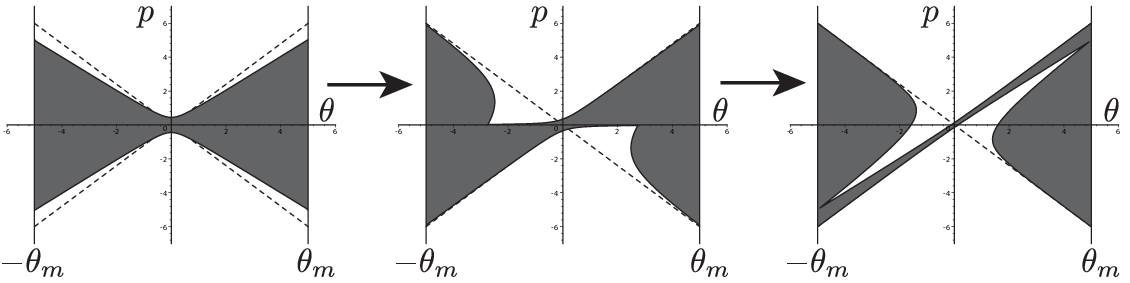
(I) , .
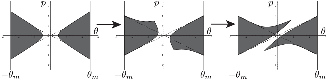
(II) , .
2.4.3 More on departure from adiabaticity
In this subsection, we come back to the issue of the role played by the quantum critical point in quantum quench dynamics (QQD). This has been discussed in several contexts: e.g. (a) how the asymptotic density of excitations scales as a function of the parametric distance from criticality when the initial hamiltonian is at criticality (see [11]), or (b) how the asymptotic QQD value of some observable or order parameter differs from the adiabatic value, as a function of (in our notation) (for given fixed ). In the above subsections, we found many examples of differences between QQD and adiabatic evolution. We explore this aspect more in this subsection by studying the behaviour of . We find that as is taken further away from towards the other side of the quantum critical point, the departure from adiabaticity becomes appreciable from near . We have found similar behaviour for the higher moments etc. as well. This phenomenon of departure from adiabaticity around the critical point is similar to that reported in [12] in the context of QQD in a Hubbard model. Indeed our Fig. 7 is quite similar to Fig. 3 of [12].1818 18 The departure from the adiabatic curve does not exactly coincide with criticality in [12] or in our work here, an effect which is more pronounced for higher moments. This points to some possible universal role played by the quantum critical point even in dynamical phenomena.
 (a)
(a)
 (b)
(b)
|
3 Double trace model
Like the single trace model, the double trace model (3), can also be described (see (35)) in terms of fermions moving in one spatial dimension. The hamiltonian is given by
| (15) |
The difference from the single trace case is that the fermions are now interacting with a mutual potential. Since this is an interacting system, it is not obviously integrable; we will not explore the question of integrability in this work.
Before going to explore dynamics in this system, we will briefly review its connection to 2D adjoint scalar QCD and string theory.
The 2D adjoint scalar QCD:
Consider the following two dimensional gauge theory on a [13],
| (16) |
Here is the period of the . This theory is related to a dimensional reduction of dimensional pure Yang-Mills theory (which, for , can be related to D2 branes compactified on a Scherk-Schwarz circle)1919 19 If we derive the model (16) from the higher dimensional gauge theory or D branes, additional terms are induced through quantum loop effects. For this reason, the coupling at the two dimensional gauge field and the commutator interaction have been distinguished in the model (16). The most relevant term in these loop corrections in weak coupling is the mass term for the adjoint scalar. We omit this mass in this paper as argued in [13].. The thermodynamical phase structure of this model is as shown in Fig. 8. At sufficiently large , (at least above the critical line so that the system is confined, ), the adjoint scalars would have a mass gap and are integrated out through the expansion [13] (see also [14, 15]). The theory is then described by the following effective action
| (17) |
where , and is the modified Bessel function of the second kind. In the following subsections, we would mainly consider dynamical phase transitions near the critical line in Fig. 8. In this case, we can ignore the higher modes () in the infinite sum in the potential term, and obtain the double-trace model (3) or (15). Thus the model (15) describes the dynamics of the spatial Polyakov loop of the QCD (16) in the confined phase. Here in (15) is a function of the parameters in the QCD, and importantly it monotonically decreases as increases [13].
Phases:
The parameter determines the phase structure of the theory (15). For high enough (), the attractive potential dominates and the system is gapped. For low enough (, the kinetic term dominates and the system is gapless. See Fig. 8 (b) for more details.
 (a) Phase structure of 2D adjoint scalar QCD (16).
 (b) A plot of free energy around line of diagram (a).
|
3.1 Dynamical evolution
In case of the double trace model, several solutions have been derived for a given () as shown in Fig. 8 (b) but the ground state is always unique. Hence we naively expect that the unstable or meta-stable solutions may evolve toward the ground state if we add sufficient perturbations to these solutions. We will explore the question of possible dynamical phase transition as well as the question of relaxation in this process. In this section, we use the semiclassical approximation and consider only the large- case. (See the details in Appendix E.)
3.1.1 Dynamical evolution from the uniform gapless phase
We will consider the time evolution of the uniform phase. In terms of the droplet picture (Section A), the uniform phase is given by
| (18) |
This configuration is always a solution of the model (15), since the force term vanishes for particles located uniformly on the circle. In order to have non-trivial dynamics, we add a small perturbation to this configuration.
Before we discuss the actual results of the evolution below, let us pause and ask what to expect. If in (15) was small enough, say well below , for such values of the uniform phase is the ground state. Thus, we expect that for small enough amplitude of the perturbation, the system will revert back to the uniform phase. Indeed for , discussed in Section 2.2, we find this to be explicitly true.
On the other hand, we are interested here in values of
above where the ground state is the gapped one.
Thus, we will expect the
perturbation to be unstable towards formation of a
gapped phase.
Order parameter: Since all moments (9) of the
density vanish in the uniform phase, any of these, say , can be
considered as an order parameter, which would change from if the distribution changes from uniform to a
non-uniform solution.
Note that we consider symmetric () perturbations only in this article.
Then we can take by a gauge choice.
We will now discuss the actual result of the time-evolution of a perturbation according to (76). In Fig. 9, the result is presented for , at which the uniform solution (18) is unstable. Then develops to a non-zero value (see the right panel of the figure), and we obtain a non-uniform distribution. However the distribution does not develop a gap, unlike the naive expectation above. Indeed, just as in Fig. 6, part (I), the gapless gapped transition is once again not possible since the droplet in phase space does not split. In addition to all this, we also find evidence for equilibration in (see the right panel) which indicates relaxation of the phase space configuration to one with a thin stable neck.2020 20 The ‘neck’ avoids a gap-opening transition, and consequently avoids a dynamical singularity. It is important to explore this further, particularly in the context of the double scaled matrix model. For similar issues related to smoothening of singularities through effects, please see [17, 18].


|
3.1.2 Time evolution from the gapped phase
The discussion is analogous to the previous case. We consider a meta-stable gapped state at (Phase III in Fig. 8 (b)) and perturb the system.
The result at is shown in Fig. 10. A dynamical gapped gapless transition takes place. Thus, like in the single trace case, we once again see a one-way dynamical phase transition, gapped to gapless, but not gapless to gapped. This once again, has a clear interpretation in terms of phase space.
Note that if the perturbation is not sufficient, the state reverts back to the original gapped configuration, since the configuration is meta-stable.


|
3.1.3 Appearance of exotic states
We have considered the time evolutions of unstable/meta-stable solutions by adding perturbations. However if we add sufficiently large perturbations, we observe appearance of exotic asymptotic states. See Fig. 11, e.g., where in the middle panel two blobs of fermions have appeared, which are moving towards the left and the right respectively. As time progresses, the two blobs keep executing a period motion and in coordinate space, this means that two density peaks approach, merge and separate out, and repeatedly pass through each other like colliding solitons (remember that in our model the fermions are moving in a circle).


|
Another exotic time evolution can be seen if we consider the higher modes of the potential (17). We assume appropriate values of and small such that is large, consequently the gapped solution is stable and the uniform one (18) is unstable. In this setup, the unstable uniform solution (18) evolves as shown in Fig. 12. In this case, the dynamical phase transition consists of two steps. First the unstable uniform state decays to a 2-peak state (where the ‘peaks’ refer to those in the coordinate space density . This 2-peak state remains for some time, and finally decays to the one-peak state. We have also observed appearance of various multi-peak intermediate states if we change the initial perturbations.
Indeed the existence of unstable multi-peak solutions for the small region in Fig. 8 (a) and the possibility of their appearance during the decays of the unstable uniform solution have been predicted in [19]. Our result confirms this conjecture. Interestingly similar time evolutions have been observed in the decay of black string in the Gregory-Laflamme transition also [20, 21]. An unstable black string does not always decay directly to a single-black hole, which is thermodynamically most stable, but to multiple black holes in some cases.


|
Note that the two-peak state that appears in Fig. 12 is qualitatively different from the breather-like asymptotic state in Fig. 11. The former state is approximately static (with two distinct, long-lived density peaks around ) until it decays to a single-peak state, whereas the latter state is approximately stationary and the two peaks merge and separate out repeatedly in an oscillatory fashion. (See the movies for these evolutions from the link in footnote 4.)
As we have seen in section 2, the system is integrable if the double trace interactions are turned off. One open question is whether this interaction breaks the integrability. The appearances of these exotic asymptotic/intermediate states may shed light on this issue. Especially the exotic asymptotic states in Fig. 11 may imply an attractor structure in this system. We will come back to this issue in a future work.
4 Discussions
The results of our paper have already been summarised in Section 1 and described in Sections 2 and 3. In this section, we will describe some related issues, speculations and outstanding questions.
4.1 Duality to 2D string theory and algebra
The model defined by Eqs. (25), for fixed , is essentially the matrix model. This model (in its double-scaled form: ), has a string theory ‘dual’, namely the two-dimensional bosonic string theory, which is characterized by a massless scalar field (called ‘tachyon’) on a flat spacetime and linear dilaton background (see, e.g. the review of [22]). The tachyon field fluctuation is given by a non-linear and non-local transformation of the matrix model scalar field fluctuation (see, e.g., [23, 24, 25] for more details). The filled Fermi sea, , , is a solution of (28), and corresponds to the tachyon vacuum in string theory. In quantum quench dynamics, in the matrix model description, we start with an unstable density perturbation, which evolves in time under the restoring force towards the above-mentioned stable configuration. Since the motion is conservative (in fact, it has an infinite number of conserved quantities), the configuration cannot reach the stable configuration; in stead there is an oscillatory motion, in which lower frequency modes transfer energy to the higher frequency ones, leading to an energy cascade as discussed in Section 2.2.2121 21 We show this in the unitary matrix model, but we find similar behaviour also in the Hermitian matrix model which is directly identified as the matrix model.
It would be interesting to map this oscillation to string theory tachyon modes by applying the transformation alluded to above. We expect that qualitatively it would be a similar phenomenon to the one found in the matrix model, with a finite energy extended configuration giving rise to proliferation of high frequency modes, asymptotically approximated by a general Gibbs ensemble (GGE) in spacetime. Note that in the 2D string theory too, there are an infinite number of conserved charges, which are the diagonal elements of an infinite dimensional algebra, viz. the algebra (see [26]), thus making the GGE a natural choice of ensemble. It is an interesting question whether the GGE can be represented by a new field configuration such as a non-trivial solitonic configuration, or a black hole.2222 22 It has been argued that inflaton oscillations around its vacuum configuration, which is analogous to the tachyon oscillations described above, can produce primordial black holes (see [27], for example). We discuss the black hole scenario in some detail in the subsection 4.3 below.
In [28], a different, type 0, 2D string theory is proposed as dual to the (gauged) hermitian model (25), where the singlet condition is ensured by a gauge covariant kinetic term . In the context of the type 0B theory, there are two massless scalars, the tachyon and an axion. We expect many of the comments in the previous paragraph to go through in this case as well.
4.2 Gravity duals of other integrable systems
The phenomena of selective equilibration and emergence of GGE studied in this paper would be of interest in many other examples of integrable systems with gravity duals. We mention below a few of them.
D1-D5 system:
The D1-D5 system (reviewed in, e.g. [29]) is described, at a certain point of its moduli space, by a free 2D CFT (with target space an orbifold of the type , where or , and ). The usual D1-D5 supergravity solution is located at a different point of the moduli space, which can be reached by introducing a marginal interaction to the free CFT at . There are certain nonrenormalization theorems which ensure the protection, under the -deformation, of a number of quantities including black hole entropy and absorption cross-section. In [30] a certain response function in the integrable theory is exactly computed and shown to agree with its gravity dual, namely the absorption cross-section of the two-charge black hole (at the supergravity point). The agreement is found only in the large limit and using a coarse-grained probe. The field theory calculation seems to be well-suited for a GGE description.
Giant gravitons:
The half-BPS configurations of SYM on are described by a complex matrix QM in a harmonic oscillator potential which can be described by free fermions [31, 32] in a manner similar to that described in this paper. The gravity duals are the well-known LLM geometries [33], which can be described in terms of giant gravitons [34, 35, 36] in the probe approximation.
Higher spin duals of 2D CFT’s:
Recently, [37] has proposed a duality between the large limit of certain 2D CFT’s called the minimal models (represented by the coset WZW models ) and a one-parameter higher spin (Vasiliev) theory parametrized by (see, e.g. the review [38]). The limit corresponds to 2D relativistic free (complex) fermions and is very similar to the system described in this paper.
D2 branes:
The gauge theory system (16) was considered in [13], where a gravity dual is discussed (see Section 5 of that paper) in terms of the near horizon geometry of D2 branes compactified on a ‘Scherk-Schwarz circle’ (i.e. a small spatial circle of size with antiperiodic fermions). The other two directions are periodic, with sizes , which characterize the phase diagram of the model is given in Fig. 8 (a). As discussed in [13], the low temperature phase of the model is described by a soliton solution wrapping the temporal circle uniformly, while the high temperature (‘deconfinement’) phase, , is given by a localized soliton. We clearly find evidence of equilibration in the low temperature phase of the field theory in Fig. 9 (a). It is also known that the deconfinement phase shows dissipation. It would be interesting to understand such equilibration in terms of the solitonic geometries which obviously do not have a horizon.
super Yang Mills theory:
This is clearly one of the most important examples of integrable models in AdS/CFT [39]. The giant gravitons described above describe a special sector of this model. More generally, operators of super Yang Mills theory whose energies do not scale with , can be mapped to states in integrable spin chains which possess an infinite number of conserved charges. For energies the integrability does not persist; thus, a generic perturbation equilibrates, and is described in the gravity dual by black hole formation (see, e.g., [40]). The present discussion opens the possibility of equilibration of certain perturbations in the integrable subsector and emergence of a GGE; it would clearly be of interest to find a gravitational dual of such an ensemble, if any.
4.3 Black holes and entropy
It is tempting to speculate that the equilibration, discussed above for the matrix QM model, and possibly generalizable to other integrable field theories, is described in terms of formation of black holes in a dual theory. In many known examples of AdS/CFT, equilibration does have a natural interpretation in terms of formation of black holes2323 23 or, in the context of a probe approximation, in terms of the damping of quasinormal fluctuations in a black hole background..
Such a scenario, however, must pass the following stringent
tests:
(i) Black holes are typically not associated with integrable
models; while the latter have an infinite number of conserved charges,
black holes typically have only a few (cf. uniqueness
theorems). Since a GGE (38) is characterized by an infinite number
of chemical potentials, any black hole describing a GGE must also have
an infinite number of parameters.
(ii) The entropy of the GGE must
match the entropy of the known black holes.
(iii) Besides the static
black hole solution, there must be a dynamical collapse solution which
would capture the equilibration process. The black hole formation time
should then match the time of relaxation to equilibrium described by
the GGE.
(iv) A non-extremal black hole will Hawking radiate; there
must be an interpretation of the two-stage process— formation and
evaporation— in the field theory description.
(v) In case we seek
a description of equilibration and dissipation in terms of absorption
of energy by a fixed black hole background in the dual geometry.
2D:
As mentioned above, the matrix model
(25), is dual to the 2D bosonic string theory, in the linear
dilaton background. This theory, as described by its massless fields
(the metric, dilaton and the massless ‘tachyon’), does have the MSWW
black hole solution [41, 42] (see
[43, 44] for superstring
generalizations). Let us discuss the above points to see whether this
black hole can be relevant for a description of the GGE found in the
present paper.
Point (i): the MSWW black hole solution, is indeed
the unique solution of the effective field theory of massless modes of
2D string theory, and is specified by only the mass
parameter 2424
24
The charged cousins described in
[43, 45] require fluxes which can come from
superstring or type 0 theories. However, this solution can be
extended to an infinite-parameter generalization in 2D string field
theory [46]. Each such black hole possesses an
infinite number of specified charges (corresponding to
charges of higher mass non-propagating gauge fields), and could
potentially correspond to a given GGE with fixed values of the
chemical potentials.
Point (ii): the entropy of the MSWW black hole
was found to be (see [45]) of the order of , whereas the entropy of the GGE in Section 2.3
turns out to be of order .
Point (iii):
[47] has argued that if we wish to form the MSWW
black hole (or its type 0B counterpart) by collapsing a tachyon shell,
physics becomes strongly coupled even before a horizon is formed. In
the type 0B black hole, one can in stead consider collapse of an axion
shell; in this case, there is no strong coupling problem but the shell
is scattered back to infinity from near the incipient horizon and a
black hole is not formed.
Point (iv): Reference
[47] performs a matrix model
computation to rule out any Hawking radiation from a possible gravitational
collapse of axionic matter.
Point (v): a fixed black hole
background in type 0A theory was argued in [43] to be
dual to a deformed matrix model [48]. One could in
principle consider fermionizing such a model (as in (20)), explore
dissipation in this, and attempt to explain this in terms of black
hole absorption. However, doubts have been raised in
[49] about the duality, as the entropy of the matrix
model is computed there to be whereas the entropy of the black
hole is . The suggested dual matrix model, according to
[49], which reproduces an entropy, is the one
proposed in [50]; however, in this model, the
off-diagonal matrix elements play a crucial role, and the model is not
(at least in any obvious sense) integrable any more. One
could also consider the proposal in [24] for construction of
a black hole background in terms of an asymmetrically filled Fermi sea.
We leave further studies of these issues for the future.
Higher spin black holes in AdS3:
We have already discussed above the duality between large 2D CFT’s ( minimal models) and higher spin (Vasiliev) theories in AdS3. In the limit of , the field theory is that of number of complex free fermions, and is likely to equilibrate as in this paper, with emergence of GGE. As in case of the 2D gravity duals, the AdS3 also has black holes, the most well-known being the BTZ black hole. Indeed, it has been found in [51] that the BTZ black hole has spin three and spin four generalizations. It would be very interesting to investigate if this result generalizes to arbitrarily high spin, in which case they would be natural candidates for a dual description of GGE. These black holes have an entropy of , matching the central charge of the field theory (see [52], e.g.), which agree with the entropy of the GGE computed in this paper.
The superstar geometry:
In the context of the matrix model-LLM-giant graviton duality mentioned earlier, thinned out phase space configurations such as (73) in which the fermion occupation numbers are fractional have been studied. The resulting LLM geometries are singular and are called superstar geometries. These geometries have zero horizon area, but a Bekenstein entropy can be assigned to a stretched horizon [53], which turns out to be just like the standard Boltzman formula for entropy in these systems, and agrees with the GGE estimate of entropy.
D1-D5:
The possible relevance of GGE to the two-charge D1-D5 black hole is already mentioned in the previous subsection. The entropy of the two-charge black hole appears to agree with the entropy of GGE.
4.4 Topology change and the Gregory-Laflamme phase transition
The uniform and gapped phases of the double trace model (3) correspond to the large and small sides of the phase boundary AB in Fig. 8 (a). These phases, by definition, refer to the uniform and clumped eigenvalue distributions of the spatial Wilson line , which arises from the gauge of theory of D2 branes wrapped on a small Scherk-Schwarz circle. (see page 4.2). What do these phases mean in gravity? This question was investigated in detail in [19, 54, 55, 56] (see [14, 57] for other related references). The Euclidean near-horizon description of such a system at large and (sizes of the temporal and spatial circles, respectively) is that of a D2 soliton. If we T-dualize this system along the large spatial circle, we get a D1-brane soliton which is uniformly smeared along a small dual circle . This is the description of the phase to the right of the line AB in Fig. 8 (a); now as we decrease , the dual circle starts to increase and the uniformly smeared D1 soliton starts getting stretched and as increases beyond a certain critical size, it becomes unstable towards breaking and forming a localized soliton. In [58], Gregory and Laflamme predicted such a transition as a thermodynamic phase transition[59, 60, 61, 62]. Thus, the dynamical gapless gapped transition in our model translates to a dynamical GL transition from a uniform to a localized soliton. In particular, the observed non-existence of such a transition in the matrix model, ultimately due to non-splitting of Fermi liquid droplets, implies impossibility of a dynamical GL transition from a 1-brane (uniform soliton) to a 0-brane (split solution).
The original context of the GL transition was in the context of a clumping transition of a black string into a black hole. The question about whether this can happen dynamically is related to the issue of cosmic censorship and the appearance of a naked singularity, and has been discussed extensively in the literature [20, 21, 63, 64, 65, 66]. In a supersymmetric variant of (16), the phase transition discussed in the previous paragraph would correspond to such a transition from a black string to a black hole. Since the technique developed in this paper appears to be fairly robust, dynamical transition in this model could share similar features, and could shed light on the issue of dynamical appearance of a naked singularity. See also the related discussion in page 2.4.2.
4.5 Non-ergodic time evolution in confinement geometries
Very recently, non-linear instabilities of global AdS geometries under perturbations are actively studied [67, 68, 69, 70]. There, depending on initial perturbations, the perturbed geometries evolve to small black holes, boson stars, or geons [71]. Since the final states depend on initial conditions, the time evolutions are non-ergodic. Since global AdS would correspond to a confinement phase in the dual gauge theory, the appearance of these non-ergodic evolutions sounds reasonable. Especially, they would be related to the non-ergodic time evolutions in the D2 brane model (16) in the confinement phase, as argued in section 3. Since the gravity dual of the ground state (which is in confinement phase), is a soliton geometry, as shown in [13] based on the Witten’s holographic QCD, we presume that the non-ergodic time evolutions would be observed in this soliton geometry too. Then we can directly compare the time evolutions in the confinement phase in the gauge theory and the time evolutions in the soliton geometry. This would be an interesting new direction of the gauge/gravity correspondence, since we can calculate both explicitly.
Acknowledgement
We would like to thank Sumit Das, Kedar Damle, Avinash Dhar, Rajesh Gopakumar, Sourendu Gupta, Hideo Kodama, Hong Liu, Subhabrata Majumdar, Shiraz Minwalla, Krishnendu Sengupta, Spenta Wadia and Xi Yin for discussions. We also thank Pallab Basu, Manavendra Mahato and Spenta Wadia for collaboration on some earlier calculations which have overlaps with Section 3 of the present work. We would like to thank Sumit Das, Avinash Dhar, Rajesh Gopakumar, Shiraz Minwalla and Spenta Wadia for a careful reading of the manuscript and for important feedbacks. We would also like to thank user support team of Strategic Programs for Innovative Research (SPIRE) Field 5 “The origin of matter and the universe”, especially Satoru Ueda for helping our numerical calculation in Section 2. We also thank Lowell D. Johnson, who is the contributor of the GSL Mathieu function routines, for useful advice about the routines. The work of T.M. is supported in part by Grant-in-Aid for Scientific Research (No. 24840046) from JSPS.
Appendix A Fermionic formulation of MQM
In this appendix, we will discuss the fermionic formulation of MQM. For a general review, see, e.g. [22, 72].2525 25 For specific details of the material presented here, see, e.g. [73, 74, 75, 76, 77, 78, 79].
A.1 Single trace model
Let us first consider the single-trace model (2). The singlet sector of this model (see footnote 2) is described by the following -fermion action and hamiltonian
| (19) |
The positions are defined on a circle, and arise from the eigenvalues of diag; the fermionic nature arises from the measure (after integrating out the ’s) which vanishes for coincident eigenvalues. The identification of as comes from the partition function in (1).
A second-quantized version of the above action is written down:
| (20) |
It is useful to describe states of the system in terms of expectation value of the phase space (Wigner) distribution
| (21) |
We define the position space density as
| (22) |
The normalization condition in (20) implies that
| (23) |
Large- limit
Since , the large limit reduces to
| (24) |
In this limit, the fermion configurations are represented by a semiclassical Fermi liquid with a smooth phase space density and position space density; the expectation value is either 0 or 1 depending on whether the phase space cell (of vanishing area ) is occupied by a fermion or not). The regions with are called droplets of fermi liquid.
Phases:
Classically, due to the potential in (19) the particles tend to clump around ; quantum mechanically however the states of the system are quantized and Pauli exclusion tends to spread the fermions up. The competing tendencies dictate the qualitative nature of the ground state: (a) For , the potential is strong and the eigenvalues are clumped around . Pauli exclusion forces the fermions to occupy levels, but the Fermi level is below the top of the potential. This leads to a gap in around . This is called the gapped phase. (b) For the potential is weak and the eigenvalues are spread out (non-uniformly). The Fermi level is above the top of the potential and there are no gaps in . This phase is called a gapless phase. The phase transition at is characterized by the closing of a gap, when the Fermi level comes up and touches the top of the potential. This is a third order phase transition and was found in [2].
Double scaling:
It is clear from the above that the position of the fermi level , measured from the top of the potential, is . It turns out that the singularity of the free energy is the form . The double scaling limit is defined by , such that is held fixed. Our result about the entropy is without taking into account such a double scaling.
The hermitian model:
The double scaling limit captures the universal part of the potential near the top: , whose essential features can be equally simply reproduced, by replacing by () in (19); dropping the 1, the potential becomes , which is equivalent to the (singlet sector of the) hermitian matrix model
| (25) |
This model is called the matrix model.2626 26 The periodic boundaries need to be supplanted by to make the model well-defined; the choice of is not particularly relevant and does not affect critical/universal quantities. The double-scaled model is mapped to two-dimensional bosonic string theory (see the review [22]) by identifying . A similar duality to two-dimensional type 0 theories also exists (see the review [72]).
Classical droplet motion:
Suppose that the Fermi liquid configuration is that of a single droplet (e.g. the Fermi sea or a continuous distortion of it), characterized by specifying two functions , which demarcate the upper/lower boundaries of the droplet at a specific value of at time , i.e
| (26) |
Using this, we get the following formulae for density, momentum density and energy density:
| (27) |
Here for the unitary matrix model (2), (20), whereas for the hermitian matrix model (25). It turns out that are canonically conjugate variables, with Poisson bracket
This can be derived from the anticommutation relation of the fermion field, or from the symplectic structure of the -fields (see [78, 79]). The equation of motion of the ‘collective fields’ or follow from the above hamiltonian and Poisson brackets (see comments below (32) for limitations of the collective field description):
| (28) |
These equations of motion (EOM) can alternatively be derived from that of the phase space density
| (29) |
which, viewed from the particle-fixed frame, is simply the particle EOM, and can be regarded as the Euler equation or the dissipationless Boltzman equation. This viewpoint provides an explicit solution of the equation of motion:
| (30) |
where is the unique initial phase space point at which reaches at time through the dynamical evolution (19), and is the phase space density at . For the hermitian model (25), , and (30) becomes
| (31) |
which can be easily verified to be a solution of (29) for . In the special case of (free fermions with zero potential), we get
| (32) |
Note that the collective field equations of motion (28) depend on the assumption of a quadratic profile (26), which are clearly violated by ‘folds’ e.g. in Fig. 6 and Fig. 13. As a result, they are not valid for long times (see [78, 79]). In our actual analysis where we are specially interested in long time evolutions, we do not use (28) but use (29) or equivalently the particle equations of motion in Appendix E.
A.2 Double trace model
Using the fermionization techniques discussed in the previous subsection, the action (3) can be written as (with , as before)
| (34) | ||||
| (35) |
The definition of , all remain as before.
| (36) |
Because of the limitation of the collective field description in the presence of folds (see comments below (32)) for computation of the time evolution we use the equation of motion of the phase space density or equivalently the particle equations of motion as in Appendix E.
Appendix B Integrability and GGE
The single-trace model (19), (20) is clearly integrable, since it consists of free particles. Classically one can consider the energy of each particle, , to be an ‘action’ variable. Quantum mechanically, each linearly independent -fermion state can be specified by saying which single-particle energy levels, , are occupied. The quantities
| (37) |
are all constant in time, and commute with each other. For finite , only of them, is enough to determine the energy levels (up to some discrete ambiguities which we shall ignore), hence are all dependent on the first ’s. In the limit, of course, the charges (37) are all independent.
We can define the Generalized Gibbs Ensemble (GGE) in terms of the conserved charges as follows:
| (38) |
Here are chemical potentials. For more details, see [1].
In the present discussion, it is convenient to introduce the fermion occupation numbers , , where if the single particle energy level is occupied, and if it is not (note that our fermions are spinless, and that the energy levels are non-degenerate). These can be defined in terms of the creation/annihilation operators through the equations
| (39) | ||||
| (40) |
In terms of the ’s, . For , in stead of (37), one can use ’s as the (independent) conserved charges, which leads to the following definition of the GGE:
| (41) |
With this definition, we get, by explicit evaluation (see [80]),
| (42) |
which gives a remarkably simple Fermi-Dirac distribution which involves only one chemical potential. The chemical potentials are now trivially found:
| (43) |
The entropy of the GGE is given by
| (44) |
The GGE hypothesis is that, if we start from an appropriate excited state , there exists a certain class of observables such that, as
| (45) |
where the GGE is defined by the charges
| (46) |
or equivalently by the chemical potentials , determined through (43).
Note that if the initial state is an eigenstate of the number operators , then by (46), or . The GGE constructed from such an initial state has vanishing entropy , according to (44).
B.1 Verification of the GGE hypothesis for
We wish to verify (45) where the observable is the density variable
where , . The LHS of (45) becomes, in the Heisenberg picture,
| (47) |
where represents expectation value in the initial state . We will evaluate this expression in (57) where the initial state is prepared according to QQD. The large limit of (47) is given by the semiclassical expression (33).
To compute the RHS of (45) for , first note that
| (48) |
where . Using this and (39), we get
| (49) |
Note that this is independent of time, as expected. Here are to be determined from their values in the initial state
| (50) |
Thus,
| (51) |
Since these uniquely determine the chemical potentials through (43), the GGE is specified completely.
B.2 Phase space density in GGE
Appendix C Quantum quench dynamics (QQD)
Suppose we consider a sudden change of the parameter in the single-particle hamiltonian (19), from at to at . Time evolution works as follows. We consider the ground state of the system (Fermi sea in this case) appropriate to the parameter for . Quantum quench dynamics refers to the sudden approximation in which the system evolves for according to the new parameter , from an initial state equal to the old Fermi sea
| (53) |
Clearly the system is integrable after and our discussion in the previous section applies (we need to identify the parameter with ).
We wish to compute the time-dependence of
| (54) |
for . Here the second expression is in the Heisenberg picture (in which the state remains the initial state (53)), while the third expression is in the Schrodinger picture in which is the time evolution of (53) according to the new Hamiltonian.
To proceed, let us express the old Fermi sea in terms of eigenstates in terms of the new number operators . Suppose we denote the eigensystem of the old hamiltonian (with ) as . The functions can clearly be written in the new eiganbasis : thus
Just like (39), the Fermi field can be equally well expanded in terms of ; thus
| (55) |
we get
| (56) |
Using the expression (47) we get
| (57) |
where we have used (56) and the defining property of the old Fermi-sea:
| (58) |
We explore (57) numerically in the text for various values of . The limit can be computed in the semiclassically in the droplet picture as in (33).
C.1 GGE for QQD
We wish to compute in the context of QQD, using the general expression (51), for the initial state (53).
C.2 Adiabatic time evolution
Suppose we have a time-dependent Hamiltonian , e.g. (20) with -parameter, or (35) with -parameter. Suppose the time-dependence starts after some time ; we wish to study the time-evolution of a wavefunction , which at is an eigenstate: = . QQD is an example in which the time-variation is in the form a step function at . An adiabatic time evolution, on the other hand, refers to a sufficiently slow time-variation such that one can approximate as the instantaneous eigenstate of with eigenvalue ; this notion is well-defined in the absence of level crossing, which can be ensured if the spectrum is discrete which sets a finite time scale. In the examples considered in this paper, we are often interested in the time-evolution of the ground state, and by an adiabatic expectation value we will always mean expectation value in the instantaneous ground state = .2727 27 At a critical point, the spectrum is gapless; there we will simply define .
In the context of (20), the ground state of a specific value is clearly given by, in an obvious notation where we denote all instantaneous quantities by an additional subscript
| (61) |
By expanding in this new basis, we get
| (62) |
The time dependence of the adiabatic quantity is reflected in the appearance of the instantaneous eigenfunctions.
Appendix D An analytic calculation of relaxation
In this section, we will consider time evolution in the single-trace model (2) with . (This model is also equivalent to in (3).) In this case, the ground state is given by (see (27) for notation).2828 28 Note that this corresponds to , which obviously satisfies (28) for . Suppose we perturb the ground state configuration at by a sinusoidal deformation
| (63) |
where is the amplitude of the perturbation (see Fig. 13). We wish to evaluate the time evolution of this perturbation using the action (20) with .

We will evolve the configuration as in (32), which essentially says that ; in other words, to get any point of the evolved Fermi surface at time , we should simply evolve points on the initial Fermi surface according to the equation of motion of (19) with , which is given by
| (64) |
In order to solve this equation for points on the Fermi surface, it is convenient to employ a parameter and rewrite the initial configuration (63) as 2929 29 From now, we omit , since we can derive it trivially from .
| (65) |
Then from (64) we obtain the Fermi surface at time as
| (66) |
This solution with is plotted in the middle of Fig. 13; the ‘folds’ appear because of the stretching caused by different speeds of fermions at different heights from the -axis. As time progresses, more or more ‘folds’ keep appearing.
In the perturbation (63), only is excited and other are zero. We evaluate how these modes behave as increases. From the solution (66), we calculate the -th moment as3030 30 The expression in the first line in this equation is crude, since the droplet has many folds at a late time as shown in the center of Fig. 13 and we need to subtract the white region below . However after the change of the variable from to , this subtraction is automatically involved.
| (67) |
These integrals will be given by the Bessel function . For example, if , the integral (67) with and are evaluated as
| (68) |
For large , they decay with as
| (69) |
and
| (70) |
Other also exhibits a similar decay. In Section 2.2 we will compare the time-evolution of various modes and find a picture of an energy cascade in which lower frequency modes die out before the higher frequency modes, causing a transfer of energy from higher to lower frequencies, in a manner similar to energy cascades in turbulence.
D.1 Asymptotic and GGE form of the Fermi surface
As we mentioned below (66), the asymptotic form of the droplet consists of an infinite number of ‘folds’ which eventually densely fill an entire band. When suitably coarse-grained (the ‘grain’ size can be finer and finer as time progresses), this describes a thinned out Fermi liquid, as schematically plotted on the right of Fig. 13.
Since we have already verified the GGE hypothesis of our system for the density variable, let us describe the above ‘thinned out’ Fermi liquid in terms of the GGE. We begin with the GGE value (52) of the phase space density. The single-particle Hilbert space can be labelled by the momentum wavefunctions
which trivially gives , and hence by (52) (keeping the notation implicit)
| (71) |
We can identify as the momentum-space density
| (72) |
We can compute ’s from a given initial quantum state by using (50). However, the calculation is much better done semiclassically, when the initial state is given in terms of a classical droplet configuration (63). Note, first of all, that the momentum-space density (72) in the present case is a constant of motion. This is easy to see since and all fermions have a constant momentum so the momentum density remains constant.3131 31 It can also be seen from (29) and (72). We can, therefore, compute the momentum density from the initial configuration (63). Note that from (63) and (26) we can find out the initial value of and hence by using (72). The result of this calculation is 3232 32 Geometrically the RHS of (72) is given by where are the counterparts of in (26).
| (73) |
which gives us a quantitative representation of a ‘thinned out’ Fermi liquid on the right panel of Fig. 13.
D.2 Calculation of Entropy
We will now calculate the entropy . As we show in Appendix D.1, in the large droplet description, the ’s are given by (71). Combining with (73), and (44), we get
| (74) |
In the first equality, we have inserted a factor of 2 since the negative -axis contributes the same amount. Also we have used from (71). In the last step, note that only contributes to the integral, for which we use the value of in the third line of (73). Note that is exactly linear in (as well as in the amplitude of the initial perturbation (11)).
Appendix E Details of our numerical analysis
Exact computation
We use an exact computation for the single trace matrix model (2) at finite . In this case, the eigen function is given by the Mathieu function. We numerically evaluate this function by using GCC with the GNU Scientific Library.
Semiclassical computation
For the single trace matrix model (2) at large- and the double trace matrix model (3), we use a semiclassical approximation. At the strict large-, the dynamics of the matrix models are described by the droplet in the phase space. We discretize the support of the initial droplet by uniformly distributed points (we take to be .) Each of these points is then evolved according to the classical equation of motion
| (75) |
for the single trace model (2), and according to the classical equation of motion
| (76) |
for the double trace model (3). Here and () are the points of the discretized droplet. Evolving these points in this fashion is equivalent to a discretization of the Euler equation (29). By using the Runge-Kutta method, we solve these equations with a given initial condition3333 33 In the case of the single trace model, the motion of the surface of the droplet is sufficient to determine the dynamics of the model, since the particles are free. In addition, analytic solutions of the equation of motion (75) are given by elliptic functions, and can be used to significantly improve the calculation of droplet motion. Indeed we use this idea to plot Fig. 6 in the hermitian matrix model (25). . Note that the above use of the classical equations means that we are in the strict large- limit. As a result, the number , which is simply a measure of discretization of the classical phase space, is not related to in the original matrix model (while measures quantum effects, measures some discretization error of classical equations).
References
- [1] A. Polkovnikov, K. Sengupta, A. Silva and M. Vengalattore, “Nonequilibrium dynamics of closed interacting quantum systems,” Rev. Mod. Phys. 83, 863 (2011) [arXiv:1007.5331 [cond-mat.stat-mech]].
- [2] S. R. Wadia, “N = Infinity Phase Transition In A Class Of Exactly Soluble Model Lattice Gauge Theories,” Phys. Lett. B 93, 403 (1980).
- [3] D. J. Gross and I. R. Klebanov, “One-dimensional String Theory On A Circle,” Nucl. Phys. B 344, 475 (1990).
- [4] S. R. Das, “Holographic Quantum Quench,” J. Phys. Conf. Ser. 343, 012027 (2012) [arXiv:1111.7275 [hep-th]].
- [5] C. Asplund, D. Berenstein and D. Trancanelli, Phys. Rev. Lett. 107 (2011) 171602 [arXiv:1104.5469 [hep-th]].
- [6] P. Riggins and V. Sahakian, “On black hole thermalization, D0 brane dynamics, and emergent spacetime,” Phys. Rev. D 86, 046005 (2012) [arXiv:1205.3847 [hep-th]].
- [7] C. T. Asplund, D. Berenstein and E. Dzienkowski, “Large N classical dynamics of holographic matrix models,” arXiv:1211.3425 [hep-th].
- [8] D. J. Gross and E. Witten, “Possible Third Order Phase Transition In The Large N Lattice Gauge Theory,” Phys. Rev. D 21, 446 (1980).
- [9] S. R. Wadia, “A Study of U(N) Lattice Gauge Theory in 2-dimensions,” arXiv:1212.2906 [hep-th].
- [10] Pasquale Calabrese, Fabian H. L. Essler, Maurizio Fagotti, “Quantum Quench in the Transverse Field Ising Chain,” Phys. Rev. Lett. 106, 227203 (2011) [arXiv:1104.0154[cond-mat.str-el]]
- [11] R. A. Barankov, “Quench dynamics as a probe of quantum criticality,” arXiv:0910.0255 [cond-mat.stat-mech]
- [12] K. Sengupta, Stephen Powell and Subir Sachdev, “Quench dynamics across quantum critical points” Physical Review A 69, 053616 (2004) [cond-mat/0311355].
- [13] G. Mandal and T. Morita, “Phases of a two dimensional large N gauge theory on a torus,” arXiv:1103.1558 [hep-th].
- [14] O. Aharony, J. Marsano, S. Minwalla, K. Papadodimas, M. Van Raamsdonk and T. Wiseman, “The phase structure of low dimensional large N gauge theories on tori,” JHEP 0601, 140 (2006) [arXiv:hep-th/0508077].
- [15] G. W. Semenoff, O. Tirkkonen and K. Zarembo, “Exact solution of the one-dimensional non-Abelian Coulomb gas at large N,” Phys. Rev. Lett. 77 (1996) 2174 [arXiv:hep-th/9605172].
- [16] P. Basu, B. Ezhuthachan and S. R. Wadia, “Plasma balls / kinks as solitons of large N confining gauge theories,” JHEP 0701, 003 (2007) [arXiv:hep-th/0610257].
- [17] L. Alvarez-Gaume, P. Basu, M. Marino and S. R. Wadia, “Blackhole / string transition for the small Schwarzschild blackhole of AdS(5) x S5 and critical unitary matrix models,” Eur. Phys. J. C 48, 647 (2006) [arXiv:hep-th/0605041].
- [18] L. Alvarez-Gaume, C. Gomez, H. Liu and S. Wadia, “Finite temperature effective action, AdS(5) black holes, and 1/N expansion,” Phys. Rev. D 71, 124023 (2005) [hep-th/0502227].
- [19] T. Azuma, T. Morita and S. Takeuchi, “New States of Gauge Theories on a Circle,” arXiv:1207.3323 [hep-th].
- [20] M. W. Choptuik, L. Lehner, I. Olabarrieta, R. Petryk, F. Pretorius and H. Villegas, “Towards the final fate of an unstable black string,” Phys. Rev. D 68 (2003) 044001 [arXiv:gr-qc/0304085].
- [21] L. Lehner and F. Pretorius, “Black Strings, Low Viscosity Fluids, and Violation of Cosmic Censorship,” Phys. Rev. Lett. 105 (2010) 101102 [arXiv:1006.5960 [hep-th]].
- [22] P. H. Ginsparg and G. W. Moore, “Lectures on 2-D gravity and 2-D string theory,” In *Boulder 1992, Proceedings, Recent directions in particle theory* 277-469. and Yale Univ. New Haven - YCTP-P23-92 (92,rec.Apr.93) 197 p. and Los Alamos Nat. Lab. - LA-UR-92-3479 (92,rec.Apr.93) 197 p [hep-th/9304011].
- [23] M. Natsuume and J. Polchinski, “Gravitational scattering in the c = 1 matrix model,” Nucl. Phys. B 424, 137 (1994) [hep-th/9402156].
- [24] A. Dhar, G. Mandal and S. R. Wadia, “Discrete state moduli of string theory from the C=1 matrix model,” Nucl. Phys. B 454, 541 (1995) [hep-th/9507041].
- [25] A. Dhar, G. Mandal and S. R. Wadia, “String beta function equations from c = 1 matrix model,” Nucl. Phys. B 451, 507 (1995) [hep-th/9503172].
- [26] S. R. Das, A. Dhar, G. Mandal and S. R. Wadia, “Gauge theory formulation of the C = 1 matrix model: Symmetries and discrete states,” Int. J. Mod. Phys. A 7, 5165 (1992) [hep-th/9110021].
- [27] B. J. Carr, “Primordial black holes: Do they exist and are they useful?,” astro-ph/0511743.
- [28] M. R. Douglas, I. R. Klebanov, D. Kutasov, J. M. Maldacena, E. J. Martinec and N. Seiberg, “A New hat for the c=1 matrix model,” In *Shifman, M. (ed.) et al.: From fields to strings, vol. 3* 1758-1827 [hep-th/0307195].
- [29] J. R. David, G. Mandal and S. R. Wadia, “Microscopic formulation of black holes in string theory,” Phys. Rept. 369, 549 (2002) [hep-th/0203048].
- [30] S. R. Das and G. Mandal, “Microstate Dependence of Scattering from the D1-D5 System,” JHEP 0904, 036 (2009) [arXiv:0812.1358 [hep-th]].
- [31] G. Mandal, “Fermions from half-BPS supergravity,” JHEP 0508, 052 (2005) [hep-th/0502104].
- [32] Y. Takayama and A. Tsuchiya, “Complex matrix model and fermion phase space for bubbling AdS geometries,” JHEP 0510, 004 (2005) [hep-th/0507070].
- [33] H. Lin, O. Lunin and J. M. Maldacena, “Bubbling AdS space and 1/2 BPS geometries,” JHEP 0410, 025 (2004) [hep-th/0409174].
- [34] J. McGreevy, L. Susskind and N. Toumbas, “Invasion of the giant gravitons from Anti-de Sitter space,” JHEP 0006, 008 (2000) [hep-th/0003075].
- [35] M. T. Grisaru, R. C. Myers and O. Tafjord, “SUSY and goliath,” JHEP 0008, 040 (2000) [hep-th/0008015].
- [36] A. Hashimoto, S. Hirano and N. Itzhaki, “Large branes in AdS and their field theory dual,” JHEP 0008, 051 (2000) [hep-th/0008016].
- [37] M. R. Gaberdiel and R. Gopakumar, “An AdS3 Dual for Minimal Model CFTs,” Phys. Rev. D 83, 066007 (2011) [arXiv:1011.2986 [hep-th]].
- [38] M. R. Gaberdiel and R. Gopakumar, “Minimal Model Holography,” arXiv:1207.6697 [hep-th].
- [39] N. Beisert, C. Ahn, L. F. Alday, Z. Bajnok, J. M. Drummond, L. Freyhult, N. Gromov and R. A. Janik et al., “Review of AdS/CFT Integrability: An Overview,” Lett. Math. Phys. 99, 3 (2012) [arXiv:1012.3982 [hep-th]].
- [40] S. Bhattacharyya and S. Minwalla, “Weak Field Black Hole Formation in Asymptotically AdS Spacetimes,” JHEP 0909, 034 (2009) [arXiv:0904.0464 [hep-th]].
- [41] G. Mandal, A. M. Sengupta and S. R. Wadia, “Classical solutions of two-dimensional string theory,” Mod. Phys. Lett. A 6, 1685 (1991).
- [42] E. Witten, “On string theory and black holes,” Phys. Rev. D 44, 314 (1991).
- [43] S. Gukov, T. Takayanagi and N. Toumbas, “Flux backgrounds in 2-D string theory,” JHEP 0403, 017 (2004) [hep-th/0312208].
- [44] N. Berkovits, S. Gukov and B. C. Vallilo, “Superstrings in 2-D backgrounds with RR flux and new extremal black holes,” Nucl. Phys. B 614, 195 (2001) [hep-th/0107140].
- [45] C. R. Nappi and A. Pasquinucci, “Thermodynamics of two-dimensional black holes,” Mod. Phys. Lett. A 7, 3337 (1992) [gr-qc/9208002].
- [46] S. Mukherji, S. Mukhi and A. Sen, “Black hole solution and its infinite parameter generalizations in c = 1 string field theory,” Phys. Lett. B 275, 39 (1992).
- [47] J. L. Karczmarek, J. M. Maldacena and A. Strominger, “Black hole non-formation in the matrix model,” JHEP 0601, 039 (2006) [hep-th/0411174].
- [48] A. Jevicki and T. Yoneya, “A Deformed matrix model and the black hole background in two-dimensional string theory,” Nucl. Phys. B 411, 64 (1994) [hep-th/9305109].
- [49] J. L. Davis, L. A. Pando Zayas and D. Vaman, “On black hole thermodynamics of 2-D type 0A,” JHEP 0403, 007 (2004) [hep-th/0402152].
- [50] V. Kazakov, I. K. Kostov and D. Kutasov, “A Matrix model for the two-dimensional black hole,” Nucl. Phys. B 622, 141 (2002) [hep-th/0101011].
- [51] P. Kraus and E. Perlmutter, “Partition functions of higher spin black holes and their CFT duals,” JHEP 1111, 061 (2011) [arXiv:1108.2567 [hep-th]].
- [52] M. Ammon, M. Gutperle, P. Kraus and E. Perlmutter, “Black holes in three dimensional higher spin gravity: A review,” arXiv:1208.5182 [hep-th].
- [53] N. V. Suryanarayana, “Half-BPS giants, free fermions and microstates of superstars,” JHEP 0601, 082 (2006) [hep-th/0411145].
- [54] G. Mandal, M. Mahato and T. Morita, “Phases of one dimensional large N gauge theory in a 1/D expansion,” JHEP 1002, 034 (2010) [arXiv:0910.4526 [hep-th]].
- [55] G. Mandal and T. Morita, “Gregory-Laflamme as the confinement/deconfinement transition in holographic QCD,” JHEP 1109, 073 (2011) [arXiv:1107.4048 [hep-th]].
- [56] T. Morita and G. Mandal, “What is the gravity dual of the confinement/deconfinement transition in holographic QCD?,” Fortsch. Phys. 60, 1080 (2012).
- [57] O. Aharony, J. Marsano, S. Minwalla and T. Wiseman, “Black hole-black string phase transitions in thermal 1+1-dimensional supersymmetric Yang-Mills theory on a circle,” Class. Quant. Grav. 21, 5169 (2004) [arXiv:hep-th/0406210].
- [58] R. Gregory and R. Laflamme, “Black strings and p-branes are unstable,” Phys. Rev. Lett. 70, 2837 (1993) [hep-th/9301052].
- [59] R. Gregory and R. Laflamme, “The Instability of charged black strings and p-branes,” Nucl. Phys. B 428 (1994) 399 [arXiv:hep-th/9404071].
- [60] J. L. Hovdebo and R. C. Myers, “Black rings, boosted strings and Gregory-Laflamme,” Phys. Rev. D 73 (2006) 084013 [arXiv:hep-th/0601079].
- [61] U. Miyamoto, “Analytic evidence for the Gubser-Mitra conjecture,” Phys. Lett. B 659 (2008) 380 [arXiv:0709.1028 [hep-th]].
- [62] V. P. Frolov and A. A. Shoom, “Gregory-Laflamme instability of 5D electrically charged black strings,” Phys. Rev. D 79 (2009) 104002 [arXiv:0903.2893 [hep-th]].
- [63] B. Kol, “The Phase Transition between Caged Black Holes and Black Strings - A Review,” Phys. Rept. 422, 119 (2006) [arXiv:hep-th/0411240].
- [64] G. T. Horowitz and K. Maeda, “Fate of the black string instability,” Phys. Rev. Lett. 87, 131301 (2001) [arXiv:hep-th/0105111].
- [65] D. Marolf, “On the fate of black string instabilities: An observation,” Phys. Rev. D 71 (2005) 127504 [arXiv:hep-th/0504045].
- [66] D. Garfinkle, L. Lehner and F. Pretorius, “A numerical examination of an evolving black string horizon,” Phys. Rev. D 71 (2005) 064009 [arXiv:gr-qc/0412014].
- [67] P. Bizon and A. Rostworowski, “On weakly turbulent instability of anti-de Sitter space,” Phys. Rev. Lett. 107 (2011) 031102 [arXiv:1104.3702 [gr-qc]].
- [68] J. Jalmuzna, A. Rostworowski and P. Bizon, “A Comment on AdS collapse of a scalar field in higher dimensions,” Phys. Rev. D 84 (2011) 085021 [arXiv:1108.4539 [gr-qc]].
- [69] O. J. C. Dias, G. T. Horowitz and J. E. Santos, “Gravitational Turbulent Instability of Anti-de Sitter Space,” Class. Quant. Grav. 29 (2012) 194002 [arXiv:1109.1825 [hep-th]].
- [70] A. Buchel, L. Lehner and S. L. Liebling, “Scalar Collapse in AdS,” Phys. Rev. D 86 (2012) 123011 [arXiv:1210.0890 [gr-qc]].
- [71] O. J. C. Dias, G. T. Horowitz, D. Marolf and J. E. Santos, “On the Nonlinear Stability of Asymptotically Anti-de Sitter Solutions,” Class. Quant. Grav. 29 (2012) 235019 [arXiv:1208.5772 [gr-qc]].
- [72] Y. Nakayama, “Liouville field theory: A Decade after the revolution,” Int. J. Mod. Phys. A 19, 2771 (2004) [hep-th/0402009].
- [73] A. M. Sengupta and S. R. Wadia, “Excitations and interactions in d = 1 string theory,” Int. J. Mod. Phys. A 6, 1961 (1991).
- [74] G. Mandal, A. M. Sengupta and S. R. Wadia, “Interactions and scattering in d = 1 string theory,” Mod. Phys. Lett. A 6, 1465 (1991).
- [75] S. R. Das and A. Jevicki, “String Field Theory And Physical Interpretation Of D = 1 Strings,” Mod. Phys. Lett. A 5, 1639 (1990).
- [76] D. J. Gross and I. R. Klebanov, “Fermionic string field theory of c = 1 two-dimensional quantum gravity,” Nucl. Phys. B 352, 671 (1991).
- [77] J. Polchinski, “Classical limit of (1+1)-dimensional string theory,” Nucl. Phys. B 362, 125 (1991).
- [78] A. Dhar, G. Mandal and S. R. Wadia, “Classical Fermi fluid and geometric action for c=1,” Int. J. Mod. Phys. A 8, 325 (1993) [hep-th/9204028].
- [79] A. Dhar, G. Mandal and S. R. Wadia, “Nonrelativistic fermions, coadjoint orbits of W(infinity) and string field theory at c = 1,” Mod. Phys. Lett. A 7, 3129 (1992) [hep-th/9207011].
- [80] Marcos Rigol, Vanja Dunjko, Vladimir Yurovsky and Maxim Olshanii, “Relaxation in a Completely Integrable Many-Body Quantum System: An Ab Initio Study of the Dynamics of the Highly Excited States of 1D Lattice Hard-Core Bosons,” Phys. Rev. Lett. 98, 050405 (2007).