On the Fundamental Feedback-vs-Performance Tradeoff over the MISO-BC with Imperfect and Delayed CSIT

Jinyuan Chen Sheng Yang Petros Elia ^†^†thanks: An initial version of this paper has been reported as Research Report No. RR-12-275 at EURECOM, December 7, 2012 (see in [1]). ^†^†thanks: This paper was submitted in part to the ISIT 2013.^†^†thanks: J. Chen and P. Elia are with the Mobile Communications Department, EURECOM, Sophia Antipolis, France (email: {chenji, elia}@eurecom.fr). S. Yang is with the Telecommunications department of SUPELEC, 3 rue Joliot-Curie, 91190 Gif-sur-Yvette, France (e-mail: sheng.yang@supelec.fr). ^†^†thanks: The research leading to these results has received funding from the European Research Council under the European Community’s Seventh Framework Programme (FP7/2007-2013) / ERC grant agreement no. 257616 (CONECT), from the FP7 CELTIC SPECTRA project, and from Agence Nationale de la Recherche project ANR-IMAGENET.

Abstract

This work considers the multiuser multiple-input single-output (MISO) broadcast channel (BC), where a transmitter with $M$ antennas transmits information to $K$ single-antenna users, and where - as expected - the quality and timeliness of channel state information at the transmitter (CSIT) is imperfect. Motivated by the fundamental question of how much feedback is necessary to achieve a certain performance, this work seeks to establish bounds on the tradeoff between degrees-of-freedom (DoF) performance and CSIT feedback quality. Specifically, this work provides a novel DoF region outer bound for the general $K$ -user $M\times 1$ MISO BC with partial current CSIT, which naturally bridges the gap between the case of having no current CSIT (only delayed CSIT, or no CSIT) and the case with full CSIT. The work then characterizes the minimum CSIT feedback that is necessary for any point of the sum DoF, which is optimal for the case with $M\geq K$ , and the case with $M=2,\ K=3$ .

I Introduction

We consider the multiuser multiple-input single-output (MISO) broadcast channel (BC), where a transmitter with $M$ antennas, transmits information to $K$ single-antenna users. In this setting, the received signal at time $t$ , is of the form

\displaystyle y_{k,t}

\displaystyle=\boldsymbol{h}_{k,t}^{\scriptscriptstyle\mathsf{T}}\boldsymbol{x}_{t}+z_{k,t},\quad k=1,\cdots,K

(1)

where $\boldsymbol{h}_{k,t}$ denotes the $M\times 1$ channel vector for user $k$ , $z_{k,t}$ denotes the unit power AWGN noise, and where $\boldsymbol{x}_{t}$ denotes the transmitted signal vector adhering to a power constraint $\mathbb{E}[||\boldsymbol{x}_{t}||^{2}]\leq P$ , for $P$ taking the role of the signal-to-noise ratio (snr). We here consider that the fading coefficients $\boldsymbol{h}_{k,t},\ k=1,\cdots,K$ , are independent and identically distributed (i.i.d.) complex Gaussian random variables with zero mean and unit variance, and are i.i.d. over time.

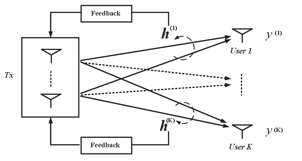
Refer to caption — Fig. 1: System model of $K$ -user MISO BC with CSIT feedback.

It is well known that the performance of the BC is greatly affected by the timeliness and quality of feedback; having full CSIT allows for the optimal $\min\{M,K\}$ sum degrees-of-freedom (DoF) (cf. [2])¹¹ 1 We remind the reader that for an achievable rate tuple $(R_{1},R_{2},\cdots,R_{K})$ , where $R_{i}$ is for user $i$ , the corresponding DoF tuple $(d_{1},d_{2},\cdots,d_{K})$ is given by $d_{i}=\lim_{P\to\infty}\frac{R_{i}}{\log P},\ i=1,2,\cdots,K$ . The corresponding DoF region ${\mathcal{D}}$ is then the set of all achievable DoF tuples $(d_{1},d_{2},\cdots,d_{K})$ ., while the absence of any CSIT reduces this to just $1$ sum DoF (cf. [3, 4]). This gap has spurred a plethora of works that seek to analyze and optimize BC communications in the presence of delayed and imperfect feedback. One of the works that stands out is the work by Maddah-Ali and Tse [5] which recently revealed the benefits of employing delayed CSIT over the BC, even if this CSIT is completely obsolete. Several interesting generalizations followed, including the work in [6] which showed that in the BC setting with $K=M+1$ , combining delayed CSIT with perfect (current) CSIT (over the last $\frac{K-1}{K}$ fraction of communication period) allows for the optimal sum DoF $M$ corresponding to full CSIT. A similar approach was exploited in [7] which revealed that, to achieve the maximum sum DoF $\min\{M,K\}$ , each user has to symmetrically feed back perfect CSIT over a $\frac{\min\{M,K\}}{K}$ fraction of the communication time, and that this fraction is optimal. Other interesting works in the context of utilizing delayed and current CSIT, can be found in [8, 9, 10, 11] which explored the setting of combining perfect delayed CSIT with immediately available imperfect CSIT, the work in [12, 13] which additionally considered the effects of the quality of delayed CSIT, the work in [14] which considered alternating CSIT feedback, the work in [15] which considered delayed and progressively evolving (progressively improving) current CSIT, and the works in [16, 17, 18, 19, 20, 21, 22] and many other publications.

Our work here generalizes many of the above settings, and seeks to establish fundamental tradeoff between DoF performance and CSIT feedback quality, over the general $K$ -user $M\times 1$ MISO BC.

I-A CSIT quantification and feedback model

We proceed to describe the quality and timeliness measure of CSIT feedback, and how this measure relates to existing work. We here use $\hat{\boldsymbol{h}}_{k,t}$ to denote the current channel estimate (for channel $\boldsymbol{h}_{k,t}$ ) at the transmitter at timeslot $t$ , and use

\tilde{\boldsymbol{h}}_{k,t}=\boldsymbol{h}_{k,t}-\hat{\boldsymbol{h}}_{k,t}

to denote the estimate error assumed to be mutually independent of $\hat{\boldsymbol{h}}_{k,t}$ and assumed to have i.i.d. Gaussian entries with power

\mathbb{E}\bigl[\|\tilde{\boldsymbol{h}}_{k,t}\|^{2}\bigr]\doteq P^{-\alpha_{k,t}},

for some CSI quality exponent $\alpha_{k,t}\in[0,1]$ describing the quality of this estimate. We note that $\alpha_{k,t}=0$ implies very little current CSIT knowledge, and that $\alpha_{k,t}=1$ implies perfect CSIT in terms of the DoF performance²² 2 This can be readily derived, using for example the work in [23]..

The approach extends over non-alternating CSIT settings in [5] and [8, 9, 10, 11], as well as over an alternating CSIT setting (cf. [14, 7]) where CSIT knowledge alternates between perfect CSIT ( $\alpha_{k,t}=1$ ), and delayed or no CSIT ( $\alpha_{k,t}=0$ ).

In a setting where communication takes place over $n$ such coherence periods ( $t=1,2,\cdots,n$ ), this approach offers a natural measure of a per-user average feedback cost, in the form of

\bar{\alpha}_{k}\defeq\frac{1}{n}\sum_{t=1}^{n}\alpha_{k,t},\quad k=1,2,\cdots,K,

as well as a measure of current CSIT feedback cost

\displaystyle\mathsf{C}_{\textrm{C}}\defeq\sum_{k=1}^{K}\bar{\alpha}_{k},

(2)

accumulated over all users.

I-A1 Alternating CSIT setting

In a setting where delayed CSIT is always available, the above model captures the alternating CSIT setting where the exponents are binary ( $\alpha_{k,t}=0,1$ ), in which case

\bar{\alpha}_{k}=\delta_{\textrm{P},k}

simply describes the fraction of time during which user $k$ feeds back perfect CSIT, with

\mathsf{C}_{\textrm{C}}=\mathsf{C}_{\textrm{P}}\defeq\sum_{k=1}^{K}\delta_{\textrm{P},k}

describing the total perfect CSIT feedback cost.

I-A2 Symmetric and asymmetric CSIT feedback

Motivated by the fact that different users might have different feedback capabilities due to the feedback channels with different capacities and different reliabilities, symmetric CSIT feedback ( $\bar{\alpha}_{1}=\cdots=\bar{\alpha}_{K}$ ) and asymmetric CSIT feedback ( $\bar{\alpha}_{k}\neq\bar{\alpha}_{k^{\prime}}\ \forall\,k\neq k^{{}^{\prime}}$ ) are considered in this work.

I-B Structure of the paper and Summary of Contributions

Section II provides the main results of this work:

•

In Theorem 1 we first provide a novel outer bound on the DoF region, for the $K$ -user $M\times 1$ MISO BC with partial current CSIT quantized with $\{\alpha_{k,t}\}_{k,t}$ , which bridges the case with no current CSIT (only delayed CSIT, or no CSIT) and the case with full CSIT. This result manages to generalize the results by Maddah-Ali and Tse ( $\alpha_{k,t}=0,\ \forall t,k$ ), Yang et al. and Gou and Jafar ( $K=2$ , $\alpha_{k,t}=\alpha,\ \forall t,k$ ), Maleki et al. ( $K=2$ , $\alpha_{1,t}=1,\alpha_{2,t}=0,\ \forall t$ ), Chen and Elia ( $K=2$ , $\alpha_{1,t}\neq\alpha_{2,t},\ \forall t$ ), Lee and Heath ( $M=K+1$ , $\alpha_{k,t}\in\{0,1\},\ \forall t,k$ ), and Tandon et al. ( $\alpha_{k,t}\in\{0,1\},\ \forall t,k$ ).
•

From Theorem 1, we then provide the upper bound on the sum DoF, which is tight for the case with $M\geq K$ (cf. Theorem 2) and the case with $M=2,K=3$ (cf. Theorem 3, Corollary 3a).
•

Furthermore, Theorem 4 characterizes the minimum total current CSIT feedback cost $\mathsf{C}_{\textrm{P}}^{\star}$ to achieve the maximum sum DoF, where the total feedback cost $\mathsf{C}_{\textrm{P}}^{\star}$ can be distributed among all the users with any (asymmetric and symmetric) combinations $\{\delta_{\textrm{P},k}\}_{k}$ .
•

In addition, the work considers some other general settings of BC and provides the DoF inner bound as a function of the CSIT feedback cost.

The main converse proof, that is for Theorem 1, is shown in the Section III and appendix. Most of the achievability proofs are shown in the Section IV. Finally Section V concludes the paper.

I-C Notation and conventions

Throughout this paper, we will consider communication over $n$ coherence periods where, for clarity of notation, we will focus on the case where we employ a single channel use per such coherence period (unit coherence period). Furthermore, unless stated otherwise, we assume perfect delayed CSIT, as well as adhere to the common convention (see [5, 24, 10, 9, 14, 7]), and assume perfect and global knowledge of channel state information at the receivers.

In terms of notation, $(\bullet)^{\scriptscriptstyle\mathsf{T}}$ , $(\bullet)^{{\scriptscriptstyle\mathsf{H}}}$ , $\text{tr}(\bullet)$ and $||\bullet||_{F}$ denote the transpose, conjugate transpose, trace and Frobenius norm of a matrix respectively, while $\mathrm{diag}(\bullet)$ denotes a diagonal matrix, $||\bullet||$ denotes the Euclidean norm, and $|\bullet|$ denotes either the magnitude of a scalar or the cardinality of a set. $o(\bullet)$ and $O(\bullet)$ come from the standard Landau notation, where $f(x)=o(g(x))$ implies $\lim_{x\to\infty}f(x)/g(x)=0$ . with $f(x)=O(g(x))$ implying that $\limsup_{x\to\infty}|f(x)/g(x)|<\infty$ . We also use $\doteq$ to denote exponential equality, i.e., we write $f(P)\doteq P^{B}$ to denote $\displaystyle\lim_{P\to\infty}\frac{\log f(P)}{\log P}=B$ . Similarly $\dotgeq$ and $\dotleq$ denote exponential inequalities. We use $\boldsymbol{A}\succeq\mathbf{0}$ to denote that $\boldsymbol{A}$ is positive semidefinite, and use $\boldsymbol{A}\preceq\boldsymbol{B}$ to mean that $\boldsymbol{B}-\boldsymbol{A}\succeq\mathbf{0}$ . Logarithms are of base $2$ .

II Main results

II-A Outer bounds

We first present the DoF region outer bound for the general $K$ -user $M\times 1$ MISO BC.

Theorem 1 (DoF region outer bound)

The DoF region of the $K$ -user $M\times 1$ MISO BC, is outer bounded as

	$\displaystyle\sum_{k=1}^{K}\!\frac{d_{\pi(k)}}{\min\{k,M\}}$	$\displaystyle\!\leq\!1\!+\!\sum_{k=1}^{K-1}\!\left(\frac{1}{\min\{k,M\}}\!-\!\frac{1}{\min\{K,M\}}\right)\bar{\alpha}_{\pi(k)}$		(3)
	$\displaystyle d_{k}$	$\displaystyle\leq 1,\quad k=1,2,\cdots,K$		(4)

where $\pi$ denotes a permutation of the ordered set $\{1,2,\cdots,K\}$ , and $\pi(k)$ denotes the $k$ th element of set $\pi$ .

Proof:

The proof is shown in Section III. ∎

Remark 1

It is noted that the bound captures the results in [5] ( $\alpha_{k,t}=0,\ \forall t,k$ ), in [9, 10] ( $K=2$ , $\alpha_{k,t}=\alpha,\ \forall t,k$ ), in [24] ( $M=K=2$ , $\alpha_{1,t}=1,\alpha_{2,t}=0,\ \forall\,t$ ), in [11] ( $K=2$ , $\alpha_{1,t}\neq\alpha_{2,t},\ \forall\,t$ ), in [14, 7] ( $\alpha_{k,t}\in\{0,1\},\ \forall t,k$ ), as well as in [25] ( $\alpha^{(k)}_{t}=\alpha,\ \forall t,k$ ).

Summing up the $K$ different bounds from the above, we directly have the following upper bound on the sum DoF $d_{\Sigma}\defeq\sum_{k=1}^{K}d_{k}$ , which is presented using the following notation

	$\displaystyle d_{\textrm{MAT}}$	$\displaystyle\defeq\frac{K}{1+\frac{1}{\min\{2,M\}}+\frac{1}{\min\{3,M\}}+\cdots+\frac{1}{\min\{K,M\}}}$		(5)
	$\displaystyle\Gamma$	$\displaystyle\defeq\frac{M}{\sum_{i=1}^{K-M}\frac{1}{i}(\frac{M-1}{M})^{i-1}+(\frac{M-1}{M})^{K-M}(\sum_{i=K-M+1}^{K}\frac{1}{i})}.$		(6)

Corollary 1a (Sum DoF outer bound)

For the $K$ -user $M\times 1$ MISO BC, the sum DoF is outer bounded as

\displaystyle d_{\Sigma}\leq d_{\textrm{MAT}}+\left(1-\frac{d_{\textrm{MAT}}}{\min\{K,M\}}\right)\sum_{k=1}^{K}\bar{\alpha}_{k}.

(7)

The above then readily translates onto a lower bound on the minimum possible total current CSIT feedback cost $\mathsf{C}_{\textrm{C}}=\sum_{k=1}^{K}\bar{\alpha}_{k}$ needed to achieve the maximum sum DoF³³ 3 Naturally the result is limited to the case where $\min\{K,M\}>1$ . $d_{\Sigma}=\min\{K,M\}$ .

Corollary 1b (Bound on CSIT cost for maximum DoF)

The minimum $\mathsf{C}_{\textrm{C}}$ required to achieve the maximum sum DoF $\min\{K,M\}$ of the $K$ -user $M\times 1$ MISO BC, is lower bounded as

\displaystyle\mathsf{C}_{\textrm{C}}^{\star}\geq\min\{K,M\}.

(8)

Transitioning to the alternating CSIT setting where $\alpha_{k,t}\in\{0,1\}$ , we have the following sum-DoF outer bound as a function of the perfect-CSIT duration $\bar{\alpha}_{k}=\delta_{\textrm{P},k}=\delta_{\textrm{P}},\ \forall\,k$ . We note that the bound holds irrespective of whether, in the remaining fraction of the time $1-\delta_{\textrm{P}}$ , the CSIT is delayed or non existent.

Corollary 1c (Outer bound, alternating CSIT)

For the $K$ -user $M\times 1$ MISO BC, the sum DoF is outer bounded as

\displaystyle d_{\Sigma}\leq d_{\textrm{MAT}}+\left(K-\frac{Kd_{\textrm{MAT}}}{\min\{K,M\}}\right)\min\left\{\delta_{\textrm{P}},\frac{\min\{K,M\}}{K}\right\}.

(9)

II-B Optimal cases of DoF characterizations

We now provide the optimal cases of DoF characterizations. The case with $M\geq K$ is first considered in the following.

Theorem 2 (Optimal case, $M\geq K$ )

For the $K$ -user $M\times 1$ MISO BC with $M\geq K$ , the optimal sum DoF is characterized as

\displaystyle d_{\Sigma}=(K-d_{\textrm{MAT}})\min\{\delta_{\textrm{P}},1\}+d_{\textrm{MAT}}.

(10)

Proof:

The converse and achievability proofs are derived from Corollary 1c and Proposition 2 (shown in the next subsection), respectively. ∎

Remark 2

It is noted that, for the special case with $M=K=2$ , the above characterization captures the result in [14].

Moving to the case where $M<K$ , we have the following optimal sum DoF characterizations for the case with $M=2,\ K=3$ . The first interest is placed on the minimum $\mathsf{C}_{\textrm{P}}^{\star}(d_{\Sigma})$ to achieve a sum DoF $d_{\Sigma}$ , recalling that $\mathsf{C}_{\textrm{P}}^{\star}=\sum_{k=1}^{K}\delta_{\textrm{P},k}$ describes the total perfect CSIT feedback cost.

Theorem 3 (Optimal case, $M=2,K=3$ )

For the three-user $2\times 1$ MISO BC, the minimum total perfect CSIT feedback cost is characterized as

\displaystyle\mathsf{C}_{\textrm{P}}^{\star}(d_{\Sigma})=(4d_{\Sigma}-6)^{+},\quad\forall\ d_{\Sigma}\in[0,2]

(11)

where the total feedback cost $\mathsf{C}_{\textrm{P}}^{\star}(d_{\Sigma})$ can be distributed among all the users with some combinations $\{\delta_{\textrm{P},k}\}_{k}$ such that $\delta_{\textrm{P},k}\leq\mathsf{C}_{\textrm{P}}^{\star}(d_{\Sigma})/2$ for any $k$ .

Proof:

The converse proof is directly from Corollary 1a, while the achievability proof is shown in Section IV-B. ∎

Theorem 3 reveals the fundamental tradeoff between sum DoF and total perfect CSIT feedback cost (see Fig 3). The following examples are provided to offer some insights corresponding to Theorem 3.

Example 1

For the target sum DoF $d_{\Sigma}=3/2,\ 7/4,\ 2$ , the minimum total perfect CSIT feedback cost is $\mathsf{C}_{\textrm{P}}^{\star}=0,\ 1,\ 2$ , respectively.

Example 2

The target $d_{\Sigma}=7/4$ is achievable with asymmetric feedback $\boldsymbol{\delta}_{\textrm{P}}=[1/6\quad 1/3\quad 1/2]$ , and symmetric feedback $\boldsymbol{\delta}_{\textrm{P}}=[1/3\quad 1/3\quad 1/3]$ , and some other feedback such that $\mathsf{C}_{\textrm{P}}^{\star}(7/4)=1$ .

Example 3

The target $d_{\Sigma}=2$ is achievable with asymmetric feedback $\boldsymbol{\delta}_{\textrm{P}}=[1/3\quad 2/3\quad 1]$ , and symmetric feedback $\boldsymbol{\delta}_{\textrm{P}}=[2/3\quad 2/3\quad 2/3]$ , and some other feedback such that $\mathsf{C}_{\textrm{P}}^{\star}(2)=2$ .

Transitioning to the symmetric setting where $\delta_{\textrm{P},k}=\delta_{\textrm{P}}\ \forall\,k$ , from Theorem 3 we have the fundamental tradeoff between optimal sum DoF and CSIT feedback cost $\delta_{\textrm{P}}$ .

Corollary 3a (Optimal case, $M=2,K=3$ , $\delta_{\textrm{P}}$ )

For the three-user $2\times 1$ MISO BC with symmetrically alternating CSIT feedback, the optimal sum DoF is characterized as

\displaystyle d_{\Sigma}=\min\left\{\frac{3(2+\delta_{\textrm{P}})}{4},2\right\}.

(12)

Now we address the questions of what is the minimum $\mathsf{C}_{\textrm{P}}^{\star}$ to achieve the maximum sum DoF $\min\{M,K\}$ for the general BC, and how to distribute $\mathsf{C}_{\textrm{P}}^{\star}$ among all the users, recalling again that $\mathsf{C}_{\textrm{P}}^{\star}$ is the total perfect CSIT feedback cost.

Theorem 4 (Minimum cost for maximum DoF)

For the $K$ -user $M\times 1$ MISO BC, the minimum total perfect CSIT feedback cost to achieve the maximum DoF is characterized as

\displaystyle\mathsf{C}_{\textrm{P}}^{\star}(\min\{M,K\})=\left\{\begin{array}[]{l l}0,&\text{if}\quad\min\{M,K\}=1\\ \min\{M,K\},&\text{if}\quad\min\{M,K\}>1\end{array}\right.

where the total feedback cost $\mathsf{C}_{\textrm{P}}^{\star}$ can be distributed among all the users with any combinations $\{\delta_{\textrm{P},k}\}_{k}$ .

Proof:

For the case with $\min\{M,K\}=1$ , simple TDMA is optimal in terms of the DoF performance. For the case with $\min\{M,K\}>1$ , the converse proof is directly derived from Corollary 1b, while the achievability proof is shown in Section IV-A. ∎

It is noted that Theorem 4 is a generalization of the result in [7] where only symmetric feedback was considered. The following examples are provided to offer some insights corresponding to Theorem 4.

Example 4

For the case where $M=2,\ K=4$ , the optimal 2 sum DoF performance is achievable, with asymmetric feedback $\boldsymbol{\delta}_{\textrm{P}}=[1/5\quad 2/5\quad 3/5\quad 4/5]$ , and symmetric feedback $\boldsymbol{\delta}_{\textrm{P}}=[1/2\quad 1/2\quad 1/2\quad 1/2]$ , and any other feedback such that $\mathsf{C}_{\textrm{P}}^{\star}=2$ .

Example 5

For the case where $M=3,\ K=5$ , the optimal 3 sum DoF performance is achievable, with asymmetric feedback $\boldsymbol{\delta}_{\textrm{P}}=[1/5\quad 2/5\quad 3/5\quad 4/5\quad 1]$ , and symmetric feedback $\boldsymbol{\delta}_{\textrm{P}}=[3/5\quad 3/5\quad 3/5\quad 3/5\quad 3/5]$ , and any other feedback such that $\mathsf{C}_{\textrm{P}}^{\star}=3$ .

The following corollary is derived from Theorem 4, where the case with $\min\{M,K\}>1$ is considered.

Corollary 4a (Minimum cost for maximum DoF)

For the $K$ -user $M\times 1$ MISO BC, where $J$ users instantaneously feed back perfect (current) CSIT, with the other users feeding back delayed CSIT, then the minimum number $J$ is $\min\{M,K\}$ , in order to achieve the maximum sum DoF $\min\{M,K\}$ .

II-C Inner bounds

In this subsection, we provide the following inner bounds on the sum DoF as a function of the CSIT cost, which are tight for many cases as stated.

Proposition 1 (Inner bound, $M=2,K\geq 3$ )

For the $K(\geq 3)$ -user $2\times 1$ MISO BC, the sum DoF is bounded as

\displaystyle d_{\Sigma}\geq\frac{3}{2}+\frac{K}{4}\min\{\delta_{\textrm{P}},\frac{2}{K}\}.

(16)

Proof:

The proof is shown in Section IV-C. ∎

Proposition 2 (Inner bound, $M\geq K$ and $M<K$ )

For the $K$ -user $M\times 1$ MISO BC, the sum DoF for the case with $M\geq K$ is bounded as

\displaystyle d_{\Sigma}\geq(K-d_{\textrm{MAT}})\min\{\delta_{\textrm{P}},1\}+d_{\textrm{MAT}},

(17)

while for the case with $M<K$ , the sum DoF is bounded as

\displaystyle d_{\Sigma}\geq(K-\frac{K\Gamma}{M})\min\{\delta_{\textrm{P}},\frac{M}{K}\}+\Gamma.

(18)

Proof:

The proof is shown in Section IV-D. ∎

Finally, we consider a case of BC with delayed CSIT feedback only, where $\delta_{\textrm{P}}=0$ . In this case, we use $\delta_{\textrm{D},k}$ to denote the fraction of time during which CSIT fed back from user $k$ is delayed, and focus on the case with $\delta_{\textrm{D},k}=\delta_{\textrm{D}},\ \forall k$ .

Proposition 3 (Inner bound on DoF with delayed CSIT)

For the $K(\geq 3)$ -user $2\times 1$ MISO BC, and for the case of $\delta_{\textrm{P}}=0$ , the sum DoF is bounded as

\displaystyle d_{\Sigma}\geq\min\left\{1+\frac{K}{2}\delta_{\textrm{D}},\ \frac{12}{11}+\frac{4K}{11}\delta_{\textrm{D}},\ \frac{3}{2}\right\}.

(19)

Proof:

The proof is shown in Section IV-E. ∎

Remark 3

For the $K$ -user MISO BC with current and delayed CSIT feedback, by increasing the number of users, the same DoF performance can be achievable with decreasing feedback cost per user. For example, for the $K$ -user MISO BC with $M=2$ , by increasing $K$ we can achieve any fixed DoF within the range of $(1,2]$ , with decreasing $\delta_{\textrm{P}}\leq\frac{2}{K}$ , and $\delta_{\textrm{D}}\leq\frac{9}{8K}$ , both of which approach to $0$ as $K$ is large.

III Converse proof of Theorem 1

We first provide the Proposition 4 to be used, where we drop the time index for simplicity.

Proposition 4

Let

	$\displaystyle y_{k}$	$\displaystyle=\boldsymbol{h}^{\scriptscriptstyle\mathsf{T}}_{k}\boldsymbol{x}+z_{k},$
	$\displaystyle\boldsymbol{y}_{k}$	$\displaystyle\triangleq[y_{1}\ y_{2}\ \cdots\ y_{k}]^{\scriptscriptstyle\mathsf{T}}$
	$\displaystyle\boldsymbol{z}_{k}$	$\displaystyle\triangleq[z_{1}\ z_{2}\ \cdots\ z_{k}]^{\scriptscriptstyle\mathsf{T}}$
	$\displaystyle\boldsymbol{H}_{k}$	$\displaystyle\triangleq[\boldsymbol{h}_{1}\ \boldsymbol{h}_{2}\ \cdots\ \boldsymbol{h}_{k}]^{\scriptscriptstyle\mathsf{T}}$
	$\displaystyle\boldsymbol{H}$	$\displaystyle\triangleq[\boldsymbol{h}_{1}\ \boldsymbol{h}_{2}\ \cdots\ \boldsymbol{h}_{K}]^{\scriptscriptstyle\mathsf{T}}$
	$\displaystyle\boldsymbol{H}$	$\displaystyle=\hat{\boldsymbol{H}}+\tilde{\boldsymbol{H}}$

where $\tilde{\boldsymbol{h}}_{i}\in\mathbb{C}^{M\times 1}$ has i.i.d. $\mathcal{N}_{\mathbb{C}}(0,\sigma^{2}_{i})$ entries. Then, for any $U$ such that $p_{X|U\hat{H}\tilde{H}}=p_{X|U\hat{H}}$ and $K\geq m\geq l$ , we have

l\,^{\prime}\,h(\boldsymbol{y}_{m}|U,\hat{H},\tilde{H})-m^{\prime}\,h(\boldsymbol{y}_{l}|U,\hat{H},\tilde{H})\leq-(m^{\prime}-l\,^{\prime})\sum_{i=1}^{l}\log\sigma^{2}_{i}+o(\log\mathsf{snr})

(20)

where we define $l\,^{\prime}\triangleq\min\left\{l,M\right\}$ and $m^{\prime}\triangleq\min\left\{m,M\right\}$ .

Proof:

The proof is shown in the Section VI. ∎

Now giving the observations and messages of users $1,\ldots,k-1$ to user $k$ , we establish the following genie-aided upper bounds on the achievable rates

$\displaystyle nR_{1}$	$\displaystyle\leq I(W_{1};y_{1}^{n}\,\|\,\Omega^{n})+n\epsilon$	(21)
$\displaystyle nR_{2}$	$\displaystyle\leq I(W_{2};y_{1}^{n},y_{2}^{n}\,\|\,W_{1},\Omega^{n})+n\epsilon$	(22)
	$\displaystyle\ \vdots$
$\displaystyle nR_{K}$	$\displaystyle\leq I(W_{K};y_{1}^{n},y_{2}^{n},\ldots,y_{K}^{n}\,\|\,W_{1},\ldots,W_{K-1},\Omega^{n})+n\epsilon$	(23)

where we apply Fano’s inequality and some basic chain rules of mutual information using the fact that messages from different users are independent, where we define

	$\displaystyle\boldsymbol{S}_{t}\defeq$	$\displaystyle\ \begin{bmatrix}\boldsymbol{h}_{1,t}\ \cdots\ \boldsymbol{h}_{K,t}\end{bmatrix}^{\scriptscriptstyle\mathsf{T}}$
	$\displaystyle\hat{\boldsymbol{S}}_{t}\defeq$	$\displaystyle\ \begin{bmatrix}\hat{\boldsymbol{h}}_{1,t}\ \cdots\ \hat{\boldsymbol{h}}_{K,t}\end{bmatrix}^{\scriptscriptstyle\mathsf{T}}$
	$\displaystyle\Omega^{n}\defeq$	$\displaystyle\ \{\boldsymbol{S}_{t},\hat{\boldsymbol{S}}_{t}\}_{t=1}^{n}$
	$\displaystyle y_{k}^{n}\defeq$	$\displaystyle\ \{y_{k,t}\}_{t=1}^{n}.$

Alternatively, we have

$\displaystyle nR_{1}$	$\displaystyle\leq h(y_{1}^{n}\,\|\,\Omega^{n})-h(y_{1}^{n}\,\|\,W_{1},\Omega^{n})+n\epsilon$	(24)
$\displaystyle nR_{2}$	$\displaystyle\leq h(y_{1}^{n},y_{2}^{n}\,\|\,W_{1},\Omega^{n})-h(y_{1}^{n},y_{2}^{n}\,\|\,W_{1},W_{2},\Omega^{n})+n\epsilon$	(25)
	$\displaystyle\ \vdots$
$\displaystyle nR_{K}$	$\displaystyle\leq h(y_{1}^{n},\ldots,y_{K}^{n}\,\|\,W_{1},\ldots,W_{K-1},\Omega^{n})-h(y_{1}^{n},\ldots,y_{K}^{n}\,\|\,W_{1},\ldots,W_{K},\Omega^{n})+n\epsilon.$	(26)

Therefore, it follows that

		$\displaystyle\sum_{k=1}^{K}\frac{n}{k^{\prime}}(R_{k}-\epsilon)$
		$\displaystyle\leq\sum_{k=1}^{K-1}\left(\frac{1}{(k+1)^{\prime}}h(y_{1}^{n},\ldots,y_{k+1}^{n}\,\|\,W_{1},\ldots,W_{k},\Omega^{n})-\frac{1}{k^{\prime}}h(y_{1}^{n},\ldots,y_{k}^{n}\,\|\,W_{1},\ldots,W_{k},\Omega^{n})\right)$
		$\displaystyle\qquad+h(y_{1}^{n}\,\|\,\Omega^{n})-\frac{1}{K^{\prime}}h(y_{1}^{n},\ldots,y_{K}^{n}\,\|\,W_{1},\ldots,W_{K},\Omega^{n})$		(27)
		$\displaystyle\leq\sum_{k=1}^{K-1}\sum_{t=1}^{n}\biggl(\frac{1}{(k+1)^{\prime}}h(y_{1,t},\ldots,y_{k+1,t}\,\|\,y_{1}^{t-1},\ldots,y_{k}^{t-1},W_{1},\ldots,W_{k},\Omega^{n})$
		$\displaystyle\qquad-\frac{1}{k^{\prime}}h(y_{1,t},\ldots,y_{k,t}\,\|\,y_{1}^{t-1},\ldots,y_{k}^{t-1},W_{1},\ldots,W_{k},\Omega^{n})\biggr)+n\log P+n\,o(\log P)$		(28)
		$\displaystyle\leq\log P\sum_{k=1}^{K-1}\sum_{t=1}^{n}\frac{(k+1)^{\prime}-k^{\prime}}{k^{\prime}(k+1)^{\prime}}\sum_{i=1}^{k}\alpha_{i,t}+n\log P+n\,o(\log P)$		(29)
		$\displaystyle=n\log P\sum_{k=1}^{K-1}\frac{(k+1)^{\prime}-k^{\prime}}{k^{\prime}(k+1)^{\prime}}\sum_{i=1}^{k}\bar{\alpha}_{i}+n\log P+n\,o(\log P)$		(30)
		$\displaystyle=n\log P\sum_{k=1}^{K-1}\Bigl(\frac{1}{k^{\prime}}-\frac{1}{K^{\prime}}\Bigr)\bar{\alpha}_{k}+n\log P+n\,o(\log P)$		(31)

where we define

\displaystyle k^{\prime}

\displaystyle\triangleq\min\left\{k,M\right\};

(32)

the inequality (28) is due to 1) the chain rule of differential entropy, 2) the fact that removing condition does not decrease differential entropy, 3) $h(y_{1,t}\,|\,\Omega^{n})\leq\log P+o(\log P)$ , i.e., Gaussian distribution maximizes differential entropy under covariance constraint, and 4) $h(y_{1}^{n},\ldots,y_{K}^{n}\,|\,W_{1},\ldots,W_{K},\Omega^{n})=h(z_{1,1},z_{1,2},\ldots,z_{K,n})>0$ ; (29) is from Proposition 4 by setting $U=\{y_{1}^{t-1},\ldots,y_{k}^{t-1},W_{1},\ldots,W_{k},\Omega^{n}\}\setminus\{\boldsymbol{S}_{t},\hat{\boldsymbol{S}}_{t}\}$ , ${H}={\boldsymbol{S}_{t}}$ , and $\hat{H}=\hat{\boldsymbol{S}_{t}}$ ; the last equality is obtained after putting the summation over $k$ inside the summation over $i$ and some basic manipulations. Similarly, we can interchange the roles of the users and obtain the same genie-aided bounds. Finally, the single antenna constraint gives that $d_{i}\leq 1,\ i=1,\cdots,K$ . With this, we complete the proof.

IV Details of achievability proofs

In this section, we provide the details of the achievability proofs. Specifically, the achievability proof of Theorem 4 is first described in Section IV-A, which can be applied in parts for the achievability proof of Theorem IV-B shown in Section IV-B, with the proposition proofs shown in the rest of this section.

IV-A Achievability proof of Theorem 4

We will prove that, the optimal sum DoF $d_{\Sigma}=\min\{M,K\}$ is achievable with any CSIT feedback cost $\boldsymbol{\delta}_{\textrm{P}}\defeq[\delta_{\textrm{P},1}\quad\delta_{\textrm{P},2}\quad\cdots\quad\delta_{\textrm{P},K}]\in\mathbb{R}^{K}$ such that $\mathsf{C}_{\textrm{P}}=\sum_{k=1}^{K}\delta_{\textrm{P},k}=\min\{M,K\}$ . First of all, we note that there exists a minimum number $n$ such that

\boldsymbol{\delta}_{\textrm{P}}^{\prime}\defeq[\delta_{\textrm{P},1}^{\prime}\quad\delta_{\textrm{P},2}^{\prime}\ \cdots\ \delta_{\textrm{P},K}^{\prime}]\defeq n\boldsymbol{\delta}_{\textrm{P}}=[n\delta_{\textrm{P},1}\quad n\delta_{\textrm{P},2}\ \cdots\ n\delta_{\textrm{P},K}]\in\mathbb{Z}^{K}

is an integer vector. The explicit communication with $n$ channel uses is given as follows:

•

Step 1: Initially set time index $t=1$ .
•

Step 2: Permute user indices orderly into a set ${\mathcal{U}}$ such that $\delta_{\textrm{P},{\mathcal{U}}(1)}^{\prime}\leq\delta_{\textrm{P},{\mathcal{U}}(2)}^{\prime}\leq\cdots\leq\delta_{\textrm{P},{\mathcal{U}}(K)}^{\prime}$ , where ${\mathcal{U}}(k)$ denotes the $k$ th element of set ${\mathcal{U}}$ , and where ${\mathcal{U}}(k)\in\{1,2,\cdots,K\}$ .
•

Step 3: Select $\min\{M,K\}$ users to communicate: users ${\mathcal{U}}(K-\min\{M,K\}+1),\cdots,{\mathcal{U}}(K-1),{\mathcal{U}}(K)$ .
•

Step 4: Let selected users feed back perfect CSIT at time $t$ , keeping the rest users silent.
•

Step 5: The transmitter sends $\min\{M,K\}$ independent symbols to those selected users respectively, which can be done with simple zero-forcing.
•

Step 6: Set $\delta_{\textrm{P},{\mathcal{U}}(k)}^{\prime}=\delta_{\textrm{P},{\mathcal{U}}(k)}^{\prime}-1,\ k=K-\min\{M,K\}+1,\cdots,K-1,K$ .
•

Step 7: Set $t=t+1$ . If renewed $t>n$ then terminate, else go back to step 2.

In the above communication with $n$ channel uses, the algorithm guarantees that user $i$ is selected by $\delta_{\textrm{P},k}^{\prime}=n\delta_{\textrm{P},k}$ times totally, and that $\min\{M,K\}$ different users are selected in each channel use. As a result, the optimal sum DoF $d_{\Sigma}=\min\{M,K\}$ is achievable.

Now we consider an example with $M=2,\ K=3$ , and $\boldsymbol{\delta}_{\textrm{P}}=[1/3\quad 2/3\quad 1]$ , and show that the optimal sum DoF $d_{\Sigma}=2$ is achievable with the following communication:

•

Let $n=3$ . Initially $\delta_{\textrm{P},1}^{\prime}=n\delta_{\textrm{P},1}=1$ , $\delta_{\textrm{P},2}^{\prime}=n\delta_{\textrm{P},2}=2$ , $\delta_{\textrm{P},3}^{\prime}=n\delta_{\textrm{P},3}=3$ .
•

For $t=1$ , we have ${\mathcal{U}}=\{1,2,3\}$ , and $\delta_{\textrm{P},{\mathcal{U}}(1)}^{\prime}=1$ , $\delta_{\textrm{P},{\mathcal{U}}(2)}^{\prime}=2$ , $\delta_{\textrm{P},{\mathcal{U}}(3)}^{\prime}=3$ . Users 3 and 2 are selected to communicate.
•

For $t=2$ , we update the parameters as ${\mathcal{U}}=\{1,2,3\}$ , and $\delta_{\textrm{P},{\mathcal{U}}(1)}^{\prime}=1$ , $\delta_{\textrm{P},{\mathcal{U}}(2)}^{\prime}=1$ , $\delta_{\textrm{P},{\mathcal{U}}(3)}^{\prime}=2$ . At this time, again user 3 and user 2 are selected to communicate.
•

For $t=3$ , we update the parameters as ${\mathcal{U}}=\{2,1,3\}$ , and $\delta_{\textrm{P},{\mathcal{U}}(1)}^{\prime}=0$ , $\delta_{\textrm{P},{\mathcal{U}}(2)}^{\prime}=1$ , $\delta_{\textrm{P},{\mathcal{U}}(3)}^{\prime}=1$ . At this time, user 3 and user 1 are selected to communicate. After that the communication terminates.

In the above communication with three channel uses, the transmitter sends two symbols in each channel use, which allows for the optimal sum DoF $d_{\Sigma}=2$ (see Table I).

TABLE I: Summary of the scheme for achieving

d^{*}_{\sum}=2

with

\mathsf{C}_{\textrm{P}}^{\star}=2

, where

M=2,\ K=3

\delta_{\textrm{P},1}=1/3,\ \delta_{\textrm{P},2}=2/3,\ \delta_{\textrm{P},3}=1

time $t$	1	2	3
${\mathcal{U}}$	$\{1,2,3\}$	$\{1,2,3\}$	$\{2,1,3\}$
$\{\delta_{\textrm{P},{\mathcal{U}}(1)}^{\prime},\ \delta_{\textrm{P},{\mathcal{U}}(2)}^{\prime},\ \delta_{\textrm{P},{\mathcal{U}}(3)}^{\prime}\}$	$\{1,2,3\}$	$\{1,1,2\}$	$\{0,1,1\}$
Active users	user 2, 3	user 2, 3	user 1, 3
Perfect CSIT feedback	user 3: yes	user 3: yes	user 3: yes
	user 2: yes	user 2: yes	user 2: no
	user 1: no	user 1: no	user 1: yes
No. of transmitted symbols	$2$	$2$	$2$

IV-B Achievability proof of Theorem 3

We proceed to show that, any sum DoF $d_{\Sigma}\in[3/2,2]$ is achievable with the feedback

\delta_{\textrm{P},k}\leq\frac{\mathsf{C}_{\textrm{P}}}{2},\ k=1,2,3,\quad\text{such that}\quad\mathsf{C}_{\textrm{P}}=\sum_{k=1}^{3}\delta_{\textrm{P},k}=4d_{\Sigma}-6.

First of all, we note that there exists a minimum number $n$ such that

[2n\delta_{\textrm{P},1}/\mathsf{C}_{\textrm{P}}\quad 2n\delta_{\textrm{P},2}/\mathsf{C}_{\textrm{P}}\quad n2\delta_{\textrm{P},3}/\mathsf{C}_{\textrm{P}}]\in\mathbb{Z}^{3},\quad\text{and}\quad 2n/\mathsf{C}_{\textrm{P}}\in\mathbb{Z}.

The scheme has two blocks, with the first block consisting of $n$ channel uses, and the second block consisting of

n^{{}^{\prime}}=2n/\mathsf{C}_{\textrm{P}}-n

channel uses. In the first block, we use the algorithm shown in the Section IV-A to achieve the full sum DoF in those $n$ channel uses, during which user $k$ feeds back perfect CSIT in $2n\delta_{\textrm{P},3}/\mathsf{C}_{\textrm{P}}$ channel uses, for $k=1,2,3$ . In the second block, we use the Maddah-Ali and Tse scheme in [5] to achieve 3/2 sum DoF in those $n^{{}^{\prime}}$ channel uses, during which each user feeds back delayed CSIT only.

The communication with $n$ channel uses for the first block is given as follows:

•

Step 1: Let $\delta_{\textrm{P},k}^{\prime}=2n\delta_{\textrm{P},k}/\mathsf{C}_{\textrm{P}}$ for all $k$ . Initially, set $t=1$ .
•

The steps 2, 3, 4, 5, 6 are the same as those in the algorithm shown in Section IV-A, for $M=2,K=3$ .
•

Step 7: Set $t=t+1$ . If renewed $t>n$ then terminate, else go back to step 2.

In the above communication with $n$ channel uses, the algorithm guarantees that user $k$ , $k=1,2,3,$ is selected by $\delta_{\textrm{P},k}^{\prime}=2n\delta_{\textrm{P},k}/\mathsf{C}_{\textrm{P}}$ times. We note that $\delta_{\textrm{P},k}^{\prime}\leq n$ under the constraint $\delta_{\textrm{P},k}\leq\mathsf{C}_{\textrm{P}}/2$ for any $k$ , and that $\sum^{K}_{k=1}\delta_{\textrm{P},k}^{\prime}=2n$ , to suggest that in each timeslot two different users are selected, which allows for the optimal $2$ sum DoF in this block.

As stated, in the second block, we use the MAT scheme to achieve the 3/2 sum DoF in those $n^{{}^{\prime}}$ channel uses, during which each user feeds back delayed CSIT only. As a result, in the total $n+n^{{}^{\prime}}$ channel uses communication, user $k=1,2,3$ feeds back perfect CSIT in $2n\delta_{\textrm{P},k}/(\mathsf{C}_{\textrm{P}}(n+n^{{}^{\prime}}))=\delta_{\textrm{P},k}$ fraction of communication period, with achievable sum DoF given as

d_{\Sigma}=\frac{2n}{(n+n^{{}^{\prime}})}+\frac{3n^{{}^{\prime}}}{2(n+n^{{}^{\prime}})}=\frac{3}{2}+\frac{1}{4}\mathsf{C}_{\textrm{P}}.

We note that the achievability scheme applies to the case of having some $\delta_{\textrm{P},1},\delta_{\textrm{P},2},\delta_{\textrm{P},3}\leq\mathsf{C}_{\textrm{P}}/2$ such that $\mathsf{C}_{\textrm{P}}=4d_{\Sigma}-6$ , and allows to achieve any sum DoF $d_{\Sigma}\in[3/2,2]$ . Apparently, $\mathsf{C}_{\textrm{P}}=0$ allows for any sum DoF $d_{\Sigma}\in[0,3/2]$ , which completes the proof.

IV-C Proof of Proposition 1

The achievability scheme is based on time sharing between two strategies of CSIT feedback, i.e., delayed CSIT feedback with $\delta_{\textrm{P}}^{\prime}=0$ and alternating CSIT feedback with $\delta_{\textrm{P}}^{\prime\prime}=\frac{2}{K}$ , where the first strategy achieves $d_{\Sigma}^{\prime}=3/2$ by applying Maddah-Ali and Tse (MAT) scheme (see in [5]), with the second strategy achieving $d_{\Sigma}^{\prime\prime}=2$ by using alternating CSIT feedback manner (see in [7]).

Let $\Delta\in[0,1]$ (res. $1-\Delta$ ) be the fraction of time during which the first (res. second) CSIT feedback strategy is used in the communication. As a result, the final feedback cost (per user) is given as

\displaystyle\delta_{\textrm{P}}=\delta_{\textrm{P}}^{\prime}\Delta+\delta_{\textrm{P}}^{\prime\prime}(1-\Delta),

(33)

implying that

\displaystyle\Delta=\frac{\delta_{\textrm{P}}^{\prime\prime}-\delta_{\textrm{P}}}{\delta_{\textrm{P}}^{\prime\prime}-\delta_{\textrm{P}}^{\prime}},

(34)

with final sum DoF given as

$\displaystyle d_{\Sigma}$	$\displaystyle=d_{\Sigma}^{\prime}\Delta+d_{\Sigma}^{\prime\prime}(1-\Delta)$
	$\displaystyle=d_{\Sigma}^{\prime\prime}+\Delta(d_{\Sigma}^{\prime}-d_{\Sigma}^{\prime\prime})$
	$\displaystyle=d_{\Sigma}^{\prime\prime}+(d_{\Sigma}^{\prime}-d_{\Sigma}^{\prime\prime})\frac{\delta_{\textrm{P}}^{\prime\prime}-\delta_{\textrm{P}}}{\delta_{\textrm{P}}^{\prime\prime}-\delta_{\textrm{P}}^{\prime}}$
	$\displaystyle=\frac{3}{2}+\frac{K}{4}\delta_{\textrm{P}}$	(35)

which completes the proof.

IV-D Proof of Proposition 2

For the case with $M\geq K$ , the proposed scheme is based on time sharing between delayed CSIT feedback with $\delta_{\textrm{P}}^{\prime}=0$ and full CSIT feedback with $\delta_{\textrm{P}}^{\prime\prime}=1$ , where the first feedback strategy achieves $d^{\ {}^{\prime}}_{\sum}=d_{\textrm{MAT}}$ by applying MAT scheme, with the second one achieving $d^{\ {}^{\prime\prime}}_{\sum}=K$ . As a result, following the steps in (33), (34), (35), the final sum DoF is calculated as

	$\displaystyle d_{\Sigma}$	$\displaystyle=d_{\Sigma}^{\prime\prime}+(d_{\Sigma}^{\prime}-d_{\Sigma}^{\prime\prime})\frac{\delta_{\textrm{P}}^{\prime\prime}-\delta_{\textrm{P}}}{\delta_{\textrm{P}}^{\prime\prime}-\delta_{\textrm{P}}^{\prime}}$
		$\displaystyle=(K-d_{\textrm{MAT}})\delta_{\textrm{P}}+d_{\textrm{MAT}}$

where $\delta_{\textrm{P}}\in[0,1]$ is the final feedback cost (per user) for this case.

Similar approach is exploited for the case with $M<K$ . In this case, we apply time sharing between delayed CSIT feedback with $\delta_{\textrm{P}}^{\prime}=0$ and alternating CSIT feedback with $\delta_{\textrm{P}}^{\prime\prime}=M/K$ . In this case, the first feedback strategy achieves $d_{\Sigma}^{\prime}=\Gamma$ by applying MAT scheme, with the second strategy achieving $d_{\Sigma}^{\prime\prime}=M$ by using alternating CSIT feedback manner. As a result, for $\delta_{\textrm{P}}\in[0,\frac{M}{K}]$ being the final feedback cost for this case, the final sum DoF is calculated as

	$\displaystyle d_{\Sigma}$	$\displaystyle=d_{\Sigma}^{\prime\prime}+(d_{\Sigma}^{\prime}-d_{\Sigma}^{\prime\prime})\frac{\delta_{\textrm{P}}^{\prime\prime}-\delta_{\textrm{P}}}{\delta_{\textrm{P}}^{\prime\prime}-\delta_{\textrm{P}}^{\prime}}$
		$\displaystyle=(K-\frac{K\Gamma}{M})\delta_{\textrm{P}}+\Gamma$

which completes the proof.

IV-E Proof of Proposition 3

As shown in the Fig 6, the sum DoF performance has three regions:

\displaystyle d_{\Sigma}=\left\{\begin{array}[]{l l}1+\frac{K}{2}\delta_{\textrm{D}},&\quad\delta_{\textrm{D}}\in[0,\frac{2}{3K}]\\ \frac{12}{11}+\frac{4K}{11}\delta_{\textrm{D}},&\quad\delta_{\textrm{D}}\in[\frac{2}{3K},\frac{9}{8K}]\\ 3/2,&\quad\delta_{\textrm{D}}\in[\frac{9}{8K},1].\end{array}\right.

In the following, we will prove that the sum DoF $d_{\Sigma}=1,\ \frac{4}{3},\ \frac{3}{2}$ are achievable with $\delta_{\textrm{D}}=0,\ \frac{2}{3K},\ \frac{9}{8K}$ , respectively. At the end, the whole DoF performance declared can be achievable by time sharing between those performance points.

The proposed scheme achieving $d_{\Sigma}=\frac{4}{3}$ with $\delta_{\textrm{D}}=\frac{2}{3K}$ , is a modified version of the MAT scheme in [5]. The new scheme has $K$ blocks, with each block consisting of three channel uses. In each block, four independent symbols are sent to two orderly selected users, which can be done with MAT scheme with each of two chosen user feeding back delayed CSIT in one channel use. As a result, $d_{\Sigma}=\frac{4}{3}$ is achievable with $\delta_{\textrm{D}}=\frac{2}{3K}$ , using the fact that each of $K$ users needs to feed back delayed CSIT twice only in the whole communication (see Table II).

TABLE II: Summary of the achievability scheme for achieving

d_{\Sigma}=\frac{4}{3}

with

\delta_{\textrm{D}}=\frac{2}{3K}

block index	1	2	3	$\cdots$	$K$
No. of channel uses	3	3	3	$\cdots$	3
Active users	user 1, 2	user 2, 3	user 3, 4	$\cdots$	user $K$ , 1
Delayed CSIT feedback	user 1: $1/3$	user 2: $1/3$	user 3: $1/3$	$\cdots$	user $K$ : $1/3$
fraction in a block	user 2: $1/3$	user 3: $1/3$	user 4: $1/3$		user 1: $1/3$
	the rest: 0	the rest: 0	the rest: 0		the rest: 0
Sum DoF	$4/3$	$4/3$	$4/3$	$\cdots$	$4/3$
in a block

Similarly, the proposed scheme achieving $d_{\Sigma}=\frac{3}{2}$ with $\delta_{\textrm{D}}=\frac{9}{8K}$ has $K$ blocks, with each block consisting of 8 channel uses. In each block, 3 out of $K$ users are selected to communicate. In this case, $12$ independent symbols are sent to the chosen users during each block, which can be done with another MAT scheme with each of chosen users feeding back delayed CSIT in 3 channel uses. As a result, $d_{\Sigma}=\frac{3}{2}$ is achievable with $\delta_{\textrm{D}}=\frac{9}{8K}$ , using the fact that each of $K$ users needs to feed back delayed CSIT 9 times only in the whole communication (see Table III).

Finally, $d_{\Sigma}=1$ is achievable without any CSIT. By now, we complete the proof.

TABLE III: Summary of the achievability scheme for achieving

d_{\Sigma}=\frac{3}{2}

with

\delta_{\textrm{D}}=\frac{9}{8K}

block index	1	2	3	$\cdots$	$K$
No. of channel uses	8	8	8	$\cdots$	8
Active users	user 1, 2, 3	user 2, 3, 4	user 3, 4, 5	$\cdots$	user $K$ , 1, 2
Delayed CSIT feedback	user 1: $3/8$	user 2: $3/8$	user 3: $3/8$	$\cdots$	user $K$ : $3/8$
fraction in a block	user 2: $3/8$	user 3: $3/8$	user 4: $3/8$		user 1: $3/8$
	user 3: $3/8$	user 4: $3/8$	user 5: $3/8$		user 2: $3/8$
	the rest: 0	the rest: 0	the rest: 0		the rest: 0
Sum DoF	$3/2$	$3/2$	$3/2$	$\cdots$	$3/2$
in a block

V Conclusions

This work considered the general multiuser MISO BC, and established inner and outer bounds on the tradeoff between DoF performance and CSIT feedback quality, which are optimal for many cases. Those bounds, as well as some analysis, were provided with the aim of giving insights on how much CSIT feedback to achieve a certain DoF performance.

VI Appendix - Proof details of Proposition 4

In the following, we will prove Proposition 4 used for the converse proof, as well as three lemmas to be used here.

Lemma 1

⁴⁴ 4 We note that Lemma 1 is a slightly more general version of the result in [26, Lemma 6].

Let $\boldsymbol{G}=\hat{\boldsymbol{G}}+\tilde{\boldsymbol{G}}\in\mathbb{C}^{m\times m}$ where $\tilde{\boldsymbol{G}}$ has i.i.d. $\mathcal{N}_{c}(0,1)$ entries, and $\tilde{\boldsymbol{G}}$ is independent of $\hat{\boldsymbol{G}}$ . Then, we have

\displaystyle\mathbb{E}_{\tilde{G}}\bigl[\log\det\left(\boldsymbol{G}^{\scriptscriptstyle\mathsf{H}}\boldsymbol{G}\right)\bigr]=\sum_{i=1}^{\tau}\log\bigl(\lambda_{i}(\hat{\boldsymbol{G}}^{\scriptscriptstyle\mathsf{H}}\hat{\boldsymbol{G}})\bigr)+o(\log\mathsf{snr})

(40)

where $\lambda_{i}(\hat{\boldsymbol{G}}^{\scriptscriptstyle\mathsf{H}}\hat{\boldsymbol{G}})$ denotes the $i$ th largest eigenvalue of $\hat{\boldsymbol{G}}^{\scriptscriptstyle\mathsf{H}}\hat{\boldsymbol{G}}$ ; $\tau$ is the number of eigenvalues of $\hat{\boldsymbol{G}}^{\scriptscriptstyle\mathsf{H}}\hat{\boldsymbol{G}}$ that do not vanish with $\mathsf{snr}$ , i.e., $\lambda_{i}(\hat{\boldsymbol{G}}^{\scriptscriptstyle\mathsf{H}}\hat{\boldsymbol{G}})=o(1)$ when $\mathsf{snr}$ is large, $\forall\,i>\tau$ .

Lemma 2

For $\boldsymbol{P}\in\mathbb{C}^{m\times m}$ a permutation matrix and $\boldsymbol{A}\in\mathbb{C}^{m\times m}$ , let $\boldsymbol{A}\boldsymbol{P}=\boldsymbol{Q}\boldsymbol{R}$ be the QR decomposition of the column permuted version of $\boldsymbol{A}$ . Then, there exist at least one permutation matrix $\boldsymbol{P}$ such that

\displaystyle r_{ii}^{2}

\displaystyle\geq\frac{1}{{m-i+1}}\lambda_{i}(\boldsymbol{A}^{\scriptscriptstyle\mathsf{H}}\boldsymbol{A}),\quad i=1,\ldots,m

(41)

where as stated $\lambda_{i}(\boldsymbol{A}^{\scriptscriptstyle\mathsf{H}}\boldsymbol{A})$ is the $i$ th largest eigenvalue of $\boldsymbol{A}^{\scriptscriptstyle\mathsf{H}}\boldsymbol{A}$ ; $r_{ii}$ is the $i$ th diagonal elements of $\boldsymbol{R}$ .

Lemma 3

For any matrix $\boldsymbol{A}\in\mathbb{C}^{m\times m}$ , there exists a column permuted version $\bar{\boldsymbol{A}}$ , such that

\displaystyle\det(\bar{\boldsymbol{A}}_{\mathcal{I}}^{\scriptscriptstyle\mathsf{H}}\bar{\boldsymbol{A}}_{\mathcal{I}})

\displaystyle\geq m^{-|\mathcal{I}|}\prod_{i\in\mathcal{I}}\lambda_{i}(\boldsymbol{A}^{\scriptscriptstyle\mathsf{H}}\boldsymbol{A}),\quad\forall\,\mathcal{I}\subseteq\left\{1,\ldots,m\right\}

(42)

where $\bar{\boldsymbol{A}}_{\mathcal{I}}=[A_{ji}:\ j\in\left\{1,\ldots,m\right\},\,i\in\mathcal{I}]\in\mathbb{C}^{m\times|\mathcal{I}|}$ is the submatrix of $\boldsymbol{A}$ formed by the columns with indices in $\mathcal{I}$ .

VI-A Proof of Lemma 1

Let us perform a singular value decomposition (SVD) on the matrix $\hat{\boldsymbol{G}}$ , i.e., $\hat{\boldsymbol{G}}=\boldsymbol{U}\left[\begin{smallmatrix}\boldsymbol{D}_{1}&\\ &\boldsymbol{D}_{2}\end{smallmatrix}\right]\boldsymbol{V}^{\scriptscriptstyle\mathsf{H}}$ where $\boldsymbol{U},\boldsymbol{V}\in\mathbb{C}^{m\times m}$ are unitary matrices and $\boldsymbol{D}_{1}$ and $\boldsymbol{D}_{2}$ are $\tau^{\prime}\times\tau^{\prime}$ and $(m-\tau^{\prime})\times(m-\tau^{\prime})$ diagonal matrices of the singular values of $\hat{\boldsymbol{G}}$ . Without loss of generality, we assume that the $i$ th singluar value, $i=1,\ldots,m$ , scales with $\mathsf{snr}$ as $\mathsf{snr}^{b_{i}}$ , when $\mathsf{snr}$ is large. Moreover, the singular values in $\boldsymbol{D}_{1}$ are such that $b_{i}>0$ and those in $\boldsymbol{D}_{2}$ verify $b_{i}\leq 0$ . First, we have the following lower bound

		$\displaystyle\mathbb{E}_{\tilde{G}}\bigl[\log\det\left(\boldsymbol{G}^{\scriptscriptstyle\mathsf{H}}\boldsymbol{G}\right)\bigr]$
		$\displaystyle=\mathbb{E}_{\boldsymbol{M}}\biggl[\log\det\left(\left(\left[\begin{smallmatrix}\boldsymbol{D}_{1}&\\ &\boldsymbol{D}_{2}\end{smallmatrix}\right]+\boldsymbol{M}\right)^{\scriptscriptstyle\mathsf{H}}\left(\left[\begin{smallmatrix}\boldsymbol{D}_{1}&\\ &\boldsymbol{D}_{2}\end{smallmatrix}\right]+\boldsymbol{M}\right)\right)\biggr]$		(43)
		$\displaystyle\geq\mathbb{E}_{\boldsymbol{M}}\biggl[\log\det\left(\left(\left[\begin{smallmatrix}\boldsymbol{D}_{1}&\\ &0\end{smallmatrix}\right]+\boldsymbol{M}\right)^{\scriptscriptstyle\mathsf{H}}\left(\left[\begin{smallmatrix}\boldsymbol{D}_{1}&\\ &0\end{smallmatrix}\right]+\boldsymbol{M}\right)\right)\biggr]$		(44)
		$\displaystyle=\mathbb{E}_{\boldsymbol{M}}\Bigl[\log\bigl\lvert\det\left(\boldsymbol{D}_{1}+\boldsymbol{M}_{11}\right)\det\bigl(\boldsymbol{M}_{22}-\underbrace{\boldsymbol{M}_{21}\left(\boldsymbol{D}_{1}+\boldsymbol{M}_{11}\right)^{-1}}_{\boldsymbol{B}}\boldsymbol{M}_{12}\bigr)\bigr\rvert^{2}\Bigr]$		(45)
		$\displaystyle=\log\bigl\lvert\det\left(\boldsymbol{D}_{1}\right)\bigr\rvert^{2}+\mathbb{E}_{\boldsymbol{M}_{11}}\Bigl[\log\bigl\lvert\det\left(I+\boldsymbol{D}_{1}^{-1}\boldsymbol{M}_{11}\right)\bigr\rvert^{2}\Bigr]+\mathbb{E}_{\boldsymbol{B}}\mathbb{E}_{\tilde{\boldsymbol{M}}}\bigl[\log\det(\tilde{\boldsymbol{M}}^{H}(I+\boldsymbol{B}\boldsymbol{B}^{H})\tilde{\boldsymbol{M}})\bigr]$		(46)
		$\displaystyle\geq\log\bigl\lvert\det\left(\boldsymbol{D}_{1}\right)\bigr\rvert^{2}+\mathbb{E}_{\boldsymbol{M}_{11}}\Bigl[\log\bigl\lvert\det\left(I+\boldsymbol{D}_{1}^{-1}\boldsymbol{M}_{11}\right)\bigr\rvert^{2}\Bigr]+\underbrace{\mathbb{E}_{\tilde{\boldsymbol{M}}}\bigl[\log\det(\tilde{\boldsymbol{M}}^{H}\tilde{\boldsymbol{M}})\bigr]}_{(\ln 2)^{-1}\sum_{l=0}^{m-\tau^{\prime}-1}\psi(m-\tau^{\prime}-l)=O(1)}$		(47)

where we define $\boldsymbol{M}\triangleq\boldsymbol{U}^{\scriptscriptstyle\mathsf{H}}\tilde{\boldsymbol{G}}\boldsymbol{V}=\left[\begin{smallmatrix}\boldsymbol{M}_{11}&\boldsymbol{M}_{12}\\ \boldsymbol{M}_{21}&\boldsymbol{M}_{22}\end{smallmatrix}\right]$ with $\boldsymbol{M}_{11}\in\mathbb{C}^{\tau^{\prime}\times\tau^{\prime}}$ , and remind that the entries of $\boldsymbol{M}$ , thus of $\boldsymbol{M}_{ij}$ , $i,j=1,2$ , are also i.i.d. $\mathcal{N}_{c}(0,1)$ ; (44) is from the fact that expectation of the log determinant of a non-central Wishart matrix is non-decreasing with in the “line-of-sight” component [27]; (45) is due to the identity $\det\left(\left[\begin{smallmatrix}\boldsymbol{N}_{11}&\boldsymbol{N}_{12}\\ \boldsymbol{N}_{21}&\boldsymbol{N}_{22}\end{smallmatrix}\right]\right)=\det(\boldsymbol{N}_{11})\det(\boldsymbol{N}_{22}-\boldsymbol{N}_{21}\boldsymbol{N}_{11}^{-1}\boldsymbol{N}_{12})$ whenever $\boldsymbol{N}_{11}$ is square and invertible; in (46), we notice that, given the matrix $\boldsymbol{B}\defeq\boldsymbol{M}_{21}\left(\boldsymbol{D}_{1}+\boldsymbol{M}_{11}\right)^{-1}$ , the columns of $\boldsymbol{M}_{22}-\boldsymbol{B}\boldsymbol{M}_{12}$ are i.i.d. $\mathcal{N}_{c}(0,I+\boldsymbol{B}\boldsymbol{B}^{H})$ , from which $\lvert\det(\boldsymbol{M}_{22}-\boldsymbol{B}\boldsymbol{M}_{12})\rvert^{2}$ is equivalent in distribution to $\det(\tilde{\boldsymbol{M}}^{H}(I+\boldsymbol{B}\boldsymbol{B}^{H})\tilde{\boldsymbol{M}})$ where $\tilde{\boldsymbol{M}}\in\mathbb{C}^{(m-\tau^{\prime})\times(m-\tau^{\prime})}$ has i.i.d. $\mathcal{N}_{c}(0,1)$ entries; the last inequality is from $\tilde{\boldsymbol{M}}^{H}(I+\boldsymbol{B}\boldsymbol{B}^{H})\tilde{\boldsymbol{M}}\succeq\tilde{\boldsymbol{M}}^{H}\tilde{\boldsymbol{M}}$ and therefore $\det(\tilde{\boldsymbol{M}}^{H}(I+\boldsymbol{B}\boldsymbol{B}^{H})\tilde{\boldsymbol{M}})\geq\det(\tilde{\boldsymbol{M}}^{H}\tilde{\boldsymbol{M}})$ , $\forall\,\boldsymbol{B}$ ; the closed-form term in the last inequality is due to [28] with $\psi(\cdot)$ being Euler’s digamma function. In the following, we show that $\mathbb{E}\bigl[\log\bigl\lvert\det\left(I+\boldsymbol{D}_{1}^{-1}\boldsymbol{M}_{11}\right)\bigr\rvert^{2}\bigr]\geq O(1)$ as well. To that end, we use the fact that the distribution of $\boldsymbol{M}_{11}$ is invariant to rotation, and so for $\boldsymbol{D}_{1}^{-1}\boldsymbol{M}_{11}$ . Specifically, introducing $\theta\sim\textrm{Unif}(0,2\pi]$ that is independent of the rest of the random variables, we have

$\displaystyle\mathbb{E}_{\boldsymbol{M}_{11}}\Bigl[\log\bigl\lvert\det\left(I+\boldsymbol{D}_{1}^{-1}\boldsymbol{M}_{11}\right)\bigr\rvert^{2}\Bigr]$	$\displaystyle=\mathbb{E}_{\boldsymbol{M}_{11},\theta}\Bigl[\log\bigl\lvert\det\left(I+\boldsymbol{D}_{1}^{-1}\boldsymbol{M}_{11}e^{j\theta}\right)\bigr\rvert^{2}\Bigr]$	(48)
	$\displaystyle=\mathbb{E}_{\boldsymbol{M}_{11},\theta}\Bigl[\log\bigl\lvert\det\left(e^{-j\theta}I+\boldsymbol{D}_{1}^{-1}\boldsymbol{M}_{11}\right)\bigr\rvert^{2}\Bigr]$	(49)
	$\displaystyle=\sum_{i=1}^{\tau^{\prime}}\mathbb{E}_{J}\mathbb{E}_{\theta}\bigl[\log\lvert e^{-j\theta}+\underbrace{\lambda_{i}(\boldsymbol{D}^{-1}\boldsymbol{M}_{11})}_{J_{i}}\rvert^{2}\bigr]$	(50)
	$\displaystyle=\sum_{i=1}^{\tau^{\prime}}\mathbb{E}_{J}\mathbb{E}_{\theta}[\log(1+\lvert{J_{i}}\rvert^{2}+2\lvert{J_{i}}\rvert\cos(\theta+\phi(J_{i})))]$	(51)
	$\displaystyle=\sum_{i=1}^{\tau^{\prime}}\mathbb{E}_{J}\mathbb{E}_{\theta}[\log(1+\lvert{J_{i}}\rvert^{2}+2\lvert{J_{i}}\rvert\cos(\theta))]$	(52)
	$\displaystyle\geq\sum_{i=1}^{\tau^{\prime}}\bigl[\mathbb{E}_{J}\bigl(\log(1+\lvert{J_{i}}\rvert^{2})\bigr)-1\bigr]$	(53)
	$\displaystyle\geq-\tau^{\prime}$	(54)

where the first equality is from the fact that $\boldsymbol{M}_{11}$ is equivalent to $\boldsymbol{M}_{11}e^{j\theta}$ as long as $\theta$ is independent of $\boldsymbol{M}_{11}$ and that $\boldsymbol{M}_{11}$ has independent circularly symmetric Gaussian entries; (50) is due to the characteristic polynomial of the matrix $-\boldsymbol{D}^{-1}\boldsymbol{M}_{11}$ ; in (51) we define $\phi(J_{i})$ the argument of $J_{i}$ that is independent of $\theta$ ; (52) is from the fact that $\mathrm{mod}(\theta+\phi)_{2\pi}\sim\textrm{Unif}(0,2\pi]$ and is independent of $\phi$ , as long as $\theta\sim\textrm{Unif}(0,2\pi]$ and is independent of $\phi$ , also known as the Crypto Lemma [29]; (53) is from the identity $\int_{0}^{1}\log(a+b\cos(2\pi t))\,\mathrm{d}t=\log\frac{a+\sqrt{a^{2}-b^{2}}}{2}\geq\log(a)-1$ , $\forall\,a\geq b>0$ . Combining (47) and (54), we have the lower bound

\displaystyle\mathbb{E}_{\tilde{G}}\bigl[\log\det\left(\boldsymbol{G}^{\scriptscriptstyle\mathsf{H}}\boldsymbol{G}\right)\bigr]\geq\log\bigl\lvert\det\left(\boldsymbol{D}_{1}\right)\bigr\rvert^{2}+O(1)

(55)

when $\mathsf{snr}$ is large. In fact, it has been shown that the $O(1)$ term here, sum of the $O(1)$ term in (47) and $-\tau^{\prime}$ in (54), does not depend on $\mathsf{snr}$ at all.

The next step is to derive an upper bound on $\mathbb{E}\bigl[\log\det\left(\boldsymbol{G}^{\scriptscriptstyle\mathsf{H}}\boldsymbol{G}\right)\bigr]$ . Following Jensen’s inequality, we have

$\displaystyle\mathbb{E}_{\tilde{G}}\bigl[\log\det(\boldsymbol{G}^{\scriptscriptstyle\mathsf{H}}\boldsymbol{G})\bigr]$	$\displaystyle\leq\log\det\bigl(\mathbb{E}_{\tilde{G}}[\boldsymbol{G}^{\scriptscriptstyle\mathsf{H}}\boldsymbol{G}]\bigr)$	(56)
	$\displaystyle=\log\det\left(\left[\begin{smallmatrix}\boldsymbol{D}_{1}^{2}&\\ &\boldsymbol{D}_{2}^{2}\end{smallmatrix}\right]+\mathbb{E}[\boldsymbol{M}^{\scriptscriptstyle\mathsf{H}}\boldsymbol{M}]\right)$	(57)
	$\displaystyle=\log\lvert\det\left(\boldsymbol{D}_{1}\right)\rvert^{2}+\underbrace{\log\det\left(I+m\boldsymbol{D}_{1}^{-2}\right)}_{o(1)}+\underbrace{\log\det\left(mI+\boldsymbol{D}_{2}^{2}\right)}_{o(\log\mathsf{snr})}$	(58)
	$\displaystyle=\log\lvert\det\left(\boldsymbol{D}_{1}\right)\rvert^{2}+o(\log\mathsf{snr})$	(59)

Putting the lower and upper bounds together, we have $\mathbb{E}\bigl[\log\det\left(\boldsymbol{G}^{\scriptscriptstyle\mathsf{H}}\boldsymbol{G}\right)\bigr]=\log\lvert\det\left(\boldsymbol{D}_{1}\right)\rvert^{2}+o(\log\mathsf{snr})$ . Finally, note that, since $\lambda_{i}(\hat{\boldsymbol{G}}^{\scriptscriptstyle\mathsf{H}}\hat{\boldsymbol{G}})\doteq\mathsf{snr}^{0}$ , $i=\tau^{\prime}+1,\ldots,\tau$ , we have

$\displaystyle\log\bigl\lvert\det\left(\boldsymbol{D}_{1}\right)\bigr\rvert^{2}$	$\displaystyle=\sum_{i=1}^{\tau^{\prime}}\log\bigl(\lambda_{i}(\hat{\boldsymbol{G}}^{\scriptscriptstyle\mathsf{H}}\hat{\boldsymbol{G}})\bigr)$	(60)
	$\displaystyle=\sum_{i=1}^{\tau}\log\bigl(\lambda_{i}(\hat{\boldsymbol{G}}^{\scriptscriptstyle\mathsf{H}}\hat{\boldsymbol{G}})\bigr)-\sum_{i=\tau^{\prime}+1}^{\tau}\log\bigl(\lambda_{i}(\hat{\boldsymbol{G}}^{\scriptscriptstyle\mathsf{H}}\hat{\boldsymbol{G}})\bigr)$	(61)
	$\displaystyle=\sum_{i=1}^{\tau}\log\bigl(\lambda_{i}(\hat{\boldsymbol{G}}^{\scriptscriptstyle\mathsf{H}}\hat{\boldsymbol{G}})\bigr)+o(\log\mathsf{snr})$	(62)

from which the proof is complete.

VI-B Proof of Lemma 2

The existence is proved by construction. Let $\boldsymbol{a}_{j}$ , $j=1,\ldots,m$ , be the $j$ th column of $\boldsymbol{A}$ . We define $j_{1}^{*}$ as the index of the column that has the largest Euclidean norm, i.e.,

\displaystyle j_{1}^{*}

\displaystyle=\arg\max_{j=1,\ldots,m}\|\boldsymbol{a}_{j}\|.

(63)

Swapping the $j_{1}^{*}$ and the first column, and denoting $\boldsymbol{A}_{1}=\boldsymbol{A}$ , we have

\displaystyle\boldsymbol{B}_{1}

\displaystyle\triangleq\boldsymbol{A}_{1}\boldsymbol{T}_{1,j_{1}^{*}}

(64)

where $\boldsymbol{T}_{ij}\in\mathbb{C}^{m\times m}$ denotes the permutation matrix that swaps the $i$ th and $j$ th columns. Now, let $\boldsymbol{U}_{1}\in\mathbb{C}^{m\times m}$ be any unitary matrix such that the first column is aligned with the first column of $\boldsymbol{B}_{1}$ , i.e., equal to $\frac{\boldsymbol{a}_{j_{1}^{*}}}{\|\boldsymbol{a}_{j_{1}^{*}}\|}$ . Then, we can construct a block-upper-triangular matrix $\boldsymbol{R}_{1}=\boldsymbol{U}_{1}^{\scriptscriptstyle\mathsf{H}}\boldsymbol{B}_{1}=\boldsymbol{U}_{1}^{\scriptscriptstyle\mathsf{H}}\boldsymbol{A}_{1}\boldsymbol{T}_{1,j_{1}^{*}}$ with the following form

\displaystyle\boldsymbol{R}_{1}

\displaystyle=\begin{bmatrix}r_{11}&*\\ \mathbf{0}_{(m-1)\times 1}&\boldsymbol{A}_{2}\end{bmatrix}

(65)

where it is readily shown that

$\displaystyle r_{11}^{2}$	$\displaystyle=\\|\boldsymbol{a}_{j_{1}^{*}}\\|^{2}$	(66)
	$\displaystyle\geq\frac{1}{m}\|\|\boldsymbol{A}_{1}\|\|^{2}_{F}$	(67)
	$\displaystyle\geq\frac{1}{m}\lambda_{1}(\boldsymbol{A}_{1}^{\scriptscriptstyle\mathsf{H}}\boldsymbol{A}_{1}).$	(68)

Repeating the same procedure on $\boldsymbol{A}_{2}$ , we will have $\boldsymbol{R}_{2}=\boldsymbol{U}_{2}^{\scriptscriptstyle\mathsf{H}}\boldsymbol{B}_{2}=\boldsymbol{U}_{2}^{\scriptscriptstyle\mathsf{H}}\boldsymbol{A}_{2}\boldsymbol{T}_{2,j_{2}^{*}}$ where all the involved matrices are similarly defined as above except for the reduced dimension $(m-1)\times(m-1)$ and

\displaystyle\boldsymbol{R}_{2}

\displaystyle=\begin{bmatrix}r_{22}&*\\ \mathbf{0}_{(m-2)\times 1}&\boldsymbol{A}_{3}\end{bmatrix}

(69)

where it is readily shown that

	$\displaystyle r_{22}^{2}$	$\displaystyle\geq\frac{1}{m-1}\lambda_{1}(\boldsymbol{A}_{2}^{\scriptscriptstyle\mathsf{H}}\boldsymbol{A}_{2})$		(70)
		$\displaystyle\geq\frac{1}{m-1}\lambda_{2}(\boldsymbol{A}_{1}^{\scriptscriptstyle\mathsf{H}}\boldsymbol{A}_{1}).$		(71)

Here, the last inequality is from the fact that, for any matrix $\boldsymbol{C}$ and a submatrix $\boldsymbol{C}_{k}$ by removing $k$ rows or columns, we have [30, Corollary 3.1.3]

\displaystyle\lambda_{i}(\boldsymbol{C}_{k}^{\scriptscriptstyle\mathsf{H}}\boldsymbol{C}_{k})\geq\lambda_{i+k}(\boldsymbol{C}^{\scriptscriptstyle\mathsf{H}}\boldsymbol{C})

(72)

where we recall that $\lambda_{i}$ is the $i$ th largest eigenvalue. Let us continue the procedure on $\boldsymbol{A}_{3}$ and so on. At the end, we will have all the $\left\{\boldsymbol{U}_{i}\right\}$ and $\left\{\boldsymbol{T}_{i,j_{i}^{*}}\right\}$ such that

\displaystyle\underbrace{\left[\begin{smallmatrix}I_{m-1}&\\ &\boldsymbol{U}_{m}^{\scriptscriptstyle\mathsf{H}}\end{smallmatrix}\right]\cdots\left[\begin{smallmatrix}I_{2}&\\ &\boldsymbol{U}_{3}^{\scriptscriptstyle\mathsf{H}}\end{smallmatrix}\right]\left[\begin{smallmatrix}1&\\ &\boldsymbol{U}_{2}^{\scriptscriptstyle\mathsf{H}}\end{smallmatrix}\right]\boldsymbol{U}_{1}^{\scriptscriptstyle\mathsf{H}}}_{\boldsymbol{Q}^{\scriptscriptstyle\mathsf{H}}}\boldsymbol{A}\underbrace{\boldsymbol{T}_{1,j_{1}^{*}}\left[\begin{smallmatrix}1&\\ &\boldsymbol{T}_{2,j_{2}^{*}}\end{smallmatrix}\right]\left[\begin{smallmatrix}I_{2}&\\ &\boldsymbol{T}_{3,j_{3}^{*}}\end{smallmatrix}\right]\cdots\left[\begin{smallmatrix}I_{m-1}&\\ &\boldsymbol{T}_{m,j_{m}^{*}}\end{smallmatrix}\right]}_{\boldsymbol{P}}

\displaystyle=\underbrace{\begin{bmatrix}r_{11}&*&*&*\\ &r_{22}&*&*\\ &&\ddots&\vdots\\ &&&r_{mm}\end{bmatrix}}_{\boldsymbol{R}}

(73)

where it is obvious that $\boldsymbol{P}$ is a permutation matrix and $\boldsymbol{Q}$ is unitary. The proof is thus completed.

VI-C Proof of Lemma 3

Let $\bar{\boldsymbol{A}}\triangleq\boldsymbol{A}\boldsymbol{P}=\boldsymbol{Q}\boldsymbol{R}$ with $\boldsymbol{P}$ a permutation matrix such that (41) holds. Then, we have

$\displaystyle\det(\bar{\boldsymbol{A}}_{\mathcal{I}}^{\scriptscriptstyle\mathsf{H}}\bar{\boldsymbol{A}}_{\mathcal{I}})$	$\displaystyle=\det({\boldsymbol{R}}_{\mathcal{I}}^{\scriptscriptstyle\mathsf{H}}\boldsymbol{Q}^{\scriptscriptstyle\mathsf{H}}\boldsymbol{Q}{\boldsymbol{R}}_{\mathcal{I}})$	(74)
	$\displaystyle=\det({\boldsymbol{R}}_{\mathcal{I}}^{\scriptscriptstyle\mathsf{H}}{\boldsymbol{R}}_{\mathcal{I}})$	(75)
	$\displaystyle\geq\det({\boldsymbol{R}}_{\mathcal{I}\mathcal{I}}^{\scriptscriptstyle\mathsf{H}}{\boldsymbol{R}}_{\mathcal{I}\mathcal{I}})$	(76)
	$\displaystyle=\prod_{i\in\mathcal{I}}r_{ii}^{2}$	(77)
	$\displaystyle\geq m^{-\|\mathcal{I}\|}\prod_{i\in\mathcal{I}}\lambda_{i}(\boldsymbol{A}^{\scriptscriptstyle\mathsf{H}}\boldsymbol{A})$	(78)

where the first inequality results from the Cauchy-Binet formula, and the last inequality is due to Lemma 2.

VI-D Proof of Proposition 4

The inequality (20) is trivial when $m\geq l\geq M$ , i.e., $l^{\prime}=m^{\prime}=M$ . From the chain rule $h(\boldsymbol{y}_{m}\,|\,U,\hat{H},\tilde{H})=h(\boldsymbol{y}_{l}\,|\,U,\hat{H},\tilde{H})+h(y_{l+1},\ldots,y_{m}\,|\,\boldsymbol{y}_{l},\hat{H},\tilde{H})=h(\boldsymbol{y}_{l}\,|\,U,\hat{H},\tilde{H})+o(\log\mathsf{snr})$ , since with $l\geq M$ , the observations $y_{l+1},\ldots,y_{m}$ can be represented as a linear combination of $\boldsymbol{y}_{l}$ , up to the noise error. In the following, we focus on the case $l\leq M$ .

First of all, let us write

h(\boldsymbol{y}_{m}|U,\hat{H},\tilde{H})-\mu\,h(\boldsymbol{y}_{l}|U,\hat{H},\tilde{H})\\ =\mathbb{E}_{\hat{H}}\Bigl[\mathbb{E}_{\tilde{H}}[h(\boldsymbol{H}_{m}\boldsymbol{x}+\boldsymbol{z}_{m}\,|\,U,\hat{H}=\hat{\boldsymbol{H}},\tilde{H}=\tilde{\boldsymbol{H}})]-\mu\,\mathbb{E}_{\tilde{H}}[h(\boldsymbol{H}_{l}\boldsymbol{x}+\boldsymbol{z}_{l}\,|\,U,\hat{H}=\hat{\boldsymbol{H}},\tilde{H}=\tilde{\boldsymbol{H}})]\Bigr]

(79)

In the following, we focus on the term inside the expection over $\hat{H}$ in (79), i.e., for a given realization of $\hat{\boldsymbol{H}}$ . Since $\boldsymbol{y}_{l}$ is a degraded version of $\boldsymbol{y}_{m}$ , we can apply the results in [31, Corollary 4] and obtain the optimality of Gaussian input, i.e.,

		$\displaystyle\max_{\stackrel{{\scriptstyle p_{X\|U\hat{H}}:}}{{\mathbb{E}[\text{tr}(XX^{\scriptscriptstyle\mathsf{H}})]\leq\mathsf{snr}}}}\mathbb{E}_{\tilde{H}}\bigl[h(\boldsymbol{y}_{m}\|U,\hat{H}=\hat{\boldsymbol{H}},\tilde{H}=\tilde{\boldsymbol{H}})\bigr]-\mu\,\mathbb{E}_{\tilde{H}}\bigl[h(\boldsymbol{y}_{l}\|U,\hat{H}=\hat{\boldsymbol{H}},\tilde{H}=\tilde{\boldsymbol{H}})\bigr]$
		$\displaystyle=\max_{\boldsymbol{\Psi}\succeq 0:\text{tr}(\boldsymbol{\Psi})\leq\mathsf{snr}}\mathbb{E}_{\tilde{H}}\bigl[\log\det\left(I+\boldsymbol{H}_{m}\boldsymbol{\Psi}\boldsymbol{H}_{m}^{\scriptscriptstyle\mathsf{H}}\right)\bigr]-\mu\,\mathbb{E}_{\tilde{H}}\bigl[\log\det\left(I+\boldsymbol{H}_{l}\boldsymbol{\Psi}\boldsymbol{H}_{l}^{\scriptscriptstyle\mathsf{H}}\right)\bigr]$		(80)

for any $\mu\geq 1$ . The next step is to upper bound the right hand side (RHS) of (80).

Next, let $\boldsymbol{\Psi}=\boldsymbol{V}\boldsymbol{\Lambda}\boldsymbol{V}^{\scriptscriptstyle\mathsf{H}}$ be the eigenvalue decomposition of the covariance matrix $\boldsymbol{\Psi}$ where $\boldsymbol{\Lambda}$ is a diagonal matrix and $\boldsymbol{V}$ is unitary. Note that it is without loss of generality to assume that all eigenvalues of $\boldsymbol{\Psi}$ are strictly positive, i.e., $\lambda_{i}(\boldsymbol{\Psi})\geq c>0$ , $\forall i$ , in the sense that

\displaystyle\log\det\left(I+\boldsymbol{H}\boldsymbol{\Psi}\boldsymbol{H}^{\scriptscriptstyle\mathsf{H}}\right)\leq\log\det\left(I+\boldsymbol{H}(cI+\boldsymbol{\Psi})\boldsymbol{H}^{\scriptscriptstyle\mathsf{H}}\right)\leq\log\det\left(I+\boldsymbol{H}\boldsymbol{\Psi}\boldsymbol{H}^{\scriptscriptstyle\mathsf{H}}\right)+\log\det\left(I+c\boldsymbol{H}\boldsymbol{H}^{\scriptscriptstyle\mathsf{H}}\right).

(81)

In other words, a constant lift of the eigenvalues of $\boldsymbol{\Psi}$ does not have any impact on the high snr behavior. This regularization will however simplify the analysis. The following is an upper bound for the first term in the RHS of (80).

$\displaystyle\mathbb{E}_{\tilde{H}}\Bigl[\log\det\bigl(I+\boldsymbol{H}_{m}\boldsymbol{\Psi}\boldsymbol{H}_{m}^{\scriptscriptstyle\mathsf{H}}\bigr)\Bigr]$	$\displaystyle=\mathbb{E}_{\tilde{H}}\bigl[\log\det\left(I_{M}+\boldsymbol{\Psi}^{\frac{1}{2}}\boldsymbol{H}_{m}^{\scriptscriptstyle\mathsf{H}}\boldsymbol{H}_{m}\boldsymbol{\Psi}^{\frac{1}{2}}\right)\bigr]$	(82)
	$\displaystyle\leq\mathbb{E}_{\tilde{H}}\biggl[\log\det\left(I_{M}+\boldsymbol{\Psi}^{\frac{1}{2}}\boldsymbol{U}^{H}\left[\begin{smallmatrix}\\|\boldsymbol{H}_{m}\\|^{2}_{F}I_{m^{\prime}}&\\ &0\end{smallmatrix}\right]\boldsymbol{U}\boldsymbol{\Psi}^{\frac{1}{2}}\right)\biggr]$	(83)
	$\displaystyle=\mathbb{E}_{\tilde{H}}\Bigl[\log\det\bigl(I_{m^{\prime}}+\\|\boldsymbol{H}_{m}\\|^{2}_{F}\,\tilde{\boldsymbol{\Psi}}\bigr)\Bigr]$	(84)
	$\displaystyle=\mathbb{E}_{\tilde{H}}\bigl[\log\det\bigl(\tilde{\boldsymbol{\Psi}}\bigr)\bigr]+\mathbb{E}_{\tilde{H}}\Bigl[\log\det\bigl(\tilde{\boldsymbol{\Psi}}^{-1}+\\|\boldsymbol{H}_{m}\\|^{2}_{F}I\bigr)\Bigr]$	(85)
	$\displaystyle\leq\sum_{i=1}^{m^{\prime}}\!\!\log\lambda_{i}(\boldsymbol{\Psi})+\underbrace{\log\det\bigl((c^{-1}+m+\\|\hat{\boldsymbol{H}}_{m}\\|^{2}_{F})I\bigr)}_{o(\log\mathsf{snr})}$	(86)
	$\displaystyle\leq\log\det(\boldsymbol{\Lambda})+o(\log\mathsf{snr})$	(87)

where $\boldsymbol{\Psi}^{\frac{1}{2}}$ is such that $\bigl(\boldsymbol{\Psi}^{\frac{1}{2}}\bigr)^{2}=\boldsymbol{\Psi}$ ; (83) is due to fact that $\boldsymbol{H}_{m}^{H}\boldsymbol{H}_{m}\preceq\boldsymbol{U}^{H}\left[\begin{smallmatrix}\|\boldsymbol{H}_{m}\|^{2}_{F}I_{m^{\prime}}&\\ &0\end{smallmatrix}\right]\boldsymbol{U}$ with $\boldsymbol{U}$ being the matrix of eigenvectors of $\boldsymbol{H}_{m}^{H}\boldsymbol{H}_{m}$ and $\|\boldsymbol{H}_{m}\|_{F}$ being the Frobenius norm of $\boldsymbol{H}_{m}$ , where $m^{\prime}\defeq\min\{m,M\}$ ; in (84), we define $\tilde{\boldsymbol{\Psi}}$ as the $m^{\prime}\times m^{\prime}$ upper left block of $\boldsymbol{U}\boldsymbol{\Psi}\boldsymbol{U}^{\scriptscriptstyle\mathsf{H}}$ ; the first term in (86) is due to $\det(\tilde{\boldsymbol{\Psi}})=\prod_{i=1}^{m^{\prime}}\lambda_{i}(\tilde{\boldsymbol{\Psi}})\leq\prod_{i=1}^{m^{\prime}}\lambda_{i}(\boldsymbol{U}\boldsymbol{\Psi}\boldsymbol{U}^{H})=\prod_{i=1}^{m^{\prime}}\lambda_{i}(\boldsymbol{\Psi})$ ; the second term in (86) is from Jensen’s inequality and using the fact that $\boldsymbol{\Psi}^{-1}\preceq c^{-1}I_{M}$ by assumption and that $\mathbb{E}_{\tilde{H}}(\boldsymbol{H}_{m}^{H}\boldsymbol{H}_{m})=\sum_{k=1}^{m}\sigma_{k}^{2}I_{M}+\hat{\boldsymbol{H}}_{m}^{H}\hat{\boldsymbol{H}}_{m}\preceq mI+\hat{\boldsymbol{H}}_{m}^{H}\hat{\boldsymbol{H}}_{m}$ ; the last inequality is from the assumption that every eigenvalue of $\boldsymbol{\Psi}$ is lower-bounded by some constant $c>0$ independent of $\mathsf{snr}$ . Now, we need to lower bound the second expectation in the RHS of (80). To this end, let us write

$\displaystyle\det\left(I_{l}+\boldsymbol{H}_{l}\boldsymbol{\Psi}\boldsymbol{H}_{l}^{\scriptscriptstyle\mathsf{H}}\right)$	$\displaystyle=\det\left(I_{l}+\boldsymbol{H}_{l}\boldsymbol{V}\boldsymbol{\Lambda}\boldsymbol{V}^{\scriptscriptstyle\mathsf{H}}\boldsymbol{H}_{l}^{\scriptscriptstyle\mathsf{H}}\right)$	(88)
	$\displaystyle=\det\left(I_{M}+\boldsymbol{\Lambda}\boldsymbol{V}^{\scriptscriptstyle\mathsf{H}}\boldsymbol{H}_{l}^{\scriptscriptstyle\mathsf{H}}\boldsymbol{H}_{l}\boldsymbol{V}\right)$	(89)
	$\displaystyle=\det\left(I_{M}+\boldsymbol{\Lambda}\boldsymbol{\Phi}^{\scriptscriptstyle\mathsf{H}}\boldsymbol{\Sigma}^{2}\boldsymbol{\Phi}\right)$	(90)
	$\displaystyle=1+\sum_{\mathcal{I}\subseteq\left\{1,\ldots,M\right\},\mathcal{I}\neq\emptyset}\!\!\det(\boldsymbol{\Lambda}_{\mathcal{I}\mathcal{I}})\det(\boldsymbol{\Phi}_{\mathcal{I}}^{\scriptscriptstyle\mathsf{H}}\boldsymbol{\Sigma}^{2}\boldsymbol{\Phi}_{\mathcal{I}})$	(91)
	$\displaystyle\geq\det(\boldsymbol{\Sigma}^{2})\sum_{j=1}^{M}\det(\boldsymbol{\Lambda}_{\mathcal{I}_{j}\mathcal{I}_{j}})\det(\boldsymbol{\Phi}_{\mathcal{I}_{j}}^{\scriptscriptstyle\mathsf{H}}\boldsymbol{\Phi}_{\mathcal{I}_{j}})$	(92)
	$\displaystyle\geq M\det(\boldsymbol{\Sigma}^{2})\left(\prod_{j=1}^{M}\left(\det(\boldsymbol{\Lambda}_{\mathcal{I}_{j}\mathcal{I}_{j}})\det(\boldsymbol{\Phi}_{\mathcal{I}_{j}}^{\scriptscriptstyle\mathsf{H}}\boldsymbol{\Phi}_{\mathcal{I}_{j}})\right)\right)^{\frac{1}{M}}$	(93)
	$\displaystyle=M\det(\boldsymbol{\Sigma}^{2})\det(\boldsymbol{\Lambda})^{\frac{l}{M}}\left(\prod_{j=1}^{M}\det(\boldsymbol{\Phi}_{\mathcal{I}_{j}}^{\scriptscriptstyle\mathsf{H}}\boldsymbol{\Phi}_{\mathcal{I}_{j}})\right)^{\frac{1}{M}}$	(94)

where (89) is an application of the identity $\det(I+\boldsymbol{A}\boldsymbol{B})=\det(I+\boldsymbol{B}\boldsymbol{A})$ ; in (90), we define

\boldsymbol{\Sigma}\triangleq\mathrm{diag}(\sigma_{1},\ldots,\sigma_{l}),\ \boldsymbol{\Phi}\triangleq\boldsymbol{\Sigma}^{-1}\boldsymbol{H}_{l}\boldsymbol{V},\ \text{and}\ \hat{\boldsymbol{\Phi}}\triangleq\boldsymbol{\Sigma}^{-1}\hat{\boldsymbol{H}_{l}}\boldsymbol{V};

in (91), we define $\boldsymbol{\Phi}_{\mathcal{I}}\triangleq[\Phi_{ji}:\ j=1,\ldots,l,\ i\in\mathcal{I}]\in\mathbb{C}^{l\times|\mathcal{I}|}$ as the submatrix of $\boldsymbol{\Phi}$ with columns indexed in $\mathcal{I}$ and $\boldsymbol{\Lambda}_{\mathcal{I}\mathcal{I}}=[\Lambda_{ji}:\ i,j\in\mathcal{I}]\in\mathbb{C}^{|\mathcal{I}|\times|\mathcal{I}|}$ , with $\mathcal{I}$ denoting a nonempty set; the equality (91) is an application of the identity [32]

\det(I+\boldsymbol{A})=1+\!\sum_{\mathcal{I}\subseteq\left\{1,\ldots,M\right\},\mathcal{I}\neq\emptyset}\!\!\det(\boldsymbol{A}_{\mathcal{I}\mathcal{I}})

for any $\boldsymbol{A}\in\mathbb{C}^{M\times M}$ ; in (92), we define $\mathcal{I}_{1},\ldots,\mathcal{I}_{M}$ as the so-called sliding window of indices

	$\displaystyle\mathcal{I}_{1}$	$\displaystyle\triangleq\{1,2,\cdots,l\},\ \mathcal{I}_{2}\triangleq\{2,3,\cdots,l,l+1\},\ \cdots,\ \mathcal{I}_{M}\triangleq\{M,1,2,\cdots,l-1\}$		(95)
	$\displaystyle\text{i.e.},\ \mathcal{I}_{j}$	$\displaystyle\triangleq\left\{\mathrm{mod}(j+i-1)_{M}+1:\ i=0,1,\cdots,l-1\right\},\ j=1,2,\cdots,M$		(96)

with $\mathrm{mod}(x)_{M}$ being the modulo operator; (93) is from the fact that arithmetic mean is not smaller than geometric mean; in (94), we use the fact that $\prod_{j=1}^{M}\det(\boldsymbol{\Lambda}_{\mathcal{I}_{j}\mathcal{I}_{j}})=\det(\boldsymbol{\Lambda})^{l}$ .

Without loss of generality, we assume that the $M$ columns of $\boldsymbol{H}_{l}\boldsymbol{V}$ are ordered in such a way that 1) the first $l$ columns are linearly independent, i.e., $\hat{\boldsymbol{\Phi}}_{\mathcal{I}_{1}}$ has full rank, and 2) $\boldsymbol{A}=\hat{\boldsymbol{\Phi}}_{\mathcal{I}_{1}}$ satisfies Lemma 3. Note that the former condition can almost always be satisfied since $\mathrm{rank}(\hat{\boldsymbol{\Phi}})=l$ almost surely. Hence, we have

$\displaystyle\mathbb{E}_{\tilde{H}}\bigl[\log\det(\boldsymbol{\Phi}_{\mathcal{I}_{j}}^{\scriptscriptstyle\mathsf{H}}\boldsymbol{\Phi}_{\mathcal{I}_{j}})\bigr]$	$\displaystyle=\sum_{i=1}^{\mathrm{rank}(\hat{\boldsymbol{\Phi}}_{\mathcal{I}_{j}})}\!\!\log\bigl(\lambda_{i}(\hat{\boldsymbol{\Phi}}_{\mathcal{I}_{j}}^{\scriptscriptstyle\mathsf{H}}\hat{\boldsymbol{\Phi}}_{\mathcal{I}_{j}})\bigr)+o(\log\mathsf{snr})$	(97)
	$\displaystyle\geq\sum_{i=1}^{\mathrm{rank}(\hat{\boldsymbol{\Phi}}_{\mathcal{I}_{j}\bigcap\mathcal{I}_{1}})}\!\!\!\log\bigl(\lambda_{i}(\hat{\boldsymbol{\Phi}}_{\mathcal{I}_{j}}^{\scriptscriptstyle\mathsf{H}}\hat{\boldsymbol{\Phi}}_{\mathcal{I}_{j}})\bigr)+o(\log\mathsf{snr})$	(98)
	$\displaystyle\geq\sum_{i=1}^{\mathrm{rank}(\hat{\boldsymbol{\Phi}}_{\mathcal{I}_{j}\bigcap\mathcal{I}_{1}})}\!\!\!\log\bigl(\lambda_{i}(\hat{\boldsymbol{\Phi}}_{\mathcal{I}_{j}\bigcap\mathcal{I}_{1}}^{\scriptscriptstyle\mathsf{H}}\hat{\boldsymbol{\Phi}}_{\mathcal{I}_{j}\bigcap\mathcal{I}_{1}})\bigr)+o(\log\mathsf{snr})$	(99)
	$\displaystyle=\log\det(\hat{\boldsymbol{\Phi}}^{\scriptscriptstyle\mathsf{H}}_{\mathcal{I}_{j}\bigcap\mathcal{I}_{1}}\hat{\boldsymbol{\Phi}}_{\mathcal{I}_{j}\bigcap\mathcal{I}_{1}})+o(\log\mathsf{snr})$	(100)
	$\displaystyle\geq\log\!\!\prod_{i\in\mathcal{I}_{j}\bigcap\mathcal{I}_{1}}\!\!\!\lambda_{i}(\hat{\boldsymbol{\Phi}}^{\scriptscriptstyle\mathsf{H}}\hat{\boldsymbol{\Phi}})+o(\log\mathsf{snr})$	(101)

where (97) is from Lemma 1 by noticing that $\boldsymbol{\Phi}_{\mathcal{I}_{j}}=\hat{\boldsymbol{\Phi}}_{\mathcal{I}_{j}}+\tilde{\boldsymbol{\Phi}}_{\mathcal{I}_{j}}$ with the entries of $\tilde{\boldsymbol{\Phi}}_{\mathcal{I}_{j}}\triangleq\boldsymbol{\Sigma}^{-1}\tilde{\boldsymbol{H}_{l}}\boldsymbol{V}$ being i.i.d. $\mathcal{N}_{c}(0,1)$ ; (98) is from the fact that $\mathrm{rank}(\hat{\boldsymbol{\Phi}}_{\mathcal{I}_{j}})\geq\mathrm{rank}(\hat{\boldsymbol{\Phi}}_{\mathcal{I}_{j}\bigcap\mathcal{I}_{1}})$ ; (99) is due to $\lambda_{i}(\hat{\boldsymbol{\Phi}}_{\mathcal{I}_{j}}^{\scriptscriptstyle\mathsf{H}}\hat{\boldsymbol{\Phi}}_{\mathcal{I}_{j}})\geq\lambda_{i}(\hat{\boldsymbol{\Phi}}_{\mathcal{I}_{j}\bigcap\mathcal{I}_{1}}^{\scriptscriptstyle\mathsf{H}}\hat{\boldsymbol{\Phi}}_{\mathcal{I}_{j}\bigcap\mathcal{I}_{1}})$ where we recall that $\lambda_{i}(\boldsymbol{A}^{\scriptscriptstyle\mathsf{H}}\boldsymbol{A})$ is defined as the $i$ th largest eigenvalue of $\boldsymbol{A}^{\scriptscriptstyle\mathsf{H}}\boldsymbol{A}$ ; and the last inequality is due to Lemma 3. Summing over all $j$ , we have

$\displaystyle\sum_{j=1}^{M}\mathbb{E}_{\tilde{H}}\bigl[\log\det(\boldsymbol{\Phi}_{\mathcal{I}_{j}}^{\scriptscriptstyle\mathsf{H}}\boldsymbol{\Phi}_{\mathcal{I}_{j}})\bigr]$	$\displaystyle\geq\log\Biggl(\prod_{j=1}^{M}\prod_{i\in\mathcal{I}_{j}\bigcap\mathcal{I}_{1}}\!\!\!\lambda_{i}(\hat{\boldsymbol{\Phi}}^{\scriptscriptstyle\mathsf{H}}\hat{\boldsymbol{\Phi}})\Biggr)+o(\log\mathsf{snr})$	(102)
	$\displaystyle=\log\Biggl(\Biggl(\prod_{i\in\mathcal{I}_{1}}\lambda_{i}(\hat{\boldsymbol{\Phi}}^{\scriptscriptstyle\mathsf{H}}\hat{\boldsymbol{\Phi}})\Biggr)^{\!\!l}\Biggr)+o(\log\mathsf{snr})$	(103)
	$\displaystyle\geq l\log\prod_{i\in\mathcal{I}_{1}}\lambda_{i}(\hat{\boldsymbol{\Phi}}_{\mathcal{I}_{1}}^{\scriptscriptstyle\mathsf{H}}\hat{\boldsymbol{\Phi}}_{\mathcal{I}_{1}})+o(\log\mathsf{snr})$	(104)
	$\displaystyle=l\log\det\left(\hat{\boldsymbol{\Phi}}^{\scriptscriptstyle\mathsf{H}}_{\mathcal{I}_{1}}\hat{\boldsymbol{\Phi}}_{\mathcal{I}_{1}}\right)+o(\log\mathsf{snr})$	(105)
	$\displaystyle=-l\log\det\left(\boldsymbol{\Sigma}^{2}\right)+o(\log\mathsf{snr})$	(106)

where (104) is due to $\lambda_{i}(\hat{\boldsymbol{\Phi}}^{\scriptscriptstyle\mathsf{H}}\hat{\boldsymbol{\Phi}})\geq\lambda_{i}(\hat{\boldsymbol{\Phi}}_{\mathcal{I}_{1}}^{\scriptscriptstyle\mathsf{H}}\hat{\boldsymbol{\Phi}}_{\mathcal{I}_{1}})$ , $\forall\,i=1,\ldots,l$ ; the last equality is from the fact that $\hat{\boldsymbol{\Phi}}_{\mathcal{I}_{1}}=\boldsymbol{\Sigma}^{-1}\hat{\boldsymbol{H}}_{l}\boldsymbol{V}_{\mathcal{I}_{1}}$ and that $\hat{\boldsymbol{H}}_{l}\boldsymbol{V}_{\mathcal{I}_{1}}$ has full rank by construction. From (94) and (106), we obtain

\mathbb{E}_{\tilde{H}}\bigl[\log\det\left(I_{l}+\boldsymbol{H}_{l}\boldsymbol{\Psi}\boldsymbol{H}_{l}^{\scriptscriptstyle\mathsf{H}}\right)\bigr]\geq\frac{l}{M}\log\det(\boldsymbol{\Lambda})+\frac{M-l}{M}\log\det(\boldsymbol{\Sigma}^{2})+o(\log\mathsf{snr})

(107)

and finally

\mathbb{E}_{\tilde{H}}\bigl[\log\det\left(I_{m}+\boldsymbol{H}_{m}\boldsymbol{\Psi}\boldsymbol{H}_{m}^{\scriptscriptstyle\mathsf{H}}\right)\bigr]-\frac{M}{l}\mathbb{E}_{\tilde{H}}\bigl[\log\det\left(I_{l}+\boldsymbol{H}_{l}\boldsymbol{\Psi}\boldsymbol{H}_{l}^{\scriptscriptstyle\mathsf{H}}\right)\bigr]\leq-\frac{M-l}{l}\log\det(\boldsymbol{\Sigma}^{2})+o(\log\mathsf{snr}).

(108)

When $m<M$ , the above bound (108) is not tight. However, we can show that, in this case, (108) still holds when we replace $M$ with $m$ . To see this, let us define $\boldsymbol{\Lambda}^{\prime}\triangleq\mathrm{diag}(\lambda_{1},\ldots,\lambda_{m})$ . First, note that when $m<M$ , (87) holds if we replace $\boldsymbol{\Lambda}$ with $\boldsymbol{\Lambda}^{\prime}$ on the RHS. Then, the RHS of (88) becomes a lower bound if we replace $\boldsymbol{\Lambda}$ with $\boldsymbol{\Lambda}^{\prime}$ and $\boldsymbol{V}$ with $\boldsymbol{V}^{\prime}\in\mathbb{C}^{M\times m}$ , the first $m$ columns of $\boldsymbol{V}$ . From then on, every step holds with $M$ replaced by $m$ . (108) thus follows with $M$ replaced by $m$ . By taking the expectation on both sides of (108) over $\hat{\boldsymbol{H}}$ and plugging it into (79), we complete the proof of (20).

References

[1] J. Chen, S. Yang, and P. Elia, “How much CSIT feedback is necessary for the multiuser MISO broadcast channels?” December 7, 2012, EURECOM report No. RR-12-275, available on: www.eurecom.fr/en/publication/3893/copyright?popup=1.
[2] G. Caire and S. Shamai, “On the achievable throughput of a multiantenna Gaussian broadcast channel,” IEEE Trans. Inf. Theory, vol. 49, no. 7, pp. 1691 – 1706, Jul. 2003.
[3] S. Jafar and A. Goldsmith, “Isotropic fading vector broadcast channels: The scalar upper bound and loss in degrees of freedom,” IEEE Trans. Inf. Theory, vol. 51, no. 3, pp. 848 – 857, Mar. 2005.
[4] C. Huang, S. A. Jafar, S. Shamai, and S. Vishwanath, “On degrees of freedom region of MIMO networks without channel state information at transmitters,” IEEE Trans. Inf. Theory, vol. 58, no. 2, pp. 849–857, Feb. 2012.
[5] M. A. Maddah-Ali and D. N. C. Tse, “Completely stale transmitter channel state information is still very useful,” IEEE Trans. Inf. Theory, vol. 58, no. 7, pp. 4418 – 4431, Jul. 2012.
[6] N. Lee and R. W. Heath Jr., “Not too delayed CSIT achieves the optimal degrees of freedom,” in Proc. Allerton Conf. Communication, Control and Computing, Oct. 2012, available on arXiv:1207.2211.
[7] R. Tandon, S. A. Jafar, and S. Shamai, “Minimum CSIT to achieve maximum degrees of freedom for the MISO BC,” Nov. 2012, available on arXiv:1211.4254v2.
[8] M. Kobayashi, S. Yang, D. Gesbert, and X. Yi, “On the degrees of freedom of time correlated MISO broadcast channel with delayed CSIT,” in Proc. IEEE Int. Symp. Information Theory (ISIT), Jul. 2012.
[9] S. Yang, M. Kobayashi, D. Gesbert, and X. Yi, “Degrees of freedom of time correlated MISO broadcast channel with delayed CSIT,” IEEE Trans. Inf. Theory, vol. 59, no. 1, pp. 315–328, Jan. 2013.
[10] T. Gou and S. Jafar, “Optimal use of current and outdated channel state information: Degrees of freedom of the MISO BC with mixed CSIT,” IEEE Communications Letters, vol. 16, no. 7, pp. 1084 – 1087, Jul. 2012.
[11] J. Chen and P. Elia, “Degrees-of-freedom region of the MISO broadcast channel with general mixed-CSIT,” May 2012, available on arXiv:1205.3474v1.
[12] ——, “Can imperfect delayed CSIT be as useful as perfect delayed CSIT? DoF analysis and constructions for the BC,” in Proc. Allerton Conf. Communication, Control and Computing, Oct. 2012.
[13] ——, “Imperfect delayed CSIT can be as useful as perfect delayed CSIT: DoF and precoding schemes for BC,” Oct. 2012, submitted to IEEE Trans. Inform. Theory.
[14] R. Tandon, S. A. Jafar, S. Shamai, and H. V. Poor, “On the synergistic benefits of alternating CSIT for the MISO BC,” Aug. 2012, submitted to IEEE Trans. Inform. Theory, available on arXiv:1208.5071.
[15] J. Chen and P. Elia, “MISO broadcast channel with delayed and evolving CSIT,” Nov. 2012, submitted to IEEE Trans. Inform. Theory, available on arXiv:1211.1622.
[16] C. S. Vaze and M. K. Varanasi, “The degrees of freedom region of two-user and certain three-user MIMO broadcast channel with delayed CSI,” Dec. 2011, submitted to IEEE Trans. Inf. Theory, available on arXiv:1101.0306.
[17] A. Ghasemi, A. S. Motahari, and A. K. Khandani, “On the degrees of freedom of X channel with delayed CSIT,” in Proc. IEEE Int. Symp. Information Theory (ISIT), Jul. 2011.
[18] M. J. Abdoli, A. Ghasemi, and A. K. Khandani, “On the degrees of freedom of three-user MIMO broadcast channel with delayed CSIT,” in Proc. IEEE Int. Symp. Information Theory (ISIT), Jul. 2011.
[19] A. Ghasemi, A. S. Motahari, and A. K. Khandani, “Interference alignment for the MIMO interference channel with delayed local CSIT,” Feb. 2011, available on arXiv:1102.5673v1.
[20] J. Xu, J. G. Andrews, and S. A. Jafar, “Broadcast channels with delayed finite-rate feedback: Predict or observe?” IEEE Trans. Wireless Commun., vol. 11, no. 4, pp. 1456 – 1467, Apr. 2012.
[21] Y. Lejosne, D. Slock, and Y. Yuan-Wu, “Degrees of freedom in the MISO BC with delayed-CSIT and finite coherence time: A simple optimal scheme,” in Proc. IEEE Int. Conf. on Signal Processing, Communications and Control (ICSPCC), Aug. 2012.
[22] R. Tandon, M. A. Maddah-Ali, A. Tulino, H. V. Poor, and S. Shamai, “On fading broadcast channels with partial channel state information at the transmitter,” in Proc. Int. Symp. on Wireless Communication Systems (ISWCS), Aug. 2012.
[23] G. Caire, N. Jindal, M. Kobayashi, and N. Ravindran, “Multiuser MIMO achievable rates with downlink training and channel state feedback,” IEEE Trans. Inf. Theory, vol. 56, no. 6, pp. 2845 – 2866, Jun. 2010.
[24] H. Maleki, S. Jafar, and S. Shamai, “Retrospective interference alignment over interference networks,” IEEE Journal of Selected Topics in Signal Processing, vol. 6, no. 3, pp. 228 – 240, Mar. 2012.
[25] P. de Kerret, X. Yi, and D. Gesbert, “On the degrees of freedom of the K-user time correlated broadcast channel with delayed CSIT,” Jan. 2013, available on arXiv:1301.2138.
[26] X. Yi, S. Yang, D. Gesbert, and M. Kobayashi, “The degrees of freedom region of temporally-correlated MIMO networks with delayed CSIT,” Nov. 2012, submitted to IEEE Trans. Inform. Theory, available on arXiv:1211.3322.
[27] Y. H. Kim and A. Lapidoth, “On the log determinant of noncentral wishart matrices,” in Proc. IEEE Int. Symp. Information Theory (ISIT), Jul. 2003.
[28] R. J. Muirhead, Aspects of Multivariate Statistical Theory. New York: Wiley, 1982.
[29] G. D. Forney Jr., “On the role of MMSE estimation in approaching the information-theoretic limits of linear Gaussian channels: Shannon meets Wiener,” in Proc. Allerton Conf. Communication, Control and Computing, Oct. 2003.
[30] R. A. Horn and C. R. Johnson, Topics in Matrix Analysis. Cambridge University Press, 1991.
[31] H. Weingarten, T. Liu, S. Shamai, Y. Steinberg, and P. Viswanath, “The capacity region of the degraded multiple-input multiple-output compound broadcast channel,” IEEE Trans. Inf. Theory, vol. 55, no. 11, pp. 5011 – 5023, Nov. 2009.
[32] A. C. Aitken, Determinants and Matrices, 8th ed. Edinburgh: Oliver and Boyd, 1954.

On the Fundamental Feedback-vs-Performance Tradeoff over the MISO-BC with Imperfect and Delayed CSIT

Abstract

I Introduction

I-A CSIT quantification and feedback model

I-A1 Alternating CSIT setting

I-A2 Symmetric and asymmetric CSIT feedback

I-B Structure of the paper and Summary of Contributions

I-C Notation and conventions

II Main results

II-A Outer bounds

Theorem 1 (DoF region outer bound)

Proof:

Remark 1

Corollary 1a (Sum DoF outer bound)

Corollary 1b (Bound on CSIT cost for maximum DoF)

Corollary 1c (Outer bound, alternating CSIT)

II-B Optimal cases of DoF characterizations

Theorem 2 (Optimal case, M≥KM\geq K)

Proof:

Remark 2

Theorem 3 (Optimal case, M=2,K=3M=2,K=3)

Proof:

Example 1

Example 2

Example 3

Corollary 3a (Optimal case, M=2,K=3M=2,K=3, δP\delta_{\textrm{P}})

Theorem 4 (Minimum cost for maximum DoF)

Proof:

Example 4

Example 5

Corollary 4a (Minimum cost for maximum DoF)

II-C Inner bounds

Proposition 1 (Inner bound, M=2,K≥3M=2,K\geq 3)

Proof:

Proposition 2 (Inner bound, M≥KM\geq K and M<KM<K)

Proof:

Proposition 3 (Inner bound on DoF with delayed CSIT)

Proof:

Remark 3

III Converse proof of Theorem 1

Proposition 4

Proof:

IV Details of achievability proofs

IV-A Achievability proof of Theorem 4

IV-B Achievability proof of Theorem 3

IV-C Proof of Proposition 1

IV-D Proof of Proposition 2

IV-E Proof of Proposition 3

V Conclusions

VI Appendix - Proof details of Proposition 4

Lemma 1

Lemma 2

Lemma 3

VI-A Proof of Lemma 1

VI-B Proof of Lemma 2

VI-C Proof of Lemma 3

VI-D Proof of Proposition 4

References

Theorem 2 (Optimal case, $M\geq K$ )

Theorem 3 (Optimal case, $M=2,K=3$ )

Corollary 3a (Optimal case, $M=2,K=3$ , $\delta_{\textrm{P}}$ )

Proposition 1 (Inner bound, $M=2,K\geq 3$ )

Proposition 2 (Inner bound, $M\geq K$ and $M<K$ )