Experimental and theoretical analysis of the upper critical field in FSF trilayers
Abstract
The upper critical magnetic field in thin-film FSF trilayer spin-valve cores is studied experimentally and theoretically in geometries perpendicular and parallel to the heterostructure surface. The series of samples with variable thicknesses of the bottom and of the top Cu41Ni59 F-layers are prepared in a single run, utilizing a wedge deposition technique. The critical field is measured in the temperature range K and for magnetic fields up to 9 Tesla. A transition from oscillatory to reentrant behavior of the superconducting transition temperature versus F-layers thickness, induced by an external magnetic field, has been observed for the first time. In order to properly interpret the experimental data, we develop a quasiclassical theory, enabling one to evaluate the temperature dependence of the critical field and the superconducting transition temperature for an arbitrary set of the system parameters. A fairly good agreement between our experimental data and theoretical predictions is demonstrated for all samples, using a single set of fit parameters. This confirms adequacy of the Fulde-Ferrell-Larkin-Ovchinnikov (FFLO) physics in determining the unusual superconducting properties of the studied Cu41Ni59/Nb/Cu41Ni59 spin-valve core trilayers.
1 Introduction
The upper critical magnetic field of an isotropic type-II superconductor generally obeys a linear temperature dependence in the vicinity of the superconducting transition temperature [1]. Deviations from the linear -dependence of are usually ascribed to inhomogeneities distributed in the sample, which can broaden the resistive transitions and [2, 3]. The temperature dependence of is also known to be sensitive to the orientation of the magnetic field, if the superconducting nucleus size becomes comparable to the characteristic dimensions of the structure (see, for example, Refs. [4, 5]). In particular, artificially prepared metallic multilayers (ML) consisting of alternating superconducting (S) and normal metal (N), or of S and insulating (I) layers, or even of two different superconductors, S and S′, show nonlinear dependences (see, for example, an early review [6]).
Among a variety of layered superconducting systems, superconductor-ferromagnet (S/F) metallic hybrids attract special attention because of rich physics of these objects [7, 8, 9] as well as promising perspectives for their applications in superconducting spintronics [10, 11, 12]. Based on the unique properties of S/F hybrids, several kinds of device physics were proposed such as proximity-effect superconducting spin-switching [13, 14, 15, 16, 17] and Josephson current switching [18, 19, 20] actuated by an external magnetic field. Very recently, magnetic-field-controlled superconductivity switching in the S/F proximity systems [21, 22, 23, 24, 25] and the Josephson current switching in the S/F/S junctions [26, 27] were demonstrated experimentally.
The influence of the magnetic field on superconductivity in S/F hybrid structures was pointed out in theoretical studies[28, 29]. It was demonstrated that in order to evaluate correctly their critical magnetic fields it is necessary to account for the magnetic field penetration into both, the superconducting and ferromagnetic layers. An approximate single-mode analysis for the critical field [28] was further developed in Ref. [30], where rigorous solution of the quasiclassical Usadel equations [31] was worked out both for SF-bilayers and for SF-multilayers. These theoretical studies of the critical fields are important not only because of possible influence of the pivoting field on the onset of superconductivity in the system, but in view of justifying the consistency of the FFLO [32, 33] physics, implemented into the Usadel formalism, with the actual experiments. Moreover, more experimental data collected here reduce ambiguities in fitting procedures for large number of physical parameters (from 6 to 12, see below).
Measurements of the upper critical fields in S/F multilayers since the very beginning of their studies served as an important proof of coupling between the layers [34]. Samples with decoupled S-layers are described by the theoretical approach of Ref. [28]. In a magnetic field parallel to the layers a two dimensional (2D) behaviour is observed close to [34, 35, 36, 37]. In the case of a coupling, a 2D-3D crossover occurs [34, 38]. There are also studies of in ferromagnetic alloy - superconductor heterostructures [40, 41, 42], where 2D-3D crossover, the flux pinning mechanism and the anisotropy coefficient, =/, were deduced. In the case of S-layers coupling, the difference in the phase of the superconductig order parameter between S-layers can vary what significantly affects on and complicates the experimental detection of oscillatory behavior [39]. Therefore, to explore experimentally the evolution of the dependence from oscillatory type to reentrant one under applied magnetic field we have chosen the system with sole superconducting layer. Our experiments, for the first time, refer to the regime of reentrant superconductivity to which we could drive our samples from the oscillatory regime, by applying an external magnetic field (see below).
Being interested in superconducting spin-valve physics, proposed by the Beasley group [13] and later developed in Refs. [14, 15, 16, 17], here we present the results of our measurements of a critical magnetic field in Cu41Ni59/Nb/Cu41Ni59 spin-valve cores for the parallel and perpendicular to the sample plane geometry. Since our samples exhibit expressed oscillatory behavior as a function of the CuNi alloy thickness at zero magnetic field, for our measurements we have chosen several characteristic points at the steeply descending, minimum, increasing and asymptotic segments of this dependence. In addition, in the dependence, the transition from oscillatory to reentrant behavior, driven by the external magnetic field, has been observed for the first time. A detailed analysis of the parallel and perpendicular critical fields as well as superconducting transition temperatures is given within the framework of the quasiclassical Usadel equations formalism, which appears to be most suitable one for the short mean-free-path materials utilized in our samples.
Our paper is organized as follows. In Section II we present details of fabrication and characterization procedures of our FSF trilayer samples and describe measurements of their temperature dependent critical magnetic field . Section III is devoted to theoretical analysis of the problem within the framework of quasiclassical Usadel equations. Section IV presents a detailed comparison between our experimental data and theoretical calculations as well as a brief discussion of our key observations.
2 Experiment
2.1 Thin film deposition and sample preparation
The three-layer Cu41Ni59/Nb/Cu41Ni59 structures were grown on commercial silicon substrate utilizing a magnetron sputtering machine by the Leybold Company, model Z-400. Three mounted targets allowed fabrication of the whole multi-structured samples within one cycle of sputtering without breaking vacuum in the chamber. The interfaces between the constituent thin films were found extremely clean [43]. Since our study requires a set of specimens with identical thickness of the superconducting layer of Nb and varied thickness of the ferromagnetic layers, the method of growing wedge-shaped films was applied. It allowed us to obtain a set of up to 40 specimens prepared in a single run on a long substrate under identical vacuum conditions.
Actually, a commercial silicon wafer was cut into pieces of size mm2, cleaned and put into the vacuum chamber. After that the chamber was evacuated with a turbo-molecular pumping system to a base pressure of mbar, and the sputtering was done in the atmosphere of argon ( purity) with the pressure of mbar. At the beginning, each target ( mm in diameter) was presputtered during about minutes in order to clean its surface from possible oxides and absorbed gases.
The first Cu41Ni59 layer was grown on an amorphous silicon buffer film deposited just before, to isolate the structure from gases absorbed by a natural oxide on a surface of the substrate. To provide superior homogeneity of the Si and Nb film thickness over the size of the substrate the ”spray” deposition technique was employed [44, 45]. To realize this technique a magnetron was moved along the substrate by a custom motorized setup providing a uniform coverage of the substrate surface with the sputtered material.
To deposit a wedge-shaped Cu41Ni59 layer, the target was positioned with the symmetry axis just above the substrate edge. A wedge shape of the ferromagnetic alloy was obtained due to the native gradient of sputtering aside of the symmetry axis. The deposition rate on the thick end of the wedge was about 3-4 nm/sec. As in the earlier experiments [43, 46], we operated the magnetron in the ac regime to keep the concentration of nickel about 59% in the deposited CuNi alloy films (hereafter the Cu41Ni59 alloy will be referred as CuNi alloy). As we already pointed out, the superconducting niobium layer was grown with the Nb target moving along the substrate. In this way the reduced effective deposition rate of about 1.3 nm/sec was achieved [43, 47]. Subsequently, the second wedge-shaped ferromagnetic layer was sputtered on top of the Nb film with the thickness of the both CuNi layers varied from 2 to 50 nm (more accurate data are presented in Sec. II). In order to protect our FSF structure from oxidation in ambient conditions it was capped by a thin silicon layer. The sketch of the whole FSF structure is presented in Fig. 1.

To obtain a series of FSF strips with varying CuNi layer thicknesses to be used in our measurements, samples of equal width (about 2.5 mm) were sequentally cut perpendicularly to the wedge gradient and correspondingly numbered resulting in the FSF3 batch. Then, aluminum wires of 50 m in diameter were attached to the strips by ultrasonic bonding for four-probe resistance measurements.
2.2 Thickness and composition characterization
The thickness of the each layer in our FSF structure was determined by means of Rutherford Backscattering Spectrometry (RBS). He++ ions were accelerated to energies of 3.5 MeV by a tandem accelerator. In order to avoid channeling effects the samples were tilted azimuthally by 7∘, and the backscattered ions were detected at the angle of 170∘ with respect to the incident beam.
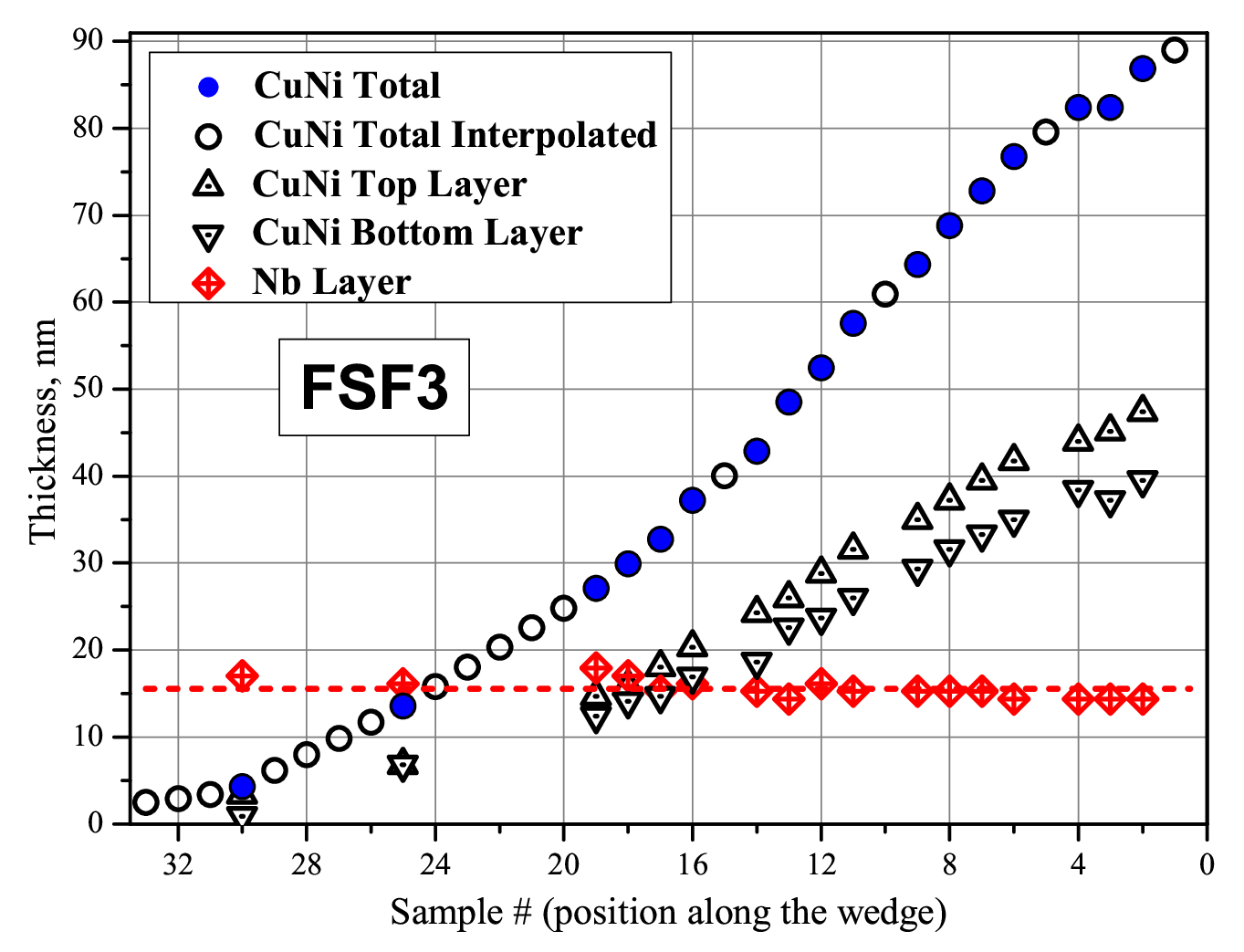
The RBS spectra fitting procedure is described in Ref. [47]. The results of the RBS evaluation are presented in Fig. 2. Depending on the sample, the graph shows almost linearly increasing thicknesses of both copper-nickel layers from about 1 to 48 nm. The niobium layer thickness is nearly constant of around 15.5 nm (dashed line in Fig. 2) with slight tendency to increase for largest sample numbers. The thicknesses of both CuNi alloy layers were found to be nearly the same only for intermediate range of the samples (approximately for Nr. 20). However, the deviation of the CuNi layers thicknesses over the mean value mainly did not exceed 10 %.
2.3 Critical fields measurements
The critical field measurements were performed in a 4He cryostat equipped with a superconducting solenoid providing magnetic fields up to T. The temperature was controlled in the range of K with an accuracy of about mK. Resistivity measurements were performed in Oxford Instruments 4He-3He Heliox insert, using the conventional four-probe method. In order to avoid thermoelectric voltages, alternating of the current polarity was performed during our measurements. The resistive transitions for the sample #26 are displayed in Fig. 3 for different values of the magnetic field. The critical temperatures assigned to the applied field, i.e. the upper critical magnetic field , were determined as midpoints of the resistive transitions . The estimated accuracy of the evaluation is within a few mK. The critical values of the magnetic field were measured for two field orientations – perpendicular and parallel to the sample plane, and respectively. Both the critical temperature values and the slope of the curves in the vicinity of are listed in Table 1.

| Sample number | 33 | 31 | 28 | 26 | 20 | 15 | 10 | 5 | 1 |
|---|---|---|---|---|---|---|---|---|---|
| 2.5 | 3.4 | 6.6 | 10.8 | 23.9 | 39.6 | 60.1 | 79.5 | 89.0 | |
| (K) | 6.73 | 6.7 | 5.25 | 2.40 | 2.69 | 2.86 | 2.98 | 3.00 | 3.35 |
| (T/K) | -0.522 | -0.469 | -0.477 | -0.236 | -0.216 | -0.221 | -0.217 | -0.217 | -0.216 |
Figure 4 displays the temperature dependencies for perpendicular (left panel) and parallel (right panel) critical magnetic fields for the FSF3 series with the niobium layer thickness value nm. One observes that both critical fields demonstrate a non-monotonous dependence on the ferromagnetic CuNi layer thickness. This observation requires an explanation which will be obtained by means of our theoretical analysis developed in the next section.


3 Theory
In this Section we elaborate a theoretical analysis of the superconducting phase transition in F1SF2 trilayers in the presence of an external magnetic field. A sketch of our trilayer is shown in Fig. 5.

Our treatment is based on the quasiclassical theory of superconductivity. As in the vast majority of experiments the electron elastic mean free path in both superconducting and ferromagnetic layers remain much smaller than the coherence length , and , respectively, where is the exchange energy, it would be appropriate to stick to the so-called dirty limit and apply the Usadel equations [31, 48]. In addition, we will make use of the fact that at temperatures sufficiently close to the critical one, , the superconducting order parameter is much smaller than temperature, . In this limit, one can linearize the Usadel equations for the anomalous quasiclassical Green function and obtain
| (1) |
where is the diffusion constant, is the vector potential, is the Matsubara frequency and is the exchange field in the ferromagnet. The exchange field and the superconducting order parameter differ from zero, respectively, in the ferromagnetic and superconducting layers only. For simplicity, in what follows, we will assume that the magnetization in each ferromagnetic layer is spatially uniform within this layer, and that mutual orientation of the two magnetizations is collinear, i.e. either parallel (P), or antiparallel (AP).
Equation (1) should be supplemented by appropriate boundary conditions matching the -functions at the S/F interfaces [49, 50]. In the vicinity of the critical temperature these boundary conditions read
| (2) |
where is the interface resistance per unit area, and are the Drude conductivities and anomalous Green functions at both sides of the corresponding S/F interface, respectively. Below we will consider two orientations of the external magnetic field: perpendicular and parallel to the S/F interfaces.
3.1 Perpendicular upper critical field
Let us first consider an F1SF2 structure subject to an external magnetic field perpendicular to the S/F interfaces. In order to account for a uniform magnetic field we can choose the gauge , where , are in-plane coordinates, and -axis is perpendicular to the layers’ plane. In this case we can use the following Ansatz for both the anomalous Green function and the order parameter [51]
| (3) | |||
| (4) |
where the function obeys the equation
| (5) |
and is the flux quantum. Then, Eq. (1) takes the form
| (6) |
Since the magnetic field enters only through the second term in Eq. (6), in order to obtain the critical field it suffices to restrict our analysis to the lowest Landau level, i.e. to set .
In the ferromagnetic regions the superconducting order parameter equals to zero identically, and Eq. (6) can be solved exactly. In the superconducting region it is necessary to obtain the solution of the equation
| (7) |
with the effective boundary conditions
| (8) | |||
| (9) |
where the parameters account for the influence of the top and the bottom ferromagnetic layers, respectively, on the superconducting layer. They read
| (10) | |||
| (11) |
where and denote the conductivities and the diffusion constants in the superconductor and in the two ferromagnetic layers with thicknesses , , and , respectively (see Fig. 5). Exchange fields of the ferromagnets are denoted by and . The interface resistances per unit area and refer to the S/F1- and S/F2-interface resistances.
Spatial dependence of the superconducting order parameter is fixed by the self-consistency equation
| (12) |
where is the BCS coupling constant, and defines the high frequency cutoff, which is typically of the order of corresponding Debye frequency. Introducing the superconducting critical temperature in the absence of both the external magnetic field and the ferromagnetic layers one can expel and from Eq. (12) and get
| (13) |
where ().
The critical magnetic field is determined by a highest value of at which the system of equations (7)-(9), (13) still has a non-trivial solution. In order to proceed further we will employ the fundamental solution method [52]. It is convenient to introduce the function which inside the superconductor () obeys the following equation
| (14) | |||
| (15) |
together with the corresponding boundary conditions at the SF interfaces
| (16) | |||
| (17) |
Equations (14)-(17) can be resolved analytically with the result
| (18) |
The solution of Eqs. (7)-(9) can now be expressed as a convolution of the function and the spatially dependent order parameter :
| (19) |
Combining Eqs. (13) and (19) we effectively reduce our problem to the integral equation for the superconducting order parameter which can be resolved in a straightforward way.
To proceed with numerical solution it is useful to discretize this integral equation employing the Fourier transformation
| (20) | |||
| (21) |
Then, the integral equation can be transformed into an infinite system of linear equations,
| (22) |
which can be reduced by a partial summation over the Matsubara frequencies to a form:
| (23) |
where is digamma function. The matrix elements describe the strength of the proximity effect in the superconducting layer. They are defined by the following expression,
| (24) |
3.2 Parallel upper critical field
Let us now turn to a configuration of the external magnetic field oriented parallel to the S/F interfaces. For a uniform magnetic field we choose the gauge and employ the following Ansatz for the anomalous Green function and the order parameter [30],
| (25) | |||
| (26) |
where is a free parameter which should be chosen in a way to maximize the critical magnetic field (or temperature). Then, the Usadel equation (1) reduces to
| (27) |
As before, we can effectively transform the above differential equation into an integral one:
| (28) |
where now
| (29) |
and denote two linearly independent solutions of the equation
| (30) |
The parameters and are defined by the following relations
| (31) | |||
| (32) |
and
| (33) |
is the Wronskian for the two solutions and . For simplicity we will assume that the orbital effects of the magnetic field in the ferromagnetic layers are small. Then, we can obtain parameters from Eqs. (10), (11) in which the external magnetic field should be set equal to zero . Combining Eq. (29) with the equations derived in Sec. 3A, we derive the upper critical field for the parallel orientation of the magnetic field.
On the basis of the analysis developed above the upper critical field was evaluated numerically for the both cases of perpendicular () and parallel () external magnetic fields. The corresponding results are presented in the next Section.
4 Comparison between the theory and experiment


Let us perform a detailed comparison between our experimental observations and theoretical results. By fitting our theoretical curves to the experimental data it becomes possible to estimate the parameters of our F1SF2 structures which could not be measured directly. Such fits for the perpendicular critical magnetic field measured in different F1SF2 samples are displayed in the left panel of Fig. 4 by solid lines along with the experimental data points denoted by symbols. The thickness of the S-layer remains the same for all samples in a series. The same set of parameters was employed to fit all the experimental data presented in Fig. 4. These parameters are:
| (34) | |||
| (35) | |||
| (36) |
Unfortunately, our fitting procedure does not allow to unambiguously determine the interface resistances . From Eq. (10) we observe that under the condition
| (37) |
the critical temperature remains almost insensitive to the values . Making use of the fact that the best fit of our data is obtained for fully transparent interfaces and employing the parameter values (34)- (36) we arrive at an estimate
| (38) |
Our theoretical results for the parallel critical magnetic field (solid lines) are presented in the right panel of Fig. 4 for the same values of fitting parameters (34)-(36).
In both cases of perpendicular and parallel magnetic field configurations we observe a reasonably good agreement between the theory and the experiment, in particular, having in mind that single set of the fitting parameters was used for all our samples. Further improvement of the quality of our fits can be achieved by a small adjustment of these parameters individually for each sample. We note that one can indeed expect such parameters as exchange field , conductivity and diffusion constant to be slightly different for the ferromagnetic layers, since these parameters may depend, e.g., on the layer thickness and different growth conditions for the bottom and top CuNi layers. There exists also a number of other physical reasons which might be responsible for a small mismatch between the theoretical curves and the corresponding experimental data in Fig. 4. One of such reasons is that the standard weak-coupling BCS theory of superconductivity employed here can describe the properties of niobium samples only approximately [53]: strong coupling corrections to this theory may easily reach in this case. This observation alone appears to be sufficient to account for the remaining discrepancies between the theory and experiment. In addition, the quasiclassical Usadel equation formalism employed here yields quantitatively correct results only provided the condition is fulfilled in ferromagnetic metals. It is not completely clear if this condition is well satisfied in our samples, which are in the intermediate regime between strong and weak ferromagnets. Bearing all the above in mind we conclude that our theory sufficiently well describes the experimental data for the critical magnetic field in all our samples.
To complete our analysis, in Fig. 6 we display both our theoretical results (solid lines) and the experimental data (symbols) for the superconducting critical temperature as a function of the total thickness of the ferromagnetic layers at different magnitudes of the applied magnetic field. A good agreement between the theory and experiment is observed for all samples. At low magnetic field exhibits nonmonotonous oscillatory dependence which becomes reentrant at high enough magnetic fields (the curves from top to bottom in Fig. 6, see also Ref. [54]).
In conclusion, we have experimentally and theoretically analyzed the upper critical field in F1SF2 trilayers in both perpendicular and parallel geometries. The series of samples with variable thicknesses of F-layers were prepared in a single run utilizing the original wedge deposition and moving magnetron techniques. The sample series exhibit an oscillatory behavior in absence of an external magnetic field, so several characteristic points in this dependence were chosen for the critical fields measurements. Perpendicular and parallel critical fields were measured in the same samples in the temperature range K and for magnetic fields up to 9 Tesla. A transition from the oscillatory to the reentrant behavior of , driven by the external magnetic field, was observed for the first time. Temperature dependence of the critical magnetic field was derived from the quasiclassical Usadel equations for arbitrary values of the system parameters, such as superconducting transition temperature of the stand-alone superconducting layer , superconducting coherence length , exchange splitting energies in the F-layers, conductivities of the ferromagnetic and superconducting layers , conduction diffusion coefficients in the F and S layers, and the interface resistances for the S/F1- and S/F2 interfaces, respectively. A fairly good agreement between our theoretical predictions and the sets of the experimental data on for different magnetic layers thickness, as well as at different magnitudes of the magnetic field, has been achieved for a single set of fit parameters. The transition from the oscillatory to the reentrant behavior in magnetic field has been successfully described by the theory. On one hand, this observation demonstrates consistency of the FFLO physics (described within the Usadel equation formalism) with the experimental findings obtained in our particular Cu41Ni59/Nb/Cu41Ni59 trilayer spin-valve cores. On the other hand, the theory allows to include more experimental data to rectify conditions for obtaining sizable spin-valve effect in superconductor-ferromagnet heterostructures.
Aknowledgements
We would like to thank V. V. Ryazanov, M. Yu. Kupriyanov and A. I. Buzdin for useful discussions as well as M. Schreck and S. Gsell for help with RBS measurements. The work is supported by A. von Humboldt Foundation within the frame of the Institutspartnerschaften Project and in part by the DFG grant No. GZ: HO 955/6-2.
References
References
- [1] Werthamer R, Helfand E and Hoenberg P C 1966 Phys. Rev. B 147 295
- [2] Zwicknagl G E and Wilkins J W 1984 Phys. Rev. Lett. 53 1276
- [3] Larkin A I and Y N Ovchinnikov 1971 Zh. Eksp. Teor. Fiz. 61 1221 [1971 Sov. Phys. JETP 34 651]
- [4] Lee I J, Naughton M J, Danner G M and Chaikin P M 1997 Phys. Rev. Lett. 78 3555
- [5] Drechsler S -L, Rosner H, Shulga S V , Eschrig H , Freudenberger J, Fuchs G, Nenkov K, Müller K -H, Lipp D, Gladun A, Kreyssig A, Koepernik K, Gegenwart P and Cichorek T 2000 Physica C 341-348 749
- [6] B.Y. Jin and J.B. Ketterson 1989 Adv. Phys. 38 189
- [7] Buzdin A I 2005 Rev. Mod. Phys. 77 935
- [8] Bergeret F S, Volkov A F and Efetov K B 2005 Rev. Mod. Phys. 77 1321
- [9] Lyuksyutov I F and Pokrovsky V L 2005 Adv. Phys. 54 67
- [10] Golubov A A, Kupriyanov M Yu and Il’ichev E 2004 Rev. Mod. Phys. 76 411
- [11] Khabipov M I , Balashov D V, Maibaum F, Zorin A B, Oboznov V A, Bol’ginov V V, Rossolenko A N and Ryazanov V V 2010 Supercond. Sci. Technol. 23 045032
- [12] Feofanov A K, Oboznov V A, Bol’ginov V V, Lisenfeld J, Poletto S, Ryazanov V V, Rossolenko A N, Khabipov M, Balashov D, Zorin A B, Dmitriev P N, Koshelets V P and Ustinov A V 2010 Nature Physics Letters 6 593
- [13] Oh S, Youm D and Beasley M R 1997 Appl. Phys. Lett. 71 2376
- [14] Tagirov L R 1999 Phys. Rev. Lett. 83 2058
- [15] Buzdin A I, Vedyayev A V and Ryzhanova N V 1999 Europhys. Lett. 48 686
- [16] Gu J Y, You C Y, Jiang J S, Pearson J, Bazaliy Ya B and Bader S D 2002 Phys. Rev. Lett. 89 267001
- [17] Fominov Ya V, Golubov A A, Karminskaya T Yu, Kupriyanov M Yu, Deminov R G and Tagirov L R 2010 Pis’ma v ZhETF 91 329 [2010 JETP Lett. 91 308]
- [18] Karminskaya T Yu and Kupriyanov M Yu 2007 Pis’ma v ZhETF 86 65 [2007 JETP Lett. 86 61]
- [19] Houzet M and Buzdin A I 2007 Phys. Rev. B 76 060504(R)
- [20] Karminskaya T Yu and Kupriyanov M Yu and Golubov A A 2008 Pis’ma v ZhETF 87 657 [2008 JETP Lett. 87 570]
- [21] Luo Y and Samwer K, 2010 Europhys Lett. 91 37003
- [22] Leksin P V, Garif’yanov N N, Garifullin I A, Schumann J, Vinzelberg H, Kataev V E, Klingeler R, Schmidt O G and Büchner B 2010 Appl. Phys. Lett. 97 102505
- [23] Leksin P V, Garif’yanov N N, Garifullin I A, Schumann J, Vinzelberg H, Kataev V E, Schmidt O G and Büchner B 2011 Phys. Rev. Lett. 106 067005
- [24] Leksin P V, Garif’yanov N N, Garifullin I A, Fominov Ya V, Schumann J, Krupskaya Y, Kataev V E, Schmidt O G and Büchner B 2012 Phys. Rev. Lett. 109 057005
- [25] Zdravkov V I, Kehrle J, Obermeier G, Lenk D, Krug von Nidda H -A, Müller C, Kupriyanov M Yu, Sidorenko A S, Horn S, Tidecks R. and Tagirov L R 2013 Phys. Rev. B 87 144507
- [26] Bol’ginov V V, Stolyarov V S, Sobanin D S, Karpovich A L and Ryazanov V V 2012 Pis’ma v ZhETF 95 408 [2010 JETP Lett. 95 366]
- [27] Larkin T I, Bol’ginov V V, Stolyarov V S, Ryazanov V V, Sobanin D S, Vernick I V, Tolpygo S K and Mukhanov O A 2012 Appl. Phys. Lett. 100 222601
- [28] Radović Z, Dobrosavljević-Grujić L, Buzdin A I and Clem J R 1988 Phys. Rev. B 38 2388
- [29] Kuboya K and Takanaka K 1998 Phys. Rev. B 57 6022
- [30] Krunavakarn B and Yoksan S 2006 Physica C 440 25
- [31] Usadel K D 1970 Phys. Rev. Lett. 25 507
- [32] Fulde P and Ferrell R 1964 Phys. Rev. 135 A550
- [33] Larkin A I and Ovchinnikov Yu N 1964 Zh. Eksp. Teor. Fiz. 47 1136 [1965 Sov. Phys. JETP 20 762]
- [34] Chien C L and Daniel H Reich 1999 J. Magn. Magn. Mater. 200 83
- [35] Verbanck G, Potter C D, Schad R, Beilen P, Moshchalkov V V, and Bruynseraede 1994 Physica C 235-240 3295
- [36] Koorevaar P, Coehoorn R, Aarts J 1995 Physica C 248 61
- [37] Mattson J E, Potter C D, Conover M J, Sowers C H and Bader S D 1997 Phys. Rev. B 55 70
- [38] Verbanck G, Potter C D, Metlushko V, Schad R, Moshchalkov V V, and Bruynseraede 1998 Phys. Rev. B 57 6029
- [39] Prischepa S L, Cirillo C, Bell C, Kushnir V N, Aarts J, Attanasio C, and Kupriyanov M Yu 2008 Pis’ma v ZhETF 88 375 [2008 JETP Lett. 88 431]
- [40] Armenio A A, Cirillo C, Iannone G, Prischepa S L and Attanasio C 2007 Phys. Rev. B 76 024515
- [41] Huang S Y, Liang J.-J, Tsai T C, Lin L K, Lin M S, Hsu S Y and Lee S F 2008 Journ. Appl. Phys. 103 07C704
- [42] Cirillo C, Bell L C, Iannone G, Prischepa S L, Aarts J and Attanasio C 2009 Phys. Rev. B 80 094510
- [43] Zdravkov V I, Kehrle J, Obermeier G, Gsell S, Schreck M, Müller C, Krug von Nidda H -A, Lindner J, Moosburger-Will J, Nold E, Morari R, Ryazanov V V, Sidorenko A S, Horn S, Tidecks R and Tagirov L R 2010 Phys. Rev. B 82 054517
- [44] Zdravkov V, Sidorenko A, Obermeier G, Gsell S, Schreck M, Müller C, Horn S, Tidecks R and Tagirov L R 2006 Phys. Rev. Lett. 97 057004
- [45] Sidorenko A S, Zdravkov V I, Kehrle J, Morari R, Antropov E, Obermeier G, Gsell S, Schreck M, Müller C, Ryazanov V V, Horn S, Tidecks R and Tagirov L R 2009 in Nanoscale Phenomena—Fundamentals and Applications (NanoScience and Technology Series vol 18) ed Hahn H, Sidorenko A and Tiginyanu I (Berlin: Springer-Verlag) p 3-11
- [46] Zdravkov V I, Kehrle J, Obermeier G, Ullrich A, Gsell S, Lenk D, Müller C, Morari R, Sidorenko A S, Ryazanov V V, Tagirov L R, Tidecks R and Horn S 2011 Supercond. Sci. Technol. 24 095004
- [47] Kehrle J, Zdravkov V I, Obermeier G, Garcia-Garcia J, Ullrich A, C. Müller, Morari R, Sidorenko A S, Horn S, Tidecks R and Tagirov L R 2012 Ann. Phys. (Berlin) 525 37
- [48] Belzig W, Wilhelm F K, Bruder C, Schön G and Zaikin A D 1999 Superlatt. Microstruct. 25 1251
- [49] Kuprianov M Yu and Lukichev V F 1988 Zh. Eksp. Teor. Fiz. 94 139 [1988 Sov. Phys. JETP 67 1163]
- [50] Tagirov L R and Garcia N 2007 Superlatt. Microstruct. 41 152
- [51] Radović Z, Ledvij M and Dobrosavljević-Grujić L 1991 Solid State Commun. 80 43
- [52] Fominov Ya V, Chtchelkatchev N M and Golubov A A 2002 Phys. Rev. B 66 014507
- [53] Carbotte J P 1990 Rev. Mod. Phys. 62 1027
- [54] Avdeev M, Khusainov M, Proshin Yu, and Tsarevskii S 2010 Supercond. Sci. Technol. 23 105005