Wireless Information and Power Transfer: A Dynamic Power Splitting Approach
Abstract
Energy harvesting is a promising solution to prolong the operation time of energy-constrained wireless networks. In particular, scavenging energy from ambient radio signals, namely wireless energy harvesting (WEH), has recently drawn significant attention. In this paper, we consider a point-to-point wireless link over the flat-fading channel, where the receiver has no fixed power supplies and thus needs to replenish energy via WEH from the signals sent by the transmitter. We first consider a SISO (single-input single-output) system where the single-antenna receiver cannot decode information and harvest energy independently from the same signal received. Under this practical constraint, we propose a dynamic power splitting (DPS) scheme, where the received signal is split into two streams with adjustable power levels for information decoding and energy harvesting separately based on the instantaneous channel condition that is assumed to be known at the receiver. We derive the optimal power splitting rule at the receiver to achieve various trade-offs between the maximum ergodic capacity for information transfer and the maximum average harvested energy for power transfer, which are characterized by the boundary of a so-called “rate-energy” region. Moreover, for the case when the channel state information is also known at the transmitter, we investigate the joint optimization of transmitter power control and receiver power splitting. The achievable rate-energy (R-E) region by the proposed DPS scheme is compared against that by the existing time switching scheme as well as a performance upper bound by ignoring the practical receiver constraint. Finally, we extend the result for DPS to the SIMO (single-input multiple-output) system where the receiver is equipped with multiple antennas. In particular, we investigate a low-complexity power splitting scheme, namely antenna switching, which can be practically implemented to achieve the near-optimal rate-energy trade-offs as compared to the optimal DPS.
Index Terms:
Energy harvesting, wireless power transfer, power control, fading channel, ergodic capacity, multiple-antenna system, power splitting, time switching, antenna switching.I Introduction
Recently, energy harvesting has become a prominent solution to prolong the lifetime of energy-constrained wireless networks, such as sensor networks. Compared with conventional energy supplies such as batteries that have fixed operation time, energy harvesting from the environment potentially provides an unlimited energy supply for wireless networks. Besides other commonly used energy sources such as solar and wind, radio frequency (RF) signal holds a promising future for wireless energy harvesting (WEH) since it can also be used to provide wireless information transmission at the same time, which has motivated an upsurge of research interest on RF-based wireless information and power transfer recently [1]-[5]. Prior works [1], [2] have studied the fundamental performance limits of wireless systems with simultaneous information and power transfer, where the receiver is ideally assumed to be able to decode the information and harvest the energy independently from the same received signal. However, this assumption implies that the received signal used for harvesting energy can be reused for decoding information without any loss, which is not realizable yet due to practical circuit limitations. Consequently, in [3] the authors proposed two practical receiver designs, namely “time switching”, where the receiver switches between decoding information and harvesting energy at any time, and “power splitting”, where the receiver splits the signal into two streams of different power for decoding information and harvesting energy separately, to enable WEH with simultaneous information transmission.
In this paper, we further investigate the power splitting scheme in [3] for a point-to-point single-antenna flat-fading channel, where the receiver is able to dynamically adjust the split power ratio for information decoding and energy harvesting based on the channel state information (CSI) that is assumed to be known at the receiver, a scheme so-called “dynamic power splitting (DPS)” as shown in Fig. 1. We assume that the transmitter has a constant power supply, whereas the receiver has no fixed power supplies and thus needs to harvest energy from the received signal sent by the transmitter. For the ease of hardware implementation, we consider the case where the information decoding circuit and energy harvesting circuit are separately designed (as opposed to an integrated design in [4]). As a result, the receiver needs to determine the amount of received signal power that is split to the information receiver versus that to the energy receiver based on the instantaneous channel power. We derive the optimal power splitting rule at the receiver to achieve various tradeoffs between the maximum ergodic capacity for information transmission versus the maximum average harvested energy for power transmission, which are characterized by the boundary of a so-called “rate-energy (R-E)” region. Moreover, for the case of CSI also known at the transmitter (CSIT), we examine the joint optimization of transmitter power control and receiver power splitting, and show the achievable R-E gains over the case without CSIT.
Furthermore, we extend the DPS scheme for the single-input single-output (SISO) system to the single-input multiple-output (SIMO) system, where the receiver is equipped with multiple antennas. After deriving the optimal DPS rule for the SIMO system which in general requires independent power splitters that are connected to different receiving antennas, we further investigate a low-complexity power splitting scheme so-called “antenna switching” proposed in [3], whereby the total number of receiving antennas is divided into two subsets, one for decoding information and the other for harvesting energy. It is noted that for the SISO fading channel case, antenna switching reduces to time switching, which has been studied in our previous work [5]. In [5], the optimal time switching rule based on the receiver CSI and its corresponding transmitter power control policy (in the case of CSI known at the transmitter) were derived to achieve various trade-offs between wireless information and energy transfer. It was shown that for time switching, the optimal policy is threshold based, i.e., the receiver decodes information when the fading channel gain is below a certain threshold, and harvests energy otherwise. It is worth noting that although theoretically time switching can be regarded as a special form of power splitting with only on-off power allocation at each receiving antenna, they are implemented by different hardware circuits (time switcher versus power splitter) in practice.
The main results of this paper are summarized as follows:
- •
For the SISO case, we show that to achieve the optimal R-E trade-offs in both the cases without or with CSIT by DPS, a fixed amount of the received signal power should be allocated to the information receiver, with the remaining power allocated to the energy receiver when the fading channel gain is above a given threshold. However, when the fading channel gain is below this threshold, all the received power should be allocated to the information receiver. Compared with our previous result for the time switching receiver in [5] where only the energy harvesting receiver can benefit from “good” fading channels above the threshold, the DPS scheme utilizes the “good” fading states for both information decoding and energy harvesting. As a result, we show by simulations that DPS can achieve substantial R-E performance gains over dynamic time switching in the SISO fading channel. Moreover, we derive the R-E region for the ideal case when the receiver can decode information and harvest energy from the same received signal independently without any rate or energy loss, which provides a theoretical performance upper bound for the DPS scheme.
- •
For the SIMO case where the receiver is equipped with multiple antennas, we extend the result for DPS as follows. First, we show that a uniform power splitting (UPS) scheme where all the receiving antennas are assigned with the same power splitting ratio is optimal. We derive the optimal UPS rule and/or transmitter power control (in the case with CSIT) based on the result for the SISO system by treating all the receiving antennas as one virtual antenna with an equivalent channel sum-power. Second, to ease the hardware implementation of UPS, we investigate the optimal antenna switching rule to maximize the achievable R-E trade-offs. An exhaustive search algorithm is presented first, and then a new low-complexity antenna selection algorithm is proposed, which is shown to perform closer to the optimal UPS as the number of receiving antennas increases. Moreover, it is shown that with the optimal antenna selection, even with two receiving antennas, the R-E performance of antenna switching is already very close to that with the optimal UPS. This demonstrates the usefulness of antenna switching as a practically appealing low-complexity implementation for power splitting.
The rest of this paper is organized as follows. Section II presents the system model and illustrates the encoding and decoding schemes for wireless information transfer with opportunistic energy harvesting by DPS. Section III defines the R-E region achievable by DPS and formulates the problems to characterize its boundaries without or with CSIT. Sections IV presents the optimal DPS rule at the receiver and/or power control policy at the transmitter (in the case of CSIT) to achieve various R-E trade-offs in the SISO fading channel. Section V extends the result to the SIMO fading channel and investigates the practical scheme of antenna switching. Finally, Section VI concludes the paper.
II System Model

As shown in Fig. 1, we first consider a wireless SISO link consisting of one pair of single-antenna transmitter (Tx) and single-antenna receiver (Rx) over the flat-fading channel. The case of single-antenna Tx and multi-antenna Rx or SIMO system will be addressed later in Section V. For convenience, we assume that the channel from Tx to Rx follows a block-fading model [6], [7]. The equivalent complex baseband channel from Tx to Rx in one particular fading state is denoted by , where denotes the fading state, and the channel power gain at fading state is denoted by . It is assumed that the random variable (RV) has a continuous probability density function (PDF) denoted by . At any fading state , is assumed to be perfectly known at Rx, but may or may not be known at Tx.
We consider time-slotted transmissions at Tx and the DPS scheme at Rx. As shown in Fig. 1, at Rx, the RF-band signal is corrupted by an additive noise introduced by the receiver antenna, which is assumed to be a circularly symmetric complex Gaussian (CSCG) RV with zero mean and variance , denoted by , in its baseband equivalent. The RF-band signal is then fed into a power splitter [8], [9], where the signal plus the antenna noise is split to the information receiver and energy receiver [10] separately. For each fading state , the portion of signal power split to information decoding (ID) is denoted by with , and that to energy harvesting (EH) as , where in general can be adjusted over different fading states. The ID circuit introduces an additional baseband noise to the signal split to the information receiver, which is assumed to be a CSCG RV with zero mean and variance , and independent of the antenna noise . As a result, the equivalent noise power for ID is at fading state . On the other hand, in addition to the split signal energy, the energy receiver can harvest amount of energy (normalized by the slot duration) due to the antenna noise . However, in practice, has a negligible influence on both the ID and EH since is usually much smaller than the noise power introduced by the information receiver, , and thus even lower than the average power of the received signal. Thus, in the rest of this paper, we assume for simplicity.
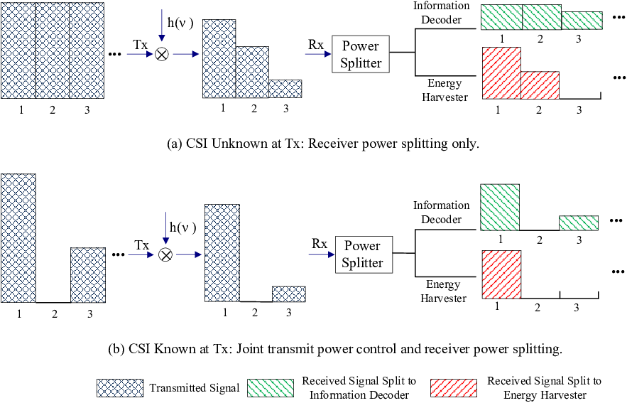
For the DPS scheme, we describe the enabling encoding and decoding strategies for the following two cases. Case I: is unknown at Tx for all the fading states of , referred to as CSI Unknown at Tx; and Case II: is perfectly known at Tx for each fading state , referred to as CSI Known at Tx (CSIT).
First, consider the case of CSI Unknown at Tx, which is depicted in Fig. 2(a). In this case, Tx sends information continuously with constant power for all the fading states due to the lack of CSIT [11]. At each fading state , Rx determines the optimal power ratio allocated to the information decoder and the energy harvester , based on . For example, as shown in Fig. 2(a), in time slot 3, all the received power is allocated to the information decoder (i.e., ), while in time slots 1 and 2, the received power is split to both the information decoder and energy harvester (i.e., ).
Next, consider the case of CSIT as shown in Fig. 2(b). In this case, Tx is able to schedule transmissions for information and energy transfer to Rx based on . As will be shown later in Section IV-B, the optimal power splitting rule in this case always has provided that the transmitted power is non-zero. As a result, without loss of generality, we can assume that at any fading state , Tx either transmits information signal or does not transmit at all (to save power). For example, in Fig. 2(b), Tx transmits information signal in time slots 1 and 3, and transmits no signal in time slot 2. Accordingly, Rx splits the received signal to the information decoder and the energy receiver (i.e., ) in slot 1, but allocates all the received power to the information receiver in time slot 3 (i.e., ). Moreover, Tx can implement power control based on the instantaneous CSI to further improve the information and energy transmission efficiency. Let denote the transmit power of Tx at fading state . In this paper, we consider two types of power constraints on , namely average power constraint (APC) and peak power constraint (PPC). The APC limits the average transmit power of Tx over all the fading states, i.e., , where denotes the expectation over . In contrast, the PPC constrains the instantaneous transmit power of Tx at each of the fading states, i.e., , . Without loss of generality, we assume . For convenience, we define the set of feasible power allocation as
| (1) |
It is worth noting that for the case without CSIT, a fixed transmit power is assumed with , , such that both the APC and PPC are satisfied.
III Rate and Energy Trade-off in the SISO Fading Channel
In this paper, we consider the ergodic capacity as a relevant performance metric for information transfer. For the DPS scheme, given and , the instantaneous mutual information (IMI) for the Tx-Rx link at fading state is expressed as
| (2) |
As a result, the ergodic capacity can be expressed as [11]
| (3) |
For information transfer, if CSIT is not available, the ergodic capacity can be achieved by a single Gaussian codebook with constant transmit power over all different fading states [12]; however, with CSIT, the ergodic capacity can be further maximized by the “water-filling (WF)” based power allocation subject to the peak power constraint [13], [14].
On the other hand, for wireless energy transfer, the harvested energy (normalized by the slot duration) at each fading state can be expressed as , where is a constant that accounts for the loss in the energy transducer for converting the harvested energy to electrical energy to be stored; for convenience, it is assumed that in the rest of this paper unless stated otherwise. We thus have
| (4) |
The average energy that is harvested at Rx is then given by
| (5) |
Evidently, there exist trade-offs in assigning the power splitting ratio and/or transmit power (in the case of CSIT) to balance between maximizing the ergodic capacity for information transfer versus maximizing the average harvested energy for power transfer. To characterize such trade-offs, we adopt the so-called Rate-Energy (R-E) region (defined below) as introduced in [3], [5], which consists of all the achievable ergodic capacity and average harvested energy pairs given a power constraint in (1). Specifically, in the case without (w/o) CSIT, the R-E region is defined as
| (6) |
while in the case with CSIT, the R-E region is defined as
| (7) |

Fig. 3 shows some examples of the R-E region without versus with CSIT by the DPS scheme (see Section IV for the details of computing these regions). It is assumed that the average transmit power constraint is watt(W) or dBm, and the peak power constraint is W or dBm. The average operating distance between Tx and Rx is assumed to be meters, which results in an average of dB signal power attenuation at a carrier frequency assumed as MHz. With this distance, the line-of-sight (LOS) signal plays the dominant role, and thus Rician fading is used to model the channel. Specifically, at each fading state , the complex channel can be modeled as , where is the LOS deterministic component with dB (to be consistent with the average path loss), denotes the Rayleigh fading component, and is the Rician factor specifying the power ratio between the LOS and fading components in . Here we set . The bandwidth of the transmitted signal is assumed to be MHz, and the information receiver noise is assumed to be white Gaussian with power spectral density dBm/Hz or dBm over the entire bandwidth of MHz. Moreover, the energy conversion efficiency for the energy harvester is assumed to be . For comparison, we also show the R-E regions by a special form of DPS known as time switching [5] under the same channel setup with or without CSIT. Furthermore, the R-E regions obtained by assuming that the receiver can ideally decode information and harvest energy from the same received signal without any rate/power loss [2] are added as a performance upper bound for DPS and time switching. It is observed that CSIT helps improve the achievable R-E pairs at the receiver for both DPS and time switching schemes. Moreover, as compared to time switching, DPS achieves substantially improved R-E trade-offs towards the performance upper bound. For example, when of the maximum harvested energy is achieved, the ergodic capacity is increased by for the case with CSIT and for the case without CSIT, by comparing DPS versus time switching. It is also observed that when the average harvested power is smaller than uW, DPS for the case without CSIT even outperforms time switching for the case with CSIT.
In Fig. 3, there are two boundary points shown in each R-E region, which are denoted by , for the case without CSIT, and , for the case with CSIT. For example, for the R-E trade-offs in the case without CSIT, we have
| (8) | ||||
| (9) |
Note that is achieved when , , and thus the resulting ergodic capacity is zero, while is achieved when , , and thus the resulting harvested energy is zero. The above holds for both time switching and power splitting receivers. Similarly, and in the case with CSIT can be obtained, while for brevity, their expressions are omitted here. It is worth noting that in general due to the WF-based power control. However, with high signal-to-noise ratio (SNR), the rate gain by transmitter power control is negligibly small. As a result, in Fig. 3 and are observed to be very close to each other.
Since the optimal trade-offs between the ergodic capacity and the average harvested energy are characterized by the boundary of the R-E region, it is important to characterize all the boundary pairs for DPS in both the cases without and with CSIT. Similarly as for the case of time switching in [5], to characterize the Parato boundary of the R-E region for DPS, we need to solve the following two optimization problems.
where is a target average harvested energy required to maintain the receiver’s operation. By solving Problem (P1) for all and Problem (P2) for all , we can characterize the entire boundary of the R-E region for the case without CSIT (defined in (6)) and with CSIT (defined in (7)), respectively.
Problem (P1) is a convex optimization problem in terms of ’s, whereas Problem (P2) is non-convex in general since both the objective and harvested energy constraint are non-concave functions over and . However, it can be verified that the Lagrangian duality method can still be applied to solve Problem (P2) globally optimally, i.e., (P2) has strong duality or zero duality gap [16].
Lemma III.1
Let and denote the optimal solutions to Problem (P2) given the average harvested energy constraint and average transmit power constraint pairs and , respectively. Then for any , there always exists a feasible solution such that
where with , and .
Proof:
Please refer to Appendix -A. ∎
Let denote the optimal value of (P2) given the average harvested energy constraint and the average power constraint . Lemma III.1 implies that the “time-sharing” condition in [15] holds for (P2), and thus is concave in , which then yields the zero duality gap of Problem (P2) according to the convex analysis in [16]. Therefore, in the next section, we will apply the Lagrange duality method to solve both (P1) and (P2).
IV Optimal Policy for the SISO Fading Channel
In this section, we study the optimal power splitting policy at Rx and/or power control policy at Tx to achieve various optimal rate and energy trade-offs in the SISO fading channel for both the cases without and with CSIT by solving Problems (P1) and (P2), respectively.
IV-A The Case Without CSIT
First, we consider Problem (P1) for the unknown CSIT case to determine the optimal power splitting rule at Rx with constant transmit power at Tx. The Lagrangian of Problem (P1) is expressed as
| (10) |
where is the dual variable associated with the harvested energy constraint . Then, the Lagrange dual function of Problem (P1) is given by
| (11) |
The maximization problem (11) can be decoupled into parallel subproblems all having the same structure and each for one fading state. For a particular fading state , the associated subproblem is expressed as
| (12) |
where
| (13) |
Note that in the above we have dropped the index for the fading state for brevity.
With a given , Problem (11) can be efficiently solved by solving Problem (12) for different fading states of . Problem (P1) is then solved by iteratively solving (11) with fixed , and updating via a simple bisection method until the harvested energy constraint is met with equality [16]. Let denote the optimal dual solution that has a one-to-one correspondence to in Problem (P1). Then, we have the following proposition.
Proposition IV.1
The optimal solution to Problem (P1) is given by
Proof:
Please refer to Appendix -B. ∎
It can be inferred from Proposition IV.1 that the power allocated to information decoding is a constant for all the fading states with since . Thus, must hold in (IV.1). As a result, the achievable rate is a constant equal to for such fading states. On the other hand, if , all the received power is allocated to the information receiver. The above result is explained as follows. Suppose that if an amount of received power is allocated to information receiver, we gain in the achievable rate, but lose in the harvested energy. Since the utility for our optimization problem given in (13) at each fading state is the difference between the gain in the achievable rate and the loss in the harvested energy, the maximum utility is achieved when , which is a constant regardless of the fading state. Therefore, if the received power , i.e., , then the received power allocated to the information receiver should be a constant , and the remaining received power, i.e., , is allocated to the energy receiver. Otherwise, if the received power is less than , it should be totally allocated to the information receiver.
In the following, we compare the above optimal receiver power splitting rule to the optimal time switching rule proposed in [5] for the achievable R-E trade-offs in the case without CSIT. For convenience, let and denote the optimal dual solutions to Problem (P1) with DPS and its modified problem (by changing the constraint in (P1) to , ) with time switching, respectively, for the same given . Moreover, similarly as in [5], we define the time switching indicator function as follows:
We then have the following observations in order:
- •
When the fading state is “poor”, i.e., for time switching or for power splitting, where is the unique solution to the following equation given in [5]: , the optimal receiver strategy is to allocate all the received power to the information receiver for both cases of time switching and power splitting, i.e., . In other words, the power allocated to information receiver is , and that to energy receiver is .
- •
When the fading state is “good”, i.e., for time switching or for power splitting, all the received power is allocated to energy harvester for time switching, i.e., , while for power splitting, a constant power is allocated to the information receiver, with the remaining power allocated to the energy receiver.
To summarize, the main difference between the optimal time switching and power splitting polices in the case without CSIT lies in the above “good” fading states. Specifically, both information decoding and energy harvesting can benefit from such good fading states if power splitting is used, while only energy harvesting benefits if time switching is used. An illustration of the above difference in the received power allocation for power splitting versus time switching is given in Fig. 4.

IV-B The Case With CSIT
For the case with CSIT, in addition to the receiver’s DPS, the transmitter can implement power control to further improve the R-E trade-off. To jointly optimize the values of and , , we need to solve Problem (P2), shown as follows.
Let and denote the nonnegative dual variables corresponding to the average harvested energy constraint and average transmit power constraint in Problem (P2), respectively. Similarly as for Problem (P1), Problem (P2) can be decoupled into parallel subproblems each for one particular fading state and expressed as (by ignoring the fading index )
| (18) |
where
| (19) |
After solving Problem (18) with given and for all the fading states, we can update via the ellipsoid method [16]. It can be shown that the sub-gradient for updating is , where and denote the harvested energy and transmit power at fading state , respectively, obtained by solving Problem (18) for a given pair of and . Let and denote the optimal dual solutions to Problem (P2) for a given set of , and . Similarly as for Proposition IV.1, it can be shown that when , it must hold that . We then have the following proposition.
Proposition IV.2
By defining , the optimal solution to Problem (P2) is given by
If ,
if ,
Proof:
Please refer to Appendix -C. ∎
It is worth noting that similar to the case without CSIT, from Proposition IV.2 it follows that in the case with CSIT, if , a constant received power is allocated to the information receiver, while the remaining received power is allocated to the energy receiver; otherwise, if , all the received power is allocated to the information receiver.
Next, we compare the optimal power splitting and time switching for the achievable R-E trade-offs in the case with CSIT. For convenience, let and denote the optimal dual solutions to Problem (P2) with DPS and its modified form (by changing the constraint in (P2) as , ) with time switching, respectively. We then obtain the following observations:
- •
When the fading state is “poor”, i.e., for time switching or for power splitting, the optimal strategy is to switch off the transmission to save transmit power in both schemes.
- •
For moderate fading states with for time switching or for power splitting, where is the largest root of the following equation given in [5]: , the optimal strategy is to transmit information with water-filling power allocation at Tx (with the maximum transmit power capped by ) and allocate all the received power to information receiver in both schemes.
- •
When the fading state is “good”, i.e., for time switching or for power splitting, the optimal strategy of the transmitter is to transmit at peak power in both schemes. However, at the receiver, all the received power is allocated to the energy receiver for time switching, i.e., , while for power splitting, only a constant amount of the received power is allocated to information receiver with the remaining power allocated to the energy receiver.
To summarize, similar to the case without CSIT, the main difference between the optimal resource allocation polices between power splitting and time switching for the case with CSIT lies in the above “good” fading states. Specifically, both information decoding and energy harvesting can benefit from good fading states if power splitting is used, while only energy harvesting benefits if time switching is used. An illustration of the above transmitter power control and receiver power allocation policies for power splitting versus time switching is given in Fig. 5.


IV-C Performance Upper Bound
In this subsection, we derive a R-E region upper bound for DPS (as well as other practical receiver designs) by considering an ideal receiver that can simultaneously decode information and harvest energy from the same received signal without any information/energy loss. This is equivalent to setting in (2) and in (4) at the same time. In this case, the information rate and harvested energy at each fading state can be respectively expressed as
| (27) | ||||
| (28) |
For the case without CSIT, there is no trade-off between information and energy transfer from the above since , . As a result, as shown in Fig. 3, the R-E region upper bound for the case without CSIT is simply a box. On the other hand, in the case with CSIT, a trade-off between and given in (27) and (28) due to the power allocation policy , which has been similarly studied in [2] for the frequency-selective AWGN channel with simultaneous information and power transfer. By solving Problem (P2) for all feasible ’s, with and replaced by (27) and (28), respectively, the R-E region upper bound in the case of CSIT can be obtained. Let and denote the optimal dual solutions associated with the harvested energy constraint and average power constraint , respectively. By following the similar proof of Proposition IV.2, we can obtain the optimal power allocation for achieving the R-E region upper bound in the case with CSIT in the following proposition.
V Extension and Application: Dynamic Power Splitting for the SIMO Fading Channel
In this section, we extend the result for DPS to the SIMO fading channel, i.e., when the receiver is equipped with multiple antennas, and furthermore study a low-complexity implementation of power splitting, namely antenna switching [3].
V-A Optimal Power Splitting

First, we study the optimal DPS scheme for the SIMO system, as shown in Fig. 6. Assuming that the receiver is equipped with antennas, then at any fading state , the complex channel and the channel power gain from Tx to the th antenna of Rx are denoted by and , , respectively. Without loss of generality, similar to the SISO case, at fading state , each receiving antenna can split portion of the received signal power to the information receiver, and the remaining portion of power to the energy receiver.
For the information receiver, it is assumed that the maximal ratio combining (MRC) is applied over the signals split from the receiving antennas. Therefore, at fading state , the achievable rate can be expressed as
| (31) |
Moreover, the total harvested energy from the signals split from the receiving antennas at the energy receiver can be expressed as
| (32) |
Then, with and given by (31) and (32), we can define the achievable R-E regions for the SIMO system in both the cases without and with CSIT as and , respectively, similarly to (6) and (7) in the SISO case, and characterize their boundaries by solving problems similarly to (P1) and (P2).
V-A1 The Case Without CSIT
First, we study the optimal DPS for the case without CSIT in the SIMO fading channel to obtain . Given , , similar to solving (P1) in Section IV-A, by introducing the Lagrange dual variable associated with the energy constraint , the optimization problem for the SIMO system can be decoupled into parallel subproblems each for one fading state, which is expressed as (by ignoring the fading index )
| (33) |
where
| (34) |
Lemma V.1
Given any fixed , Problem (33) is equivalent to the following problem:
| (35) |
Proof:
Given any , , it follows that lies in and achieves the same objective value of Problem (35) as that of Problem (33). Thus, the optimal value of Problem (35) must be no smaller than that of Problem (33). On the other hand, given any , there exists at least one solution for ’s such that with , . Thus, the optimal value of Problem (33) must be no smaller than that of Problem (35). Therefore, Problems (33) and (35) have the same optimal value and thus are equivalent. Lemma V.1 is thus proved. ∎
Lemma V.1 suggests that a “uniform power splitting (UPS)” scheme by setting , , is in fact optimal to achieve the boundary of in the SIMO fading channel without CSIT. More interestingly, Lemma V.1 establishes the equivalence between the optimal DPS policies for the SIMO and SISO systems, given as follows. By comparing Problem (12) in the SISO case and Problem (35) in the SIMO case, it is observed that if is replaced by , then Problem (12) is the same as Problem (35). Therefore, in the SIMO case, we can treat all the receiving antennas as one “virtual” antenna with an equivalent channel sum-power gain from Tx as ; thereby, the SIMO system in Fig. 6 becomes equivalent to a SISO system that has been studied in Section IV-A. Hence, by replacing by and letting , , the optimal UPS solution for the SIMO fading channel can similarly be obtained by Proposition IV.1 in the SISO case, for which the details are omitted for brevity.
V-A2 The Case With CSIT
Next, we consider the joint DPS at Rx and power control at Tx for the SIMO case with CSIT to characterize the boundary of . Similar to solving Problem (P2) in Section IV-B, by introducing the Lagrange dual variables and associated with the energy constraint and average power constraint , respectively, the optimization problem for the SIMO fading channel can be decoupled into parallel subproblems each for one fading state, which is expressed as (by ignoring the fading index )
| (36) |
where
| (37) |
Similar to Lemma V.1, the following lemma establishes the optimality of UPS in the SIMO case with CSIT.
Lemma V.2
Given any fixed and , Problem (36) is equivalent to the following problem:
| (38) |
The proof of Lemma V.2 is similar to that of Lemma V.1, and is thus omitted for brevity. Lemma V.2 implies that the equivalence between the SIMO and SISO systems also holds in the case with CSIT, by treating all the receiving antennas in the SIMO system as one “virtual” antenna in the SISO system with the equivalent channel power gain given by . As for the case without CSIT, the optimal transmitter power allocation and receiver UPS , , for the SIMO fading channel with CSIT can similarly be obtained from Proposition IV.2 in the SISO case by replacing by .
V-B Antenna Switching
Note that the optimal UPS for the SIMO system requires multiple power splitters each equipped with one receiving antenna to adjust the power splitting ratio at each fading state. Practically, this could be very costly to implement. Therefore, in this subsection we consider a low-complexity implementation for power splitting in the SIMO system with multiple receiving antennas, namely antenna switching [3]. As shown in Fig. 7, at each fading state, instead of splitting the power at each receiving antenna, the antenna switching scheme simply connects one subset of the receiving antennas (denoted by ) to information receiver, with the remaining subset of antennas (denoted by ) to energy harvester, i.e.,
It is worth noting that antenna switching can be shown equivalent to UPS with for . However, since antenna switching only requires the time switcher at each receiving antenna instead of the more costly power splitter in UPS, it is practically more favorable. In the following, we study the optimal antenna switching policy for the SIMO fading channel without or with CSIT.

V-B1 The Case Without CSIT
In this case, the optimal antenna switching rule can be obtained by solving Problem (33) with ’s given in (V-B). However, to find the optimal antenna partitions, i.e., and , at any fading state , we need to search over possible antenna combinations to maximize (34), for which the complexity goes up exponentially as increases.
V-B2 The Case With CSIT
In this case, the optimal transmitter power control and receiver antenna switching and at each fading state can be obtained by solving Problem (36) with ’s given by (V-B). First, given any policy of and , Problem (36) reduces to the following problem:
| (41) |
It can be shown that the optimal solution to Problem (41) is given by
Therefore, given any antenna partitions and , the value of (37) can be obtained by (V-B2). Then, the optimal and can be found by searching over all possible antenna combinations to maximize the resulting value of (37).
V-C Low-Complexity Antenna Switching Algorithm
Although antenna switching reduces the hardware complexity as compared to power splitting for the SIMO system, its optimal policy by the exhaustive search as shown in the previous subsection is of exponentially increasing complexity with the number of receiving antennas . In this subsection, we propose a low-complexity algorithm for antenna switching which only has a polynomial complexity in the order of instead of by the exhaustive search. Instead of solving Problems (33) and (36) directly with ’s given in (V-B), the proposed algorithm first solves the optimal UPS policy (see Section V-A) by treating the SIMO system as an equivalent SISO system with one virtual antenna and then efficiently finds a pair of and to approximate the obtained UPS solution as close as possible.
V-C1 The Case Without CSIT
From Proposition IV.1, it is known that the optimal UPS policy for the equivalent SISO system (with channel power gain ) in the case of SIMO system without CSIT allocates amount of power to the information receiver if the total received power is larger than ; otherwise, all the received power is allocated to the information receiver (c.f. Fig. 4(a)). Therefore, to approximate the optimal UPS policy in the case without CSIT, at each fading state we should find a solution for antenna switching such that is as close to as possible. On the other hand, to satisfy the average harvested energy constraint , should be no large than . Hence, by defining the set , our proposed antenna switching algorithm searches for a subset of that has the sum of elements closest to, but no larger than . This leads to the following problem at each fading state of .
- 1.
Check whether . If yes, set and exit the algorithm; otherwise, do the following steps.
- 2.
Given and to control the algorithm accuracy, and set , .
- 3.
For
- a.
for
- i.
Set , ;
- ii.
Set , , ;
- i.
- b.
Sort the elements of in a non-decreasing order; adjust ’s accordingly such that each indicates the antenna partitions to achieve ;
- c.
Set , and ; do for
- i.
if , then set and , .
- i.
- d.
if , set and exit the algorithm;
- a.
- 4.
Set .
For any set , let denote the cardinality of , and denote the th element in . In Table I, we provide an algorithm to efficiently solve Problem (P3). Note that in Step 1 of the algorithm, all the received power is allocated to the information receiver, i.e., , if at a particular fading state. Otherwise, at the th iteration in Step 3a, consists of all the possible values of the total power allocated to the information receiver if only the first antennas perform antenna switching while the remaining antennas allocate all the received power to the energy receiver, i.e., , , and denotes the antenna switching strategy that achieves the value . Steps 3b and 3c aim to eliminate the elements that are close to each other in the set . Finally, the algorithm terminates if the stopping criterion in Step 3d is satisfied.
Note that in this algorithm, if is set to zero, then it becomes the exhaustive search method, which has the same complexity order as that of the optimal antenna switching given in Section V-B, i.e., . However, the following proposition shows that with a small positive number , the proposed algorithm in Table I has a guaranteed performance as well as a polynomial-time complexity.
Proposition V.1
V-C2 The Case With CSIT
According to Proposition IV.2, in the case of SIMO system with CSIT, the optimal UPS policy for the equivalent SISO system should allocate amount of power to the information receiver if the total received power with the optimal transmit power is larger than . However, if at any fading state the total received power is less than , then it should be all allocated to the information receiver (c.f. Fig. 5 (a) and (b)). Thus, in the case with CSIT, we can first obtain the optimal transmitter power allocation for the equivalent SISO system based on Proposition IV.2, and then find a pair of and for antenna switching such that is closest to, but no larger than , similar to the case without CSIT. Therefore, the algorithm proposed in Table I for Problem (P3) (with replaced by ) can be applied to the case with CSIT as well to find a low-complexity antenna switching solution.
V-D Numerical Results


In this subsection, we provide numerical results to compare the performance of the following three schemes for the SIMO system: the optimal DPS in Section V-A, the optimal antenna switching by exhaustive search in Section V-B, and the low-complexity antenna switching in Section V-C. For the proposed algorithm in Table I, both and are set as . All the parameters for the SIMO setup, e.g., and , are the same as those in the SISO case for Fig. 3 in Section III. Furthermore, let denote the complex channel vector at any fading state ; then similar to the SISO case, the channel can be modeled as , where is the LOS deterministic component, denotes the Rayleigh fading component with each element , and is the Rician factor set to be . Note that for the LOS component, we use the far-field uniform linear antenna array model [17] with , where denotes the difference of the phases between two successive receive antennas. Here we set .
Figs. 8 and 9 compare the achievable R-E regions by the three considered schemes in the SIMO system without versus with CSIT. It is observed that as compared to the case of SISO system with , a significantly enlarged R-E region is achieved by using two receiving antennas (), even with the low-complexity antenna switching algorithm. It is also observed that as increases, the performance of the optimal antenna switching by the exhaustive search approaches to that of the optimal UPS. Since antenna switching is a generalization of time switching for the SISO system to the SIMO system, this observation is in sharp contrast to that in Fig. 3 where there exists a significant R-E performance loss by time switching as compared to power splitting for the SISO system. More interestingly, as increases, even the low-complexity antenna switching algorithm is observed to perform very closely to the optimal UPS, which suggests that antenna switching for the SIMO system with a sufficiently large can be an appealing low-complexity implementation of power splitting in practice.
VI Conclusion
This paper studies simultaneous wireless information and power transfer (SWIPT) via the approach of dynamic power splitting (DPS). Under a point-to-point flat-fading SISO channel setup, we show the optimal power splitting rule at the receiver based on the CSI to optimize the rate-energy performance trade-off. When the CSI is also known at the transmitter, the jointly optimized transmitter power control and receiver power splitting is derived. The performance of the proposed DPS in the SISO fading channel is compared with that of the existing time switching as well as a performance upper bound obtained by ignoring the practical circuit limitation. Furthermore, we extend the DPS scheme to the SIMO system with multiple receiving antennas and show that a uniform power splitting (UPS) scheme is optimal. We also investigate the practical antenna switching scheme and propose a low-complexity algorithm for it, which can be efficiently implemented to achieve the R-E performance more closely to the optimal UPS as the number of receiving antennas increases.
-A Proof of Lemma III.1
We consider an infinitesimal interval , where . Since this interval is infinitesimal, we can assume that the value of is constant over this interval, i.e., . Moreover, is also a constant denoted by since it is assumed to be a continuous function. As a result, given the constraint pair , the optimal solution can be assumed to be constant within this interval, i.e., and , because the same Karush-Kuhu-Tucker (KKT) conditions hold in the interval. Similarly, given the constraint pair , it follows that and over this interval. Next, we construct a new solution for Problem (P2) as follows. We divide the interval into two sub-intervals, which have the solution and corresponding to portion of the interval, and and for the other portion, respectively. It then follows that the average harvested energy in this interval with the new solution is
As a result, the average harvested energy over all the fading states can be expressed as
where with denotes the average harvested energy by the solution . Similarly, it can be shown that with the new solution, and can be satisfied. Lemma III.1 is thus proved.
-B Proof of Proposition IV.1
-C Proof of Proposition IV.2
The derivative of given in (19) with respect to can be expressed as
| (47) |
For any given , since , it follows that
| (48) |
It can be shown that if , it follows that , . In this case, for all the fading states we have , which implies that Problem (18) is not feasible. As a result, in the following we only consider the case of .
Define and as follows:
| (49) | ||||
| (50) |
To be specific, if , i.e., , it follows that
| (51) | ||||
| (52) |
Otherwise, we have
| (53) | ||||
| (54) |
It can be shown that if , then
| (55) |
In this case, is a monotonically increasing function of , and thus the optimal power splitting ratio is . If , then we have
| (56) |
To summarize, we have
To find the optimal power allocation given any channel power , we need to compare the optimal values of the following two subproblems.
Since the expressions of and depend on the relationship between and , in the following we solve Problems (P2.1) and (P2.2) in two different cases.
- 1)
Case I:
In this case, and are expressed in (51) and (52), respectively. Then the optimal solution to Problem (P2.1) can be expressed as
where , and . Furthermore, the optimal solution to Problem (P2.2) can be obtained as
Since the expressions of (-C) and (-C) depend on the relationship between and , in the following we further discuss two subcases.
- •
Subcase I-i:
In this subcase, . It can be observed from (-C) and (-C) that if , the optimal power solution to Problem (P2.1) is , or , while that to Problem (P2.2) is or , depending on the value of . Therefore, three cases exist when , discussed as follows.
The first case is , for which the difference between the optimal values of Problems (P2.1) and (P2.2) can be expressed as
| (63) |
Therefore, if , the optimal value of Problem (P2.2) is always larger than that of Problem (P2.1), and the optimal solution to Problem (18) is and .
The second case is , for which the difference between the optimal values of Problems (P2.1) and (P2.2) can be expressed as
| (64) |
It can be shown that the function is a monotonically decreasing function in the interval . Moreover, . It then follows that
| (65) |
Thus, for this case the optimal value of Problem (P2.1) is always larger than that of Problem (P2.2), and the optimal solution to Problem (18) is and .
The third case is (if ), for which the difference between the optimal values of Problems (P2.1) and (P2.2) can be expressed as
| (66) |
where is due to the fact that the function on the left hand side is a decreasing function in the interval of if , while is due to that is an increasing function if , and thus . As a result, for this case the optimal value of Problem (P2.1) is larger than that of Problem (P2.2), and the optimal solution to Problem (18) is thus , .
- •
Subcase I-ii:
In this subcase, . It can be observed from (-C) and (-C) that if , the optimal power solution to Problem (P2.1) is , and that to Problem (P2.2) is , and the difference between the optimal values of Problems (P2.1) and (P2.2) can be expressed as (63). Thus, if , the optimal solution to Problem (18) is given by and .
- 2)
Case II:
In this case, and are expressed in (53) and (54), respectively. Since , the optimal power splitting ratio to Problem (18) is . Moreover, the optimal power allocation is only determined by Problem (P2.1), which can be expressed as , where .
By combining the above results, Proposition IV.2 is thus proved.
-D Proof of Proposition V.1
It is observed in Table I that at any iteration , if any element in does not exceed its previous element by a ratio of , it will not be included in the same set. As a result, each iteration introduces a multiplicative error factor of at most . In the worst case, it is then guaranteed that
| (67) |
The first part of Proposition V.1 is thus proved.
Next, at each iteration , let denote the smallest positive element in the set . Since each element in is at least times larger than its previous element, it follows that
| (68) |
In other words, by defining , then at each iteration , the size of must satisfy
| (69) |
where is due to when , and .
References
- [1] L. R. Varshney, “Transporting information and energy simultaneously,” in Proc. IEEE Int. Symp. Inf. Theory (ISIT), pp. 1612-1616, July 2008.
- [2] P. Grover and A. Sahai, “Shannon meets Tesla: wireless information and power transfer,” in Proc. IEEE Int. Symp. Inf. Theory (ISIT), pp. 2363-2367, June 2010.
- [3] R. Zhang and C. K. Ho, “MIMO broadcasting for simultaneous wireless information and power transfer,” in Proc. IEEE Global Commun. Conf. (GLOBECOM), Houston, Dec. 2011.
- [4] X. Zhou, R. Zhang, and C. Ho, “Wireless information and power transfer: architecture design and rate-energy tradeoff,” in Proc. IEEE Global Commun. Conf. (GLOBECOM), Dec. 2012.
- [5] L. Liu, R. Zhang, and K. C. Chua, “Wireless information transfer with opportunistic energy harvesting,” IEEE Trans. Wireless Commun., vol. 12, no. 1, pp. 288-300, Jan. 2013.
- [6] L. H. Ozarow, S. Shamai, and A. D. Wyner, “Information theoretic considerations for cellular mobile radio,” IEEE Trans. Veh. Technol., vol. 43 no. 2, pp. 359-378, 1994.
- [7] G. Caire, G. Taricco, and E. Biglieri, “Optimal power control over fading channels,” IEEE Trans. Inf. Theory, vol. 45, no. 5, pp. 1468-1489, Jul. 1999.
- [8] Y. Wu, Y. Liu, Q. Xue, S. Li, and C. Yu, “Analytical design method of multiway dual-band planar power dividers with arbitrary power division,” IEEE Trans. Microwave Theory and Techniques, vol. 58, no. 12, pp. 3832-3841, Dec. 2010.
- [9] Product Datasheet, 11667A Power Splitter, Agilent Technologies.
- [10] T. Paing, J. Shin, R. Zane, and Z. Popovic, “Resistor emulation approach to low-power RF energy harvesting,” IEEE Trans. Power Electronics, vol. 23, no. 3, pp. 1494-1501, May 2008.
- [11] E. Biglieri, J. Proakis, and S. Shamai (Shitz), “Fading channels: information-theoretic and communications aspects,” IEEE Trans. Inf. Theory, vol. 44, no. 6, pp. 2619-2692, Oct. 1998.
- [12] G. Caire and S. Shamai (Shitz), “On the capacity of some channels with channel state information,” IEEE Trans. Inf. Theory, vol. 45, no. 6, pp. 2007-2019, Sep. 1999.
- [13] A. Goldsmith and P. P. Varaiya, “Capacity of fading channels with channel side information,” IEEE Trans. Inf. Theory, vol. 43, no. 6, pp. 1986-1992, Nov. 1997.
- [14] M. Khojastepour and B. Aazhang, “The capacity of average and peak power constrained fading channels with channel side information,” in Proc. IEEE Wireless Commun. Networking Conf., Mar. 2004, vol. 1, pp. 77-82.
- [15] W. Yu and R. Lui, “Dual methods for nonconvex spectrum optimization of multicarrier systems,” IEEE Trans. Commun., vol. 54, no. 7, pp. 1310-1322, July 2006.
- [16] S. Boyd and L. Vandenberghe, Convex Optimization, Cambidge Univ. Press, 2004.
- [17] E. Karipidis, N. D. Sidiropoulos, and Z. Q. Luo, “Far-field multicast beamforming for uniform linear antenna arrays,” IEEE Trans. Signal Process., vol. 55, no. 10, pp. 4916-4927, Oct. 2007.