跳到论文正文
W Papers独立论文阅读器 arXiv:1302.0215 论文正文 计算阅读时间 · 0%
引用这篇论文根据当前论文元数据生成,正式投稿前建议核对。


License: arXiv.org perpetual non-exclusive license
arXiv:1302.0215v3 [cs.IT] 13 May 2013

Informational Divergence Approximations
to Product Distributions

Jie Hou and Gerhard Kramer Affiliation: Institute for Communications Engineering
Technische Universität München, 80290 Munich, Germany
Email: {jie.hou, gerhard.kramer}@tum.de
Abstract

The minimum rate needed to accurately approximate a product distribution based on an unnormalized informational divergence is shown to be a mutual information. This result subsumes results of Wyner on common information and Han-Verdú on resolvability. The result also extends to cases where the source distribution is unknown but the entropy is known.

I Introduction

What is the minimal rate needed to generate a good approximation of a target distribution with respect to some distance measure? For example, to learn a system response, we might give inputs to the system and compute the output statistics. However, in computer simulations the inputs are only some approximations of the true distributions that are generated with random number generators. We would like to use a small number of bits to generate good approximations of a target distribution.

Wyner considered such a problem and characterized the smallest rate needed to approximate a product distribution accurately when using the normalized informational divergence as the distance measure between two distributions. The smallest rate is a Shannon mutual information [1]. Han-Verdú [2] showed that the same rate is necessary and sufficient to generate distributions arbitrarily close to an information stable distribution in terms of variational distance. Note that normalized informational divergence and variational distance are not necessarily larger or smaller than the other.

The main contributions of this work are to show that the minimal rate needed to make the unnormalized informational divergence between a target product distribution and the approximating distribution arbitrarily small is the same Shannon mutual information as in [1, 2] and we extend the proof to cases where the encoder has a non-uniform input distribution. Our result implies results in [1] and [2] when restricting attention to product distributions (in particular Theorem 6.3 in [1] and Theorem 4 in [2]). We remark that Hayashi developed closely related theory via Gallager’s error exponent in [3] and Bloch and Kliewer considered non-uniform distributions for secrecy in [4]. We also refer to results by Csiszar [5, p. 44, bottom] who treats strong secrecy by showing that a variational distance exhibits an exponential behavior with block length nn [5, Prop. 2]. This result implies that an unnormalized mutual information expression can be made small with growing nn via [5, Lemma 1].

The paper is organized as follows. In Section II, we state the problem. In Section III we state and prove the main result. Section IV discusses related work and extensions.

II Preliminaries

Random variables are written with upper case letters and their realizations with the corresponding lower case letters. Superscripts denote finite-length sequences of variables/symbols, e.g., Xn=X1,…,XnX^{n}=X_{1},\dots,X_{n}. Subscripts denote the position of a variable/symbol in a sequence. For instance, XiX_{i} denotes the ii-th variable in XnX^{n}. A random variable XX has probability distribution PXP_{X} and the support of PXP_{X} is denoted as supp​(PX)\text{supp}(P_{X}). We write probabilities with subscripts PX​(x)P_{X}(x) but we drop the subscripts if the arguments of the distribution are lower case versions of the random variables. For example, we write P​(x)=PX​(x)P(x)=P_{X}(x). If the XiX_{i}, i=1,…,ni=1,\dots,n, are independent and identically distributed (i.i.d.) according to PXP_{X}, then we have P⁡(xn)=∏i=1nPX​(xi)P(x^{n})=\prod^{n}_{i=1}P_{X}(x_{i}) and we write PXn=PXnP_{X^{n}}=P^{n}_{X}. Calligraphic letters denote sets. The size of a set 𝒮\mathcal{S} is denoted as |𝒮||\mathcal{S}|. We use 𝒯ϵn​(PX)\mathcal{T}^{n}_{\epsilon}(P_{X}) to denote the set of letter-typical sequences of length nn with respect to the probability distribution PXP_{X} and the non-negative number ϵ\epsilon [6, Ch. 3], [7], i.e., we have

𝒯ϵn(PX)={xn:|N⁡(a|xn)n−PX(a)|≤ϵPX(a),∀a∈𝒳}\displaystyle\mathcal{T}^{n}_{\epsilon}(P_{X})=\left\{x^{n}:\Big|\frac{N(a|x^{n})}{n}-P_{X}(a)\Big|\leq\epsilon P_{X}(a),\;\forall a\in\mathcal{X}\right\}

where N⁡(a|xn)N(a|x^{n}) is the number of occurrences of aa in xnx^{n}.

Refer to caption
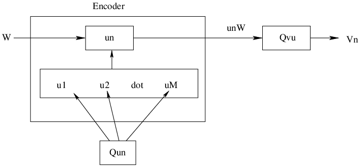
Fig. 1: Coding problem with the goal of making PVn≈QVnP_{V^{n}}\approx Q^{n}_{V}.

Consider the system depicted in Fig. 1. The random variable WW is uniformly distributed over {1,…,M}\{1,\dots,M\}, M=2n​RM=2^{nR}, and is encoded to sequences

Un=f⁡(W).\displaystyle U^{n}=f(W). (1)

VnV^{n} is generated from UnU^{n} through a memoryless channel QV|UnQ^{n}_{V|U} and has distribution PVnP_{V^{n}}. A rate RR is achievable if for any ξ>0\xi>0 there is a sufficiently large nn and an encoder such that

D(PVn||QVn)=∑vn∈supp​(PVn)P(vn)logP⁡(vn)QVn​(vn)\displaystyle D(P_{V^{n}}||Q^{n}_{V})=\sum_{v^{n}\in\text{supp}(P_{V^{n}})}P(v^{n})\log\frac{P(v^{n})}{Q^{n}_{V}(v^{n})} (2)

is less than ξ\xi. We wish to determine the smallest achievable rate.

III Main Result and Proof

Theorem 1

For a given target distribution QVQ_{V}, the rate RR is achievable if R>I⁡(V,U)R>I(V;U), where I⁡(V,U)I(V;U) is calculated with some joint distribution QU​VQ_{UV} that has marginal QVQ_{V} and |supp​(QU)|≤|𝒱||\text{supp}(Q_{U})|\leq|\mathcal{V}|. The rate RR is not achievable if R<I⁡(V,U)R<I(V;U) for all QU​VQ_{UV} with |supp​(QU)|≤|𝒱||\text{supp}(Q_{U})|\leq|\mathcal{V}|.

We provide two proofs, one with Shannon’s typicality argument and the other with Gallager’s error exponent [8] where we extend results in [3]. Suppose UU and VV have finite alphabets 𝒰\mathcal{U} and 𝒱\mathcal{V}, respectively. Let QU​VQ_{UV} be a probability distribution with marginals QUQ_{U} and QVQ_{V}. Let Un​Vn∼QU​VnU^{n}V^{n}\sim Q^{n}_{UV}, i.e., for any un∈𝒰nu^{n}\in\mathcal{U}^{n}, vn∈𝒱nv^{n}\in\mathcal{V}^{n} we have

Q⁡(un,vn)\displaystyle Q(u^{n},v^{n}) =∏i=1nQU​V​(ui,vi)=QU​Vn​(un,vn)\displaystyle=\prod^{n}_{i=1}Q_{UV}(u_{i},v_{i})=Q^{n}_{UV}(u^{n},v^{n}) (3)
Q⁡(vn|un)\displaystyle Q(v^{n}|u^{n}) =∏i=1nQV|U​(vi|ui)=QV|Un​(vn|un).\displaystyle=\prod^{n}_{i=1}Q_{V|U}(v_{i}|u_{i})=Q^{n}_{V|U}(v^{n}|u^{n}). (4)

Let 𝒞={Un​(w)}w=1M\mathcal{C}=\{U^{n}(w)\}^{M}_{w=1}, where the Un​(w),w=1,…,MU^{n}(w),w=1,\dots,M, are generated in an i.i.d. manner using QUnQ^{n}_{U}. VnV^{n} is generated from Un​(W)U^{n}(W) through the channel QV|UnQ^{n}_{V|U} (see Fig. 2). We have

P⁡(vn)=∑w=1M1M⋅QV|Un​(vn|un​(w)).\displaystyle P(v^{n})=\sum^{M}_{w=1}\frac{1}{M}\cdot Q^{n}_{V|U}(v^{n}|u^{n}(w)). (5)

Note that if for a vnv^{n} we have

QVn​(vn)=∑un∈supp​(QUn)QUn​(un)​QV|Un​(vn|un)=0\displaystyle Q^{n}_{V}(v^{n})=\sum_{u^{n}\in\text{supp}(Q^{n}_{U})}Q^{n}_{U}(u^{n})Q^{n}_{V|U}(v^{n}|u^{n})=0 (6)

then we have

QV|Un​(vn|un)=0,for all​un∈supp​(QUn).\displaystyle Q^{n}_{V|U}(v^{n}|u^{n})=0,\;\text{for all}\;u^{n}\in\text{supp}(Q^{n}_{U}). (7)

This means P⁡(vn)=0P(v^{n})=0 and supp​(PVn)⊆supp​(QVn)\text{supp}(P_{V^{n}})\subseteq\text{supp}(Q^{n}_{V}) so that D(PVn||QVn)<∞D(P_{V^{n}}||Q^{n}_{V})<\infty. We further have

E​[QV|Un​(vn|Un)QVn​(vn)]\displaystyle\text{E}\left[\frac{Q^{n}_{V|U}(v^{n}|U^{n})}{Q^{n}_{V}(v^{n})}\right] =∑unQUn​(un)⋅QV|Un​(vn|un)QVn​(vn)=1.\displaystyle=\sum_{u^{n}}Q^{n}_{U}(u^{n})\cdot\frac{Q^{n}_{V|U}(v^{n}|u^{n})}{Q^{n}_{V}(v^{n})}=1. (8)

III-A Shannon’s Typicality

The average informational divergence over WW, 𝒞\mathcal{C} and VnV^{n} is (recall that P(w)=1M,w=1,…,MP(w)=\frac{1}{M},w=1,\dots,M):

E[D(PVn||QVn)]=(a)E[log∑j=1M1M⋅QVn|Un​(Vn|Un​(j))QVn​(Vn)]\displaystyle\text{E}[D(P_{V^{n}}||Q^{n}_{V})]\overset{(a)}{=}\text{E}\left[\log\frac{\sum^{M}_{j=1}\frac{1}{M}\cdot Q_{V^{n}|U^{n}}(V^{n}|U^{n}(j))}{Q^{n}_{V}(V^{n})}\right]
=∑w=1M1M⋅E​[log⁡∑j=1MQV|Un​(Vn|Un​(j))M​QVn​(Vn)|W=w]\displaystyle=\sum^{M}_{w=1}\frac{1}{M}\cdot\text{E}\left[\log\frac{\sum^{M}_{j=1}Q^{n}_{V|U}(V^{n}|U^{n}(j))}{MQ^{n}_{V}(V^{n})}\Bigg|W=w\right]
≤(b)​∑w=1M1M⋅E​[log⁡(QV|Un​(Vn|Un​(w))M​QVn​(Vn)+M−1M)|W=w]\displaystyle\overset{(b)}{\leq}\sum^{M}_{w=1}\frac{1}{M}\cdot\text{E}\left[\log\left(\frac{Q^{n}_{V|U}(V^{n}|U^{n}(w))}{MQ^{n}_{V}(V^{n})}+\frac{M-1}{M}\right)\Bigg|W=w\right]
≤∑w=1M1M⋅E​[log⁡(QV|Un​(Vn|Un​(w))M​QVn​(Vn)+1)|W=w]\displaystyle\leq\sum^{M}_{w=1}\frac{1}{M}\cdot\text{E}\left[\log\left(\frac{Q^{n}_{V|U}(V^{n}|U^{n}(w))}{MQ^{n}_{V}(V^{n})}+1\right)\Bigg|W=w\right]
=(c)​E​[log⁡(QV|Un​(Vn|Un)M⋅QVn​(Vn)+1)]\displaystyle\overset{(c)}{=}\text{E}\left[\log\left(\frac{Q^{n}_{V|U}(V^{n}|U^{n})}{M\cdot Q^{n}_{V}(V^{n})}+1\right)\right] (9)

where

  1. (a)

    follows by taking the expectation over WW, VnV^{n} and Un​(1),…,Un​(M)U^{n}(1),\dots,U^{n}(M);

  2. (b)

    follows by the concavity of the logarithm and Jensen’s inequality applied to the expectation over the Un​(j),j≠wU^{n}(j),j\neq w, and by using (8);

  3. (c)

    follows by choosing Un​Vn∼QU​VnU^{n}V^{n}\sim Q^{n}_{UV}.

Refer to caption
Fig. 2: The random coding experiment.

Alternatively, we can make the steps (9) more explicit:

E[D(PVn||QVn)]=(a)∑un​(1)⋯∑un​(M)∏k=1MQUn(un(k))\displaystyle\text{E}[D(P_{V^{n}}||Q^{n}_{V})]\overset{(a)}{=}\sum_{u^{n}(1)}\cdots\sum_{u^{n}(M)}\prod^{M}_{k=1}{Q^{n}_{U}(u^{n}(k))}
∑vn∑w=1M1M⋅QV|Un​(vn|un​(w))​[log⁡∑j=1MQV|Un​(vn|un​(j))M⋅QVn​(vn)]\displaystyle\sum_{v^{n}}\sum^{M}_{w=1}\frac{1}{M}\cdot Q^{n}_{V|U}(v^{n}|u^{n}(w))\left[\log\frac{\sum^{M}_{j=1}Q^{n}_{V|U}(v^{n}|u^{n}(j))}{M\cdot Q^{n}_{V}(v^{n})}\right]
=∑w=1M1M​∑vn∑un​(w)QU​Vn​(un​(w),vn)\displaystyle=\sum^{M}_{w=1}\frac{1}{M}\sum_{v^{n}}\sum_{u^{n}(w)}Q^{n}_{UV}(u^{n}(w),v^{n})
∑k≠wM∑un​(k)∏l≠wMQUn​(un​(l))​[log⁡∑j=1MQV|Un​(vn|un​(j))M⋅QVn​(vn)]\displaystyle{\sum^{M}_{k\neq w}}\sum_{u^{n}(k)}{\prod^{M}_{l\neq w}}{Q^{n}_{U}(u^{n}(l))}\left[\log\frac{\sum^{M}_{j=1}Q^{n}_{V|U}(v^{n}|u^{n}(j))}{M\cdot Q^{n}_{V}(v^{n})}\right]
≤(b)​∑w=1M1M​∑vn∑un​(w)QU​Vn​(un​(w),vn)\displaystyle\overset{(b)}{\leq}\sum^{M}_{w=1}\frac{1}{M}\sum_{v^{n}}\sum_{u^{n}(w)}Q^{n}_{UV}(u^{n}(w),v^{n})
[log⁡(QV|Un​(vn|un​(w))M⋅QVn​(vn)+∑j≠wM∑un​(j)[QU​Vn​(un​(j),vn)M⋅QVn​(vn)])]\displaystyle\left[\log\left(\frac{Q^{n}_{V|U}(v^{n}|u^{n}(w))}{M\cdot Q^{n}_{V}(v^{n})}+\sum^{M}_{j\neq w}\sum_{u^{n}(j)}\left[\frac{Q^{n}_{UV}(u^{n}(j),v^{n})}{M\cdot Q^{n}_{V}(v^{n})}\right]\right)\right]
=∑w=1M1M​∑vn∑un​(w)QU​Vn​(un​(w),vn)\displaystyle=\sum^{M}_{w=1}\frac{1}{M}\sum_{v^{n}}\sum_{u^{n}(w)}Q^{n}_{UV}(u^{n}(w),v^{n})
[log⁡(QV|Un​(vn|un​(w))M⋅QVn​(vn)+M−1M)]\displaystyle\left[\log\left(\frac{Q^{n}_{V|U}(v^{n}|u^{n}(w))}{M\cdot Q^{n}_{V}(v^{n})}+\frac{M-1}{M}\right)\right]
≤∑w=1M1M​∑vn∑un​(w)QU​Vn​(un​(w),vn)\displaystyle\leq\sum^{M}_{w=1}\frac{1}{M}\sum_{v^{n}}\sum_{u^{n}(w)}Q^{n}_{UV}(u^{n}(w),v^{n})
[log⁡(QV|Un​(vn|un​(w))M⋅QVn​(vn)+1)]\displaystyle\quad\left[\log\left(\frac{Q^{n}_{V|U}(v^{n}|u^{n}(w))}{M\cdot Q^{n}_{V}(v^{n})}+1\right)\right]
=(c)​E​[log⁡(QV|Un​(Vn|Un)M⋅QVn​(Vn)+1)].\displaystyle\overset{(c)}{=}\text{E}\left[\log\left(\frac{Q^{n}_{V|U}(V^{n}|U^{n})}{M\cdot Q^{n}_{V}(V^{n})}+1\right)\right]. (10)

We remark that the identity after (a)(a) is valid for M=1M=1 by interpreting the empty sum followed by an empty product to be 11. We may write (9) or (10) as

E​[log⁡(QV|Un​(Vn|Un)M⋅QVn​(Vn)+1)]=d1+d2\displaystyle\text{E}\left[\log\left(\frac{Q^{n}_{V|U}(V^{n}|U^{n})}{M\cdot Q^{n}_{V}(V^{n})}+1\right)\right]=d_{1}+d_{2} (11)

where

d1=∑(un,vn)∈𝒯ϵn​(QU​V)Q⁡(un,vn)​log⁡(Q⁡(vn|un)M⋅Q⁡(vn)+1)\displaystyle d_{1}=\sum_{(u^{n},v^{n})\in\mathcal{T}^{n}_{\epsilon}(Q_{UV})}Q(u^{n},v^{n})\log\left(\frac{Q(v^{n}|u^{n})}{M\cdot Q(v^{n})}+1\right)
d2=∑(un,vn)∉𝒯ϵn​(QU​V)(un,vn)∈supp​(QU​Vn)​Q​(un,vn)​log⁡(Q⁡(vn|un)M⋅Q⁡(vn)+1).\displaystyle d_{2}=\underset{(u^{n},v^{n})\in\text{supp}(Q^{n}_{UV})}{\sum_{(u^{n},v^{n})\notin\mathcal{T}^{n}_{\epsilon}(Q_{UV})}}Q(u^{n},v^{n})\log\left(\frac{Q(v^{n}|u^{n})}{M\cdot Q(v^{n})}+1\right).

Using standard inequalities (see [7]) we have

d1\displaystyle d_{1} ≤∑(un,vn)∈𝒯ϵn​(QU​V)Q⁡(un,vn)​log⁡(2−n⁡(1−ϵ)​H​(V|U)M⋅2−n⁡(1+ϵ)​H​(V)+1)\displaystyle\leq\sum_{(u^{n},v^{n})\in\mathcal{T}^{n}_{\epsilon}(Q_{UV})}Q(u^{n},v^{n})\log\left(\frac{2^{-n(1-\epsilon)H(V|U)}}{M\cdot 2^{-n(1+\epsilon)H(V)}}+1\right)
≤log⁡(2−n⁡(1−ϵ)​H​(V|U)M⋅2−n⁡(1+ϵ)​H​(V)+1)\displaystyle\leq\log\left(\frac{2^{-n(1-\epsilon)H(V|U)}}{M\cdot 2^{-n(1+\epsilon)H(V)}}+1\right)
=log⁡(2−n⁡(R−I⁡(V,U)−ϵ⁡(H⁡(V|U)+H⁡(V)))+1)\displaystyle=\log\left(2^{-n(R-I(V;U)-\epsilon(H(V|U)+H(V)))}+1\right)
≤log⁡(e)⋅2−n⁡(R−I⁡(V,U)−2​ϵ​H​(V))\displaystyle\leq\log(e)\cdot 2^{-n(R-I(V;U)-2\epsilon H(V))} (12)

and d1→0d_{1}\rightarrow 0 if R>I⁡(V,U)+2​ϵ​H​(V)R>I(V;U)+2\epsilon H(V) and n→∞n\rightarrow\infty. We further have

d2\displaystyle d_{2} ≤∑(un,vn)∉𝒯ϵn​(QU​V)(un,vn)∈supp​(QU​Vn)​Q​(un,vn)​log⁡((1μV)n+1)\displaystyle\leq\underset{(u^{n},v^{n})\in\text{supp}(Q^{n}_{UV})}{\sum_{(u^{n},v^{n})\notin\mathcal{T}^{n}_{\epsilon}(Q_{UV})}}Q(u^{n},v^{n})\log\left(\left(\frac{1}{\mu_{V}}\right)^{n}+1\right)
≤2​|𝒱|⋅|𝒰|⋅e−2​n​ϵ2​μU​V2​log⁡((1μV)n+1)\displaystyle\leq 2|\mathcal{V}|\cdot|\mathcal{U}|\cdot e^{-2n\epsilon^{2}\mu^{2}_{UV}}\log\left(\left(\frac{1}{\mu_{V}}\right)^{n}+1\right) (13)
≤2​|𝒱|⋅|𝒰|⋅e−2​n​ϵ2​μU​V2⋅n⋅log⁡(1μV+1)\displaystyle\leq 2|\mathcal{V}|\cdot|\mathcal{U}|\cdot e^{-2n\epsilon^{2}\mu^{2}_{UV}}\cdot n\cdot\log\left(\frac{1}{\mu_{V}}+1\right) (14)

and d2→0d_{2}\rightarrow 0 as n→∞n\rightarrow\infty, where

μV\displaystyle\mu_{V} =minv∈supp​(QV)​Q​(v)\displaystyle=\text{min}_{v\in\text{supp}(Q_{V})}Q(v) (15)
μU​V\displaystyle\mu_{UV} =min(v,u)∈supp​(QU​V)​Q​(u,v).\displaystyle=\text{min}_{(v,u)\in\text{supp}(Q_{UV})}Q(u,v). (16)

Combining the above we have

E[D(PVn||QVn)]→0\displaystyle\text{E}[D(P_{V^{n}}||Q^{n}_{V})]\rightarrow 0 (17)

if R>I⁡(V,U)+2​ϵ​H​(V)R>I(V;U)+2\epsilon H(V) and n→∞n\rightarrow\infty. As usual, (17) means that there must exist a code with D(PVn||QVn)<ξD(P_{V^{n}}||Q^{n}_{V})<\xi for any ξ>0\xi>0 and sufficiently large nn. This proves the coding theorem. The converse follows from [1, Theorem 5.2] by removing the normalization factor 1n\frac{1}{n}.

Remark 1

The cardinality bound on supp​(QU)\text{supp}(Q_{U}). can be derived using techniques from [9, Ch. 15].

Remark 2

If V=UV=U, then we have R>H⁡(V)R>H(V).

Theorem 1 is proved using a uniform WW which represents strings of uniform bits. If we use a non-uniform WW for the coding scheme, can we still drive the unnormalized informational divergence to zero? We give the answer in the following lemma.

Lemma 1

Let W=Bn​RW=B^{nR} be a bit stream with n​RnR bits that are generated i.i.d. with a binary distribution PXP_{X} with PX​(0)=pP_{X}(0)=p, 0<p≤120<p\leq\frac{1}{2}. The rate RR is achievable if

R>I⁡(V,U)H2​(p)\displaystyle R>\frac{I(V;U)}{H_{2}(p)} (18)

where H2​(⋅)H_{2}(\cdot) is the binary entropy function.

Proof:

The proof is given in Appendix A. ∎

Remark 3

Lemma 1 states that even if WW is not uniformly distributed, the informational divergence can be made small. This is useful because if the distribution of WW is not known exactly, then we can choose RR large enough to guarantee the desired resolvability result. A similar result was developed in [4] for secrecy.

III-B Gallager’s Error Exponent

We provide a second proof using Gallager’s error exponent [8] by extending [3, Lemma 2] to asymptotic cases. Consider −12≤ρ≤0-\frac{1}{2}\leq\rho\leq 0 and define

E0n​(ρ,QU​Vn)\displaystyle E^{n}_{0}(\rho,Q^{n}_{UV}) =log⁡∑vn2⁡{E​[P​(vn)11+ρ]}1+ρ\displaystyle=\log_{2}\sum_{v^{n}}\left\{\text{E}[P(v^{n})^{\frac{1}{1+\rho}}]\right\}^{1+\rho} (19)
E0​(ρ,QU​V)\displaystyle E_{0}(\rho,Q_{UV}) =log⁡∑v2⁡{∑uQ⁡(u)​Q​(v|u)11+ρ}1+ρ\displaystyle=\log_{2}\sum_{v}\left\{\sum_{u}Q(u)Q(v|u)^{\frac{1}{1+\rho}}\right\}^{1+\rho} (20)
EG​(R,QU​V)\displaystyle E_{G}(R,Q_{UV}) =inf−12≤ρ<0{E0​(ρ,QU​V)+ρ​R}.\displaystyle=\inf_{-\frac{1}{2}\leq\rho<0}\;\left\{E_{0}(\rho,Q_{UV})+\rho R\right\}. (21)

Due to [3, Lemma 2], we have the following properties concerning E0n​(ρ,QU​Vn)E^{n}_{0}(\rho,Q^{n}_{UV}) and E0​(ρ,QU​V)E_{0}(\rho,Q_{UV}):

Property 1:

E0n​(0,QU​Vn)\displaystyle E^{n}_{0}(0,Q^{n}_{UV}) =E0​(0,QU​V)=0\displaystyle=E_{0}(0,Q_{UV})=0 (22)

Property 2:

∂E0n​(ρ,QU​Vn)∂ρ|ρ=0\displaystyle\left.\frac{\partial E^{n}_{0}(\rho,Q^{n}_{UV})}{\partial\rho}\right|_{\rho=0} =−E[D(PVn||QVn)]\displaystyle=-\text{E}[D(P_{V^{n}}||Q^{n}_{V})]
∂E0​(ρ,QU​V)∂ρ|ρ=0\displaystyle\left.\frac{\partial E_{0}(\rho,Q_{UV})}{\partial\rho}\right|_{\rho=0} =−I⁡(V,U)\displaystyle=-I(V;U) (23)

Property 3:

∂2E0n​(ρ,QU​Vn)∂ρ2\displaystyle\frac{\partial^{2}E^{n}_{0}(\rho,Q^{n}_{UV})}{\partial\rho^{2}} ≥0\displaystyle\geq 0
∂2E0​(ρ,QU​V)∂ρ2\displaystyle\frac{\partial^{2}E_{0}(\rho,Q_{UV})}{\partial\rho^{2}} ≥0\displaystyle\geq 0 (24)

Due to [8, Theorem 5.6.3], we have

{EG​(R,QU​V)<0if​R>I⁡(V,U)EG​(R,QU​V)=0if​R≤I⁡(V,U)\displaystyle\left\{\begin{array}[]{ll}E_{G}(R,Q_{UV})<0&\text{if}\;R>I(V;U)\\ E_{G}(R,Q_{UV})=0&\text{if}\;R\leq I(V;U)\end{array}\right.

By extending [3, Sec. III, Inequality (15)] to asymptotic cases, we have the following lemma.

Lemma 2

We have

E0n​(ρ,QU​Vn)≤log2⁡(1+2n​EG​(R,QU​V)).\displaystyle E^{n}_{0}(\rho,Q^{n}_{UV})\leq\log_{2}\left(1+2^{nE_{G}(R,Q_{UV})}\right). (27)
Proof:

The proof is given in Appendix B.

Refer to caption
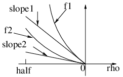
Fig. 3: An example of E0n​(ρ,QU​Vn)E^{n}_{0}(\rho,Q^{n}_{UV}) and E0​(ρ,QU​V)E_{0}(\rho,Q_{UV}).

∎Combining Properties 11-33, we have E0n​(ρ,QU​Vn)E^{n}_{0}(\rho,Q^{n}_{UV}) and E0​(ρ,QU​V)E_{0}(\rho,Q_{UV}) are convex in ρ\rho, for −12≤ρ≤0-\frac{1}{2}\leq\rho\leq 0 and (see Fig. 3)

ρ⋅(−E[D(PVn||QVn)])\displaystyle\rho\cdot(-\text{E}[D(P_{V^{n}}||Q^{n}_{V})]) ≤E0n​(ρ,QU​Vn)\displaystyle\leq E^{n}_{0}(\rho,Q^{n}_{UV}) (28)

which means

E[D(PVn||QVn)]\displaystyle\text{E}[D(P_{V^{n}}||Q^{n}_{V})] ≤E0n​(ρ,QU​Vn)−ρ\displaystyle\leq\frac{E^{n}_{0}(\rho,Q^{n}_{UV})}{-\rho}
≤(a)​log2⁡(1+2n​EG​(R,QU​V))−ρ\displaystyle\overset{(a)}{\leq}\frac{\log_{2}\left(1+2^{nE_{G}(R,Q_{UV})}\right)}{-\rho} (29)

where (a)(a) follows from Lemma 2. The right hand side of (29) goes to 00 as n→∞n\rightarrow\infty as long as (see (III-B))

R>I⁡(V,U).\displaystyle R>I(V;U). (30)
Remark 4

This proof applies to continuous random variables by replacing the sums in the proof of Lemma 2 with integrals.

Remark 5

The average divergence E[D(PVn||QVn)]\text{E}[D(P_{V^{n}}||Q^{n}_{V})] can be viewed as the mutual information I⁡(𝒞,Vn)I(\mathcal{C};V^{n}) from the random codebook 𝒞\mathcal{C} to the output VnV^{n} [3, Sec. III]. To show this, denote 𝒞~\mathcal{\widetilde{C}} as a realization of 𝒞\mathcal{C} and we have (see (10))

I⁡(𝒞,Vn)=∑𝒞~P⁡(𝒞~)​∑vnP⁡(vn|𝒞~)​log⁡P⁡(vn|𝒞~)QVn​(vn)\displaystyle I(\mathcal{C};V^{n})=\sum_{\mathcal{\widetilde{C}}}P(\mathcal{\widetilde{C}})\sum_{v^{n}}P(v^{n}|\mathcal{\widetilde{C}})\log\frac{P(v^{n}|\mathcal{\widetilde{C}})}{Q^{n}_{V}(v^{n})}
=∑un​(1)⋯∑un​(M)∏k=1MQUn(un(k))\displaystyle=\sum_{u^{n}(1)}\cdots\sum_{u^{n}(M)}\prod^{M}_{k=1}Q^{n}_{U}(u^{n}(k))
∑vn∑w=1M1M⋅QV|Un​(vn|un​(w))​log⁡∑j=1M1M​QV|Un​(vn|un​(j))QVn​(vn)\displaystyle\sum_{v^{n}}\sum^{M}_{w=1}\frac{1}{M}\cdot Q^{n}_{V|U}(v^{n}|u^{n}(w))\log\frac{\sum^{M}_{j=1}\frac{1}{M}Q^{n}_{V|U}(v^{n}|u^{n}(j))}{Q^{n}_{V}(v^{n})}
=E​[log⁡∑j=1M1M​QV|Un​(Vn|Un​(j))QVn​(Vn)]\displaystyle=\text{E}\left[\log\frac{\sum^{M}_{j=1}\frac{1}{M}Q^{n}_{V|U}(V^{n}|U^{n}(j))}{Q^{n}_{V}(V^{n})}\right]
=E[D(PVn||QVn)].\displaystyle=\text{E}[D(P_{V^{n}}||Q^{n}_{V})]. (31)

Thus, as E[D(PVn||QVn)]→0\text{E}[D(P_{V^{n}}||Q^{n}_{V})]\rightarrow 0 we have I⁡(𝒞,Vn)→0I(\mathcal{C};V^{n})\rightarrow 0 which means that 𝒞\mathcal{C} and VnV^{n} are (almost) independent. This makes sense, since as PVn→QVnP_{V^{n}}\rightarrow Q^{n}_{V} one is not able to distinguish which codebook is used to generate the output.

IV Discussion

Hayashi studied the resolvability problem using unnormalized divergence and he derived bounds for nonasymptotic cases [3, Lemma 2]. We have outlined his proof steps in Sec. III-B. Theorem 1 can be derived by extending [3, Lemma 2] to asymptotic cases (see III-B) and it seems that such a result was the underlying motivation for [3, Lemma 2]. Unfortunately, Theorem 1 is not stated explicitly in [3] and the ensuing asymptotic analysis was done for normalized informational divergence. Hayashi’s proofs (he developed two approaches) were based on Shannon random coding.

Theorem 1 implies [1, Theorem 6.3] which states that for R>I⁡(V,U)R>I(V;U) the normalized divergence 1nD(PVn||QVn)\frac{1}{n}D(P_{V^{n}}||Q^{n}_{V}) can be made small. Theorem 1 implies [2, Theorem 4] for product distributions through Pinsker’s inequality [10, Lemma 11.6.1]

D(PX||QX)≥12​ln⁡2||PX−QX||TV2\displaystyle D(P_{X}||Q_{X})\geq\frac{1}{2\ln 2}||P_{X}-Q_{X}||^{2}_{\text{TV}} (32)

where

‖PX−QX‖TV=∑x|P⁡(x)−Q⁡(x)|.\displaystyle||P_{X}-Q_{X}||_{\text{TV}}=\sum_{x}|P(x)-Q(x)|. (33)

Moreover, the speed of decay in (12) and (14) is (almost) exponential with nn. We can thus make

α(n)⋅E[D(PVn||QVn)]\displaystyle\alpha(n)\cdot\text{E}\left[D(P_{V^{n}}||Q^{n}_{V})\right] (34)

vanishingly small as n→∞n\rightarrow\infty, where α⁡(n)\alpha(n) represents a sub-exponential function of nn that satisfies,

limn→∞n⋅α⁡(n)eβ​n=0\displaystyle\lim_{n\rightarrow\infty}\frac{n\cdot\alpha(n)}{e^{\beta n}}=0 (35)

where β\beta is positive and independent of nn (see also [3]). For example, we may choose α⁡(n)=nm\alpha(n)=n^{m} for any integer mm. We may also choose α⁡(n)=eγ​n\alpha(n)=e^{\gamma n} where γ<β\gamma<\beta.

Since all achievability results in [11] are based on [2, Theorem 4], Theorem 1 extends the results in [11] as well. Theorem 1 is closely related to strong secrecy [12] and provides a simple proof that Shannon random coding suffices to drive an unnormalized mutual information between messages and eavesdropper observations to zero.

Theorem 1 is valid for approximating product distributions only. However extensions to a broader class of distributions, e.g., information stable distributions [2], are clearly possible.

Finally, an example code is as follows (courtesy of F. Kschischang). Consider a channel with input and output alphabet the 272^{7} binary 77-tuples. Suppose the channel maps each input uniformly to a 77-tuple that is distance 00 or 11 away, i.e., there are 88 channel transitions for every input and each transition has probability 18\frac{1}{8}. A simple “modulation” code for this channel is the (7,4)(7,4) Hamming code. The code is perfect and if we choose each codeword with probability 116\frac{1}{16}, then the output V7V^{7} of the channel is uniformly distributed over all 272^{7} values. Hence I⁡(V,U)=4I(V;U)=4 bits suffice to “approximate”  the product distribution (here there is no approximation).

Appendix A Non-Uniform WW

Observe that H⁡(W)=H⁡(Bn​R)=n​R⋅H2​(p)H(W)=H(B^{nR})=nR\cdot H_{2}(p). Following the same steps as in (9) we have

E[D(PVn||QVn)]=E[log∑j=1MP⁡(j)​QVn|Un​(Vn|Un​(j))QVn​(Vn)]\displaystyle\text{E}[D(P_{V^{n}}||Q^{n}_{V})]=\text{E}\left[\log\frac{\sum^{M}_{j=1}P(j)Q_{V^{n}|U^{n}}(V^{n}|U^{n}(j))}{Q^{n}_{V}(V^{n})}\right]
=∑wP⁡(w)⋅E​[log⁡∑j=1MP⁡(j)​QV|Un​(Vn|Un​(j))QVn​(Vn)|W=w]\displaystyle=\sum_{w}P(w)\cdot\text{E}\left[\log\frac{\sum^{M}_{j=1}P(j)Q^{n}_{V|U}(V^{n}|U^{n}(j))}{Q^{n}_{V}(V^{n})}\Bigg|W=w\right]
≤∑wP⁡(w)⋅E​[log⁡(P⁡(w)​QV|Un​(Vn|Un​(w))QVn​(Vn)+1−P⁡(w))]\displaystyle\leq\sum_{w}P(w)\cdot\text{E}\left[\log\left(\frac{P(w)Q^{n}_{V|U}(V^{n}|U^{n}(w))}{Q^{n}_{V}(V^{n})}+1-P(w)\right)\right]
≤∑wP⁡(w)⋅E​[log⁡(P⁡(w)​QV|Un​(Vn|Un​(w))QVn​(Vn)+1)]\displaystyle\leq\sum_{w}P(w)\cdot\text{E}\left[\log\left(\frac{P(w)Q^{n}_{V|U}(V^{n}|U^{n}(w))}{Q^{n}_{V}(V^{n})}+1\right)\right]
=d1+d2+d3\displaystyle=d_{1}+d_{2}+d_{3} (36)

where

d1\displaystyle d_{1} =∑w∈𝒯ϵn​(PXn)P⁡(w)​∑(un​(w),vn)∈𝒯ϵn​(QU​Vn)QU​Vn​(un​(w),vn)\displaystyle=\sum_{w\in\mathcal{T}^{n}_{\epsilon}(P^{n}_{X})}P(w)\sum_{(u^{n}(w),v^{n})\in\mathcal{T}^{n}_{\epsilon}(Q^{n}_{UV})}Q^{n}_{UV}(u^{n}(w),v^{n})
[log⁡(P⁡(w)​QV|Un​(vn|un​(w))QVn​(vn)+1)]\displaystyle\quad\quad\left[\log\left(\frac{P(w)Q^{n}_{V|U}(v^{n}|u^{n}(w))}{Q^{n}_{V}(v^{n})}+1\right)\right]
d2\displaystyle d_{2} =∑w∈𝒯ϵn​(PXn)P⁡(w)​∑(un​(w),vn)∉𝒯ϵn​(QU​V)(un​(w),vn)∈supp​(QU​Vn)​QU​Vn​(un​(w),vn)\displaystyle=\sum_{w\in\mathcal{T}^{n}_{\epsilon}(P^{n}_{X})}P(w)\underset{(u^{n}(w),v^{n})\in\text{supp}(Q^{n}_{UV})}{\sum_{(u^{n}(w),v^{n})\notin\mathcal{T}^{n}_{\epsilon}(Q_{UV})}}Q^{n}_{UV}(u^{n}(w),v^{n})
[log⁡(P⁡(w)​QV|Un​(vn|un​(w))QVn​(vn)+1)]\displaystyle\quad\quad\left[\log\left(\frac{P(w)Q^{n}_{V|U}(v^{n}|u^{n}(w))}{Q^{n}_{V}(v^{n})}+1\right)\right]
d3\displaystyle d_{3} =∑w∉𝒯ϵn​(PXn)w∈supp​(PXn)​P​(w)​∑(un​(w),vn)∈supp​(QU​Vn)QU​Vn​(un​(w),vn)\displaystyle=\underset{w\in\text{supp}(P^{n}_{X})}{\sum_{w\notin\mathcal{T}^{n}_{\epsilon}(P^{n}_{X})}}P(w)\sum_{(u^{n}(w),v^{n})\in\text{supp}(Q^{n}_{UV})}Q^{n}_{UV}(u^{n}(w),v^{n})
[log⁡(P⁡(w)​QV|Un​(vn|un​(w))QVn​(vn)+1)].\displaystyle\quad\quad\left[\log\left(\frac{P(w)Q^{n}_{V|U}(v^{n}|u^{n}(w))}{Q^{n}_{V}(v^{n})}+1\right)\right]. (37)

We can bound d1d_{1} as follows (see (12))

d1\displaystyle d_{1} ≤∑w∈𝒯ϵn​(PXn)P⁡(w)​[log⁡(2n⁡(I⁡(V,U)+2​ϵ​H​(V))2n⁡(1−ϵ)​R⋅H2​(p)+1)]\displaystyle\leq\sum_{w\in\mathcal{T}^{n}_{\epsilon}(P^{n}_{X})}P(w)\left[\log\left(\frac{2^{n(I(V;U)+2\epsilon H(V))}}{2^{n(1-\epsilon)R\cdot H_{2}(p)}}+1\right)\right]
≤log⁡(2−n⁡(R⋅H2​(p)−I⁡(V,U)−ϵ⁡(2​H​(V)+R⋅H2​(p)))+1)\displaystyle\leq\log\left(2^{-n\left(R\cdot H_{2}(p)-I(V;U)-\epsilon(2H(V)+R\cdot H_{2}(p))\right)}+1\right)
≤log⁡(e)⋅2−n⁡(R⋅H2​(p)−I⁡(V,U)−δϵ​(n))\displaystyle\leq\log(e)\cdot 2^{-n\left(R\cdot H_{2}(p)-I(V;U)-\delta_{\epsilon}(n)\right)} (38)

which goes to zero if R>I⁡(V,U)+δϵ​(n)H2​(p)R>\frac{I(V;U)+\delta_{\epsilon}(n)}{H_{2}(p)} and n→∞n\rightarrow\infty, where δϵ​(n)=ϵ⁡(2​H​(V)+R⋅H2​(p))\delta_{\epsilon}(n)=\epsilon(2H(V)+R\cdot H_{2}(p)). We also have

d2\displaystyle d_{2} ≤∑w∈𝒯ϵn​(PXn)P⁡(w)​∑(un​(w),vn)∉𝒯ϵn​(QU​V)(un​(w),vn)∈supp​(QU​Vn)​QU​Vn​(un​(w),vn)\displaystyle\leq\sum_{w\in\mathcal{T}^{n}_{\epsilon}(P^{n}_{X})}P(w)\underset{(u^{n}(w),v^{n})\in\text{supp}(Q^{n}_{UV})}{\sum_{(u^{n}(w),v^{n})\notin\mathcal{T}^{n}_{\epsilon}(Q_{UV})}}Q^{n}_{UV}(u^{n}(w),v^{n})
[log⁡((1μV)n+1)]\displaystyle\quad\quad\left[\log\left(\left(\frac{1}{\mu_{V}}\right)^{n}+1\right)\right]
≤2​|𝒱|⋅|𝒰|⋅e−2​n​ϵ2​μU​V2​log⁡((1μV)n+1)\displaystyle\leq 2|\mathcal{V}|\cdot|\mathcal{U}|\cdot e^{-2n\epsilon^{2}\mu^{2}_{UV}}\log\left(\left(\frac{1}{\mu_{V}}\right)^{n}+1\right) (39)

which goes to zero as n→∞n\rightarrow\infty (see (14)). We further have

d3\displaystyle d_{3} ≤∑w∉𝒯ϵn​(PXn)w∈supp​(PXn)​P​(w)​∑(un​(w),vn)∈supp​(QU​Vn)QU​Vn​(un​(w),vn)\displaystyle\leq\underset{w\in\text{supp}(P^{n}_{X})}{\sum_{w\notin\mathcal{T}^{n}_{\epsilon}(P^{n}_{X})}}P(w)\sum_{(u^{n}(w),v^{n})\in\text{supp}(Q^{n}_{UV})}Q^{n}_{UV}(u^{n}(w),v^{n})
[log⁡((1μV)n+1)]\displaystyle\quad\quad\left[\log\left(\left(\frac{1}{\mu_{V}}\right)^{n}+1\right)\right]
≤∑w∉𝒯ϵn​(PXn)w∈supp​(PXn)​P​(w)​[log⁡((1μV)n+1)]\displaystyle\leq\underset{w\in\text{supp}(P^{n}_{X})}{\sum_{w\notin\mathcal{T}^{n}_{\epsilon}(P^{n}_{X})}}P(w)\left[\log\left(\left(\frac{1}{\mu_{V}}\right)^{n}+1\right)\right]
≤4⋅e−2​n​ϵ2​p2​log⁡((1μV)n+1)\displaystyle\leq 4\cdot e^{-2n\epsilon^{2}p^{2}}\log\left(\left(\frac{1}{\mu_{V}}\right)^{n}+1\right) (40)

which goes to zero as n→∞n\rightarrow\infty (see (14)).

Combining the above for non-uniform WW we have

E[D(PVn||QVn)]→0\displaystyle\text{E}[D(P_{V^{n}}||Q^{n}_{V})]\rightarrow 0 (41)

if R>I⁡(V,U)+δn​(ϵ)H2​(p)R>\frac{I(V;U)+\delta_{n}(\epsilon)}{H_{2}(p)} and n→∞n\rightarrow\infty.

Appendix B Proof of Lemma 2

We extend the proof of [3, Sec. III, Inequality (15)] to asymptotic cases to establish Lemma 2. Recall that −12≤ρ≤0-\frac{1}{2}\leq\rho\leq 0. Let s=−ρ1+ρs=\frac{-\rho}{1+\rho} so we have

0≤s≤1\displaystyle 0\leq s\leq 1
1+s=11+ρ\displaystyle 1+s=\frac{1}{1+\rho} (42)

We also have for any a,b≥0a,b\geq 0 and 0≤x≤10\leq x\leq 1

(a+b)x≤ax+bx.\displaystyle(a+b)^{x}\leq a^{x}+b^{x}. (43)

Observe that for any vnv^{n} we have

E​[P​(vn)]\displaystyle\text{E}[P(v^{n})] =E​[∑w=1M1M⋅QV|Un​(vn|Un​(w))]\displaystyle=\text{E}\left[\sum^{M}_{w=1}\frac{1}{M}\cdot Q^{n}_{V|U}(v^{n}|U^{n}(w))\right]
=E​[QV|Un​(vn|Un​(1))]\displaystyle=\text{E}\left[Q^{n}_{V|U}(v^{n}|U^{n}(1))\right]
=E​[∏i=1nQV|U​(vi|Ui​(1))]\displaystyle=\text{E}\left[\prod^{n}_{i=1}Q_{V|U}(v_{i}|U_{i}(1))\right]
=∏i=1nE​[QV|U​(vi|Ui​(1))]\displaystyle=\prod^{n}_{i=1}\text{E}\left[Q_{V|U}(v_{i}|U_{i}(1))\right]
=∏i=1n[∑uQ⁡(u)​QV|U​(vi|u)]\displaystyle=\prod^{n}_{i=1}\left[\sum_{u}Q(u)Q_{V|U}(v_{i}|u)\right]
=∏i=1nQV​(vi)=QVn​(vn)\displaystyle=\prod^{n}_{i=1}Q_{V}(v_{i})=Q^{n}_{V}(v^{n}) (44)

We further have

2E0n​(ρ,QU​Vn)=∑vn{E​[P​(vn)11+ρ]}1+ρ\displaystyle 2^{E^{n}_{0}(\rho,Q^{n}_{UV})}=\sum_{v^{n}}\left\{\text{E}[P(v^{n})^{\frac{1}{1+\rho}}]\right\}^{1+\rho}
=(a)​∑vn{E​[P​(vn)1+s]}11+s\displaystyle\overset{(a)}{=}\sum_{v^{n}}\left\{\text{E}[P(v^{n})^{1+s}]\right\}^{\frac{1}{1+s}}
=∑vn{E​[(∑w=1M1M⋅QV|Un​(vn|Un​(w)))1+s]}11+s\displaystyle=\sum_{v^{n}}\left\{\text{E}\left[\left(\sum^{M}_{w=1}\frac{1}{M}\cdot Q^{n}_{V|U}(v^{n}|U^{n}(w))\right)^{1+s}\right]\right\}^{\frac{1}{1+s}}
=1M∑vn{E[∑w=1MQV|Un(vn|Un(w))\displaystyle=\frac{1}{M}\sum_{v^{n}}\left\{\text{E}\left[\sum^{M}_{w=1}Q^{n}_{V|U}(v^{n}|U^{n}(w))\right.\right.
(QV|Un(vn|Un(w))+∑j≠wMQV|Un(vn|Un(j)))s]}11+s\displaystyle\left.\left.\left(Q^{n}_{V|U}(v^{n}|U^{n}(w))+\sum^{M}_{j\neq w}Q^{n}_{V|U}(v^{n}|U^{n}(j))\right)^{s}\right]\right\}^{\frac{1}{1+s}} (45)

where (a)(a) follows from (42). Applying (43) to (45) we have

2E0n​(ρ,QU​Vn)≤1M∑vn{E[∑w=1MQV|Un(vn|Un(w))\displaystyle 2^{E^{n}_{0}(\rho,Q^{n}_{UV})}\leq\frac{1}{M}\sum_{v^{n}}\left\{\text{E}\left[\sum^{M}_{w=1}Q^{n}_{V|U}(v^{n}|U^{n}(w))\right.\right.
((QV|Un(vn|Un(w)))s+(∑j≠wMQV|Un(vn|Un(j)))s)]}11+s\displaystyle\left.\left.\left(\left(Q^{n}_{V|U}(v^{n}|U^{n}(w))\right)^{s}+\left(\sum^{M}_{j\neq w}Q^{n}_{V|U}(v^{n}|U^{n}(j))\right)^{s}\right)\right]\right\}^{\frac{1}{1+s}}
=(a)1M∑vn{E[∑w=1M(QV|Un(vn|Un(w)))1+s]\displaystyle\overset{(a)}{=}\frac{1}{M}\sum_{v^{n}}\left\{\text{E}\left[\sum^{M}_{w=1}\left(Q^{n}_{V|U}(v^{n}|U^{n}(w))\right)^{1+s}\right]\right.
+∑w=1M(E[QV|Un(vn|Un(w))])\displaystyle\quad\quad\quad\quad\quad\quad+\sum^{M}_{w=1}\left(\text{E}\left[Q^{n}_{V|U}(v^{n}|U^{n}(w))\right]\right)
⋅E[(∑j≠wMQV|Un(vn|Un(j)))s]}11+s\displaystyle\left.\quad\quad\quad\quad\quad\quad\cdot\text{E}\left[\left(\sum^{M}_{j\neq w}Q^{n}_{V|U}(v^{n}|U^{n}(j))\right)^{s}\right]\right\}^{\frac{1}{1+s}}
≤(b)1M∑vn{ME[(QV|Un(vn|Un))1+s]\displaystyle\overset{(b)}{\leq}\frac{1}{M}\sum_{v^{n}}\left\{M\text{E}\left[\left(Q^{n}_{V|U}(v^{n}|U^{n})\right)^{1+s}\right]\right.
+MQVn(vn)⋅(E[∑j≠wMQV|Un(vn|Un(j))])s}11+s\displaystyle\left.+MQ^{n}_{V}(v^{n})\cdot\left(\text{E}\left[\sum^{M}_{j\neq w}Q^{n}_{V|U}(v^{n}|U^{n}(j))\right]\right)^{s}\right\}^{\frac{1}{1+s}}
=(c)1M∑vn{ME[(QV|Un(vn|Un))1+s]\displaystyle\overset{(c)}{=}\frac{1}{M}\sum_{v^{n}}\left\{M\text{E}\left[\left(Q^{n}_{V|U}(v^{n}|U^{n})\right)^{1+s}\right]\right.
+MQVn(vn)((M−1)QVn(vn))s}11+s\displaystyle\left.\quad\quad+MQ^{n}_{V}(v^{n})\left((M-1)Q^{n}_{V}(v^{n})\right)^{s}\right\}^{\frac{1}{1+s}}
≤1M​∑vn{M​E​[(QV|Un​(vn|Un))1+s]+(M​QVn​(vn))1+s}11+s\displaystyle\leq\frac{1}{M}\sum_{v^{n}}\left\{M\text{E}\left[\left(Q^{n}_{V|U}(v^{n}|U^{n})\right)^{1+s}\right]+\left(MQ^{n}_{V}(v^{n})\right)^{1+s}\right\}^{\frac{1}{1+s}} (46)

where

  1. (a)

    follows because Un​(w)U^{n}(w) is independent of Un​(j)U^{n}(j), j≠wj\neq w

  2. (b)

    follows by choosing Un​Vn∼QU​VnU^{n}V^{n}\sim Q^{n}_{UV}, by the concavity of xax^{a} for 0≤a≤10\leq a\leq 1 and by (44)

  3. (c)

    follows by (44)

Applying (43) again to (46) we have

2E0n​(ρ,QU​Vn)≤1M∑vn{(ME[(QV|Un(vn|Un))1+s])11+s\displaystyle 2^{E^{n}_{0}(\rho,Q^{n}_{UV})}\leq\frac{1}{M}\sum_{v^{n}}\left\{\left(M\text{E}\left[\left(Q^{n}_{V|U}(v^{n}|U^{n})\right)^{1+s}\right]\right)^{\frac{1}{1+s}}\right.
+MQVn(vn)}\displaystyle\left.\quad\quad\quad\quad\quad\quad\quad\quad\quad\quad+MQ^{n}_{V}(v^{n})\right\}
=(a)​1+Mρ​∑vn(E​[(QV|Un​(vn|Un))11+ρ])1+ρ\displaystyle\overset{(a)}{=}1+M^{\rho}\sum_{v^{n}}\left(\text{E}\left[\left(Q^{n}_{V|U}(v^{n}|U^{n})\right)^{\frac{1}{1+\rho}}\right]\right)^{1+\rho}
=1+Mρ​∑vn(∑unQUn​(un)​(QV|Un​(vn|un))11+ρ)1+ρ\displaystyle=1+M^{\rho}\sum_{v^{n}}\left(\sum_{u^{n}}Q^{n}_{U}(u^{n})\left(Q^{n}_{V|U}(v^{n}|u^{n})\right)^{\frac{1}{1+\rho}}\right)^{1+\rho}
=(b)​1+2n​ρ​R​∑v(∑uQ⁡(u)​(Q⁡(v|u))11+ρ)n⁡(1+ρ)\displaystyle\overset{(b)}{=}1+2^{n\rho R}\sum_{v}\left(\sum_{u}Q(u)\left(Q(v|u)\right)^{\frac{1}{1+\rho}}\right)^{n(1+\rho)}
=1+2n⁡(E0​(ρ,QU​V)+ρ​R)\displaystyle=1+2^{n(E_{0}(\rho,Q_{UV})+\rho R)} (47)

where

  1. (a)

    follows from (42)

  2. (b)

    follows because the Ui​ViU_{i}V_{i} are i.i.d., i=1,…,ni=1,\dots,n

Optimizing over ρ\rho, we have

E0n​(ρ,QU​Vn)≤log2⁡(1+2n​EG​(R,QU​V)).\displaystyle E^{n}_{0}(\rho,Q^{n}_{UV})\leq\log_{2}\left(1+2^{nE_{G}(R,Q_{UV})}\right). (48)

Acknowledgment

J. Hou and G. Kramer were supported by an Alexander von Humboldt Professorship endowed by the German Federal Ministry of Education and Research. G. Kramer was also supported by NSF Grant CCF-09-05235. The authors thank G. Böcherer, F. Kschischang and M. Bloch for useful remarks.

References

  • [1] A. Wyner, “The common information of two dependent random variables,” IEEE Trans. Inf. Theory, vol. 21, no. 2, pp. 163–179, March 1975.
  • [2] T. Han and S. Verdú, “Approximation theory of output statistics,” IEEE Trans. Inf. Theory, vol. 39, no. 3, pp. 752–772, May 1993.
  • [3] M. Hayashi, “General nonasymptotic and asymptotic formulas in channel resolvability and identification capacity and their application to the wiretap channel,” IEEE Trans. Inf. Theory, vol. 52, no. 4, pp. 1562–1575, April 2006.
  • [4] M. Bloch and J. Kliewer, “On secure communication with constrained randomization,” in IEEE Int. Symp. Inf. Theory, Boston, MA, USA, 2012, pp. 1172–1176.
  • [5] I. Csiszár, “Almost independence and secrecy capacity,” Prob. of Inf. Transmission, vol. 32, no. 1, pp. 40–47, Jan.–March 1996.
  • [6] J. L. Massey, Applied Digital Information Theory, ETH Zurich, Zurich, Switzerland, 1980-1998.
  • [7] A. Orlitsky and J. Roche, “Coding for computing,” IEEE Trans. Inf. Theory, vol. 47, no. 3, pp. 903–917, March 2001.
  • [8] R. G. Gallager, Information Theory and Reliable Communication. Wiley, 1968.
  • [9] I. Csiszár and J. Körner, Information Theory: Coding Theorems for Discrete Memoryless Systems. New York: Academic, 1981.
  • [10] T. Cover and J. Thomas, Elements of Information Theory, 2nd ed. New York: Wiley, 2006.
  • [11] P. Cuff, H. Permuter, and T. Cover, “Coordination capacity,” IEEE Trans. Inf. Theory, vol. 56, no. 9, pp. 4181–4206, Sept. 2010.
  • [12] M. Bloch and J. Barros, Physical Layer Security From Information Theory to Security Engineering. Cambridge University Press, 2011.