Rank regularization and Bayesian inference
for tensor completion and extrapolation†
Abstract
A novel regularizer of the PARAFAC decomposition factors capturing the tensor’s rank is proposed in this paper, as the key enabler for completion of three-way data arrays with missing entries. Set in a Bayesian framework, the tensor completion method incorporates prior information to enhance its smoothing and prediction capabilities. This probabilistic approach can naturally accommodate general models for the data distribution, lending itself to various fitting criteria that yield optimum estimates in the maximum-a-posteriori sense. In particular, two algorithms are devised for Gaussian- and Poisson-distributed data, that minimize the rank-regularized least-squares error and Kullback-Leibler divergence, respectively. The proposed technique is able to recover the “ground-truth” tensor rank when tested on synthetic data, and to complete brain imaging and yeast gene expression datasets with and of missing entries respectively, resulting in recovery errors at dB and dB.
Index Terms:
Tensor, low-rank, missing data, Bayesian inference, Poisson process.I Introduction
Imputation of missing data is a basic task arising in various Big Data applications as diverse as medical imaging [12], bioinformatics [3], as well as social and computer networking [10, 17]. The key idea rendering recovery feasible is the “regularity” present among missing and available data. Low rank is an attribute capturing this regularity, and can be readily exploited when data are organized in a matrix. A natural approach to low-rank matrix completion problem is minimizing the rank of a target matrix, subject to a constraint on the error in fitting the observed entries [4]. Since rank minimization is generally NP-hard [26], the nuclear norm has been advocated recently as a convex surrogate to the rank [11]. Beyond tractability, nuclear-norm minimization enjoys good performance both in theory as well as in practice [4].
The goal of this paper is imputation of missing entries of tensors (also known as multi-way arrays), which are high-order generalizations of matrices frequently encountered in chemometrics, medical imaging, and networking [16, 8]. Leveraging the low-rank structure for tensor completion is challenging, since even computing the tensor rank is NP-hard [14]. Defining a nuclear norm surrogate is not obvious either, since singular values as defined by the Tucker decomposition are not generally related with the rank. Traditional approaches to finding low-dimensional representations of tensors include unfolding the multi-way data and applying matrix factorizations such as the singular-value decomposition (SVD) [7, 25, 3] or, employing the parallel factor (PARAFAC) decomposition [24, 9]. In the context of tensor completion, an approach falling under the first category can be found in [12], while imputation using PARAFAC was dealt with in [2].
The imputation approach presented in this paper builds on a novel regularizer accounting for the tensor rank, that relies on redefining the matrix nuclear norm in terms of its low-rank factors. The contribution is two-fold. First, it is established that the low-rank inducing property of the regularizer carries over to tensors by promoting sparsity in the factors of the tensor’s PARAFAC decomposition. In passing, this analysis allows for drawing a neat connection with the atomic-norm in [5]. The second contribution is the incorporation of prior information, with a Bayesian approach that endows tensor completion with extra smoothing and prediction capabilities. A parallel analysis in the context of reproducing kernel Hilbert spaces (RKHS) further explains these acquired capabilities, provides an alternative means of obtaining the prior information, and establishes a useful connection with collaborative filtering approaches [1] when reduced to the matrix case.
While least-squares (LS) is typically utilized as the fitting criterion for matrix and tensor completion, implicitly assuming Gaussian data, the adopted probabilistic framework supports the incorporation of alternative data models. Targeting count processes available in the form of network traffic data, genome sequencing, and social media interactions, which are modeled as Poisson distributed, the maximum a posteriori (MAP) estimator is expressed in terms of the Kullback-Leibler (K-L) divergence [10].
The remainder of the paper is organized as follows. Section II offers the necessary background on nuclear-norm regularization for matrices, the PARAFAC decomposition, and the definition of tensor rank. Section III presents the tensor completion problem, establishing the low-rank inducing property of the proposed regularization. Prior information is incorporated in Section IV, with Bayesian and RKHS formulations of the tensor imputation method, leading to the low-rank tensor-imputation (LRTI) algorithm. Section V develops the method for Poisson tensor data, and redesigns the algorithm to minimize the rank-regularized K-L divergence. Finally, Section VI presents numerical tests carried out on synthetic and real data, including expression levels in yeast, and brain magnetic resonance images (MRI). Conclusions are drawn in Section VII, while most technical details are deferred to the Appendix.
The notation adopted throughout includes bold lowercase and capital letters for vectors and matrices , respectively, with superscript denoting transposition. Tensors are underlined as e.g., , and their slices carry a subscript as in ; see also Fig. 1. Both the matrix and tensor Frobenius norms are represented by . Symbols , , and denote the Kroneker, Kathri-Rao, Hadamard (entry-wise), and outer product, respectively.
II Preliminaries
II-A Nuclear-norm minimization for matrix completion
Low-rank approximation is a popular method for estimating missing values of a matrix , which capitalizes on “regularities” across the data [11]. For the imputation to be feasible, a binding assumption that relates the available entries with the missing ones is required. An alternative is to postulate that has low rank . The problem of finding matrix with rank not exceeding , which approximates in the given entries specified by a binary matrix , can be formulated as
| (1) |
The low-rank property of matrix implies that the vector of its singular values is sparse. Hence, the rank constraint is equivalent to where the -(pseudo)norm equals the number of nonzero entries of its vector argument.
Aiming at a convex relaxation of the NP-hard problem (1), one can leverage recent advances in compressive sampling [11] and surrogate the -norm with the -norm, which here equals the nuclear norm of defined as . With this relaxation, the Lagrangian counterpart of (1) is
| (2) |
where is a rank-controlling parameter. Problem (2) can be further transformed by considering the following characterization of the nuclear norm [23]
| (3) |
For an arbitrary matrix with SVD , the minimum in (3) is attained for and . The optimization in (3) is over all possible bilinear factorizations of , so that the number of columns of and is also a variable. Building on (3), one can arrive at the following equivalent reformulation of (2) [17]
| (4) |
The equivalence implies that by finding the global minimum of (4), one can recover the optimal solution of (2). However, since (4) is nonconvex, it may have multiple stationary points. Interestingly, the next result provides conditions for these stationary points to be globally optimal (parts a) and b) are proved in the Appendix, while the proof for c) can be found in [17].)
II-B PARAFAC decomposition
The PARAFAC decomposition of a tensor is at the heart of the proposed imputation method, since it offers a means to define its rank [24, 9]. Given , consider matrices , , and , such that
| (5) |
The rank of is the minimum value of for which this decomposition is possible. For , the PARAFAC decomposition is given by the corresponding factor matrices (all with columns), so that (5) holds with .

To appreciate why the aforementioned rank definition is natural, rewrite (5) as , where , , and represent the -th columns of , , and , respectively; and the outer products have entries The rank of a tensor is thus the minimum number of outer products (rank one factors) required to represent the tensor. It is not uncommon to adopt an equivalent normalized representation
| (6) |
by defining unit-norm vectors , , , and weights , .
Let denote the -th slice of along its third (tube) dimension, such that ; see Fig. 1. The following compact form of the PARAFAC decomposition in terms of slice factorizations will be used in the sequel
| (7) |
where the diagonal matrix has the vector on its diagonal, and is the -th row of the identity matrix. The PARAFAC decomposition is symmetric [cf. (5)], and one can also write , or, in terms of slices along the first (row), or, second (column) dimensions.
III Rank regularization for tensors
Generalizing the nuclear-norm regularization technique (2) from low-rank matrix to tensor completion is not straightforward, since singular values of a tensor (given by the Tucker decomposition) are not related to the rank [16]. Fortunately, the Frobenius-norm regularization outlined in Section II-A offers a viable option for low-rank tensor completion under the PARAFAC model, by solving
| (8) |
where the Frobenius norm of a tensor is defined as , and the Hadamard product as .
Different from the matrix case, it is unclear whether the regularization in (8) bears any relation with the tensor rank. Interestingly, the following analysis corroborates the capability of (8) to produce a low-rank tensor , for sufficiently large . In this direction, consider an alternative completion problem stated in terms of the normalized tensor representation (6)
| (9) |
where ; the nonconvex (pseudo)-norm is given by ; and the unit-norm constraint on the factors’ columns is left implicit. Problems (8) and (9) are equivalent as established by the following proposition (its proof is provided in the Appendix.)
Proposition 2: The solutions of (8) and (9) coincide, i.e., , with optimal factors related by , , and , .
To further stress the capability of (8) to produce a low-rank approximant tensor , consider transforming (9) once more by rewriting it in the constrained-error form
| (10) | ||||
For any value of there exists a corresponding Lagrange multiplier such that (9) and (10) yield the same solution, under the identity . [Since is an increasing function, the exponent of can be safely eliminated without affecting the minimizer of (10).] The -norm in (10) produces a sparse vector when minimized [6], sharing this well-documented property of the -norm as their norm-one balls, depicted in Fig. 2, share the “pointy geometry” which is responsible for inducing sparsity.
With (8) equivalently rewritten as in (10), its low-rank inducing property is now revealed. As in (10) becomes sparse, some of its entries are zeroed, and the corresponding outer-products drop from the sum in (6), thus lowering the rank of .
The next property is a direct consequence of the low-rank promoting property of (8) as established in Proposition III.
Corollary 1: If denotes the solution to problem (8) , and , then .
Corollary III asserts that if the penalty parameter is chosen large enough, the rank is reduced to the extreme case . To see why this is a non-trivial property, it is prudent to think of ridge-regression estimates where similar quadratic regularizers are adopted, but an analogous property does not hold. In ridge regression one needs to let in order to obtain an all-zero solution. Characterization of is also of practical relevance as it provides a frame of reference for tuning the regularization parameter.
Using (10), it is also possible to relate (8) with the atomic norm in [5]. Indeed, the infimum -norm of is a proper norm for , named atomic norm, and denoted by [5]. Thus, by replacing with , (10) becomes convex in . Still, the complexity of solving such a variant of (10) resides in that is generally intractable to compute [5]. In this regard, it is remarkable that arriving to (10) had the sole purpose of demonstrating the low-rank inducing property, and that (8) is to be solved by the algorithm developed in the ensuing section. Such an algorithm will neither require computing the atomic norm or PARAFAC decomposition of , nor knowing its rank. The number of columns in , , and can be set to an overestimate of the rank of , such as the upper bound , and the low-rank of will be induced by regularization as argued earlier. To carry out a fair comparison, only convergence to a stationary point of (8) will be guaranteed in this paper.
Remark 1: These insights foster future research directions for the design of a convex regularizer of the tensor rank. Specifically, substituting for the regularization term in (8), turns into in the equivalent (10). It is envisioned that with such a modification in place, the acquired convexity of (10) would enable a reformulation of Proposition II-A, providing conditions for global optimality of the stationary points of (8).

Still, a limitation of (8) is that it does not allow for incorporating side information that could be available in addition to the given entries .
Remark 2: In the context of recommender systems, a description of the users and/or products through attributes (e.g., gender, age) or measures of similarity, is typically available. It is thus meaningful to exploit both known preferences and descriptions to model the preferences of users [1]. In three-way (samples, genes, conditions) microarray data analysis, the relative position of single-nucleotide polymorphisms in the DNA molecule implies degrees of correlation among genotypes [22]. These correlations could be available either through a prescribed model, or, through estimates obtained using a reference tensor . A probabilistic approach to tensor completion capable of incorporating such types of extra information is the subject of the ensuing section.
IV Bayesian low-rank tensor approximation
IV-A Bayesian PARAFAC model
A probabilistic approach is developed in this section in order to integrate the available statistical information into the tensor imputation setup. To this end, suppose that the observation noise is zero-mean, white, Gaussian; that is
| (11) |
Since vectors in (6) are interchangeable, identical distributions are assigned across and they are modeled as independent from each other, zero-mean Gaussian distributed with covariance matrix . Similarly, vectors and are uncorrelated and zero-mean, Gaussian, with covariance matrix and , respectively. In addition , , and are assumed mutually uncorrelated. And since scale ambiguity is inherently present in the PARAFAC model, vectors , , and are set to have equal power; that is,
| (12) |
Under these assumptions, the negative of the posterior distribution can be readily written as , with
Correspondingly, the MAP estimator of is
| (13) |
reducing to (8) when and This Bayesian approach interprets the regularization parameter [cf. (8)] as the noise variance, which is useful in practice to select . The ensuing section explores the advantages of incorporating prior information to the imputation method.
IV-B Nonparametric tensor decomposition
Incorporating the information conveyed by , , and , together with a practical means of finding these matrices can be facilitated by interpreting (13) in the context of RKHS [27]. In particular, the analysis presented next will use the Representer Theorem, interpreted as an instrument for finding the best interpolating function in a Hilbert space spanned by kernels, just as interpolation with sinc-kernels is carried out in the space of bandlimited functions for the purpose of reconstructing a signal from its samples [19].
In this context, it is instructive to look at a tensor as a function of three variables and , living in measurable spaces and , respectively. Generalizing (8) to this nonparametric framework, low-rank functions are formally defined to belong to the following family
where , , and are Hilbert spaces constructed from specified kernels , and , defined over , , and , while is an initial overestimate of the rank of .
The following nonparametric fitting criterion is adopted for finding the best interpolating data
| (14) |
It is shown in the Appendix that leveraging the Representer Theorem, the minimizer of (14) admits a finite dimensional representation in terms of , and ,
| (15) |
where vector and matrix have entries , ; and where , , , and are correspondingly defined in terms of and . It is also shown in the Appendix that the coefficient matrices , , and can be found by solving
| (16) |
Problem (16) reduces to (8) when the side information is discarded by selecting , and as Kronecker deltas, in which case , , and are identity matrices. In the general case, (16) yields the sought nonlinear low-rank approximation method for when combined with (15), evidencing the equivalence between (14) and (13).
Interpreting (14) as an interpolator renders (13) a natural choice for tensor imputation, where in general, missing entries are to be inserted by connecting them to surrounding points on the three-dimensional arrangement. Relative to (8), this RKHS perspective also highlights (13)’s extra smoothing and extrapolation capabilities. Indeed, by capitalizing on the similarities captured by , and , (16) can recover completely missing slices. This feature is not shared by imputation methods that leverage low-rank only, since these require at least one point in the slice to build on colinearities. Extrapolation is also possible in this sense. If for instance can be expanded to capture a further point not in the original set, then a new slice of data can be predicted by (15) based on its correlation with the available entries. These extra capabilities will be exploited in Section VI, where correlations are leveraged for the imputation of MRI data. The method described by (13) and (16) can be applied to matrix completion by just setting entries of to one, and can be extended to higher-order dimensions with a straightforward alteration of the algorithms and theorems throughout this paper.
Identification of covariance matrices , , and with kernel matrices , and is the remaining aspect to clarify in the connection between (13) and (16). It is apparent from (13) and (16) that correlations between columns of the factors are reflected in similarities between the tensor slices, giving rise to the opportunity of obtaining one from the other. This aspect is explored next.
IV-C Covariance estimation
To implement (13), matrices , , and must be postulated a priori, or alternatively replaced by their sample estimates. Such estimates need a training set of vectors , , and abiding to the Bayesian model just described, and this requires PARAFAC decomposition of training data. In order to abridge this procedure, it is convenient to inspect how , , and are related to their kernel counterparts.
Based on the equivalence between the standard RKHS interpolator and the linear mean-square error estimator [21], it is useful to re-visit the probabilistic framework and identify kernel similarities between slices of with their mutual covariances. Focusing on the tube dimension of , one can write , that is, the covariance between slices and taking as the standard inner product in the matrix space. Under this alternative definition for , and corresponding definitions for , and , it is shown in the Appendix that
| (17) |
and that is related to the second-order moment of by
| (18) |
Since sample estimates for , , , and can be readily obtained from the tensor data, (17) and (18) provide an agile means of estimating , , and without requiring PARAFAC decompositions over the set of training tensors.
This strategy remains valid when kernels are not estimated from data. One such case emerges in collaborative filtering of user preferences [1], where the similarity of two users is modeled as a function of attributes; such age or income.
IV-D Block successive upper-bound minimization algorithm
An iterative algorithm is developed here for solving (13), by cyclically minimizing the cost over , , and . In the first step of the cycle the cost in (13) is minimized with respect to (w.r.t.) considering and as parameters. Accordingly, the partial cost to minimize reduces to
| (19) |
where was identified with and substituted for . Function (19) is quadratic in and can be readily minimized after re-writing it in terms of [see (55) in the Appendix]. However, such an approach becomes computationally infeasible for other than small datasets, since it involves storing matrices of dimensions , and solving a linear system of equations. The alternative pursued here to overcome this obstacle relies on the so-called block successive upper-bound minimization (BSUM) algorithm [20].
In BSUM one minimizes a judiciously chosen upper-bound of , which: i) depends on the current iterate ; ii) should be simpler to optimize; and iii) satisfies certain local-tightness conditions; see also [20] and properties i)-iii) below.
For given, consider the function
| (20) | ||||
where is the maximum eigenvalue of , and . The following properties of imply that it majorizes at , satisfying the technical conditions required for the convergence of BSUM (properties i)-iii) are established in the the proof of Lemma V-A in the Appendix).
- i)
;
- ii)
; and,
- iii)
.
The computational advantage of minimizing in place of comes from being separable across rows of . To see this, consider the Kathri-Rao product , defined by the column-wise Kronecker products . Let also matrix denote the unfolding of along its tube dimension, and likewise for and . Then, using the following identity [10]
| (21) |
it is possible to rewrite (20) as
which can be decomposed as
| (22) |
where , , , , and , represent the -th rows of matrices , , , , and , respectively. Not only (22) evidences the separability of (20) across rows of , but it also presents each of its summands in a standardized quadratic form that can be readily minimized by equating its gradient to zero. Accordingly, the majorization strategy reduces the computational load to systems of equations that can be solved in parallel. Collecting the solution of such quadratic programs into the rows of a matrix yields the minimizer of (20), and the update for the BSUM cycle. Such a procedure is presented in Algorithm 1, where analogous updates for and are carried out cyclically.
V Inference for low-rank Poisson tensors
Adoption of the LS criterion in (8) assumes in a Bayesian setting that the random is Gaussian distributed. This section deals with a Poisson-distributed tensor , a natural alternative to the Gaussian model when integer-valued data are obtained by counting independent events [10]. Suppose that the entries of are Poisson distributed, with probability mass function
| (23) |
and means given by the corresponding entries in tensor . For mutually-independent , the log-likelihood of given data only on the entries specified by , takes the form
| (24) |
after dropping terms that do not depend on .
The choice of the Poisson distribution in (23) over a Gaussian one for counting data, prompts minimization of the K-L divergence (24) instead of LS as a more suitable criterion [10]. Still, the entries of are not coupled in (24), and a binding PARAFAC modeling assumption is natural for feasibility of the tensor approximation task under missing data. Mimicking the method for Gaussian data, (nonnegative) Gaussian priors are assumed for the factors of the PARAFAC decomposition. Accordingly, the MAP estimator of given Poisson-distributed data (entries of indexed by ) becomes
| (25) |
over the feasible set , where the symbol should be understood to imply entry-wise nonegativity.
With the aid of Representer’s Theorem, it is also possible to interpret (25) as a variational estimator in RKHS, with K-L analogues to (14)-(16), so that the conclusions thereby regarding smoothing, prediction and prior covariance estimation carry over to the low-rank Poisson imputation method (25).
V-A Block successive upper-bound minimization algorithm
A K-L counterpart of the LRTI algorithm is developed in this section, that provably converges to a stationary point of (25), via an alternating-minimization iteration which optimizes (25) sequentially w.r.t. one factor matrix, while holding the others fixed.
In the sequel, the goal is to arrive at a suitable expression for the cost in (25), when viewed only as a function of e.g., . To this end, let matrix denote the unfolding of along its tube dimension, and likewise for and . Based on these definitions, (24) can be written as
| (26) |
where , are all-one vectors of dimensions and respectively, and should be understood entry-wise. The log-likelihood in (26) can be expressed in terms of , and the Kathri-Rao product by resorting again to (21). Substituting (21) into (26) one arrives at the desired expression for the cost in (25) as a function of , namely
A closed-form minimizer for is not available, but since is convex one could in principle resort to an iterative procedure to obtain . To avoid extra inner iterations, the approach here relies again on the BSUM algorithm [20].
For given, consider the separable function
| (27) |
where is the largest eigenvalue of , and the parameters , , and are defined in terms of , , and by
and , with As asserted in the following lemma, majorizes at and satisfies the technical conditions required for the convergence of BSUM (see the Appendix for a proof.)
Lemma 1: Function satisfies the following properties
- i)
;
- ii)
; and,
- iii)
.
Moreover, is minimized at with entries .
Lemma V-A highlights the reason behind adopting in the proposed block-coordinate descent algorithm: it is separable across the entries of its matrix argument [cf. (27)], and hence it admits a closed-form minimizer given by the scalars . The updates are tabulated under Algorithm 2 for solving (25), where analogous updates for and are carried out cyclically.
By virtue of properties i)-iii) in Lemma V-A, convergence of Algorithm 2 follows readily from the general convergence theory available for the BSUM algorithm [20].
Proposition 4: The iterates for , and generated by Algorithm 2 converge to a stationary point of (25).
A related algorithm, abbreviated as CP-APR can be found in [10], where the objective is to find the tensor’s low-rank factors per se. The LRPTI algorithm here generalizes CP-APR by focusing on recovering missing data, and incorporating prior information through rank regularization. In terms of convergence to a stationary point, the added regularization allows for lifting the assumption on the linear independence of the rows of , as required by CP-APR [10] - an assumption without a straightforward validation since iterates are not accessible beforehand.
VI Numerical Tests
VI-A Simulated Gaussian data
Synthetic tensor-data of dimensions were generated according to the Bayesian tensor model described in Section IV. Specifically, entries of consist of realizations of Gaussian random variables generated according to (11), with means specified by entries of and variance scaled to yield an SNR of dB . Tensor is constructed from factors , and as in (7). Matrices , and have columns containing realizations of independent zero-mean, unit-variance, Gaussian random variables.
A quarter of the entries of were removed at random and reserved to evaluate performance. The remaining seventy five percent of the data were used to recover considering the removed data as missing entries. Method (8) was employed for recovery, as implemented by the LRTI Algorithm, with regularization resulting from setting , , and .
The relative recovery error between and data was computed, along with the rank of the recovered tensor, as a measure of performance. Fig. 3 depicts these figures of merit averaged over repetitions of the experiment, across values of varying on the interval to , which is computed as in Corollary III.


Fig 3 (bottom) shows that the LRTI algorithm is successful in recovering the missing entries of up to dB for a wide range of values of , presenting a minimum at . This result is consistent with Fig. 3 (top), which shows that rank is approximately recovered at the minimum error. Fig. 3 (top) also corroborates the low-rank inducing effect of (8), with the recovered rank varying from the upper bound to , as is increased, and confirms that the recovered tensor is null at as asserted by Corollary III.
VI-B Simulated Poisson data
The synthetic example just described was repeated for the low-rank Poisson-tensor model described in Section V. Specifically, tensor data of dimensions were generated according to the low-rank Poisson-tensor model of Section V. Entries of consist of realizations of Poisson random variables generated according to (23), with means specified by entries of . Tensor is again constructed as in (7) from factors , and having columns, containing the absolute value of realizations of independent Gaussian random variables scaled to yield . Half of the entries of were considered missing to be recovered from the remaining half. Method (25) was employed for recovery, as implemented by the LRPTI Algorithm, with regularization .
Fig. 4 shows the estimated rank and recovery error over realizations of the experiment, for in the interval to .

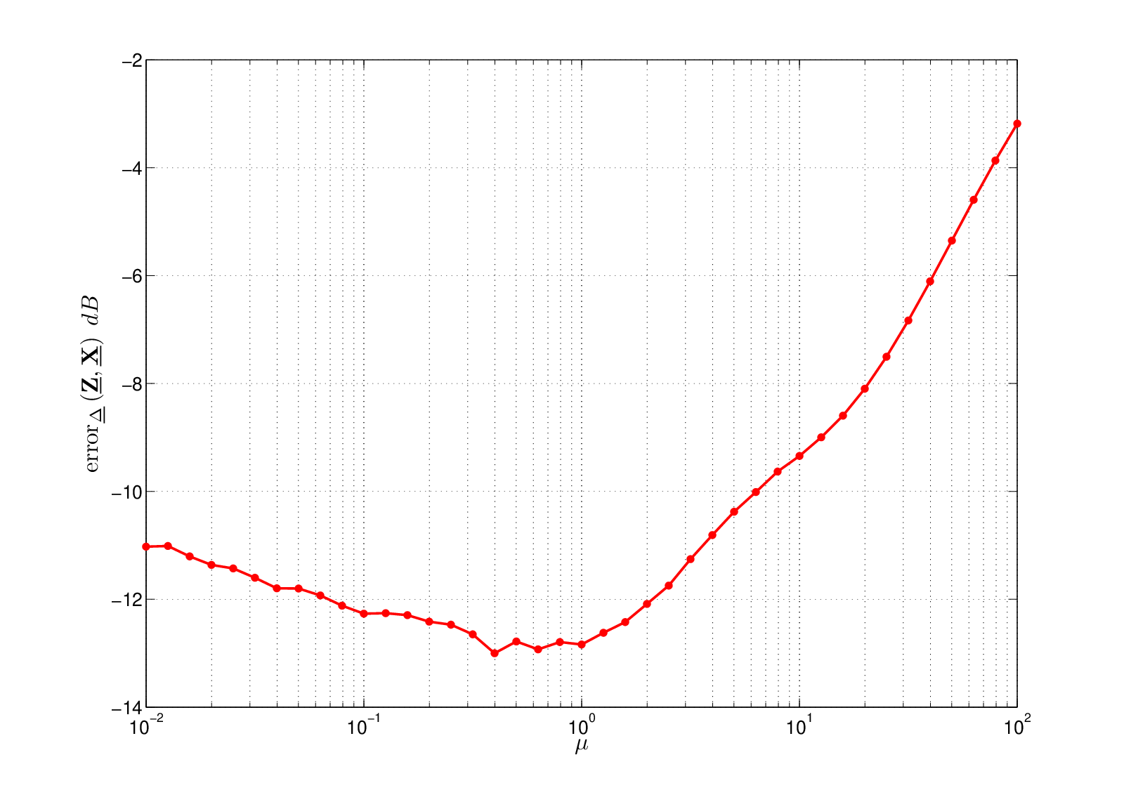
The recovery error in Fig. 4 (bottom) exhibits a minimum of dB at , where the rank is recovered [cf. Fig. 4 (top).] The low-rank inducing effect of (8) is again corroborated by the decreasing trend in Fig. 4 (top), but in this case the rank is lower bounded by , because the K-L fitting criterion prevents (25) from yielding a null estimate .
VI-C MRI data
Estimator (14) was tested against a corrupted version of the MRI brain data set 657 from the Internet brain segmentation repository [15]. The tensor to be estimated corresponds to a three-dimensional MRI scan of the brain comprising a set of images, each of pixels. Fifty percent of the data is removed uniformly at random together with the whole slice . Fig. 5 depicts the results of applying estimator (14) to the remaining data, which yields a reconstruction error of dB. The original slice , its corrupted counterpart, and the resulting estimate are shown on top and center left. Covariance matrices , and are estimated from six additional tensor samples containing complementary scans of the brain also available at [15]. Fig. 5 (center right) represents the covariance matrix for column slices perpendicular to , showing a structure that reflects symmetries of the brain. This correlation is the key enabler for the method to recover the missing slice up to dB (see Fig. 5 (bottom)) by interpolating its a priori similar parallel counterparts.
All in all, the experiment evidences the merits of low-rank PARAFAC decomposition for modeling a tensor, the ability of the Bayesian estimator (13) in recovering missing data, and the usefulness of incorporating correlations as side information.
On account of the comprehensive analysis of three-way MRI data arrays in [8], and the nonnegative PARAFAC decomposition advanced thereby, inference of tensors with nonnegative continuous entries will be pursued as future research, combining methods and algorithms in sections IV and V of this paper.


VI-D RNA sequencing data
The RNA-Seq method described in [18] exhaustively counts the number of RNA transcripts from yeast cells. The reverse transcription of RNA molecules into cDNA is achieved by alternative methods, differentiated by the use of oligo-dT, or random-hexonucleotide primers. These cDNA molecules are sequenced to obtain counts of RNA molecules across genes on the yeast genome. The experiment was repeated in [18] for a biological and a technological replicate of the original sample totalling instances per primer selection. The data are thus organized in a tensor of dimensions as shown in Fig. 6 (top), with integer data that are modeled as Poisson counts. Fifteen percent of the data is removed and reserved for assessing performance. The missing data are represented in white in Fig. 6 (center).


VII Concluding summary
It was shown in this paper that regularizing with the Frobenius-norm square of the PARAFAC decomposition factors, controls the tensor’s rank by inducing sparsity in the vector of amplitudes of its rank-one components. A Bayesian method for tensor completion was developed based on this property, introducing priors on the tensor factors. It was argued, and corroborated numerically, that this prior information endows the completion method with extra capabilities in terms of smoothing and extrapolation. It was also suggested through a parallelism between Bayesian and RKHS inference, that the prior covariance matrices can be obtained from (sample) correlations among the tensor’s slices. In such a probabilistic context, generic distribution models for the data lead to multiple fitting criteria. Gaussian and Poisson processes were especially considered by developing algorithms that minimize the regularized LS and K-L divergence, respectively.
Numerical tests on synthetic data corroborated the low-rank inducing property, and the ability of the completion method to recover the “ground-truth” rank, while experiments with brain images and gene expression levels in yeast served to evaluate the method’s performance on real datasets.
Although the results and algorithms in this paper were presented for three-way arrays, they are readily extendible to higher-order tensors or reducible to the matrix case.
I. Proof of Proposition II-A
Proof:
a) The equivalence of (2) and (4) results immediately from (3). Indeed, if (4) is minimized in two steps
| (28) |
it is apparent that the LS part of the cost does not depend on the inner minimization variables. Hence, (28) can be rewritten as
| (29) |
and by recognizing (3) as the inner problem in (29), the equivalence follows.
b) Consider the cost in (4) at the local minimum
where . Arguing by contradiction, suppose that there is a different local minimum such that , and without loss of generality set , so that , which can be expanded to
| (30) |
Setting this inequality aside for now, consider the augmented matrix in terms of generic and matrices:
and the corresponding defined in terms of and .
For each value of consider the convex combination
| (36) |
As both and are positive semi-definite, so is and by means of the Choleski factorization one obtains
which defines , and .
Expanding the cost difference as in (30) results in
From the definitions (VII)-(VII) it follows that , , and , so that
and thus, it can be put in terms of (30) as in
If were strictly negative, so would , and hence
but then there is in every neighborhood of a point such that , cannot be a local minimum. This contradiction implies that for any pair of local minima, which proves the statement in part b) of Proposition II-A. ∎ II-Equivalence of tensor completion problems
Proof:
The Frobenius square-norms of , , and are separable across columns; hence, the penalty in (8) can be rewritten as
| (42) |
by defining , , , .
On the other hand, can be expressed w.l.o.g. in terms of the normalized outer products (6) with . Substituting (6) and (42) for the tensor and the penalty respectively, (8) reduces to
| (43) |
Focusing on the inner minimization w.r.t. norms , , and for arbitrary fixed directions , , and , and fixed products . The constraints and hence the LS part of the cost depend on only, and not on their particular factorizations . Thus, the penalty is the only term that varies when is constant, rendering the inner-most minimization in (43) equivalent to
| (44) | ||||
The arithmetic geometric-mean inequality gives the solution to (44), as it states that for scalars , and , it holds that
with equality when , so that the minimum of (44) is attained at .
Substituting the corresponding into (43) yields (9). Equivalence of the optimization problems is transitive; hence, by showing that both (9) and (8) equivalent to (43) proves them equivalent to each other, as desired. ∎
III. Proof of Corollary III
Proof:
The following result on the norm of the matrix inverse will be used in the proof of the corollary.
Lemma 2: [13, p.58] If satisfies , then is invertible, and
Another useful inequality holds for any value of , and for , , and being the minimizers of (8)
| (45) |
as it follows from comparing the cost at such a minimum, and at the feasible point .
A second characterization of the minimum of (8) will be obtained by equating the gradient to zero. By vectorizing matrix , the cost in (8) can be rewritten as
| (46) |
where , , and denote the vector rearrangements of matrices , , and , respectively. Additional regularization that vanishes when taking derivatives w.r.t. were removed from (46). Setting the gradient of (46) w.r.t. to zero, yields
with
The norms of and can be bounded by using the sub-multiplicative property of the norm, and the Cauchy-Schwarz inequality, which results in
Then according to the previous lemma, if is chosen large enough so that then the norm of is bounded by
| (47) |
which constitutes the sought second characterization of the minimum of (8).
Yet a third characterization was obtained during the proof of Proposition III, in which the norm of the factor columns were shown equal to each other, so that
| (48) |
Form (50), two cases are found possible:
| case 1: | ||||
| case 2: | (51) |
To argue that the second case is impossible, substitute (49) into (51) and square the result to obtain
| (52) |
But by hypothesis so that , and the right-hand side of (52) is bounded by , so that the inequality does not hold. This implies that the first case in (51); i.e., , must hold, which in accordance with (48), further implies a null solution of (8). That was the object of this proof. Still, the bound at can be pushed to one by further reducing , and the proof remains valid under the slightly relaxed condition . ∎ IV-RKHS imputation
Recursive application of Representer’s Theorem yields finite dimensional representations for the minimizers , , and of (14), given by
Defining vectors , and correspondingly , and , along with matrices , , and , it follows that
| (53) |
Matrices , and are further obtained by solving
which is transformed into (16) by changing variables , , and , just as (53) becomes (15).
V-Covariance estimation
Inspection of the entries of under the PARAFAC model, yields
which, after summing over , yields
| (54) |
In addition, by incorporating the equal power assumption (12), equation (54) further simplifies to
as stated in (18).
VI - Vector form of (19)
The vec operator can be combined with the Kronecker product to factorize , and with the Hadamard product to convert it to a standard matrix product . Using these two properties, (19) can be put in terms of as in
| (55) |
VII - Proof of Lemma V-A
Proof:
Function in (27) is formed from after substituting for , and for , respectively, as defined by
| (56) | ||||
| (57) |
where and , and
| (58) | ||||
| (59) |
with
Hence, properties i)-iii) will be satisfied by the pair of functions and in Lemma V-A, as long as they are satisfied both by the pair in (56)-(57) and that in (58)-(59).
Focusing on the first pair, both functions are separable per column of and , and their difference takes the form
which is positive and, together with its gradient, vanish at . This establishes that properties i)-iii) are satisfied by and , and thus they are so for functions and in (20) and (19).
Considering the second pair, and expanding yields
| (60) |
where the logarithm can be rewritten as (see also [10])
| (61) | |||
| (62) |
and the inequality holds because of the concavity of the logarithm with an argument being a convex combination with coefficients summing up to one.
Since substituting (62) for (61) in (60) results in (59), it follows that and satisfy property iii). The proof is complete after evaluating at the pair of functions and their derivatives at to confirm that properties i) and ii) hold too.
The minimum is obtained readily after equating to zero the derivative of the corresponding summand in (22), and selecting the nonnegative root. ∎
References
- [1] J. Abernethy, F. Bach, T. Evgeniou, and J.P. Vert. “A new approach to collaborative filtering: Operator estimation with spectral regularization,” J. of Machine Learning Research, vol. 10, pp.803-826, 2009.
- [2] E. Acar, D. M. Dunlavy, T. G. Kolda, and M. Mørup, “Scalable tensor factorizations for incomplete data,” Chemometrics and Intelligent Laboratory Systems, vol. 106, no. 1, pp. 41-56, 2011.
- [3] O. Alter, P. O. Brown, and D. Botstein, “Singular value decomposition for genome-wide expression data processing and modeling,” Proc. of the Natl. Academy of Science, vol. 97, no. 18, pp. 10101-10106, 2000.
- [4] E. J. Candes and Y. Plan, “Matrix completion with noise,” Proceedings of the IEEE, vol. 98, pp. 925–936, June 2010.
- [5] V. Chandrasekaran, B. Recht, P. A. Parrilo, and A. S. Willsky, “The convex geometry of linear inverse problems,” Foundations of Computational Mathematics, vol. 12, no. 6, Dec. 2012.
- [6] R. Chartrand, “Exact reconstruction of sparse signals via nonconvex minimization,” IEEE Signal Processing Letters, vol. 14, no. 10, pp. 707-710, Oct. 2007.
- [7] J. Chen, and Y. Saad, “On the tensor SVD and the optimal low-rank othogonal approximation of tensors,” SIAM Journal on Matrix Analysis and Applications (SIMAX), vol. 30, no. 4, pp. 1709-1734, 2009.
- [8] A. Cichocki, R. Zdunek, A.-H. Phan, and S. Amari, Nonnegative Matrix and Tensor Factorizations: Applications to Exploratory Multi-way Data Analysis, John Wiley, 2009.
- [9] J. Kruskal, “Three-way arrays: Rank and uniqueness of trilinear decompositions, with application to arithmetic complexity and statistics,” Lin. Alg. Applicat., vol. 18, no. 2, pp. 95138, 1977.
- [10] E. C. Chi and T. G. Kolda, “On tensors, sparsity, and nonnegative factorizations,” SIAM Journal on Matrix Analysis and Applications, Dec. 2012 (to appear; see also arXiv:1112.2414v3 [math.NA]).
- [11] M. Fazel, “Matrix rank minimization with applications” PhD Thesis, Electrical Engineering Dept., Stanford University, vol. 54, pp. 1-130, 2002.
- [12] S. Gandy, B. Recht, and I. Yamada, “Tensor completion and low-n-rank tensor recovery via convex optimization,” Inverse Problems, vol. 27, no. 2, pp. 1-19, 2011.
- [13] G. Golub and C. F. Van Loan, Matrix Computations, Johns Hopkins University Press, 3rd Edition, Oct. 1996.
- [14] J. Håstad, “Tensor rank is NP-complete,” J. Algorithms, vol. 11, no. 4, pp. 644-654, 1990.
- [15] Internet brain segmentation repository, “MR brain data set 657,” Center for Morphometric Analysis at Massachusetts General Hospital, available at http://www.cma.mgh.harvard.edu/ibsr/.
- [16] T. G. Kolda and B. W. Bader, “Tensor decompositions and applications,” SIAM Review, vol. 51, no. 3, pp. 455-500, 2009.
- [17] M. Mardani, G. Mateos, and G. B. Giannakis, “In-network sparsity-regularized rank minimization: Algorithms and applications,” IEEE Trans. Signal Process., 2012 arXiv:1203.1570v1 [cs.MA]).
- [18] U. Nagalakshmi et al., “The transcriptional landscape of the yeast genome defined by RNA sequencing” Science, vol. 320, no. 5881, pp. 1344-1349, June 2008.
- [19] M. Z. Nashed and Q. Sun, “Function spaces for sampling expansions,” Multiscale Signal Analysis and Modelling, edited by X. Shen and A. Zayed, Lecture Notes in EE, Springer, pp. 81-104, 2012.
- [20] M. Razaviyayn, M. Hong, and Z.-Q. Luo, “A unified convergence analysis of block successive minimization methods for nonsmooth optimization,” SIAM J. Opt., 2012; see also arXiv:1209.2385v1 [math.OC]).
- [21] C. E. Rasmussen and C. K. I. Williams, Gaussian Processes for Machine Learning, the MIT Press, 2006.
- [22] P. Scheet, and M. Stephens, “A fast and flexible statistical model for large-scale population genotype data: Applications to inferring missing genotypes and haplotypic phase,” American Journal of Human Genetics, vol. 78, pp. 629-644, 2006.
- [23] N. Srebro, J. D. M. Rennie, and T. S. Jaakkola, “Maximum-margin matrix factorization,” Advances in Neural Information Processing Systems, vol. 17, pp. = 1329-1336, 2005.
- [24] J. M. F. ten Berge and N. D. Sidiropoulos, “On uniqueness in CANDECOMP/PARAFAC,” Psychometrika, vol. 67, no. 3, pp. 399-409, 2002.
- [25] R. Tomioka, K. Hayashi, and H. Kashima, “Estimation of low-rank tensors via convex optimization,” submited 2011, also available at ArXiv:1010.0789v2 [stat.ML].
- [26] L. Vandenberghe and S. Boyd, “Semidefinite programming,” SIAM Review, vol. 38, no. 1, pp. 49-95, 1996.
- [27] G. Wahba, Spline Models for Observational Data, SIAM, PA 1990.