Robust Phase Estimation of Squeezed State

The phase $\phi(t)$ of the continuous optical phase-squeezed beam is modulated with an OU noise process, such that

where $\lambda^{-1}$ is the correlation time of $\phi(t)$, $\kappa$ determines the magnitude of the phase variation and $\nu(t)$ is a zero-mean white Gaussian noise with unity amplitude.

The phase-modulated beam is measured by homodyne detection using a local oscillator, the phase of which is adapted with the filtered estimate $\phi_{f}(t)$, thereby yielding a normalized homodyne output current $I(t)$,

where $|\alpha|$ is the amplitude of the input phase-squeezed beam, and $dW(t)$ is Wiener noise arising from squeezed vacuum fluctuations. The parameter $\bar{R}_{sq}$ is determined by the degree of squeezing ($r_{m}\geq 0$) and anti-squeezing ($r_{p}\geq r_{m}$) and by $\sigma_{f}^{2}=\langle[\phi(t)-\phi_{f}(t)]^{2}\rangle$. We use the measurement appropriately scaled as our measurement model,

where $\omega(t)=\frac{dW(t)}{dt}$ is another zero-mean white Gaussian noise with unity amplitude.

We employ the robust fixed-interval smoothing technique from Ref. [6] as used in Ref. [4]. We introduce uncertainties $\delta_{1}$ and $\delta_{2}$, respectively, in the parameters $\lambda$ and $2|\alpha|/\sqrt{\bar{R}_{sq}}$, such that Eq. (2.5) in Ref. [6] takes the form:

where $\Delta_{1}=\left[\begin{array}[]{cc}\delta_{1}&0\end{array}\right],\Delta_{2}=\left[\begin{array}[]{cc}0&\delta_{2}\end{array}\right],|\delta_{1}|\leq 1,|\delta_{2}|\leq 1,K=\left[\begin{array}[]{c}-\mu\lambda/\sqrt{\kappa}\\ 2\mu|\alpha|/\sqrt{\bar{R}_{sq}}\end{array}\right]$. $0\leq\mu<1$ is the level of uncertainty. $\Delta_{1}$ and $\Delta_{2}$ satisfy: $||[\begin{array}[]{cc}\Delta_{1}^{\prime}Q^{1\over 2}&\Delta_{2}^{\prime}R^{1\over 2}\end{array}]||\leq 1$, such that $Q=R=1$. The IQC of Eq. (2.4) in Ref. [6] for our model is:

where $z=K\phi$ is the uncertainty output, and $w=\Delta_{1}K\phi+\nu$ and $v=\Delta_{2}K\phi+\omega$ are the uncertainty inputs.

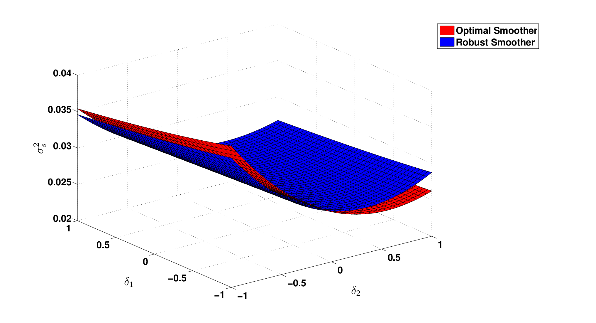
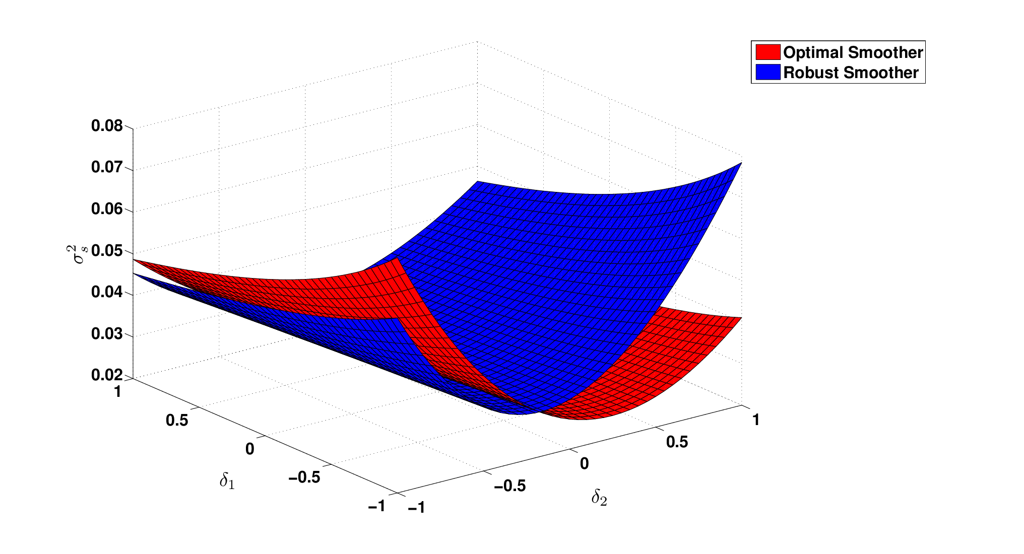
We use the method from Ref. [4] to compute and compare the errors of the robust and optimal smoothers as a function of $\delta_{1}$ and $\delta_{2}$, for various values of $\mu$ and with $\kappa=1.9\times 10^{4}$ rad/s, $\lambda=5.9\times 10^{4}$ rad/s, $|\alpha|^{2}=1.00\times 10^{6}s^{-1}$, $r_{m}=0.36$, and $r_{p}=0.59$ as used in Ref. [3]. Due to the implicit dependence of $\bar{R}_{sq}$ and $\sigma_{f}^{2}$, we compute the error $\sigma_{s}^{2}$ upon running several iterations until $\sigma_{f}^{2}$ matches upto the $6^{th}$ decimal place to that of the prior iteration in each case. Fig. 1 shows the comparison for $20\%$ and $40\%$ uncertainties. Clearly, the robust smoother performs much better than the optimal smoother as $\delta_{1}$ and/or $\delta_{2}$ approach $-1$ for all levels of uncertainty.

References

- [1] J. Chen, J. L. Habif, Z. Dutton, R. Lazarus, and S. Guha, “Optical codeword demodulation with error rates below the standard quantum limit using a conditional nulling receiver,” Nature Photonics 6, 374 (2012).
- [2] V. Giovannetti, S. Lloyd, and L. Maccone, “Advances in quantum metrology,” Nature Photonics 5, 222 (2011).
- [3] H. Yonezawa, D. Nakane, T. A. Wheatley, K. Iwasawa, S. Takeda, H. Arao, K. Ohki, K. Tsumura, D. W. Berry, T. C. Ralph, H. M. Wiseman, E. H. Huntington, and A. Furusawa, “Quantum-enhanced optical-phase tracking,” Science 337, 1514 (2012).
- [4] S. Roy, I. R. Petersen, and E. H. Huntington, “Adaptive continuous homodyne phase estimation using robust fixed-interval smoothing,” To appear in the Proceedings of the American Control Conference, 2013 .
- [5] T. A. Wheatley, D. W. Berry, H. Yonezawa, D. Nakane, H. Arao, D. T. Pope, T. C. Ralph, H. M. Wiseman, A. Furusawa, and E. H. Huntington, “Adaptive optical phase estimation using time-symmetric quantum smoothing,” Physical Review Letters 104, 093,601 (2010).
- [6] S. O. R. Moheimani, A. V. Savkin, and I. R. Petersen, “Robust filtering, prediction, smoothing, and observability of uncertain systems,” IEEE Trans. on Circuits and Systems I - Fundamental Theory and Appl. 45, 446 (1998).