Searching for charged Higgs boson in polarized top quark
Abstract
The charged Higgs boson is quite common in many new physics models. In this study we examine the potential of observing a heavy charged Higgs boson in its decay mode of top quark and bottom quark in the type-II two-Higgs-doublet model. In this model, the chirality structure of the coupling of a charged Higgs boson to the top and bottom quark is very sensitive to the value of . As the polarization of the top quark can be measured experimentally from the top quark decay products, one could make use of the top quark polarization to determine the value of . We perform a detailed analysis of measuring top quark polarization in the production channels and . We calculate the helicity amplitudes of the charged Higgs boson production and decay.Our calculation shows that the top quark from the charged Higgs boson decay provides a good probe for measuring , especially for the intermediate region. On the contrary, the top quark produced in association with the charged Higgs boson cannot be used to measure because its polarization is highly contaminated by the -channel kinematics.
I Introduction
Recently, the ATLAS and CMS collaborations at Large Hadron Collider (LHC) have discovered a new boson with a mass of about 125 GeV. The detailed properties of the new particle are compatible with the Higgs boson in the standard model (SM). One may expect that the latest discovery is just the beginning of the pursuit of new physics (NP) beyond the SM (BSM). If BSM does exist, it is not strange that it is still hidden in the scalar sector. As one of the simplest BSM models, the two-Higgs-doublet model (THDM) has been extensively investigated in the literature (for example, see Ref. [1] for the latest review). In the model five physical scalars emerge after spontaneous symmetry breaking, namely, the neutral CP-even Higgs boson ( and ), the neutral CP-odd Higgs boson (), 11 1 If the separate discrete symmetry of two Higgs fields is not conserved, namely,in the CP-spontaneously broken THDM (Model IV in literature), three neutral scalars are not CP eigenstates; for example, see Refs. [2, 3]. and the charged Higgs boson (). The boson is an undoubted NP signature.
In this work we focus on the charged Higgs boson production in the type-II THDM. In the model one Higgs doublet couples to up-type fermions while the other doublet couples to down-type fermions. After symmetry breaking the charged Higgs boson interacts with up- and down-type fermions as follows:
| (1) |
where is the ratio of the vacuum expectation values of the two-Higgs doublet and is the chirality projector. The chirality structure reflects in the polarizations of the quarks from the decay, which could be used to determine the value of in the type-II THDM. Third generation quarks play an important role in measuring charged Higgs boson coupling because in the THDM such couplings are not severely suppressed by fermion mass, contrary to the light fermion case. Thanks to its heavy mass, the top quark decays promptly through the weak interaction such that all its quantum information is well kept in its decay products. Through the precision measurement of the decay products of the top quark, one can reconstruct the top quark event and measure the top quark polarization. One can then use the top quark polarization to measure [4, 5, 6, 7, 8].
The charged Higgs boson can be directly produced in three channels: (1) ; (2) ; and (3) . As a heavy charged Higgs boson is preferred to satisfy the constraint [9], the production rate of the pair decreases dramatically with . The production rate depends on the unknown mass of the CP-odd Higgs boson . In this work we focus our attention on the associated production [10, 11, 12, 13, 14, 15]
| (2) |
In order to probe the coupling using top polarization, one must be aware of two sources of the top production: (1) the top as the decay product of a charged Higgs boson; (2) the top produced in association with a charged Higgs boson. We demonstrate that the top or antitop quark produced in association with the charged Higgs boson is much less polarized than those from the decay. For simplification we demand the charged Higgs boson entirely decays into a pair of top- and bottom-quarks.
This paper is organized as follows: In Sec. II, we calculate the helicity amplitudes of and processes, and obtain their degrees of top polarization respectively. In Sec. III, we simulate the process and its background events at LHC, and we plot the dependence of the degree of top polarization on for the top quark from the decay. In Sec. V, we conclude that the top quark from the charged Higgs boson decay provides a good probe for measuring the while the top quark produced in association with the charged Higgs boson cannot be used to measure .
II Helicity amplitude
II.1 Helicity amplitudes of
The matrix element of is
| (3) |
yielding the helicity amplitude as follows:
| (4) |
Clearly, the dependence of the helicity amplitudes on the polar angle is absent owing to the scalar feature of . The is defined as the open angle between the quark and the motion direction of in the c.m. frame; see Fig. 1. In order to conserve the spinless feature of the scalar boson, the two quarks from decay must exhibit the same helicity; see Eq. (4) and Fig. 1. Figure 1 displays the helicity configuration of , where (a) originates from the first term in Eq. (3) while (b) comes from the second term in Eq. (3) after double mass insertions. The mass insertions lead to a suppression factor of , which is negligible for a heavy .

To quantify the top quark polarization in the decay of , one introduces the degree of top quark polarization () defined as
| (5) |
where we ignore the double mass insertion terms.
The decay width of is
| (6) |
where denotes the color factor. In the above equation we ignore the bottom-quark mass except for those in the Yukawa couplings. The decay width, as shown in Fig. 2, is highly sensitive to .

II.2 Helicity amplitudes of
The matrix elements of the process of are
| (7) |
for - and -channel processes respectively (see Feynman diagrams in Fig. 3). Here , , , and represents the polarization vector of the incoming gluon. Denote the helicity amplitudes as
where labels the right-handed (left-handed) helicity of the particle in the overall c.m. frame.

The momenta of the incoming and outgoing patrons are chosen as follows:
| (8) |
Apart from a common factor of , nonzero helicity amplitudes of the -channel diagram are
| (9) | |||||
| (10) | |||||
| (11) | |||||
| (12) |
The incoming bottom quark and gluon exhibit the same helicity in order to produce a spin- fermion in the -channel propagator. The chirality of the top quark has to be opposite to the chirality of the bottom quark, owing to the Yukawa coupling. Hence, if the top quark and bottom quark have the same helicity, then there must be a mass insertion on the external top quark fermion line. It yields a weight factor of which vanishes in the limit of ; see Eqs. (9) and (10). In Fig. 4 we show a pictorial demonstration of the helicity configurations. It is also easy to verify that the spatial angle distributions are

The -channel diagram is more complicated as it involves a higher orbit angular momentum. It has eight nonzero helicity amplitudes, which are given as follows:
| (13) | |||||
| (14) | |||||
| (15) | |||||
| (16) | |||||
| (17) | |||||
| (18) | |||||
| (19) | |||||
| (20) |
We explicitly single out the channel-like contributions in Eqs. (13), (14), (19), (20). Note the sign difference between the channel and channel, which clearly implies a destructive interference between the channel and channel.
The degree of top polarization of the process is
| (21) |
where denotes the cross section of the hard scattering process in the c.m. frame of the system, and
| (22) |
It is straightforward to show that the -- couplings can be factorized out in as follows:
| (23) |
The first term parameterizes the top quark polarization generated solely by the Yukawa coupling of --, which gives rise to the maximal degree of polarization of the top quark produced with . Due to the higher partial waves in the -channel process, the top quark polarization is diluted by the top quark’s angular momentum. The dilution factor depends only on the top quark’s kinematics. Figure 5 shows as a function of the c.m. energy of the hard scattering process for (solid black) and (dashed red). The magnitude of is less than 0.5, which suppresses the degree of top quark polarization; that is why we call it the dilution factor. Furthermore, one should note that the dilution factor is negative in the threshold region of the pair and turns positive in the large invariant mass region. The sign of the dilution factor is important because it is the key to determining the top quark polarization in the charged lepton angle distribution. After convoluting with the parton distribution functions, the dilution factor might ruin our whole analysis of the top quark polarization. The paper [4] shows that at the hadron level in the production the degree of polarization decreases when the mass of a charged Higgs boson increases; the degree of polarization is smaller at 14 TeV than at 7 TeV for LHC collision. Therefore, we focus our attention on measuring top quark polarization in the decay rather than the production in this work.

III Collider simulation
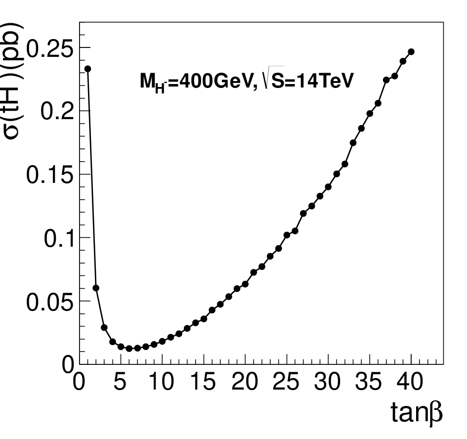
In this section we preform a detailed collider simulation of the pair production and the dominant SM backgrounds. Figure 6 shows the cross section of the scattering as a function of . After exploring the potential of observing the signal events at the 14 TeV LHC with an integrated luminosity of , we examine the top quark polarization measurements and comment on the possibility of determining in the long run.
Since we are interested in the polarization of the top quark or antitop quark from the charged Higgs boson decay, both and processes contribute to the signal events as they both lead to ( denotes the -tagged jet which originates from either a or quark). In reality one cannot tell a -jet and a jet apart. In order to measure the top quark polarization, we demand and use the angle distribution of to measure the top quark polarization. We further require to increase the signal rate. 22 2 The leptonic decay can also be used to determine the top quark polarization. The two missing neutrinos can be fully reconstructed from the missing energy and the on-shell conditions of the bosons and quarks [16, 17]. It then yields an event topology of plus missing energy as follows:
| (24) |

Figure 7 displays the Feynman diagrams of both signal processes with subsequent decays. At the LHC the and initial states give rise to the same production rate. Only half of quarks in the signal event sample are from the decay, and their polarization is completely determined by the chirality structure of the coupling. The other half of quarks emerge at the production level, whose polarization is highly diluted. In order to reveal the connection between the top quark polarization and , one has to find a set of optimal cuts to separate the and signal events.
Two SM backgrounds are considered in this work:
| (25) |
The background is irreducible as it contributes exactly the same event topology as the signal. On the other hand, the reducible background could mimic the signal when the light jet (denoting the light-flavor quarks or gluons) is misidentified as a jet.
III.1 Event selection
In this work we adapt MadGraph/MadEvent [18] to generate both the signal and background processes. The following basic cuts are applied while generating events in MadGraph5,
| (26) |
where denotes the transverse momentum, is the missing transverse momentum from the invisible neutrino in the final state, and is the separation in the azimuthal angle () pseudorapidity () plane between the objects and
| (27) |
Table 1 displays the number of events for the signals and backgrounds at the 14 TeV LHC with an integrated luminosity of for and three values of . The dominant SM background is from the production which is about 3 or 4 orders of magnitude larger than the signal; see the third row in the table. A series of kinematic cuts is needed to extract the small signal out of the tremendous backgrounds. We optimize the cut criteria specially for where the signal is difficult to detect.
| 1 | 6 | 40 | SM backgrounds | |||||
| Inclusive rate | 23310 | 23300 | 1255 | 1227 | 24660 | 23520 | 234000 | |
| Hard cuts | 11843 | 13466 | 687 | 719 | 14421 | 13890 | 25052 | |
| 4980 | 368 | 672 | 20 | 5680 | 383 | 39238 | 386 | |
| 3910 | 305 | 532 | 16 | 4375 | 310 | 14942 | 171 | |
| tagging | 2346 | 183 | 312 | 10 | 2625 | 186 | 299 | 102 |
| Number of events | 2529 | 322 | 2811 | 401 | ||||
| 6.3 | 0.8 | 7.0 | ||||||
| 126.3 | 16.1 | 140.3 | ||||||
| 54.1 | 26.9 | 56.7 | ||||||
III.2 Hard cut on jets
Our signal events consist of five jets in the final sate. As they originate from a heavy scalar decay, the top quark and bottom quark are boosted such that they have a hard . As a result, the jets from the energetic top quark are also highly boosted to yield a hard . On the contrary, the top quarks in the SM backgrounds are predominantly produced in the threshold region where the top quarks are not highly boosted. The jets from top quark decays in the backgrounds tend to be soft. We examine the ’s of the final state jets and impose hard cuts on their ’s to suppress the SM backgrounds.
We order the five jets in the final state by their values in each event:
| (28) |

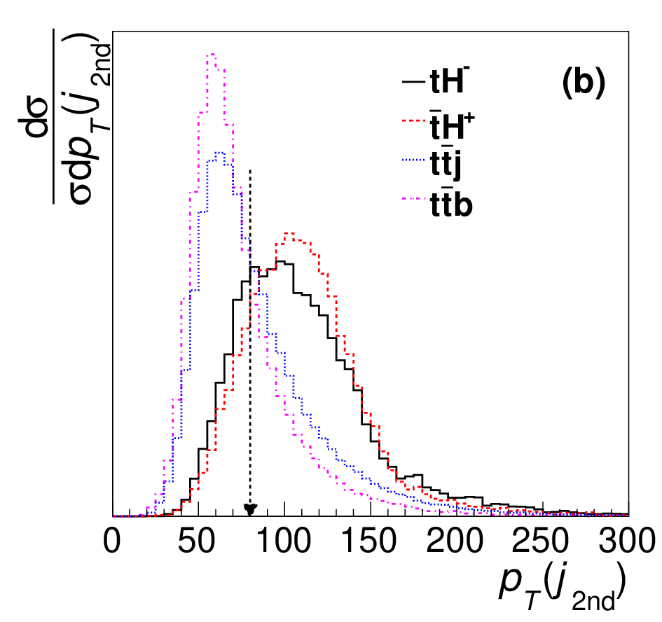
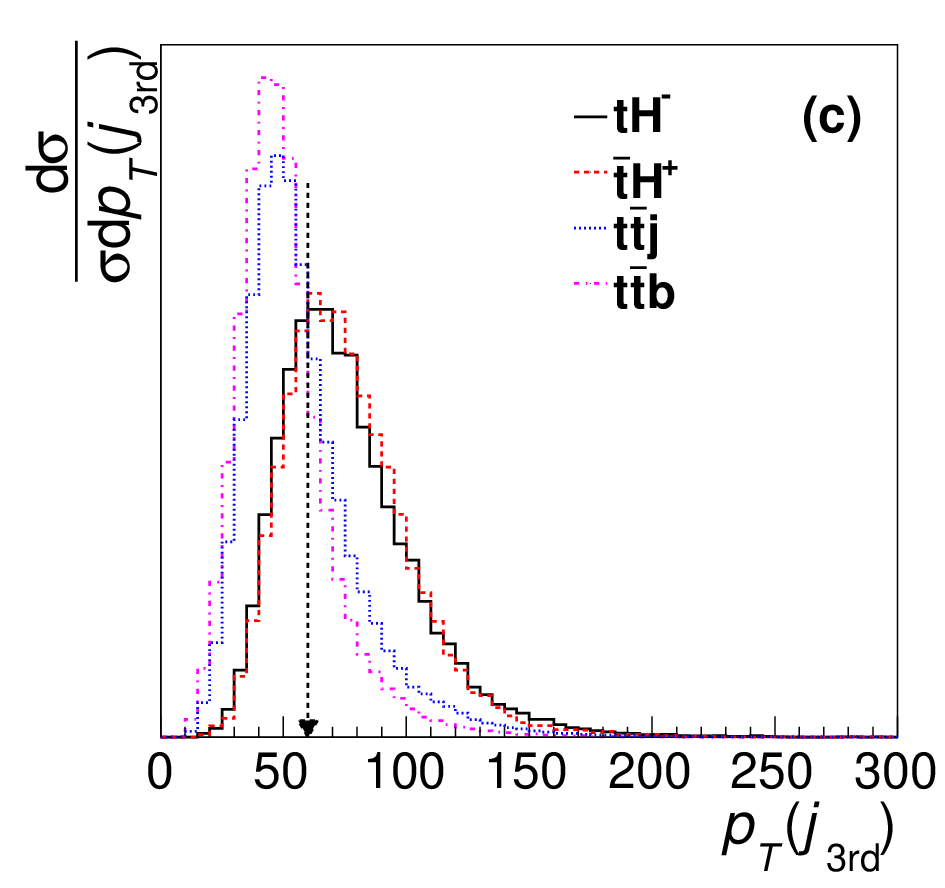
Figure 8 displays the normalized distributions of the ordered jets: (a) the leading (first) jet; (b) the second jet; (c) the third jet. It clearly shows that the signal events exhibit much harder distributions than the SM background events. It enables us to impose hard cuts on the first three hard jets to suppress the SM backgrounds. In this study we adapt a set of hard cuts as follows:
| (29) |
see the vertical dashed-line arrows in Fig. 8. For example, the leading jet is very often the or jet from the charged Higgs boson decay such that its distribution peaks around ; see the solid black and dashed red curves in Fig. 8(a). On the other hand, the leading jet in the background is often the jet from top quark decay and naturally exhibits a peak around in the distribution; see the dotted blue and dashed-dotted magenta curves.
The fourth row in Table 1 shows the number of events after the hard cuts for both signals and backgrounds. The hard cuts remove almost half of the signal events, but they suppress the backgrounds by almost an order of magnitude. At this stage of analysis, the and backgrounds still dominate over the signal processes after the hard cuts given in Eq. (29). The backgrounds are about 80 times larger than the signals for small and large ( or ). For the ratio of the background and signal is about 1500.
III.3 Top reconstruction, mass-window cut and extra-jet tagging
So far we treat all the jets equally and no tagging is performed. The key to suppress the background is to identify the extra jet (denoted as , the jet produced in association with the pair) as a jet. The minimal -template method [19] is adapted to reconstruct the pair and singles out the extra jet.
The minimal -template method is based on the -boson and top quark masses to select the extra jet. For each event we loop over all jet combinations and pick the combination which minimizes the following :
| (30) |
Note that the invisible neutrino needs to be fully determined in order to reconstruct in above equation. The transverse momentum of the neutrino can be determined from the momentum imbalance in the transverse plane while the longitudinal momentum of the neutrino () can be derived from the -boson on-mass-shell condition, . It yields a twofold solution as
| (31) |
when . The ambiguity of the twofold solution is removed also by the minimal requirement. The method is very efficient at identifying the extra jet and reconstructing the leptonically decayed top quark, but it is less efficient at reconstructing the hadronically decayed top quark because of the combinatorial ambiguities of jets in the final state [19].

With a reconstructed quark and quark in hand, we are ready to reconstruct . Figure 9 shows the normalized invariant mass distribution of the and pair, denoted as . Since our signal events consist of both and , one half of the signal events have a sharp peak in the distribution (solid black curve) when the and pair indeed comes from the decay. The pin shape reflects the narrow width of the charged Higgs boson. On the contrary, the other half of the signal events exhibit a fairly broad bump (dashed red curve) as is not from the decay in the process. Similarly, the two SM backgrounds also show a broad spectrum and peak in the low mass region. To further improve the signal-to-background ratio, we require the invariant mass of the reconstructed quark and the extra jet to be within the mass window,
| (32) |
where is the expected experimental resolution for a 400 GeV decaying into a pair. As shown in Table 1, both the and backgrounds are reduced by a factor of around 60 at the cost of the reduction rate in signal by . That increases the signal-to-background ratio by a factor of . The reduction of the signal is mainly from the process which exhibits a continuous nonresonance spectrum of the invariant mass; see the dashed red curve in Fig. 9. Such a nonresonance feature is simply because the and the extra jet are not from the decay. Note that, when , the mass-window cut does not have much impact on the signal process because the boson width is very narrow such that almost all the signal events fall inside the mass window.
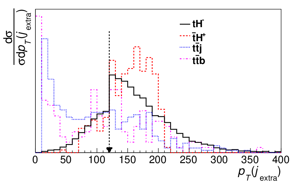
The extra jet in the signal often originates from the heavy decay and tends to have a large . The extra jet in the SM background, predominately from QCD radiation, tends to have a much softer . In Fig. 10 we plot the normalized distribution of the extra jet. It is clear that both (solid black) and (dashed red) signal processes have a large while the background processes peak in the small but still have a long tail in the large region. We impose the following cut on to optimize the signal:
| (33) |
The cut suppresses the background rate by a factor of 3 and keeps about of the signal events; see the sixth row in Table 1.
Finally, we demand that the extra jet be a jet and choose the tagging efficiency as and a moderate mistagging efficiency as [20]. The very last requirement sufficiently eliminates the SM backgrounds; see the seventh row in Table 1. At the bottom of the table we also show the number of both signal and background events after applying all the cuts, the signal-to-background ratio, the statistical significance of the signal, and the statistical uncertainties in the measured signal event rate. It is very promising to observe the signal events after the optimal cuts. The significance of the signal is well above for a broad range of . For , more than 300 signal events survive, which could be used to probe top quark polarization.
IV top quark polarization and measurement
Armed with the reconstructed , and , we are ready to measure -quark polarization. In the helicity basis, the -quark polarization can be found from the distribution in , the angle of the charged lepton in the rest frame of quark relative to the top quark direction of motion in the rest frame of . The angular correlation of is given by
| (34) |
where the () choice is for a left-handed quark while () is for a right-handed quark. The angular distribution of in the rest frame of a quark is the same but with the () choice for the right-handed quark while () is for the left-handed quark. Note that the above formula is insensitive to the next-to-leading order (NLO) QCD corrections, which are only at [21]. The tree-level analysis based on top polarization will not be altered too much even including NLO QCD corrections.
In Fig. 11(a), we plot the normalized distribution of of the signal and background processes with basic cuts in Eq. (26). For the signal processes we choose and . The signal events exhibit a clear shape of . On the contrary, the distribution of the signal is flat, owing to the effects of higher partial waves generated by the -channel diagram. Both the and backgrounds also show a flat distribution. The top quark polarization possessed by the signal is diluted by the signal and the other two SM backgrounds.
In order to demonstrate the dependence of top quark polarization on in the signal events, we plot the normalized distribution of of the channel for and three values of in Fig. 11(b): (solid), (dashed), and (dotted). The top quark is highly polarized for and but is nearly unpolarized for . The results remain the same even after all cuts.


The degree of top quark polarization can be written as the ratio
| (35) |
where () is the number of right-handed (left-handed) polarized top quarks in the helicity basis; for the antitop quark case () is the number of left-handed (right-handed) polarized antitop quarks. Correspondingly the angle distribution of could be written as
| (36) |
Simple algebra leads to the following identity:
| (37) |
We obtain the degree of top quark polarization from the distribution, which is divided into 10 bins:
| (38) |
where is the middle point value of each bin, is the normalized value for each bin, is the bin width and is the number of events falling into each bin. We consider the statistical error for as ; the statistical error for the degree of top quark polarization is calculated as
| (39) |
Based on the degree of polarization we can easily get the spin fraction ,
| (40) |
the fraction of top quarks with spin along the basis direction. We can also define the asymmetry of the distribution of as
| (41) |
where
| (42) |
It is easy to check that without imposing any kinematic cut , but the relation would break down after the kinematic cut. Table 2 displays the degree of polarization , polarization fraction , and asymmetry before cuts and after selection cuts and event reconstruction. From the table we can see that for the top quark is highly polarized, the kinematic cuts change the degree of polarization by ; the relation of still holds.
| No cut | After cut | No cut | After cut | No cut | After cut | ||
| 1 | 0.97 | 0.87 | 0.99 | 0.93 | 0.98 | 0.88 | |
| 0.45 | 0.29 | ||||||
| 6 | 0.12 | 0.56 | 0.46 | 0.10 | |||
| 0.50 | 0.49 | 0.00 | |||||
| 40 | 0.06 | ||||||
| 0.10 | 0.55 | 0.49 | 0.09 | ||||
| 0.06 | 0.09 | 0.53 | 0.55 | 0.03 | 0.04 | ||
| 0.03 | 0.43 | 0.51 | 0.25 | ||||
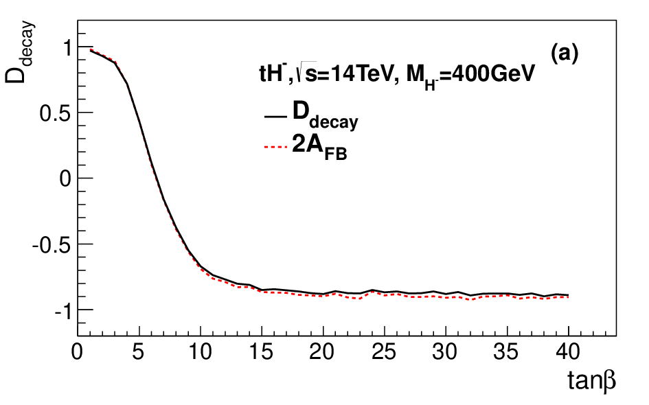
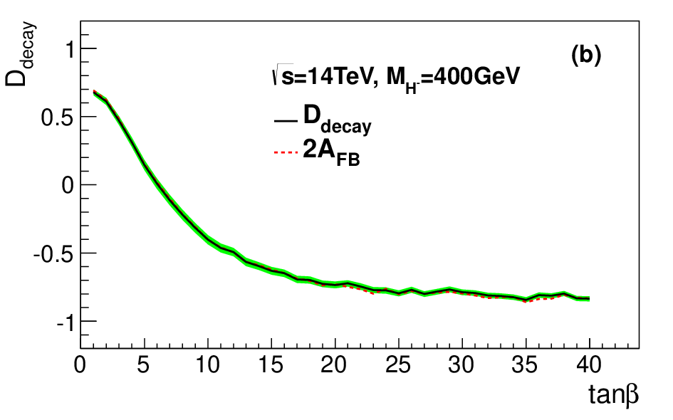
Figure 12(a) shows the degree of polarization of the antitop quark as a function of in the signal process for . The is also plotted for comparison. The top quark polarization is a good probe for a wide range of . The intermediate has been considered very hard to measure. Figure 12 shows that the varies rapidly in the region of . This feature enables us to determine using top polarization. However, the degree of polarization cannot be used to determine the value of in the large region as the degree of polarization approaches -1. Including the signal and the two SM backgrounds inevitably reduces the degree of polarization, as depicted in Fig. 12(b). The green band [cf. Eq. (39)] shows the statistical uncertainties derived from all the signal and background events after all the kinematic cuts and event reconstructions.
V Conclusion and Discussion
The charged Higgs boson, an undoubted signal of new physics, appears in many new physics models. In the type-II two-Higgs-doublet model the chirality structure of the coupling of charged Higgs boson to the top and bottom quarks is very sensitive to the value of . As the polarization of the top quark can be measured experimentally from the top quark decay products, one could make use of the top quark polarization to determine the value of . In this work we preform a detailed analysis of measuring top quark polarization in the charged Higgs boson production channels and . We calculate the helicity amplitudes of the charged Higgs boson production and decay. Our calculation shows that the top quark from the charged Higgs boson decay provides a good probe for measuring , especially for the intermediate region. On the contrary, the top quark produced in association with the charged Higgs boson cannot be used to measure because its polarization is highly contaminated by the -channel kinematics.
The analysis in this paper is based on tree-level estimation for signal and background, and we would like to comment on the higher-order effects. The NLO QCD corrections to the process have been calculated in Ref. [14]. It is shown that the ratio of the NLO cross section to the LO cross section varies roughly from to when the charged Higgs boson mass increases from 200 to 1000 GeV. The NLO QCD corrections can reduce the scale dependence of the LO cross section. In order to simulate the real collider environment, one needs to use a full parton shower, including both the initial state radiation (ISR) and the final state radiation (FSR), to calculate more precisely the physical observables, e.g., the jet multiplicity, jet transverse momentum and energy, etc. Our signal events consist of five jets from heavy resonance decays such that the jets exhibit a large transverse momentum; see Fig. 8. On the other hand, the ISR and FSR tend to produce soft jets, which are not often able to pass the stringent cuts imposed on the of jets in our analysis. Our results should not vary dramatically by the ISR and FSR effects. Needless to say, it is necessary to perform a thorough analysis including the parton shower effects to get a more realistic prediction on the signal discovery potential, top quark reconstruction efficiency, the uncertainty of measuring top quark polarization, etc. But it is beyond the scope of the current paper and should be presented elsewhere.
Acknowledgements.
We thank Chen Zhang for checking helicity amplitudes and many useful discussions. Q.H.C. is supported in part by the National Science Foundation of China under Grant No. 11245003. The work of X.W., X.P.W. and S.H.Z. was supported in part by the Natural Science Foundation of China under Grants No. 11075003 and No. 11135003. X.W. is also supported in part by the China Postdoctoral Science Foundation under Grant No. 2012M520098.References
- [1] G. Branco et al., Phys.Rept. 516, 1 (2012), arXiv:1106.0034.
- [2] C.-s. Huang and S.-H. Zhu, Phys. Rev. D61, 015011 (2000), arXiv:hep-ph/9905463.
- [3] C.-S. Huang, W. Liao, Q.-S. Yan, and S.-H. Zhu, Eur. Phys. J. C25, 103 (2002), arXiv:hep-ph/0110147.
- [4] K. Huitu, S. Kumar Rai, K. Rao, S. D. Rindani, and P. Sharma, JHEP 1104, 026 (2011), arXiv:1012.0527.
- [5] R. M. Godbole, L. Hartgring, I. Niessen, and C. D. White, JHEP 1201, 011 (2012), arXiv:1111.0759.
- [6] X. Gong, Z.-G. Si, S. Yang, and Y.-j. Zheng, Phys.Rev. D87, 035014 (2013), arXiv:1210.7822.
- [7] J. Baglio et al., Phys.Lett. B705, 212 (2011), arXiv:1109.2420.
- [8] D. Eriksson, G. Ingelman, J. Rathsman, and O. Stal, JHEP 0801, 024 (2008), arXiv:0710.5906.
- [9] O. Deschamps et al., Phys.Rev. D82, 073012 (2010), arXiv:0907.5135.
- [10] R. M. Barnett, H. E. Haber, and D. E. Soper, Nucl.Phys. B306, 697 (1988).
- [11] F. I. Olness and W.-K. Tung, Nucl.Phys. B308, 813 (1988).
- [12] C. S. Huang and S.-H. Zhu, Phys. Rev. D60, 075012 (1999), arXiv:hep-ph/9812201.
- [13] F. Borzumati, J.-L. Kneur, and N. Polonsky, Phys.Rev. D60, 115011 (1999), arXiv:hep-ph/9905443.
- [14] S.-h. Zhu, Phys. Rev. D67, 075006 (2003), arXiv:hep-ph/0112109.
- [15] T. Plehn, Phys.Rev. D67, 014018 (2003), arXiv:hep-ph/0206121.
- [16] E. L. Berger, Q.-H. Cao, C.-R. Chen, G. Shaughnessy, and H. Zhang, Phys. Rev. Lett. 105, 181802 (2010), arXiv:1005.2622.
- [17] H. Zhang, E. L. Berger, Q.-H. Cao, C.-R. Chen, and G. Shaughnessy, Phys. Lett. B696, 68 (2011), arXiv:1009.5379.
- [18] J. Alwall, M. Herquet, F. Maltoni, O. Mattelaer, and T. Stelzer, JHEP 1106, 128 (2011), arXiv:1106.0522.
- [19] E. L. Berger, Q.-H. Cao, J.-H. Yu, and C.-P. Yuan, Phys. Rev. D84, 095026 (2011), arXiv:1108.3613.
- [20] ATLAS Collaboration, G. Aad et al., (2009), arXiv:0901.0512.
- [21] A. Czarnecki, M. Jezabek, and J. H. Kuhn, Nucl. Phys. B351, 70 (1991).