On the precoder design of a wireless energy harvesting node in linear vector Gaussian channels with arbitrary input distributionThanks: This work was partially supported by: the Catalan Government under grants 2009SGR 1046 and 2011FI_B 00956; the Spanish Ministry of Economy and Competitiveness under project TEC2011-29006-C03-01 (GRE3N-PHY); and the European Commission in the framework of the FP7 Network of Excellence in Wireless COMmunications NEWCOM# (Grant agreement no. 318306).
Abstract
A WEHN (WEHN) operating in linear vector Gaussian channels with arbitrarily distributed input symbols is considered in this paper. The precoding strategy that maximizes the mutual information along independent channel accesses is studied under non-causal knowledge of the channel state and harvested energy (commonly known as offline approach). It is shown that, at each channel use, the left singular vectors of the precoder are equal to the eigenvectors of the Gram channel matrix. Additionally, an expression that relates the optimal singular values of the precoder with the energy harvesting profile through the MMSE (MMSE) matrix is obtained. Then, the specific situation in which the right singular vectors of the precoder are set to the identity matrix is considered. In this scenario, the optimal offline power allocation, named Mercury Water-Flowing, is derived and an intuitive graphical representation is presented. Two optimal offline algorithms to compute the Mercury Water-Flowing solution are proposed and an exhaustive study of their computational complexity is performed. Moreover, an online algorithm is designed, which only uses causal knowledge of the harvested energy and channel state. Finally, the achieved mutual information is evaluated through simulation.
Index Terms:
Energy harvesting, mutual information, arbitrary input distribution, precoder optimization, power allocation, linear vector Gaussian channels, MMSE.I Introduction
Battery powered devices are becoming broadly used due to the high mobility and flexibility provided to users. As Moore predicted in 1965 [1], nodes’ processing capability keeps increasing as transistors shrink year after year. However, the growth of battery capacity is slower and thus energy availability is becoming the bottleneck in the computational capabilities of wireless nodes.
Energy harvesting, which is known as the process of collecting energy from the environment by different means (e.g. solar cells, piezoelectric generators, etc.), has become a potential technology to charge batteries and, therefore, expand the lifetime of battery powered devices (e.g., handheld devices or sensor nodes), which we refer to as WEHN. The presence of energy harvesters implies a loss of optimality of the traditional transmission policies, such as the well-known WF (WF) strategy [2], because the common transmission power constraint must be replaced by a set of ECC, which impose that energy must be harvested before it can be used by the node.
In general, the energy harvesting process is modeled as a set of energy packets arriving to the node at different time instants and with different amounts of energy.11 1 Observe that any energy harvesting profile can be accurately modeled by making the inter arrival times sufficiently small. There exist two well established approaches for the design of optimal transmission strategies, namely, online and offline. The online approach assumes that the node only has some statistical knowledge of the dynamics of the energy harvesting process, which can be realistic in practice. The offline approach assumes that the node has full knowledge of the amount and arrival time of each energy packet, which is an idealistic situation that provides analytical and intuitive solutions and, therefore, it is a good first step to gain insight for the later design of the online transmission strategy. Using this model for the energy harvesting process, references [3, 4, 5, 6, 7, 8, 9, 10] derived the optimal resource allocation in different scenarios. The authors of [6] and [7] found the power allocation strategy, named DWF (DWF), that maximizes the total throughput of a WEHN operating in a point-to-point link, i.e.,
| (1) |
where is the channel use index, is the channel gain, is a set that contains the channel accesses between two consecutive energy arrivals, and is the water level associated to .22 2 Notation: Matrices and vectors are denoted by upper and lower case bold letters, respectively. denotes the -th component of the vector . is the component in the -th row and -th column of matrix . is the identity matrix of order , is a column vector of ones. denotes the Jacobian of the matrix function w.r.t. (w.r.t.) the matrix variable [11]. The superscript denotes the transpose operator. is the column vector that contains the diagonal elements of the matrix . is a diagonal matrix where the entries of the diagonal are given by the vector . returns a vector that stacks the columns of . denotes the trace of a matrix. is the variance of some random variable. The Kronecker product is denoted by the symbol . Finally, .
For nodes without energy harvesting capabilities, the capacity of linear vector Gaussian channels was given in [12], where it was shown that given a certain constraint in the transmitted power, , capacity is achieved by diagonalizing the observed channel in independent streams. Then, a Gaussian distributed codeword is transmitted over each stream whose power is obtained from the well known WF solution:
| (2) |
The main difference between DWF (1) and WF (2) is that in the former the water level depends on the channel access under consideration.
Both (1) and (2) are optimal when the distribution of the input is Gaussian. However, in practical scenarios, finite constellations are used instead of the ideal Gaussian signaling, e.g., -PAM and -QAM, where denotes the alphabet cardinality. In the low SNR (SNR) regime, the capacity achieved with finite constellations is very close to the one achieved by Gaussian signaling. However, the mutual information asymptotically saturates when the SNR increases as not more than bit per channel use can be sent (see Fig. 1 in [13]). This must be taken into account in the design of the optimal power allocation when the input symbols are constrained to belong to a finite alphabet. In opposition to the Gaussian case, where the better the channel gain, the higher the allocated power, when arbitrary constellations are used, there exists a tradeoff between the alphabet cardinality and the channel gain. In [14], the optimal power allocation was found for a node without energy harvesting capabilities and with arbitrary distributed input symbols. To do so, the authors of [14] used the relation between the mutual information and the MMSE, which was revealed in [15] and further generalized in [16], as summarized in the following lines.
In [15], Guo et al. revealed that the derivative of the mutual information with respect to (w.r.t.) the SNR for a real-valued scalar Gaussian channel is proportional to the MMSE, i.e.,
| (3) |
where is the channel input, is the observed noise and , where is the conditional mean estimator. The mutual information in linear vector Gaussian channels was further characterized in [16], where its partial derivatives w.r.t. arbitrary system parameters were determined, e.g., the gradient w.r.t. the channel matrix, , was found to be
| (4) |
where is the vector input, is the noise, is the MMSE matrix, and .
Thanks to the relationship in (3), the power allocation that maximizes the mutual information over a set of parallel channels (each of them denoted by a different index ) with finite alphabet inputs was derived in [14] and named Mercury/Waterfilling (WF), i.e.,
| (5) |
where is the mercury factor that depends on the input distribution and is defined as
| (6) |
This result showed that the optimal power allocation not only depends on the channel gain as in the Gaussian signaling case, but also on the shape and size of the constellation.
The goal of this work is to design the transmitter that maximizes the mutual information along channel uses by jointly considering the nature of the energy harvesting process at the transmitter and arbitrary distributions of the input symbols, which, to the best of our knowledge, has not been yet considered in the literature. Hence, the main contributions of this paper are: (i.) Proving that, at the -th channel use, the left singular vectors of the -th precoder matrix are equal to the eigenvectors of the -th channel Gram matrix. (ii.) Deriving an expression that relates the singular values of the -th precoder matrix with the energy harvesting profile through the MMSE matrix. (iii.) Showing that the derivation of the optimal right singular vectors is a difficult problem and proposing a possible research direction towards the design of a numerical algorithm that computes the optimal right singular vectors. The design of this numerical algorithm is out of the scope of the current paper because our focus is to gain insight from the closed form power allocation that is obtained after setting the right singular vectors matrix to be the identity matrix and, in this scenario, the contributions are: (iv.) Deriving the optimal offline power allocation, named the Mercury Water-Flowing solution, and providing an intuitive graphical interpretation, which follows from demonstrating that the mercury level is monotonically increasing with the water level. (v.) Proposing two different algorithms to compute the Mercury Water-Flowing solution, proving their optimality, and carrying out an exhaustive study of their computational complexity. (vi.) Implementing an online algorithm, which does not require future knowledge of neither the channel state nor the energy arrivals, that computes a power allocation that performs close to the offline optimal Mercury Water-Flowing solution.
The remainder of the paper is structured as follows. Section II presents the system model. In Section III, the aforementioned problem is formally formulated and solved. The graphical interpretation of the Mercury Water-Flowing solution is given in Section IV. The offline and online algorithms are introduced in Sections V and VI, respectively. In Section VII, the performance of our solution is compared with different suboptimal strategies and the computational complexity of the algorithms is experimentally evaluated. Finally, the paper is concluded in Section VIII.
II System model
We consider a point-to-point communication through a discrete-time linear vector Gaussian channel where the transmitter is equipped with energy harvesters. A total of channel uses are considered where at each channel use the symbol is transmitted.33 3 The real field has been considered for the sake of simplicity. The extension to the complex case is feasible but requires the definition of the complex derivative, the generalization of the chain rule, and cumbersome mathematical derivations, which is out of the scope of this work. Nevertheless, the extension to the complex case can be done similarly as [17] generalized the results obtained in [18].
We consider that the symbols have independent components with unit power, i.e., and that they are i.i.d. (i.i.d.) along channel uses according to . As shown in Fig. 1, the symbol is linearly processed at the transmitter by the precoder matrix . We consider a slow-fading channel where the coherence time of the channel is much larger than the symbol duration , i.e., . Thus, a constant channel matrix is considered at the -th channel use. Let denote the rank of the channel matrix, i.e., , then we have that .44 4 We have considered that is not rank deficient, , which is a realistic assumption due to random nature of the channel. Thus, the received signal at the -th channel use is
| (7) |
where represents the zero-mean Gaussian noise with identity covariance matrix .55 5 Note that if the noise is colored and its covariance matrix is known, we can consider the whitened received signal . Let denote the -th channel use MMSE matrix, which is defined as and is the conditional mean estimator.
Let us express the channel matrix as , where is a diagonal matrix that contains the largest eigenvalues of and and are semi-unitary matrices that contain the row and column associated eigenvectors, respectively. The precoder matrix can be expressed as , where , is a diagonal matrix whose entries are given by the vector and is a unitary matrix. Full CSI (CSI) is assumed at the transmitter.

The energy harvesting process at the transmitter is characterized by a packetized model, i.e., the node is able to collect a packet of energy containing Joules at the beginning of the channel access. Let be the total number of packets harvested during the channel uses. The initial battery of the node is modeled as the first harvested packet at . We assume that the mean time between energy arrivals, , is considerably larger than the symbol duration time, i.e., and thus we can consider that packet arrival times are aligned at the beginning of a channel use.66 6 In our model, the transmitter can only change its transmission strategy in a channel access basis. Accordingly, if an energy packet arrives in the middle of a channel access, we can assume that the packet becomes available for the transmitter at the beginning of the following channel access. First, in Sections III-V, we consider the offline approach as it provides analytical and intuitive expressions. Afterwards, in Section VI, we develop an online transmission strategy where the transmitter only has causal knowledge of the energy harvesting process, i.e., about the past and present energy arrivals. We use the term pool, , to denote the set of channel accesses between two consecutive energy arrivals. As in [3] and [8], we assume an infinite capacity battery since, in general, the battery size is large enough so that the difference between the accumulated harvested energy and the accumulated expended energy is always smaller than the battery capacity. A temporal representation is given in Fig. 2.

III Throughput maximization problem
In this section, we study the set of linear precoding matrices that maximizes the input-output mutual information along independent channel accesses, , where is the -th channel use mutual information. The design of is constrained to satisfy instantaneous ECC, which impose that energy cannot be used before it has been harvested, , . However, since in each pool there are several channel accesses with the same channel gains (because and ), instead of imposing the instantaneous ECC, we can consider the mean ECC that become , , which do not require prior knowledge of the transmitted symbols at each channel use as only the expectation of the symbols is needed.77 7 In general, the energy harvesting and the channel state are two independent random processes, thus, there may be situations in which only a few a few channel accesses separate an energy arrival from a change of the channel realization, however, note that these situations are unlikely since and . In these improbable situations, the temporal averaging is not sufficient to ensure that the fulfillment of the mean ECC implies a fulfillment of the instantaneous ECC, however, the averaging through the different channel dimensions brings closer the mean and instantaneous ECC. Thus, the mean ECC can be used instead of the instantaneous ECC since the cases in which they differ are indeed very unlikely.
Therefore, the mutual information maximization is mathematically expressed as
| (8a) | |||||
| (8b) | |||||
Before addressing the problem in (8), let us summarize the state of the art on the precoding strategy that maximizes the mutual information for non-harvesting nodes, which was studied in [19, 18, 20, 17] and references therein.88 8 When there is no energy harvesting in the transmitter, the mutual information maximization problem is the one obtained after setting and in (8). Thus, the mutual information is maximized for a single channel use under a power constraint. In [19], it was shown that, in general, the mutual information, , is not a concave function of the precoder and that depends on the precoder only through the matrix . The authors of [19] also showed that the left singular vectors of the precoder can be chosen to be equal to the eigenvectors of the channel Gram matrix, i.e., . From this, and the mutual information depends on the precoder only through the right eigenvectors and the associated singular values. In [18], it was shown that is a concave function of the squared singular values of the precoder, , when a diagonal channel matrix is considered. Finally, the authors of [19] stated that the complexity in the design of the globally optimal precoder lies in the right singular vectors of the precoder, . Then, in [20], it was shown that is a concave function of the matrix and a gradient algorithm over was derived to find a locally optimal precoder. References [19, 18, 20] considered a real channel model. The extension to the complex case was done in [17], where the authors pointed out that by allowing the precoder and the channel matrix to be in the complex field the mutual information can be further improved. Then, they proposed an iterative algorithm that determines the globally optimal precoder that imposes that the power constraint must be met with equality.
When energy harvesting is considered, instead of having a single power constraint, we have a set of ECC as in (8b) and it is not straightforward to determine which of the constraints must be met with equality. This fact implies that the algorithm introduced in [17] is no longer optimal when energy harvesting is considered. Altogether, (8) is not a convex optimization problem since the mutual information is not a concave function of the precoder and, hence, its solution is not straightforward. In the following lemma, we generalize Proposition 1 in [19] for the case of considering energy harvesting in the transmitter.
Lemma 1.
The left singular vectors of the -th precoder matrix, , are equal to the eigenvectors of the channel Gram matrix , .
Proof:
See Appendix A. ∎
Thanks to Lemma 1, the optimal precoding matrix is , and the dependence of on the precoder is only through and . In the following lines, we maximize the mutual information w.r.t. for a given . By applying Lemma 1 in (7), the next equivalent signal model is obtained
| (9) |
where and is deterministic and known. To fully exploit the diversity of the channel, we assign the dimension of the input vector to be equal to the number of channel eigenmodes, i.e., . It is easy to verify that the maximization of the mutual information w.r.t. is not a convex optimization problem. However, if instead we maximize the mutual information w.r.t. the squared singular values of the precoder , the obtained problem is convex, as shown in the following lines. Thus, the problem reduces to
| (10a) | |||||
| (10b) | |||||
Observe that, at the -th channel access, the input-output mutual information is concave w.r.t. , which was proved in [18]. Therefore, the objective function is concave as the sum of concave functions is concave [21]. Finally, as the constraints are affine in , (10) is a convex optimization problem and the KKT are sufficient and necessary optimality conditions. In particular, the optimal solution must satisfy (the reader who is not familiar with this notation, which is presented in [11], is referred to [18, Appendix B] for a concise summary), where is the Lagrangian that is , where are the Lagrange multipliers associated with the inequality constraints. We want to remark that in all the expressions derived in the remainder of the paper, refers to some channel access contained in , which follows from the formulation of . In order to obtain , we first need to determine the Jacobian matrix of the mutual information w.r.t. , which is done in the following lemma:
Lemma 2.
The Jacobian matrix of the mutual information w.r.t. is .
Proof:
See Appendix B. ∎
With this result, we can proceed to solve the KKT condition :
| (11) |
where is the -th pool water level, i.e.,
| (12) |
From (11), at each channel use, we obtain a set of conditions that relate the power allocation in each stream (through the MMSE matrix) with the energy harvesting profile (through the pool’s water level). Some properties of the water level can be derived from the KKT optimality conditions:
| (13) | |||||
| (14) |
Plugging (13) in (12), it is straightforward to obtain the following property:
Property 1.
The water level is non-decreasing in time.99 9 This property is only valid under an infinity battery capacity assumption. When a finite battery is considered the water level may increase or decrease [7].
From (14), we can get more insights in the solution. There are two possibilities to fulfill (14):
- •
Empty Battery: This situation occurs when, at the end of the -th pool, the node has consumed all the energy, i.e., .
- •
Energy Flow: This situation occurs when, at the end of the -th pool, the node has some remaining energy in the battery, which will be used in the following pools. When this happens and, hence, .
Property 2.
Changes on the water level are only produced when at the end of the previous pool the node has consumed all the available energy.
Note that the ECC take into account the energy spent by the node over all the dimensions. Thus, these two properties also hold in a scalar channel model as proved in [6, Theorem 3].
Since the problem in (10) is convex, by using (11) and Properties 1 and 2, we can construct efficient numerical algorithms to compute the optimal power allocation, , for a given . The maximization of the mutual information w.r.t. is indeed much more complicated as pointed out in [19] for the non-harvesting scenario. In this context, in this work, we focus on the particular case in which because, in spite of not being necessarily the globally optimal precoder, it leads to an analytical closed form power allocation that allows an intuitive graphical representation of the solution, as it is explained in the next section. Observe that for any other choice , we must resort to numerical methods to compute the optimal power allocation.
The design and development of a numerical algorithm that computed the globally optimal precoder at each channel access would be an interesting research problem in its own and is left for future research. We believe that a possible starting point would be to analyze how to expand the algorithms presented in [20] and [17], which exploit the concavity of the mutual information w.r.t. the matrix and the fact that the power constraint must be met with equality, to the energy harvesting scenario. Note that if we knew the optimal total power allocation in each channel access, we could run times the algorithm proposed in [20] to obtain the globally optimal precoder in each channel access, however, this approach has two major drawbacks. First, the optimal total power allocation in each channel access is not known a priori and its computation is not straightforward since the total power consumptions of the different channel accesses belonging to the same pool must simultaneously satisfy (11). The second drawback is the required computational burden since any iterative approach requires a new estimation of the MMSE matrix, , at every iteration since it depends on and . These two reasons makes challenging the applicability of the proposed approach and, hence, different alternatives to find the globally optimal precoder may be required. Altogether, we believe that the development of a numerical algorithm that computes the globally optimal precoder for a WEHN is the object of a new paper in its own and is left for future research.
IV The Mercury Water-Flowing solution
In the remainder of the paper, we consider a communication system in which the precoder is constrained to satisfy or, equivalently, a communication system such that both the precoder and channel matrices are diagonal. In spite of the fact that total achievable mutual information is reduced by forcing , we consider that it is interesting to study this scenario for the following three reasons: (i.) The system , with being the observed noise at the receiver, is commonly encountered in practical systems where, for simplicity at the decoder, independent symbols are transmitted in each dimension (e.g., in multi-tone transmissions like OFDM (OFDM)), and it has been broadly considered in the literature, indeed, the WF solution was derived for such an input-output system model in [14]. (ii.) The optimal power allocation, which is named Mercury Water-Flowing, accepts a closed form expression and an intuitive graphical representation. (iii.) We believe that the intuition gained thanks to the Mercury Water-Flowing graphical interpretation may help for the design of the algorithm that computes the globally optimal precoder of the problem in (8).
In this context, the input-output model can be obtained from the general model in (9) by setting and . From this, we obtain that the equivalent noise is . Thus, a set of independent parallel streams are observed at each channel use. The received signal in the -th stream is where the transmitted symbol is the k-th component of , i.e., , is the observed noise, is the channel gain, and is the transmission radiated power. Therefore, in this section we solve the following optimization problem:
| (15) |
Note that since a linear unitary rotation in the received signal does not affect the input-output mutual information [17]. Thus, the power allocation that maximizes (15) is equal to the one that maximizes (10) and it can be obtained by particularizing (11) with , i.e., . From where, it follows that
| (16) |
where is the inverse MMSE function, defined as in [14], that returns the SNR of the -th stream for a given MMSE, which depends on the probability distribution of .
To present the graphical interpretation of the solution, we need to reformulate (16) as
| (17) |
where is defined in (6) [14], depends on the modulation used, and satisfies the next lemma:
Lemma 3.
The function is monotonically decreasing in .
Proof:
See Appendix C. ∎
Remark 1.
To demonstrate the validity of the graphical representation presented in this section, we need to analytically demonstrate that is monotonically decreasing in . In [14], it was already stated that is decreasing, however, the authors did not provide an analytical proof for their statement. Therefore, we consider that Lemma 3 and its explicit proof are crucial to validate the graphical representation introduced in this section.
Observe the similarity of the power allocation found in (17) with the WF in (5) [14]. The main difference of our solution is that, due to the nature of the energy harvesting process, the water level depends on the channel access. Indeed, from Properties 1 and 2 we have seen that the node is able to increase the water level as energy is being harvested.
Moreover, observe that if we particularize (17) for Gaussian distributed inputs, which have , , (see [14]), the DWF solution in [7] is recovered. Therefore, the mercury factor gives a measure of how power allocation is modified when using non-Gaussian input distributions.
Let be the mercury level of the -th stream at the -th channel use, i.e.,
| (18) |
which depends on the gain and water level of the channel use. Then, the power allocated in a certain stream is the difference between the water and mercury levels, i.e., . The solution interpretation presented in this section is based on the fact that the mercury level is monotonically increasing in , which follows directly from Lemma 3, and generalizes both the WF and the DWF solutions derived in [14] and [7], respectively. The Mercury Water-Flowing interpretation, depicted in Fig. 3, is the following:
- 1.
Each parallel channel is represented with a unit-base water-porous mercury-nonporous vessel1010 10 The vessel boundaries are not depicted in Fig. 3 for the sake of simplicity..
- 2.
Then, each vessel is filled with a solid substance up to a height equal to .
- 3.
A water right-permeable material is used to separate the different pools.
- 4.
Each vessel has a faucet that controls the rhythm at which mercury is poured. The faucet modifies the mercury flow so that the relation between mercury and water levels in (18) is always satisfied.
- 5.
Simultaneously,
- •
The water level is progressively increased to all pools at the same time, adding the necessary amount of water to each pool. The maximum amount of water that can be externally added at some pool is given by the pool’s harvested power (). Let the water freely flow right through the different pools.
- •
Mercury is added to each of the vessels at a different rhythm which is controlled by the vessel’s faucet.
- •
- 6.
The optimal power allocation in each parallel channel is found when all the pools have used all the harvested energy and is obtained as the difference between the water and mercury levels.

V Mercury Water-Flowing offline algorithms
We have designed two different algorithms to compute the optimal Mercury Water-Flowing solution, namely, the NDA (NDA) and the FSA (FSA), which are presented in Sections V-A and V-B, respectively. Afterwards, in Section V-C, we prove the algorithms’ optimality and analyze their computational complexity.
As shown by the KKT optimality conditions, the water in a certain pool may flow to the pools at its right (i.e., from prior to later time instants). This way, the water level over a consecutive set of pools may be equalized. This set of constant water level pools is referred to as an epoch, , where is the total number of epochs and it is unknown a priori. Note that, since the pools are a partition of the epochs, a certain pool is only contained in one epoch. However, an epoch may contain several pools, therefore, .
To compute the power allocation in (17), we just need to determine which pools are contained in each epoch as, once the epochs are known, the optimal power allocation of the epoch can be found by performing the Mercury/Waterfilling Algorithm () introduced in [14], where the -th epoch water level, , is found by forcing that the energy expended in the epoch has to be equal to the energy harvested, which follows from Property 2.
The following two algorithms use a different approach two determine the epochs:
V-A NDA
The NDA uses the fact that a water level decrease is suboptimal, which follows from the KKT conditions (see Property 1), to compute the optimal power allocation as follows:
- 1.
Initially, set , i.e., every epoch contains one pool ,
- 2.
Perform the in [14] to every epoch to obtain the water level, , in each epoch.
- 3.
Look for some epoch, , at which the water level decreases, i.e., :
- •
If some epoch is found, merge this epoch with the following epoch, i.e., . The harvested energy of the resulting epoch is the sum of the two original epochs. Then, the total number of epochs has been reduced by one, i.e., . Perform the to obtain the new water level of the -th epoch, i.e., , and go back to 3.
- •
If no epoch is found, the optimal has been found along with the optimal power allocation.
- •
V-B FSA
The FSA determines the different epochs by finding the optimal transition pools, , that are defined as the first pool of each epoch. As stated before, once the epochs are known the optimal power allocation is determined by applying the to each epoch.1111 11 Observe that, by definition, is the first channel use. To determine , we have designed a forward-search algorithm that extends the algorithm introduced in [6] to take into account arbitrary input distributions. We explain how to obtain and the others are found in the same manner:
- 1.
Assume that the first epoch contains all the pools, .
- 2.
Perform the in [14] to the epoch.
- 3.
The same procedure is repeated to determine the following transition pools until the -th pool is included in some epoch. When this happens, the optimal power allocation has been found for all the channel accesses and streams.
V-C Optimality and performance characterization of the offline algorithms
In this section, first, we demonstrate the optimality of the NDA and the FSA, which is presented in Theorem 1 and, afterwards, we characterize their associated computational complexity.
Proof:
See Appendix D. ∎
With the previous theorem, we have demonstrated that both algorithms compute the optimal power allocation, however, the computational cost of such a computation may be very different. To evaluate this, in Appendix E, we have conducted an exhaustive study on the computational complexity of each of these two algorithms.
Our performance analysis is three-fold, namely, the best, worst, and average computational complexities are computed. Note that both algorithms internally call the a certain number of times to find the optimal solution. Let denote the number of calls to the required to compute the Mercury Water-Flowing solution, which depends on the algorithm itself and on the dynamics of the energy harvesting process. In this context, the best or worst computational complexity is the performance when the minimum or maximum number of calls to are required, respectively. The average computational complexity uses a probabilistic model to compute the average number of calls to . Basically, for the NDA we assume that there is a fixed probability that the water level decreases from epoch to epoch, whereas, for the FSA we assume that there is a fixed probability that a certain ECC is not satisfied. Both and can be experimentally adjusted depending on the energy harvesting profile. The computational complexity in terms of operations (Op.), as well as, in terms of is summarized in Table I, where is a constant parameter that depends, among others, on the size of the MMSE table required to compute the inverse MMSE function and on the tolerance used in the stopping criteria of the . The details of the derivations of the different computational complexities can be found in Appendix E. In Section VII-B, the theoretical results on the algorithms’ computational complexities are compared with the ones obtained through simulation.
VI Online algorithm
Up to now, we have assumed that the transmitter has non-causal knowledge of both the CSI and the energy harvesting process, which is not a realistic assumption in practice. Therefore, the Mercury Water-Flowing solution provides an upper bound on the achievable mutual information of practical schemes in which . In this section, we develop an online algorithm, which is strongly based on the optimal offline solution, the Mercury Water-Flowing power allocation, but that does not require future knowledge of neither the energy arrivals nor the channel state, that computes a suboptimal power allocation of the problem in (15).
Let be the flowing window that is an input parameter of the online algorithm that refers to the number of channel accesses in which the water is allowed to flow, which can be obtained by a previous training under the considered energy harvesting profile, and let an event denote a channel access in which a change in the channel state is produced or an energy packet is harvested, i.e., , , where . In this context, the proposed online algorithm proceeds as follows: (1.) The initial energy in the battery, , is allocated to the different streams of the first channel accesses according to the where the channel is expected to be static and equal to the gain of the first channel use . (2.) When the transmitter detects an event, it updates the allocated power of the channel accesses by using the with the remaining energy in the battery and with the energy of the harvested packet (if the event is an energy arrival), i.e., , and by assuming that the channel remains constant during the flowing window, i.e., , . Note that the transmitter may stay silent in some channel accesses if the difference between two consecutive incoming energy packets is greater than the flowing window, .1212 12 This situation rarely takes place in practice since, in most common situations, is several times the mean number of channel accesses per pool. For example, in the simulated framework presented in Section VII, we have obtained that is 4.4 times the mean number of channel accesses per pool. Step (2.) is repeated until the -th channel access is reached. The proposed online algorithm satisfies ECC and, as pointed out, does not require future information of neither the channel state nor the energy arrivals.
The performance in terms of achieved mutual information depends on the correctness of the estimation of the flowing window, , as discussed with the numerical analysis in Section VII. In summary, this online algorithm provides us a lower bound on the mutual information that can be achieved with sophisticated online algorithms that make use of precise statistical models of the energy harvesting process and channel state.1313 13 A myriad of works have dealt with channel modeling, however, having a precise statistical model of the energy harvesting process is indeed not trivial as it depends on many factors such as the harvester used by the node (e.g., a solar panel, piezoelectric generator, etc.), the node’s placement, mobility, etc.
VII Results
This section first evaluates the gain of the proposed Mercury Water-Flowing solution with respect to other suboptimal solutions and, secondly, it presents an analysis through simulation of the computational complexity of the NDA and FSA.
VII-A Results on Mercury Water-Flowing solution
In this section, we evaluate the mutual informations obtained with the optimal offline solution, the Mercury Water-Flowing (-), and with the online policy presented in Section VI.
To the best of our knowledge, there are no offline algorithms in the literature that maximize the mutual information by jointly considering energy harvesting at the transmitter and arbitrary distributed input symbols. In this context, we use the following three algorithms, which are optimal in different setups and have been adapted to the energy harvesting scenario, as a reference to evaluate the mutual information achieved by the proposed offline and online solutions: (i.) The solution in (1) that is the optimal offline power allocation for a WEHN when the distribution of the input symbols is Gaussian. (ii.) Pool-by-Pool Waterfilling (-) that uses the WF power allocation in (2) by forcing that the harvested energy in a certain pool is expended in the channel accesses of that same pool. (iii.) Pool-by-Pool Mercury/Waterfilling (-) where the power allocation is obtained by using the WF solution in (5) and forcing that the harvested energy in a certain pool is expended in the channel accesses of that same pool.
We have considered a channel matrix of rank , where the channel gains are generated randomly. The modulations used in each stream are BPSK, 4-PAM, 16-PAM, and 32-PAM, respectively. The symbol duration is and channel accesses have been considered during which a total of energy packets are harvested. Energy arrivals are uniformly distributed along the channel accesses and with random amounts of energy, which are normalized according to the total harvested energy that varies along the -axis of Fig. 4. The -axis shows the mutual information obtained with the different strategies. After some training in this scenario, we have obtained that the optimal flowing window is channel accesses. As shown in Fig. 4, our proposed solution, the -, outperforms all the suboptimal strategies. The improvement of the - w.r.t. the - comes from letting the water to flow across pools and, hence, it directly depends on the parameter since the higher is the number of pools, the higher is the mutual information gain that can be achieved by letting the water flow.1414 14 When , the solid and dashed curves overlap since there is only one pool. The same happens with the improvement of the w.r.t. -. On the other hand, the mutual information gain of the - and - w.r.t. their respective WF strategies, - and , comes from the use of mercury in the resource allocation. Thus, when the energy availability is low, both perform similarly because the node is working in the low SNR regime in which the mutual information of finite alphabets is well approximated by the mutual information of the Gaussian distribution [22]. However, when the energy availability is high, the -WF and - achieve a higher mutual information than their respective WF strategies since the mutual information of finite constellations asymptotically saturates (not more than bits of information can be sent per channel use). Finally, note that, in spite of not having knowledge of the energy arrivals nor channel state, the online power allocation performs close to the the offline optimal - in the low SNR regime. When the available energy increases, the gap between the Mercury Water-Flowing and the proposed online algorithm also increases, nevertheless the online algorithm still presents a reasonably good mutual information outperforming any Pool-by-Pool strategy.

The study of the performance in the static scenario is of special interest because the assumption of having future knowledge of the channel state, which has been used for the design of the optimal offline solution, becomes realistic when the channel is static. We have evaluated the achieved mutual information in the above setup for the static channel case and we have obtained similar results than the ones in Fig. 4, where the only difference is that the achieved mutual information of the different algorithms in the static case is slightly lower since there is less channel gains diversity to assign the available energy.1515 15 The figure of the static scenario has been omitted for the sake of brevity.
In Fig. 5, the power allocation obtained by the Mercury Water-Flowing solution in a single simulation is shown for and , where the modulations used in the streams 1-4 are BPSK, 4-PAM, 16-PAM and 32-PAM, respectively. Six energy arrivals are produced at the beginning of the channel accesses marked with a triangle. The gains have been generated randomly along channel uses, but fixed constant along streams to ease the observation of the mercury level obtained for the different modulations. As expected from Property 1, the obtained water level is an increasing step-wise function. Observe that the solution contains three epochs, i.e., three different water levels, where the pools contained in each epoch are , , and . Moreover, observe that under the same channel gain and water level, the mercury level decreases as the modulation dimension increases.

VII-B Results on the algorithms’ performance
In Section V-C, we have given a summary of the computational complexity of the NDA and FSA (Table I summarizes the obtained results). In this section, we compare the theoretical and experimental performance of both algorithms.
From the simulations, we confirm that, in the best and worst case scenarios, the experimental computational complexity shown in Fig. 6 fits the theoretical results presented in Table I. Regarding the average case scenario, the mean number of calls to of the NDA fits the analytical expression for a value of . Regarding the FSA, the mean obtained through simulation and the analytically computed expression differ from one another. Observe that the quadratic and linear terms of have the same weight independently of the value of . However, it is easy to observe in Fig. 6 that the linear component dominates over the quadratic. Therefore, there is a mismatch between the analytical and experimentally obtained expressions. We believe that this mismatch is due to the fact that in order to obtain some tractable model (see Appendix E), we have assumed that all the ECC have the same probability of not being satisfied, however, in reality this probability is not necessarily equal but depends on the dynamics of the energy harvesting process.
Regardless of the aforementioned mismatch, we observe that, in our simulated energy harvesting set up (the amount of energy in the packets is uniformly distributed), both algorithms have a similar performance in the average case scenario. Note that the difference between the best and worst case scenario is much smaller for the NDA than for the FSA. This comes from the fact that, in the worst case scenario, the FSA has a quadratic dependence in , whereas, for the NDA the dependence is linear. This makes the NDA more robust in front of changes in the energy harvesting profile. In other words, if the energy harvesting profile changes, the FSA has more margin to either improve or degrade its performance. For instance, if the node initial battery is very high and the node is operating in the sunset (the amount of harvested energy at the beginning of the transmission duration is higher than the amount harvested at the end) it is likely that the performance of the FSA is close to the best case scenario, i.e., a single call to the . On the other hand, if the battery is almost empty at the beginning and the node operates in the sunrise the performance of the FSA will be very poor.
To conclude the discussion between the NDA and the FSA, we want to highlight again that the NDA is more robust to changes in the the energy profile characteristics. However, the FSA may be preferable in certain energy harvesting profiles as in its best case performace just requires a call to the . Therefore, we believe that the algorithm selection must be done by taking into account the energy harvesting profile and the environmental conditions in which the node is operating.

VIII Conclusions
In this paper, we have considered a WEHN transmitting arbitrarily distributed symbols through a discrete-time linear vector Gaussian channel. We have studied the precoding strategy that maximizes the mutual information by taking into account causality constraints on the use of energy. We have proved that the optimal left singular vectors of the precoder matrix diagonalize the channel, similarly as in the optimal precoder for the case of non-harvesting nodes. We have derived the expression that relates the singular values of the precoder (through the MMSE matrix) with the energy harvesting profile (through the different water levels). The derivation of the optimal right singular vectors, , is left as an open problem. Then, we have derived the Mercury Water-Flowing solution, the optimal power allocation when , which can be expressed in closed form and accepts an intuitive graphical interpretation based on the fact that the power allocation in a certain stream is the difference between the water level and the mercury level, which, as shown in this paper, is a monotonically increasing function of the water level. Additionally, we have developed two different algorithms that compute the Mercury Water-Flowing solution and we have analytically and experimentally evaluated their computational complexity. We have also proposed an online algorithm that only requires causal knowledge of the energy harvesting process and channel state. Finally, through numerical simulations, we have shown a substantial increase in the mutual information w.r.t. other suboptimal offline strategies, which do not account for the shape, size and distribution of the input symbol or do not exploit the water level equalization across pools, and we have seen that the mutual information achieved with the online algorithm is close to the one of the Mercury Water-Flowing solution.
- AWGN
- Additive White Gaussian Noise
- BCC
- Battery Capacity Constraint
- BER
- Bit Error Rate
- CSI
- Channel State Information
- CWF
- Classical Waterfilling
- DCC
- Data Causality Constraint
- DWF
- Directional Water-Filling
- EBS
- Empty Buffers Strategy
- ECC
- Energy Causality Constraint
- FSA
- Forward Search Algorithm
- ICT
- Information and Communications Technology
- ICTs
- Information and Communications Technologies
- IFFT
- Inverse Fast Fourier Transform
- i.i.d.
- independent and identically distributed
- ISO
- International Standards Organization
- ISS
- Incremental Slot Selection
- LT
- Luby Transform
- MAC
- Medium Access Control
- MAP
- Maximum a Posteriori
- MFSK
- Multiple Frequency-Shift Keying
- MGSS
- Maximum Gain Slot Selection
- MI
- Mutual Information
- MIMO
- Multiple-Input Multiple-Output
- ML
- Maximum Likelihood
- MMSE
- Minimum Mean-Square Error
- NDA
- Non Decreasing water level Algorithm
- OFDM
- Orthogonal Frequency Division Multiplexing
- OFDMA
- Orthogonal Frequency Division Multiple Access
- OSI
- Open System Interconnection
- PbP
- Pool-by-Pool
- QoS
- Quality of Service
- SISO
- Single-Input Single-Output
- SNR
- Signal to Noise Ratio
- SVD
- Singular Value Decomposition
- UPA
- Uniform Power Allocation
- WEHN
- Wireless Energy Harvesting Node
- WER
- Word Error Rate
- WF
- Waterfilling
- WFlow
- Water-Flowing
- w.r.t.
- with respect to
- WSNs
- Wireless Sensor Networks
- WSS
- Weighted Slot Selection
Appendix
A Proof of Lemma 1
Let us assume that the optimal precoding matrices of the channel accesses are known, i.e., . Then, we focus on finding the optimal precoding matrix of the first channel use . The problem in (8) is equivalent to
| (19a) | |||||
where , and do not depend on . By only keeping the most restrictive constraint, which is denoted by , the previous optimization problem reduces to
| (20a) | |||||
| (20b) | |||||
Finally, once the problem is expressed as (20), it is known from [19, Prp. 1] that the left singular vectors of can be chosen to coincide with the eigenvectors of , i.e., . A similar approach can be applied to show that diagonalize their respective channels. ∎
B Proof of Lemma 2
By applying the chain rule, we have that . The first term in the previous equation can be easily derived from (4) as . The second term, , is given in (21),
| (21) | |||||
where the first equality can be proved in a similar manner than in [18, Proof of Theorem 5]. is the reduction matrix introduced in [18] (See Appendix F for a concise summary on the properties of ). In the third and fourth equalities, we have applied Properties 6 and 8 in Appendix F, respectively. Therefore, is derived in (22)-(25),
| (22) | |||||
| (23) | |||||
| (24) | |||||
| (25) |
C Proof of Lemma 3
Let be some fixed MMSE that can be obtained as
| (26) |
where and give the MMSE as a function of the SNR for a Gaussian and for an arbitrary input distribution, respectively. Thus, and are the associated required SNR to achieve the error for these distributions.
Similarly, the required SNR to obtain a certain error can be computed by the inverse MMSE function as and .
For the Gaussian case, it is broadly known that with derivative . Similarly, and .
Note that for any generic function it is verified that . By applying the previous property, the following relation is obtained:
Recall that as . Then, its derivative is
In [23], it was recently shown that and , where . Therefore, the first term of the previous equation is always positive since both the MMSE and the inverse MMSE functions are decreasing for any distribution. In (27)-(30), we show that the second term is positive,
| (27) | |||||
| (28) | |||||
| (29) | |||||
| (30) |
D Proof of Theorem 1
The optimality of the algorithms is proved by demonstrating that the power allocation obtained by means of each of the algorithms satisfies the KKT sufficient optimality conditions:
- (1.)
, .
- (2.)
, .
- (3.)
, .
- (4.)
, .
Moreover, we know that by the end of the transmission the battery must be empty since, otherwise, the remaining energy in the battery can be used to increase the total mutual information. Thus, (2.) must be met with equality for . Note that both algorithms compute a power allocation strategy that satisfies ECC and that by the end of the last channel access all the energy has been used. Therefore, (2.) is satisfied and it is satisfied with equality for . From Property 1, if the water level is non-decreasing in time then (3.) can be verified. In the NDA, the water level is clearly non-decreasing in time. Regarding the FSA, if some ECC is not satisfied, it is because the water level must be reduced before the point where the ECC is not satisfied and increased afterwards. Indeed, this is what the algorithm does in the procedure of finding the optimal epochs. Therefore, (3.) is also satisfied in the FSA. Finally, since both algorithms compute the optimal power allocation within an epoch by using the , where the water level is found by forcing that all the available energy must be used by the end of the epoch, conditions (1.) and (4.) are satisfied. With this, we have demonstrated that the power allocation computed by the NDA and the FSA is the optimal power allocation. ∎
E Computational complexity of the algorithms
In this appendix, we study the performance of the two algorithms that compute the Mercury Water-Flowing solution, the NDA and the FSA.
We have carried out a three-fold analysis, namely, the best, worst and average computational complexity. As mentioned before, both algorithms internally call the a certain number of times to find the optimal solution. The performance is evaluated in terms of operations and number of calls to the required to compute the Mercury Water-Flowing solution, .
Before getting into the complexity of each of the aforementioned scenarios, let us first compute the complexity of the when the algorithm computes the power allocation of parallel channels, where and denote the number of channel accesses and streams, respectively, i.e.,
| (31) |
where is a constant parameter that depends, among others, on the size of the MMSE table required to compute the inverse mmse function and on the tolerance used in the stopping criteria of the . Now, let us proceed to compute the computational complexity of the NDA and FSA.
E1 Computational complexity in the best case scenario
NDA: The best case scenario for the NDA occurs when the resulting water-levels of applying the at each pool are non-decreasing throughout all the transmission. Thus, the best case computational complexity for the NDA is
| (32) |
where is the number of channel accesses contained in and, accordingly, . Note that the number of calls to the is
FSA: Regarding the FSA the best performance is obtained when the algorithm can stop at the first iteration, i.e., after applying the to the channel accesses it is observed that the resulting power allocation satisfies all energy causality constraints, i.e.,
| (33) |
Note that the number of calls to the for the FSA in the best case scenario is .
Observe that, even though differs from one algorithm to another one, they achieve the same computational complexity in terms of operations in the best case scenario. However, note that the best case scenario for the FSA occurs when the water level of the optimal power allocation remains constant throughout all the transmission time, in other words, there is a single epoch. However, the best case scenario for the NDA is completely the opposite, the water level is different at every pool and, thus, the total number of epochs is .
E2 Computational complexity in the worst case scenario
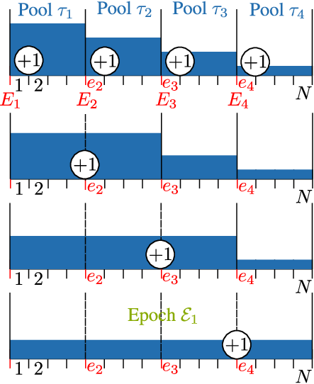
NDA: The worst case computational complexity for the NDA is produced when at every iteration of the algorithm it is observed that the water level is decreasing in some pool transition. Fig. 7 shows an example of how the algorithm proceeds for . In the first iteration a total of calls to are required. Then, in the second iteration, an additional call is performed to merge the first two epochs where it is observed that the water level is decreasing. As we are considering the worst case scenario, the resulting water-levels will be decreasing at some epoch transition and an additional call is required until all pools have been merged in a single epoch, therefore, the worst case computational complexity for the NDA is
| (34) | |||||
| (35) | |||||
| (36) |
where the first summation comes from the first iteration of the algorithm and the second one comes from merging the pools with decreasing water level, i.e., iterations from to . In (35), we have made the simplification of having equal length pools, i.e., , . The number of calls to is .
FSA: The FSA starts by assuming that the first epoch contains all the pools, then, it performs and checks whether the energy causality constraints are satisfied, which are not as we are considering the worst case scenario. Then, it removes the last pool from and tries again and so forth until just contains one pool and then the constraints must be satisfied. Therefore, a total of iterations are required to determine . Similarly, iterations are required to determine . The computational complexity at each iteration is summarized in Table II from where we can conclude that the worst case computational complexity of the FSA is
| (37) | |||||
| (38) |
where in (38) we have made the simplification of having equal length pools, i.e., , . As every iteration performs a call to , the total number of calls is .
| Iteration | Epoch | Complexity |
| Total | ||
| Total | ||
| Total | ||
E3 Computational complexity in the average case scenario
For the average case scenario, due to the inherent difficulty of determining the computational complexity measured in operations, we have just derived the complexity in terms of calls to the , i.e., . By doing this, we can see how the computational complexity is affected by the number of energy arrivals .
NDA: We start by analyzing the average performance of the NDA. Let , , be the probability that the water-level decreases at some pool transition. Let us assume equal probability at all pool transition , . Let be a random variable that, for a certain call to the NDA algorithm, denotes the number of calls to the . Note that the minimum number of calls to the is J and, from here, an additional call is produced every time that a water level decrease is produced. Observe that this additional number of calls is a binomial distribution of parameters and , i.e., . Therefore, and the mean and variance are
| (39) | |||||
| (40) |
FSA: Similarly for the FSA, let , , denote the probability that the -th energy causality constraint of the is not satisfied. We assume that this probability is equal for all the constraints , . Let be a random variable that, for a certain call to the FSA algorithm, denotes the number of calls to the . To determine for a general , let us first obtain for some specific values of as a function of the broken constraints. Note that up to constraints can be broken. In Tables III, IV, V, ✔ and ✘ denote that a certain constraint is satisfied or broken, respectively. For example, Table III shows when and the energy constraints that can be broken are in the transitions of , which is depicted in the first column, and , in the second column. Similarly, in Tables IV and V show the obtained values of for and , respectively. After carefully examining the previous tables, one may realize that there exists a fixed cost that depends on the number of broken constraints that is (at least, one call to is required before and after the broken constraint) and a variable cost that depends on the placement of the broken constraint. If the broken constraint is the last one the variable cost is . If it is the one before the last one, the variable cost is and so forth up to the case in which the broken constraint is the first energy causality constraint where the variable cost is . From this observation we can find for a general as
| (41) | |||||
| (42) | |||||
| (43) |
where in (43), we have used that the mean of a binomial distribution with parameters and is . Similarly, the variance of can be obtained through the variance of a binomial distribution as
| (44) |
This concludes the analysis of the computational complexity of the algorithms.
| J=3 | |||
| Constraint | Probability | ||
| ✔ | ✔ | 1 | |
| ✔ | ✘ | 3 | |
| ✘ | ✔ | 4 | |
| ✘ | ✘ | 6 | |
| J=4 | ||||
| Constraint | Probability | |||
| ✔ | ✔ | ✔ | 1 | |
| ✔ | ✔ | ✘ | 3 | |
| ✔ | ✘ | ✔ | 4 | |
| ✘ | ✔ | ✔ | 5 | |
| ✔ | ✘ | ✘ | 6 | |
| ✘ | ✔ | ✘ | 7 | |
| ✘ | ✘ | ✔ | 8 | |
| ✘ | ✘ | ✘ | 10 | |
| J=5 | |||||
| Constraint | Probability | ||||
| ✔ | ✔ | ✔ | ✔ | 1 | |
| ✔ | ✔ | ✔ | ✘ | 3 | |
| ✔ | ✔ | ✘ | ✔ | 4 | |
| ✔ | ✘ | ✔ | ✔ | 5 | |
| ✘ | ✔ | ✔ | ✔ | 6 | |
| ✔ | ✔ | ✘ | ✘ | 6 | |
| ✔ | ✘ | ✔ | ✘ | 7 | |
| ✘ | ✔ | ✔ | ✘ | 8 | |
| ✔ | ✘ | ✘ | ✔ | 8 | |
| ✘ | ✔ | ✘ | ✔ | 9 | |
| ✘ | ✘ | ✔ | ✔ | 10 | |
| ✔ | ✘ | ✘ | ✘ | 10 | |
| ✘ | ✔ | ✘ | ✘ | 11 | |
| ✘ | ✘ | ✔ | ✘ | 12 | |
| ✘ | ✘ | ✘ | ✔ | 13 | |
| ✘ | ✘ | ✘ | ✘ | 15 | |
F Properties of the reduction matrix
The reduction matrix, , was introduced in [18] and is defined as:
| (45) |
Note that from the structure of , in each column there is only one entry different than zero and it is equal to one. For instance, the matrices for and are:
The reduction matrix is designed so that
| (46) |
for . In this appendix, we summarize some additional properties of the reduction matrix:
Property 3.
Multiplication properties:
- •
Let , then the multiplication removes rows of .
- •
Let , then the multiplication adds rows of zeros to .
- •
Let , then the multiplication adds columns of zeros to .
- •
Let , then the multiplication removes columns of .
Proof:
The proof follows directly from the structure of the reduction matrix. ∎
Property 4.
Let , , then .
Proof:
See [18, Lemma A.2]. ∎
Property 5.
.
Proof:
The proof directly follows from setting and in Property 4. ∎
Property 6.
Let , then .
Proof:
The proof directly follows from setting in Property 4. ∎
Property 7.
Let , then .
Proof:
The Kronecker product expands the vector in a matrix that stacks diagonal matrices. Then, the multiplication by eliminates rows (see Property 3) so that the resulting matrix is . ∎
Property 8.
Let be a diagonal matrix, then
Proof:
From Property 3, removes rows from . Then, the product by the left by adds rows of zeros. As a result, zeroes rows of . Finally, the product with from the right removes columns. As is diagonal, the entries that are modified by multiplying from the left by are later removed by multiplying from the right by . Therefore, is equal than , which directly removes the columns. ∎
References
- [1] G. E. Moore et al., “Cramming more components onto integrated circuits,” Proceedings of the IEEE, vol. 86, no. 1, pp. 82–85, 1998.
- [2] T. M. Cover and J. A. Thomas, Elements of information theory. New York, NY, USA: Wiley-Interscience, 1991.
- [3] J. Yang and S. Ulukus, “Optimal packet scheduling in an energy harvesting communication system,” IEEE Trans. on Communications, no. 99, pp. 1–11, 2010.
- [4] K. Tutuncuoglu and A. Yener, “Optimum transmission policies for battery limited energy harvesting nodes,” IEEE Trans. on Wireless Communications, no. 99, pp. 1–10, 2010.
- [5] M. Gregori and M. Payaró, “Efficient data transmission for an energy harvesting node with battery capacity constraint,” in Proceedings of the IEEE GLOBECOM, Dec. 2011, pp. 1–6.
- [6] C. K. Ho and R. Zhang, “Optimal energy allocation for wireless communications with energy harvesting constraints,” IEEE Trans. on Signal Processing, vol. 60, no. 9, pp. 4808 –4818, Sep. 2012.
- [7] O. Ozel, K. Tutuncuoglu, J. Yang, S. Ulukus, and A. Yener, “Transmission with energy harvesting nodes in fading wireless channels: Optimal policies,” IEEE Journal on Selected Areas in Communications, vol. 29, no. 8, pp. 1732–1743, 2011.
- [8] O. Ozel, J. Yang, and S. Ulukus, “Optimal broadcast scheduling for an energy harvesting rechargeable transmitter with a finite capacity battery,” IEEE Trans. on Wireless Communications, vol. 11, no. 6, pp. 2193–2203, Jun. 2012.
- [9] ——, “Optimal transmission schemes for parallel and fading gaussian broadcast channels with an energy harvesting rechargeable transmitter,” Computer Communications, Elsevier, 2012.
- [10] M. A. Antepli, E. Uysal-Biyikoglu, and H. Erkal, “Optimal scheduling on an energy harvesting broadcast channel,” in WiOpt, 2011, pp. 197–204.
- [11] J. R. Magnus and H. Neudecker, Matrix differential calculus with applications in statistics and econometrics, ser. Wiley series in probability and statistics. New York: Wiley, 1999.
- [12] E. Telatar, “Capacity of multi-antenna Gaussian channels,” European transactions on telecommunications, vol. 10, no. 6, pp. 585–595, 1999.
- [13] G. D. Forney Jr and G. Ungerboeck, “Modulation and coding for linear gaussian channels,” IEEE Trans. on Information Theory, vol. 44, no. 6, pp. 2384–2415, 1998.
- [14] A. Lozano, A. M. Tulino, and S. Verdú, “Optimum power allocation for parallel Gaussian channels with arbitrary input distributions,” IEEE Trans. on Information Theory, vol. 52, no. 7, pp. 3033 – 3051, Jul. 2006.
- [15] D. Guo, S. Shamai, and S. Verdú, “Mutual information and minimum mean-square error in Gaussian channels,” IEEE Trans. on Information Theory, vol. 51, no. 4, pp. 1261 –1282, Apr. 2005.
- [16] D. P. Palomar and S. Verdú, “Gradient of mutual information in linear vector Gaussian channels,” IEEE Trans. on Information Theory, vol. 52, no. 1, pp. 141–154, 2006.
- [17] C. Xiao, Y. R. Zheng, and Z. Ding, “Globally optimal linear precoders for finite alphabet signals over complex vector Gaussian channels,” IEEE Trans. on Information Theory, vol. 59, no. 7, pp. 3301–3314, 2011.
- [18] M. Payaró and D. P. Palomar, “Hessian and concavity of mutual information, differential entropy, and entropy power in linear vector Gaussian channels,” IEEE Trans. on Information Theory, vol. 55, no. 8, pp. 3613 –3628, Aug. 2009.
- [19] ——, “On optimal precoding in linear vector Gaussian channels with arbitrary input distribution,” in IEEE International Symposium on Information Theory, ISIT., Jul. 2009, pp. 1085 –1089.
- [20] M. Lamarca, “Linear precoding for mutual information maximization in mimo systems,” in 6th IEEE International Symposium on Wireless Communication Systems, 2009, pp. 26–30.
- [21] S. Boyd and L. Vandenberghe, Convex optimization. Cambridge Univ Pr, 2004.
- [22] S. Verdú, “Spectral efficiency in the wideband regime,” IEEE Trans. on Information Theory, vol. 48, no. 6, pp. 1319 –1343, Jun. 2002.
- [23] D. Guo, Y. Wu, S. Verdú et al., “Estimation in Gaussian noise: Properties of the minimum mean-square error,” IEEE Trans. on Information Theory, vol. 57, no. 4, pp. 2371–2385, 2011.