AABC: approximate approximate Bayesian computation when simulating a large number of data sets is computationally infeasible

ABC methods have been based on rejection algorithms (Tavaré et al.,, 1997; Beaumont et al.,, 2002; Blum and François,, 2010), Markov chain Monte Carlo (Beaumont,, 2003; Marjoram et al.,, 2003; Bortot et al.,, 2007; Wegmann et al.,, 2009), and sequential Monte Carlo (Sisson et al.,, 2007; Sisson et al.,, 2009; Beaumont et al.,, 2009; Toni et al.,, 2009). Model selection using ABC (Pritchard et al.,, 1999; Fagundes et al.,, 2007; Grelaud et al.,, 2009; Blum and Jakobsson,, 2010; Robert et al.,, 2011), the choice of summary statistics when the likelihood is based on summary statistics instead of the full data (Joyce and Marjoram,, 2008; Wegmann et al.,, 2009; Nunes and Balding,, 2010; Fearnhead and Prangle,, 2012), and the equivalence of posterior distributions targeted in different ABC methods (Wilkinson,, 2008; Sisson et al.,, 2010) have also been investigated.

ABC methods have had a considerable effect on model-based inference in disciplines that rely on genetic data, particularly data shaped by diverse evolutionary, demographic, and environmental forces. Example applications have included problems in the demographic history of populations (Pritchard et al.,, 1999; François et al.,, 2008; Verdu et al.,, 2009; Blum and Jakobsson,, 2010) and species (Estoup et al.,, 2004; Plagnol and Tavaré,, 2004; Becquet and Przeworski,, 2007; Fagundes et al.,, 2007; Wilkinson et al.,, 2010), as well as problems in the evolution of cancer cell lineages (Tavaré,, 2005; Siegmund et al.,, 2008) and the evolution of protein networks (Ratmann et al.,, 2009). Other applications outside of genetics have included inference on the physics of stereological extremes (Bortot et al.,, 2007), the ecology of tropical forests (Jabot and Chave,, 2009), dynamical systems in biology (Toni et al.,, 2009), and small-world network disease models (Walker et al.,, 2010). ABC methods have been reviewed by Marjoram and Tavaré, (2006), Cornuet et al., (2008), Beaumont et al., (2009), Beaumont, (2010), Csilléry et al., (2010), and Marin et al., (2011).

An informal categorization of the information available about the likelihood function is helpful to illustrate the class of models in which ABC methods are most useful. First, exact inference on the posterior distribution of the parameters is possible only if the likelihood function is analytically available. Second, if the likelihood function is not analytically available but can be evaluated up to a constant given a parameter value, then standard computational methods such as rejection algorithms can sample the posterior distribution. In this case, inference is exact up to a Monte Carlo error due to sampling from the posterior. Third, if the likelihood function cannot be evaluated, but data sets can feasibly be simulated from the model, then ABC methods sample the posterior distribution using approximations on the data space in addition to a Monte Carlo error due to sampling.

Although ABC methods sample the posterior distribution of parameters without evaluating the likelihood function, they are computationally intensive. Adequately sampling a posterior distribution of a parameter by ABC requires many random realizations from the prior distribution of the parameter and the sampling distribution of the data. Simulating from the prior is straightforward, but the computational cost of simulating a data set from the mechanistic model increases quickly with the complexity and number of stochastic processes involved. Henceforth, we refer to statistical models in which not only evaluating the likelihoods is difficult but also simulating a large number of data sets is computationally infeasible as limited-generative models. When a model is limited-generative and only a small number of data sets can be simulated from the model, likelihoods cannot be assessed using ABC and hence, the posterior distribution of parameters cannot be adequately sampled.

In this article, we introduce approximate approximate Bayesian computation (AABC), a class of methods that perform inference on model-specific parameters of limited-generative models when standard ABC methods are computationally infeasible to apply. In AABC, the idea of assessing the likelihoods approximately using simulated data sets is taken one step further than in ABC. AABC methods make approximations on the parameter space and the model space in addition to standard ABC approximations on the data space. In conjunction with Bayesian resampling methods, these approximations help us overcome the computational intractability associated with simulating data from a limited-generative model (Figure 1).

Our key innovation is to condition on a limited number of data sets that can be feasibly simulated from the limited-generative model and to employ a non-mechanistic statistical model to simulate a large number of data sets. We set up the non-mechanistic model based on empirical distributions of the limited number of data sets simulated from the mechanistic model. Since the data values from the limited number of simulated data sets are used to construct new random data sets by resampling methods, it is computationally inexpensive to simulate a large number of data sets in AABC. The AABC approach allows a researcher to allocate a fixed computer time to simulating a limited number of data sets from the limited-generative model, thus making otherwise challenging likelihood-based inference attainable.

Intuitively, the information conditioned upon by the non-mechanistic model increases with the number of data sets simulated from the mechanistic model, and the expected accuracy of inference obtained by AABC methods increases. We formalize this intuition by showing that the posterior distribution of parameters obtained by AABC converges to the corresponding posterior distribution obtained by standard ABC, as the sample size of the observed data set and the number of data sets simulated from the limited-generative model increase simultaneously.

AABC methods utilize the established machinery of ABC methods in sampling the posterior distribution of the parameters. Therefore, standard approximations on the data space involved in an ABC method—which facilitate the sampling of the posterior distribution—apply to AABC methods as well. We now briefly review these approximations in the context of ABC by rejection algorithms.

Two approximations are involved in substituting $P_{\theta}$ with $Q_{\theta}.$ First, $\mathcal{Z}_{n,m}$ includes only $m$ parameter values $\theta_{1},\theta_{2},...,\theta_{m}$ under which data sets are simulated from $P_{\theta}$. After obtaining $\mathcal{Z}_{n,m},$ for any new parameter value $\theta$ from the prior distribution under which we want to simulate a new data set, we substitute $\theta$ with $\tilde{\theta}$ such that $(\tilde{{\bf x}},\tilde{\theta})\in\mathcal{Z}_{n,m}.$ The value $\tilde{\theta}$ has the minimum Euclidean distance to the value $\theta$ among all parameter values in $\mathcal{Z}_{n,m}.$ More precisely, $\tilde{\theta}=\displaystyle{\mathop{\mbox{arg\;min}}_{\theta_{j}\in\mathcal{Z}_{n,m}}}||\theta_{j}-\theta||.$ In essence, this approximation is equivalent to replacing the sampling distribution of the data set $P_{\theta}$ with the sampling distribution $P_{\tilde{\theta}}$; we call this an approximation on the parameter space. However, this parameter space approximation is not sufficient to simulate data sets efficiently, since the model $P_{\tilde{\theta}}$ is still limited-generative after this substitution.

As a second approximation, we substitute the model $P_{\tilde{\theta}}$ with the empirical distribution of the data set $\tilde{{\bf x}}$ that has already been simulated from $P_{\tilde{\theta}}$ as $(\tilde{{\bf x}},\tilde{\theta})\in\mathcal{Z}_{n,m}.$ Here, we assume a positive probability mass only on the data values observed in the set $\tilde{{\bf x}}.$ We call this an approximation on the model space because the model $P_{\tilde{\theta}}$ is substituted with the empirical distribution of a data set simulated from $P_{\tilde{\theta}}.$

To simulate a new data set ${\bf x}$ in AABC, we utilize a vector of positive auxiliary parameters $\textrm{\boldmath$\phi$}=(\phi_{1},\phi_{2},...,\phi_{n}),$ that satisfy $\sum_{i=1}^{n}\phi_{i}=1.$ We let $\phi_{i}$ be the probability that a random data value $x_{j}\in{\bf x}$ is equal to a given value $\tilde{x}_{i}$ found in the data set $\tilde{{\bf x}}=(\tilde{x}_{1},\tilde{x}_{2},...,\tilde{x}_{n}).$ The premise is that the sample $\tilde{{\bf x}}$ simulated under $\tilde{\theta}$ provides information about the model $P_{\tilde{\theta}},$ and by an approximation of $\theta$ to $\tilde{\theta}$ on the parameter space, about $P_{\theta}$.

If we denote the approximate sampling distribution of a data set ${\bf x}=(x_{1},x_{2},...,x_{n})$ by $Q_{\theta},$ its joint probability mass function is

where $q({\bf x}|\textrm{\boldmath$\phi$},\tilde{{\bf x}})={n\choose n_{1}\;n_{2}\;\cdots\;n_{k}}\prod_{j=1}^{n}\prod_{i=1}^{n}\phi_{i}^{\mathbf{I}_{\{x_{j}=\tilde{x}_{i}\}}},$ and $\mathbf{I}_{\{\theta,\tilde{\theta}\}}$ is 1 if $\tilde{\theta}\in\mathcal{Z}_{n,m}$ is the closest value to $\theta$ in the Euclidean sense and is 0 otherwise. Here, $n_{i}$ is the number of times $\tilde{x}_{i}$ observed in the new sample ${\bf x},$ $k$ is the number of distinct data values observed in the data set ${\bf x},$ and $\mathbf{I}_{\{x_{j}=\tilde{x}_{i}\}}$ is 1 if $x_{j}=\tilde{x}_{i}$ and is 0 otherwise. The distribution $q({\bf x}|\textrm{\boldmath$\phi$},\tilde{{\bf x}})$ is that of an IID sample ${\bf x}=(x_{1},x_{2},...,x_{n}),$ where $x_{j}$ is drawn from the values $(\tilde{x}_{1},\tilde{x}_{2},...,\tilde{x}_{n})$ with probabilities $(\phi_{1},\phi_{2},...,\phi_{n}).$

The probability vector $\phi$ is a parameter of the model conditional on $\tilde{{\bf x}},$ and thus, we need to posit a prior distribution on $\textrm{\boldmath$\phi$}.$ As a natural prior on probabilities, we let the prior distribution $\pi(\textrm{\boldmath$\phi$})$ on $\phi$ be the symmetric Dirichlet distribution on the $(n-1)$-dimensional simplex $\Phi,$ with hyperparameters (1,1,…,1) and a uniform probability density function proportional to $1.$ This choice assigns equal weight to all distributions placing positive probability mass on the data points $\tilde{x}_{i}\in\tilde{{\bf x}}.$ Further, it assigns zero posterior probability to data values unobserved in the sample $\tilde{{\bf x}},$ thereby avoiding difficulties created by such values in the likelihood (Rubin,, 1981; Owen,, 1990).

To distinguish the parameter and data set realizations in $\mathcal{Z}_{n,m}=\{({\bf x}_{i},\theta_{i})\}_{i=1}^{m}$ from the parameter and data sets simulated using AABC, we use starred versions of each quantity to denote specific values simulated in AABC. For example, as the sampling distribution $P_{\theta_{i}}$ delivers a data set ${\bf x}_{i}$ under a given parameter value $\theta_{i}$ in the ABC procedure of Algorithm 2, the sampling distribution $Q_{\theta^{*}_{i}}$ delivers a data set ${\bf x}^{*}_{i}$ under a given parameter value $\theta^{*}_{i}$ simulated from its prior distribution (see Figure 4 for notation).

The sampling distribution $Q_{\theta}$ utilizes the information available in the set of realizations $\mathcal{Z}_{n,m}$ through the parameter $\textrm{\boldmath$\phi$},$ since the prior distribution of $\phi$ conditions on $(\tilde{{\bf x}},\tilde{\theta})\in\mathcal{Z}_{n,m}$ and thus on the set $\mathcal{Z}_{n,m}.$ In this sense, the available realizations $\mathcal{Z}_{n,m}$ are used as fixed background information about $P_{\theta},$ and inferences using the substitute model $Q_{\theta}$ are conditional on the simulated sets $\mathcal{Z}_{n,m}.$

In sampling the approximate posterior distribution of $\theta$ by AABC methods, we use the two ABC approximations described in Section 2. First, we substitute each data instance ${\bf x}$ with summary statistics $\textrm{\boldmath$s$}.$ Second, we use an acceptance condition with tolerance $\epsilon,$ employing the Euclidean distance to measure the proximity of the summary statistics calculated from the observed and simulated data, as in equation 1. If we let $\theta^{*}_{j}$ be a new parameter value simulated from its prior distribution after obtaining the set $\mathcal{Z}_{n,m},$ in AABC we accept the parameter values $\theta^{*}_{j}$ producing summary statistics $\textrm{\boldmath$s$}^{*}_{j}$ that satisfy the condition $||\textrm{\boldmath$s$}^{*}_{j}-\textrm{\boldmath$s$}_{o}||<\epsilon$ as being draws from the posterior distribution. This acceptance condition corresponds to a uniform kernel, which we use throughout this article, although like ABC, AABC can employ other kernels to obtain smooth weighting of $\textrm{\boldmath$s$}^{*}_{j}$ values by their distance from $\textrm{\boldmath$s$}_{o}.$ Substituting $P_{\theta}$ with $Q_{\theta}$ involves replacing $p({\bf x}|\theta)$ in expression 2 with expression 3 and adjusting the normalizing constant accordingly. The approximate posterior distribution sampled by an AABC method is

where $C_{Q_{\theta}}=\int_{\Theta}\int_{\mathcal{X}}\mathbf{I}_{\{||\textrm{\boldmath$s$}-\textrm{\boldmath$s$}_{o}||<\epsilon\}}\left[\int_{\Phi}q({\bf x}|\textrm{\boldmath$\phi$},\tilde{{\bf x}})\pi(\textrm{\boldmath$\phi$})\;d\textrm{\boldmath$\phi$}\;\mathbf{I}_{\{\theta,\tilde{\theta}\}}\right]\pi(\theta)\;d{\bf x}\;d\theta$ is the normalizing constant.

The AABC approach is sensible in that as the limited generative model increasingly permits a larger number of simulated data sets, for large sample sizes the posterior distribution obtained by an AABC method approaches the same distribution as the posterior distribution obtained by an ABC method. We codify this claim with a theorem.

The structure of AABC algorithms sampling the posterior distribution in expression 4 can be conveniently summarized in three parts, as shown in AABC by a rejection algorithm (Figure 5). In Algorithm 2, Part I involves obtaining a limited number of realizations from the joint distribution of the parameter and the data from the limited-generative model $P_{\theta}.$ Part I simply involves the application of steps 1 and 2 from Algorithm 1, but only for $m$ iterations. Part II involves simulating a new parameter value $\theta^{*}_{i}$ from its prior distribution (step 4) and then simulating a data set ${\bf x}^{*}_{i}$ from the model $Q_{\theta^{*}_{i}}$ (steps 5, 6, 7), conditional on $\mathcal{Z}_{n,m}$ obtained in Part I. Part III involves comparing the summary statistics $\textrm{\boldmath$s$}^{*}_{i}$ calculated from the simulated data set ${\bf x}^{*}_{i}$ with the summary statistics $\textrm{\boldmath$s$}_{o}$ calculated from the observed data set ${\bf x}_{o},$ to accept or reject the parameter value $\theta^{*}_{i}.$ The calculation and comparison of summary statistics follows the same procedure as in steps 3 and 4 of Algorithm 1. Hence, Part II of AABC by rejection has the novel steps 5, 6, and 7, whereas Parts I and III use the machinery of ABC by rejection from Algorithm 1.

We can show that Algorithm 2 samples the correct posterior distribution $\pi_{\epsilon}(\theta|{\bf x}_{o},Q_{\theta}).$ The probability of sampling a parameter value $\theta$ in Algorithm 2 is proportional to

where the third line follows from the fact that the expression on the second line is the product of the likelihood under the model $Q_{\theta}$ and the prior, and therefore it is proportional to the posterior distribution of parameters based on the model $Q_{\theta}.$

We simulated a reference set with $M=10^{5}$ realizations $\{({\bf x}_{1},\theta_{1}),({\bf x}_{2},\theta_{2}),...,({\bf x}_{10^{5}},\theta_{10^{5}})\},$ by first generating $\theta_{i}\sim\pi(\theta)$ and then simulating a data set ${\bf x}_{i}\sim P_{\theta_{i}}.$ We then sampled 1000 pairs $({\bf x}_{i},\theta_{i})$ from the reference set, uniformly at random without replacement. Thus, we selected 1000 “true” parameter values $\theta_{i},$ along with corresponding test data sets ${\bf x}_{i}$ generated under each value $\theta_{i}$ from the model $P_{\theta_{i}}$. Further, we built the sets $\mathcal{Z}_{n,m},$ with $m=10^{2},5\times 10^{2},10^{3},5\times 10^{3},10^{4},5\times 10^{4},10^{5}$ by sampling the reference set uniformly at random without replacement for $m<10^{5},$ and taking all the realizations in the reference set for $m=M=10^{5}.$ The sample size $n$ of the data is described in each relevant example.

On each test data set, we performed AABC by rejection sampling (Algorithm 2) using each set $\mathcal{Z}_{n,m}.$ In example 1, where our goal is to compare the performance of the AABC and ABC approaches, we performed ABC analyses by rejection sampling (Algorithm 1) using the same sets $\mathcal{Z}_{n,m}.$ For all analyses, we obtained a sample from the joint posterior distribution of the parameter vector $\theta$ by accepting the parameter vector values that generated data whose summary statistics were in the top $1$ percentile with respect to the statistics calculated from the test data set, in the sense of equation 1. Compared to the approach of fixing the $\epsilon$ cutoff, accepting parameter vectors that generate data whose summary statistics are in a top percentile has the advantage that a desired number of samples from the posterior is always obtained given a total fixed number of proposed parameter values. This approach is often preferred by ABC practitioners and is convenient in our case for comparing ABC and AABC.

We assessed the accuracy of the posterior samples for each component of the parameter vector $\theta$ separately, using the root sum of squared error for standardized parameter values accepted in the posterior sample. For a generic scalar parameter $\alpha,$ the root sum of squared errors is given by $\textrm{RSSE}=(1/r)\sqrt{\sum_{j=1}^{r}(\alpha_{j}-\alpha_{T})^{2}/\textrm{Var}(\mathbf{\alpha})},$ where $\mathbf{\alpha}=(\alpha_{1},\alpha_{2},...,\alpha_{r})$ are $r$ accepted values in the posterior sample, $\alpha_{T}$ is the true parameter value, and $\textrm{Var}(\mathbf{\alpha})$ is the variance of the set of $r$ values. We report the mean RSSE over 1000 test data sets as $\textrm{RMSE}=(1/1000)\sum_{i=1}^{1000}\textrm{RSSE}_{i}$ (see Nunes and Balding, (2010)).

In this section, we consider inference from the stationary distribution of allele frequencies in the diffusion approximation to a Wright-Fisher model with symmetric balancing selection and mutation (Wright,, 1949). If we let $a_{i}>0,$ with $i=1,2,...,K,$ and $\sum_{i=1}^{K}a_{i}=1,$ and denote the frequency of allelic type $i$ in the population at a genetic locus, the joint probability density function of allele frequencies $x=(a_{1},a_{2},...,a_{K})$ is $f(x|\sigma,\mu)=c(\sigma,\mu)^{-1}\exp(-\sigma\sum_{i=1}^{K}a_{i}^{2})\prod_{i=1}^{K}a_{i}^{\mu/K-1}.$ Parameters $\sigma$ and $\mu$ determine the population-scaled strength of balancing selection and the mutation rate, respectively. A data set of observed allele frequencies is a random sample of $n$ draws from the population frequencies $f(x|\sigma,\mu).$

ABC methods are well-suited for inference from this model for three reasons. First, the statistics $\sum_{j=1}^{K}a_{j}^{2}$ and $-\sum_{j=1}^{K}\log a_{j}$ are jointly sufficient for parameters $\sigma$ and $\mu,$ and no information loss occurs in dimension reduction to the summary statistics. Second, the parameter-dependent normalizing constant $c(\sigma,\mu)$ is hard to calculate, and performing likelihood-based inference on $\sigma$ and $\mu$ is therefore difficult. Third, a method specifically designed to simulate data sets from $f(x|\sigma,\mu)$ is readily available (Joyce et al.,, 2012), and performing ABC is therefore straightforward. For simplicity, we assume 100 loci with the same true parameter values, each with $K=4,$ and that the allele frequencies at each locus are independent of the allele frequencies at other loci. Thus, the joint probability density function of allele frequencies for 100 loci is equal to the product of probability density functions across loci. We choose uniform prior distributions, on $(0.1,10)$ for the mutation rate $(\mu),$ and on $(0,50)$ for the selection parameter $(\sigma)$.

Results. Posterior samples model parameters $(\sigma,\mu)$ obtained by ABC and AABC using a typical data set are given in Figure 6. In analyses with $m=10^{2},5\times 10^{2},10^{3}$ or $5\times 10^{3}$ simulated data sets, few samples are accepted with ABC, and thus, little mass is observed in ABC histograms (black). For small $m,$ ABC does not produce an adequate sample size from the posterior distribution of parameters. AABC, however, produces a posterior sample of size $10^{3}$ for any $m,$ because $10^{5}$ data sets are simulated from the non-mechanistic model (Algorithm 2, steps 5, 6, 7) and the top 1 percentile are accepted as belonging to the approximate posterior distribution. The histograms obtained by AABC recover the true value reasonably well (Figure 6). The RMSE values in AABC procedures are approximately constant with increasing $m.$ For $m=10^{2},5\times 10^{2},10^{3},5\times 10^{3},10^{4},5\times 10^{4},$ and $10^{5}$ simulated data sets, the RMSE values for parameter $\mu$ are 5.988, 5.932, 6.012, 6.086, 6.125, 6.078, and 6.088 respectively, close to the RMSE of 5.290 obtained by a standard ABC approach using $M=10^{5}$ simulated data sets from the mechanistic model. The RMSE values in the last column of Figure 6 show that an AABC approach produces posterior samples that have on average greater variance than posterior samples obtained from ABC with the same large number of realizations. Here, greater variance in posterior samples obtained by AABC is a result of simulating data sets in AABC by resampling the observed data values that are found only in the $m$ realizations in $\mathcal{Z}_{n,m}.$ Consider two parameter values $\theta^{*}_{1}$ and $\theta^{*}_{2}$ for which data sets ${\bf x}^{*}_{1}$ and ${\bf x}^{*}_{2}$ are simulated in the AABC approach by steps 5, 6, 7 of Algorithm 2 such that the parameter value $\tilde{\theta}\in\mathcal{Z}_{n,m}$ closest to both $\theta^{*}_{1}$ and $\theta^{*}_{2}$ is the same value. The data sets ${\bf x}^{*}_{1}$ and ${\bf x}^{*}_{2}$ can include only the data values observed in $\tilde{{\bf x}}$ of the pair $(\tilde{{\bf x}},\tilde{\theta})\in\mathcal{Z}_{n,m}.$ On average, ${\bf x}^{*}_{1}$ and ${\bf x}^{*}_{2}$ share more observations in common than two data sets simulated from the respective mechanistic models $P_{\theta^{*}_{1}}$ and $P_{\theta^{*}_{2}}.$ Therefore, each data set simulated in the AABC approach using $Q_{\theta}$ is expected to be less able to distinguish between different parameter values than the independent data sets simulated in the ABC approach using $P_{\theta}.$ This situation results in relatively flat likelihoods and hence posterior samples with larger variance.

Models in which hybrid populations are founded by, and receive genetic contributions from, multiple source populations are of interest in describing the demographic history of admixture. Stochastic models including admixture often result in likelihoods that are difficult to calculate, and statistical methods capable of performing inference on admixture rates have received much attention for their implications on topics ranging from human evolution to conservation ecology (Falush et al.,, 2003; Tang et al.,, 2005; Buerkle and Lexer,, 2008). Here, we consider inference on admixture rates from a mechanistic model of Verdu and Rosenberg, (2011). We use reported estimates of individual admixture as data.

We consider a model of admixture for a diploid hybrid population of constant size $N,$ founded at some known $t$ generations in the past with contributions from source populations A and B. We follow the distribution of admixture fractions of individuals in the hybrid population at a given genetic locus. Each generation, the admixture fraction for each individual in the hybrid population is obtained as the mean of the admixture fractions of its parents. The parents are chosen independently of each other, from source population A, source population B, or the hybrid population of the previous generation with probabilities $p_{A},p_{B},$ and $p_{H},$ respectively ($p_{A}+p_{B}+p_{H}=1$). In the special case of the founding generation, $p_{H}=0,$ and we assume $p_{A}=p_{B}=0.5.$ Individuals from source populations A and B are assigned admixture fractions of $1$ and $0$ respectively. For example, if both parents of an individual in the hybrid population of the founding generation are from source population A, that individual has admixture fraction $(1+1)/2=1.$ If both parents are from population 2, the admixture fraction is $(0+0)/2=0,$ and if one parent is from population 1 and the other is from population B, then the admixture fraction is $(1+0)/2=0.5.$ The distribution of the admixture fraction in the hybrid population is propagated in this manner for $t$ generations until the present, in which a sample of $n$ individuals is obtained from the resulting distribution (Figure 7). Our goal is to estimate the admixture rates $(p_{A},p_{B},p_{H}),$ given the individual admixture fractions estimated from observed genetic data.

We apply the AABC approach using individual admixture fractions from $n=604$ individuals from Central African Pygmy populations reported by Verdu et al., (2009), with an assumed constant population size of $N=10^{4}.$ This assumption differs slightly from the original model in Verdu and Rosenberg, (2011) in that a finite population size is assumed, so that only $10^{4}$ admixture fraction values are allowed in the population at any given generation. We assume that an admixture event with contributions from two ancestral source populations started at the mean estimate of $t=771$ generations ago (Verdu et al.,, 2009) with a generation time of 25 years, and that it continued until the present. Source population A refers to an ancestral Pygmy population, and source population B refers to an ancestral non-Pygmy population. The feature of this model relevant to our method is the computational intractability of simulating data sets. For each set of parameter values $(p_{A},p_{B},p_{H})$ simulated from the priors, the distribution of admixture fractions is discrete on a support of a number of admixture fraction values that doubles each generation, and this distribution evolves for 771 generations. A random sample of admixture fraction values comparable to the values calculated from the observed data set is obtained from the distribution of the present generation. Simulating a large number of data sets under this model with such a large number of generations is computationally infeasible, and standard ABC is impractical. We thus perform AABC by rejection (Algorithm 2) using $m=10^{4}$ realizations from this model. We assume a Dirichlet prior with hyperparameters $(1,1,1)$ on parameters $(p_{A},p_{B},p_{H}).$

We also assessed the contribution of the approximations on the parameter and model spaces in the AABC approach to the RMSE separately, with a simulation study using a small number of generations ($t=30$), where simulating data sets from the mechanistic model is feasible. First, we performed AABC with rejection as in Algorithm 2 with 1000 “true” data sets using $m=10^{2},5\times 10^{2},10^{3},5\times 10^{3},10^{4},5\times 10^{4},$ and $10^{5}$ realizations from the model, and we calculated the RMSE for $p_{A},p_{B},$ and $p_{H}$ over 1000 “true” data sets as described in Section 4.1. This AABC analysis includes error due to approximations on the parameter space and on the model space. Second, we performed an AABC analysis with the same set of $m$ realizations, by including the error only due to the approximation on the parameter space. We achieved this by running Algorithm 2 up through step 5, and then simulating data sets from the mechanistic model by substituting steps 6 and 7 of Algorithm 2 with step 2 of Algorithm 1, the standard ABC approach by rejection. By this substitution, all data sets are simulated from the mechanistic model, but each data set is obtained using a parameter vector $(\tilde{p}_{A},\tilde{p}_{B},\tilde{p}_{H})$ found in step 5 of Algorithm 2. In this procedure, the error due to the approximation on the model space is eliminated, because data sets are simulated from the correct mechanistic model and not by resampling from the available realizations in $\mathcal{Z}_{n,m}$. However, this procedure includes error due to the approximation on the parameter space, because each data set is simulated not under the correct proposed parameter value, but under the parameter value $(\tilde{p}_{A},\tilde{p}_{B},\tilde{p}_{H}),$ the closest value to the correct proposed value that can be found in $\mathcal{Z}_{n,m}.$ We compared the RMSE of the AABC procedure involving the approximation on both the parameter and model spaces and the RMSE of the AABC procedure involving only the approximation on the parameter space to the RMSE obtained from a standard ABC approach. For these two AABC procedures, we also compared the percent excess in RMSE, defined as the ratio of the absolute difference in RMSE of the AABC and standard ABC approaches to the RMSE of the standard ABC approach, expressed as a percent.

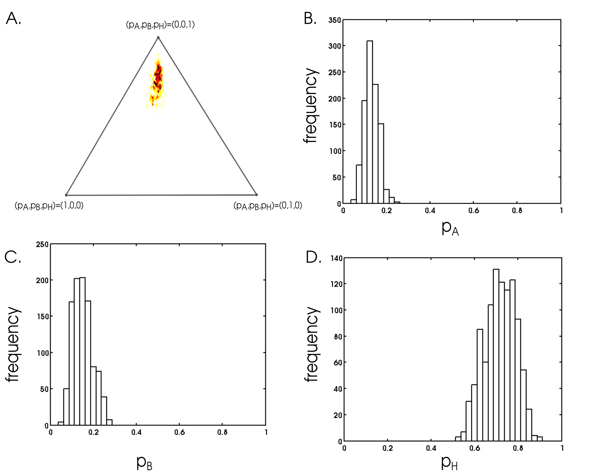
Results. The individual admixture fractions calculated from the Pygmy data carry substantial information about the admixture parameters $p_{A},p_{B},$ and $p_{H},$ since the joint posterior distribution is concentrated in a relatively small region of the 3-dimensional unit simplex on which $(p_{A},p_{B},p_{H})$ sits (Figure 8A). The marginal posterior distributions (Figure 8B, 8C, and 8D) have means $p_{A}=0.151,\;p_{B}=0.132,$ and $p_{H}=0.717.$ These values are interpreted as contribution of genetic material of 15.1% from the ancestral Pygmy population (source population A), 13.2% from the ancestral Non-Pygmy population (source population B), and 71.7% from the hybrid population to itself at each generation, over $771$ generations of constant admixture.

For the simulation study with $t=30$ generations and 1000 “true data” sets, the RMSE values from AABC analyses decrease with increasing $m$ (Figure 9A, 9B, 9C). Further, as $m$ increases, the error due to the approximation on the parameter space decreases (Figure 9D last column), due to the fact that for large $m,$ the difference decreases between the closest parameter value chosen at step 5 of Algorithm 2 and the correct parameter value under which we want to simulate a data set. In fact, the RMSE from the AABC analysis with $m=10^{5}$ realizations and approximation only on the parameter space and the RMSE from the standard ABC approach are virtually indistinguishable (Figure 9A, 9B, 9C, red star). For $m=10^{3},$ the AABC analysis with approximations on the parameter and model spaces has a percent excess RMSE of 13.81%, whereas AABC analysis including only the approximation on the parameter space has excess RMSE of 6.61%. That is, at $m=10^{3},$ approximately half of the excess RMSE in the AABC approach with respect to the standard ABC analysis comes from the error due to the approximation on the parameter space and half arises due to the approximation on the model space.

References

- Aeschbacher et al., (2012) Aeschbacher, S., Futschik, A., and Beaumont, M.A. (2012), “A novel approach for choosing summary statistics in approximate Bayesian computation,” Genetics, 192, 1027–1047.
- Beaumont, (2003) Beaumont, M.A. (2003), “Estimation of population growth or decline in genetically monitored populations,” Genetics, 164, 1139–1160.
- Beaumont, (2010) Beaumont, M.A. (2010), “Approximate Bayesian computation in evolution and ecology,” Annual Reviews of Ecology, Evolution and Systematics, 41, 379–406.
- Beaumont et al., (2002) Beaumont, M.A., Zhang, W., and Balding, D.J. (2002), “Approximate Bayesian computation in population genetics,” Genetics, 162, 2025–2035.
- Beaumont et al., (2009) Beaumont, M.A., Cornuet, J.-M., Marin, J.-M., and Robert, C.P. (2009), “Adaptive approximate Bayesian computation,” Biometrika, 96, 983–990.
- Becquet and Przeworski, (2007) Becquet, C., and Przeworski, M. (2007), “A new approach to estimate parameters of speciation models with application to apes,” Genome Research, 17, 1505–1519.
- Blum and François, (2010) Blum, M.G.B., and François, O. (2010), “Non-linear regression models for approximate Bayesian computation,” Statistics and Computing, 20, 63–73.
- Blum and Jakobsson, (2010) Blum, M.G.B., and Jakobsson, M. (2010), “Deep divergences of human gene trees and models of human origins,” Molecular Biology and Evolution, 28, 889–898.
- Bortot et al., (2007) Bortot, P., Coles, S., and Sisson, S.A. (2007), “Inference for stereological extremes,” Journal of the American Statistical Association, 102, 84–92.
- Buerkle and Lexer, (2008) Buerkle, C.A. and Lexer, C. (2008), “Admixture as the basis for genetic mapping,” Trends in Ecology and Evolution, 23, 686–694.
- Cornuet et al., (2008) Cornuet, J.-M., Santos, F., Beaumont, M.A., Robert, C.P., Marin, J.-M., Balding, D.J., Guillemaud, T., and Estoup, A. (2008), “Inferring population history with DIY ABC: a user-friendly approach to approximate Bayesian computation,” Bioinformatics, 24, 2713–2719.
- Csilléry et al., (2010) Csilléry, K., Blum, M.G.B., Gaggiotti, O.E., and François, O. (2010), “Approximate Bayesian computation (ABC) in practice,” Trends in Ecology and Evolution, 25, 410–418.
- Diggle and Gratton, (1984) Diggle, P.J., and Gratton, R.J. (1984), “Monte Carlo methods of inference for implicit statistical models,” Journal of the Royal Statistical Society, Series B 46, 193–227.
- Estoup et al., (2004) Estoup, A., Beaumont, M.A., Sennedot, F., Moritz, C., and Cornuet, J.-M. (2004), “Genetic analysis of complex demographic scenarios: spatially expanding populations of the cane toad, Bufo marinus,” Evolution 58, 2021–2036.
- Fagundes et al., (2007) Fagundes, N.J.R., Ray, N., Beaumont, M.A., Neuenschwander, S., Salzano, F.M., Bonatto, S.L., and Excoffier, L. (2007), “Statistical evaluation of alternative models of human evolution,” Proceedings of the National Academy of Sciences, 104, 17614–17619.
- Falush et al., (2003) Falush, D., Stephens, M., and Pritchard, J.K. (2003), “Inference of population structure using multilocus genetic data: linked loci and correlated allele frequencies,” Genetics, 164, 1567–1587.
- Fearnhead and Prangle, (2012) Fearnhead, P., and Prangle, D. (2012), “Constructing summary statistics for approximate Bayesian computation: semi-automatic approximate Bayesian computation,” Journal of the Royal Statistical Society, Series B, 74, 1–28.
- François et al., (2008) François, O., Blum, M.G.B., Jakobsson, M., and Rosenberg, N.A. (2008), “Demographic history of European populations Arabidopsis thaliana,” PLoS Genetics, 4, e1000075.
- Grelaud et al., (2009) Grelaud, A., Robert, C.P., Marin, J.-M., Rodolphe, F., and Taly, J.-F. (2009), “ABC likelihood-free methods for model choice in Gibbs random fields,” Bayesian Analysis, 4, 317–336.
- Jabot and Chave, (2009) Jabot, F., and Chave, J. (2009), “Inferring the parameters of the neutral theory of biodiversity using phylogenetic information and implications for tropical forests,” Ecology Letters, 12, 239–248.
- Joyce et al., (2012) Joyce, P., Genz, A., and Buzbas, E.O. (2012), “Efficient simulation and likelihood methods for non-neutral multi-allele models,” Journal of Computational Biology, 19, 650–661.
- Joyce and Marjoram, (2008) Joyce, P., and Marjoram, P. (2008), “Approximately sufficient statistics and Bayesian computation,” Statistical Applications in Genetics and Molecular Biology, 7, Article 26.
- Kotz et al., (2000) Kotz, S., Balakrishnan, N., and Johnson, N.L. (2000), Continuous Multivariate Distributions, Second Ed., Wiley-Interscience, New York.
- Leuenberger and Wegmann, (2010) Leuenberger, C., and Wegmann, D. (2010), “Bayesian computation and model selection without likelihoods,” Genetics, 184, 243–252.
- Liu, (2008) Liu, J.S. (2008), Monte Carlo Strategies in Scientific Computing, Springer, New York.
- Marjoram et al., (2003) Marjoram, P., Molitor, J., Plagnol, V., and Tavaré, S. (2003), “Markov chain Monte Carlo without likelihoods,” Proceedings of the National Academy of Sciences, 100, 15324–15328.
- Marjoram and Tavaré, (2006) Marjoram, P., and Tavaré, S. (2006), “Modern computational approaches for analysing molecular genetic variation data,” Nature Reviews Genetics, 7, 759–770.
- Marin et al., (2011) Marin, J.-M., Pudlo, P., Robert, C.P., and Ryder, R. (2011), “Approximate Bayesian computational methods,” Statistics and Computing, 22, 1167–1180.
- Nunes and Balding, (2010) Nunes, M.A., and Balding, D.J. (2010), “On optimal selection of summary statistics for approximate Bayesian computation,” Statistical Applications in Genetics and Molecular Biology, 34, Article 34.
- Owen, (1990) Owen, A. (1990), “Empirical likelihood ratio confidence regions,” Annals of Statistics, 18, 90–120.
- Plagnol and Tavaré, (2004) Plagnol, V., and Tavaré, S. (2004), “Approximate Bayesian computation and MCMC,” in Monte Carlo and Quasi-Monte Carlo Methods, ed. H. Niederreiter, Springer-Verlag, pp 99-114.
- Pritchard et al., (1999) Pritchard, J.K., Seielstad, M.T., Perez-Lezaun, A., and Feldman, M.W. (1999), “Population growth of human Y chromosomes: a study of Y chromosome microsatellites,” Molecular Biology and Evolution, 16, 1791–1798.
- Ratmann et al., (2009) Ratmann, O., Andrieu, C., Wiuf, C., and Richardson, S. (2009), “Model criticism based on likelihood-free inference, with an application to protein network evolution,” Proceedings of the National Academy of Sciences, 106, 10576–10581.
- Robert et al., (2011) Robert, C.P., Cornuet, J.-M., Marin, J.-M., and Pillai, N.S. (2011), “Lack of confidence in approximate Bayesian computation model choice,” Proceedings of the National Academy of Sciences, 108, 15112–15117.
- Robert and Casella, (2004) Robert, C.P., G. Casella, (2004). Monte Carlo Statistical Methods, 2nd Edition. Springer, New York.
- Rubin, (1981) Rubin, D.B. (1981), “Bayesian Bootstrap,” Annals of Statistics, 9, 130–134.
- Rubin, (1984) Rubin, D.B. (1984), “Bayesianly justifiable and relevant frequency calculations for the applied statistician,” Annals of Statistics, 12, 1151–1172.
- Siegmund et al., (2008) Siegmund, K.D., Marjoram, P., and Shibata, D. (2008), “Modeling DNA methylation in a population of cancer cells,” Statistical Applications in Genetics and Molecular Biology, 7, Article 18.
- Sisson et al., (2007) Sisson, S.A., Fan, Y., and Tanaka, M.M. (2007), “Sequential Monte Carlo without likelihoods,” Proceedings of the National Academy of Sciences, 104, 1760–1765.
- Sisson et al., (2009) Sisson, S.A., Fan, Y., and Tanaka, M.M. (2009), “Correction for Sisson et al., Sequential Monte Carlo without likelihoods,” Proceedings of the National Academy of Sciences, 106, 16889-16889.
- Sisson et al., (2010) Sisson, S.A., Peters, G.W., Briers, M., and Fan, Y. (2010), “A note on the target distribution ambiguity of likelihood-free samplers,” arXiv, 1005.5201.
- Tang et al., (2005) Tang, H., Peng, J., Wang, P., and Risch, N.J. (2005), “Estimation of individual admixture: Analytical and study design considerations,” Genetic Epidemiology, 28, 289–301.
- Tavaré et al., (1997) Tavaré, S., Balding, D.J., Griffiths, R.C., and Donelly, P. (1997), “Inferring coalescence times from DNA sequence data,” Genetics, 145, 505–518.
- Tavaré et al., (2002) Tavaré, S., Marshall, C.R., Will, O., Soligo, C., and Martin, R.D. (2002), “Using the fossil record to estimate the age of the last common ancestor of extant primates,” Nature, 416, 726–729.
- Tavaré, (2005) Tavaré, S. (2005), “Ancestral inference for branching processes,” in Branching Processes in Biology: Variation, Growth, Extinction, eds. P. Haccou, P. Jagers, and V. Vatutin, Cambridge University Press, Cambridge, pp. 208–217.
- Toni et al., (2009) Toni, T., Welch, D., Strelkowa, N., Ipsen, A., and Stumpf, M.P.H. (2009), “Approximate Bayesian computation scheme for parameter inference and model selection in dynamical systems,” Journal of the Royal Society, Interface, 6, 187–202.
- Verdu et al., (2009) Verdu, P., Austerlitz, F., Estoup, A., Vitalis, R., Georges, M., Théry, S., Froment, A., Le Bomin, S., Gessain, A., Hombert, J.-M., Van der Veen, L., Quintana-Murci, L., Bahuchet, S., and Heyer, E. (2009), “Origins and genetic diversity of Pygmy hunter-gatherers from western Central Africa,” Current Biology, 19, 312–318.
- Verdu and Rosenberg, (2011) Verdu, P., and Rosenberg, N.A. (2011), “A general mechanistic model for admixture histories of hybrid populations,” Genetics, 189, 1413–1426.
- Walker et al., (2010) Walker, D. M., Allingham, D., Lee, H.W.J., and Small, M. (2010), “Parameter inference in small world network disease models with approximate Bayesian computational methods,” Physica A, Statistical Mechanics and its Applications, 389, 540–548.
- Weiss and Von Haeseler, (1998) Weiss, G., and Von Haeseler, A. (1998), “Inference of population history using a likelihood approach,” Genetics, 149, 1539–1546.
- Wegmann et al., (2009) Wegmann, D., Leuenberger, C., and Excoffier, L. (2009), “Efficient approximate Bayesian computation coupled with Markov chain Monte Carlo without likelihood,” Genetics, 182, 1207–1218.
- Wilkinson, (2008) Wilkinson, R.D. (2008), “Approximate Bayesian computation (ABC) gives exact results under the assumption of model error,” arXiv, 0811.3355v1.
- Wilkinson et al., (2010) Wilkinson, R.D., Steiper, M., Soligo, C., Martin, R., Yang, Z., and Tavaré, S. (2010), “Dating primate divergences through an integrated analysis of palaeontological and molecular data,” Systematic Biology, 60, 16–31.
- Wright, (1949) Wright, S. (1949), “Adaptation and selection,” in Genetics, Paleontology, and Evolution, eds. G.L., Jepson, G.G., Simpson, and E., Mayr., Princeton University Press, Princeton, NJ.
Appendix 1
We let be the number of distinct values in the data set and denote the number of observed by where Then the prior distribution for the probabilities of an AABC replicate data set based on the ABC simulated data set is the Dirichlet distribution with parameters The special case of the prior proportional to described in the text is obtained with when all observations in are distinct . Our goal is to show that
Recalling equation 4,