Information Loss due to Finite Block Length in a Gaussian Line Network: An Improved Bound

Transmission of messages through a series of links corrupted by noise is a situation that occurs frequently in communication networks. When the transmission block length is allowed to be arbitrarily large, it is quite simple to show (using the data-processing inequality) that the maximum information transfer rate is equal to the capacity of the weakest link. The possibilities in the finite block length regime are far less clear. Past work by Niesen et al. in [1] and by us in [2] have addressed this question for the Discrete Memoryless Channel (DMC) case and the Additive White Gaussian Noise (AWGN) case, respectively. These results are asymptotic and provide scaling laws for the block length in terms of the number of nodes.

In this paper, we provide a universal non-asymptotic bound on the maximum rate of information transfer for a line network consisting of a cascade of AWGN links. This complements and improves the asymptotic scaling results derived in [2]. The bound derived here is universal in the following sense:

1. 1.

   While we assume that the block length and encoding rates are constant for all the nodes, we do not assume any particular structure for the channel codes and decision rules employed at any of the nodes.

2. 2.

   In addition, no assumption is made on the absolute/relative magnitudes of the network size and the block length.

It is to be noted that the analysis in [2] was found to be unsuitable to our requirement that the bound be non-asymptotic, and hence we take a totally new approach here.

The rest of the paper is organized as follows. In Section II, we introduce the notations and definitions used in the rest of the paper. In Section III, we introduce the network and the signal transmission models. We then provide our main result followed by its derivation in Section IV, followed by a short discussion in Section V that includes a comparison of our current results in relation to our previous results in [2].

Let $\mathds{R}$ be the set of all real numbers and $\mathds{N}$ be the set of all natural numbers. Natural logarithms are assumed unless the base is specified. The notation $\|\cdot\|$ represents $\mathcal{L}^{2}$ norm throughout. $\mathscr{S}_{M\times M}$ denotes the set of all $M\times M$ row-stochastic matrices, and $\mathscr{S}^{*}_{M\times M}$ denotes the set of all $M\times M$ row-stochastic matrices whose rows are identical.

Let $N\in\mathds{N}$ denote the code length or block length of the transmission scheme. A code rate $R>0$ is a real number such that $2^{NR}$ is an integer. Let $\mathscr{M}\triangleq\{1,2,3,\ldots,2^{NR}\}$ be the message alphabet.

The line network model to be considered is given in Fig. 1. There are $n+1$ nodes in the network identified by the indices $\left\{0,1,2,\ldots,n\right\}$. The $n$ hops in the network are each associated with noise variances ${\sigma_{i}}^{2}\geq\sigma_{0}^{2}>0,1\leq i\leq n$. In other words, the noise variances can be different for each link, but they are equal to or greater than a certain minimum $\sigma_{0}^{2}$ that is strictly positive. Nodes $0,1,\ldots,n-1$ choose codes $\mathscr{C}_{0},\mathscr{C}_{1},\ldots,\mathscr{C}_{n-1}$ respectively to transmit, and Nodes $1,2,\ldots,n$ choose decision rules $\mathscr{R}_{1},\mathscr{R}_{2},\ldots,\mathscr{R}_{n}$ for reception. From here on, for the sake of simplicity, we let $\ENC_{i}$ and $\DEC_{i}$ to denote $\ENC_{\mathscr{C}_{i}}$ and $\DEC_{\mathscr{R}_{i}}$, respectively. All the codes and decision rules have the same rate $R$ and block length $N$. Node 0 generates a random message $W\in\mathscr{M}$ with probability distribution $p_{W}(w)$ and intends to convey the same to Node $n$ through the noisy multihop path in the network. Each node estimates the message sent by the node in the previous hop from its noisy observation, encodes the message as a codeword, and transmits the resulting codeword to the next hop. The codeword transmitted by Node $i$, for any $0\leq i\leq n-1$ is given by $\mathbf{X}_{i}=\ENC_{i}(\hat{W}_{i})$, where $\hat{W}_{i}$ is the estimate of the message at Node $i$ after decoding (Note that $\hat{W}_{0}=W$ in this notation). The observation received by Node $i$, for any $1\leq i\leq n$ is given by $\mathbf{Y}_{i}$, which follows a conditional density function that depends on the codeword $\mathbf{X}_{i-1}$ sent by the previous node:

$$p_{\mathbf{Y}_{i}|\mathbf{X}_{i-1}}\left(\mathbf{y}|\mathbf{x}\right)=\frac{1}{\left(2\pi{\sigma_{i}}^{2}\right)^{\frac{N}{2}}}e^{-\frac{\left\|\mathbf{y}-\mathbf{x}\right\|^{2}}{2\sigma_{i}^{2}}}.$$

(2)

The above density function follows from the assumptions of AWGN noise and memorylessness of the channel. The message $\hat{W}_{i}$ decoded by Node $i$ is given by $\hat{W}_{i}=\DEC_{i}(\mathbf{Y}_{i})$. Note that the random variable $\hat{W}_{n}$ represents the message decoded by the final sink.

The following theorem summarizes our main result.

We now delve into the proof of Theorem 1. Let $p_{\hat{W}_{i}\mid\hat{W}_{i-1}}\left(k\mid j\right),\forall j,k\in\mathscr{M}$ denote the conditional probabilities induced by channel encoding, noisy reception, and decoding at the $i^{\text{th}}$ hop. For each hop $i$, let $\mathbf{P}_{i}$ be the $M\times M$ row-stochastic matrix whose entry in row $j$ and column $k$ is $p_{\hat{W}_{i}\mid\hat{W}_{i-1}}\left(k\mid j\right)$. Note that the $j^{\text{th}}$ row in $\mathbf{P}_{i}$ gives the conditional probability mass function on the estimate $\hat{W}_{i}$ of the original message $W$ at hop $i$, given that the message sent by Node $i-1$ is $j$. Let

$$\mathbf{P}\triangleq\prod_{i=1}^{n}\mathbf{P}_{i}.$$

Then, $\mathbf{P}$ clearly represents the row-stochastic probability transition matrix between the original message $W$ and the message decoded at the sink $\hat{W}_{n}$. The transition matrix $\mathbf{P}$ along with $p_{W}$ (the probability mass function of the original message $W$) together induce a joint distribution between $W$ and $\hat{W}_{n}$. Our goal is to find an upper bound on $\mathcal{I}\left(W;\hat{W}_{n}\right)$, with the constraints given in Section III.

For any $M\times M$ row-stochastic matrix $\mathbf{Q}$, define $\psi\left(\mathbf{Q}\mid p_{W}\right)\triangleq\mathcal{I}\left(W;\tilde{W}\right)$, where $\tilde{W}$ is a random variable conditionally dependent on $W$ according to the probability transition matrix $\mathbf{Q}$ and $W$ is drawn according to the distribution $p_{W}$ (which is the distribution of the message at Node 0). For simplicity, we just write $\psi\left(\mathbf{Q}\right)$ instead of $\psi\left(\mathbf{Q}\mid p_{W}\right)$ for the rest of the paper, assuming throughout that the specific distribution $p_{W}$ is used. Ultimately, our final bound is independent of $p_{W}$. We now have

$\displaystyle\mathcal{I}\left(W;\hat{W}_{n}\right)$

$\displaystyle=$

$\displaystyle\psi\left(\prod_{i=1}^{n}\mathbf{P}_{i}\right).$

(3)

Before proceeding further to bound $\mathcal{I}\left(W;\hat{W}_{n}\right)$, we introduce the following useful lemma:

We had mentioned in Section I that the bound presented in the current paper improves and complements the bound provided by [2]. In this section, we demonstrate this fact with a comparison plot. The bound given by [2] is:

$\displaystyle\mathcal{I}\left(W;\hat{W}_{n}\right)$

$\displaystyle\leq$

$\displaystyle 2^{NR}\left(1-e^{-NE(P_{0}/\sigma_{0}^{2})}\right)^{n\left(1-\epsilon\right)},$

(15)

where for any $S\geq 0$,

	$\displaystyle E\left(S\right)$	$\displaystyle\triangleq$	$\displaystyle\frac{(S+2)+\sqrt{(S+2)^{2}-4}}{4}$
			$\displaystyle+\frac{1}{2}\log\left\{(S+2)+\sqrt{(S+2)^{2}-4}\right\}.$

for asymptotically large $n$. The above bound decays with $n$ as $\left(1-e^{-NE(P_{0}/\sigma_{0}^{2})}\right)$ for any code rate $R$, while the bound given by Theorem 1 decays as $\left(1-M\mathcal{Q}\left(\frac{M-1}{M}\Omega_{0},N,\frac{P_{0}}{\sigma_{0}^{2}}\right)\right)$. Now, let

$$E_{as}\left(R,S\right)\triangleq-\lim_{N\rightarrow\infty}\frac{\log\left(M\mathcal{Q}\left(\frac{M-1}{M}\Omega_{0},N,S\right)\right)}{N}.$$

We now investigate how these two bounds compare when $N$ is asymptotically large, by comparing the values of $E(S)$ and $E_{as}\left(R,S\right)$ where $S=P_{0}/\sigma_{0}^{2}$. To do so we obtained $E_{as}\left(R,S\right)$ as a function of $R$ and $S$ using the asymptotic analysis in [3]. The expression for $E_{as}\left(R,S\right)$ is given below, with a justification in Appendix C:

$$E_{as}\left(R,S\right)=S-\frac{1}{2}\sqrt{S}G\cos\theta-\log\left(G\sin\theta\right),$$

where

$$G=\frac{1}{2}\left(\sqrt{S}\cos\theta+\sqrt{4+S\cos^{2}\theta}\right),$$

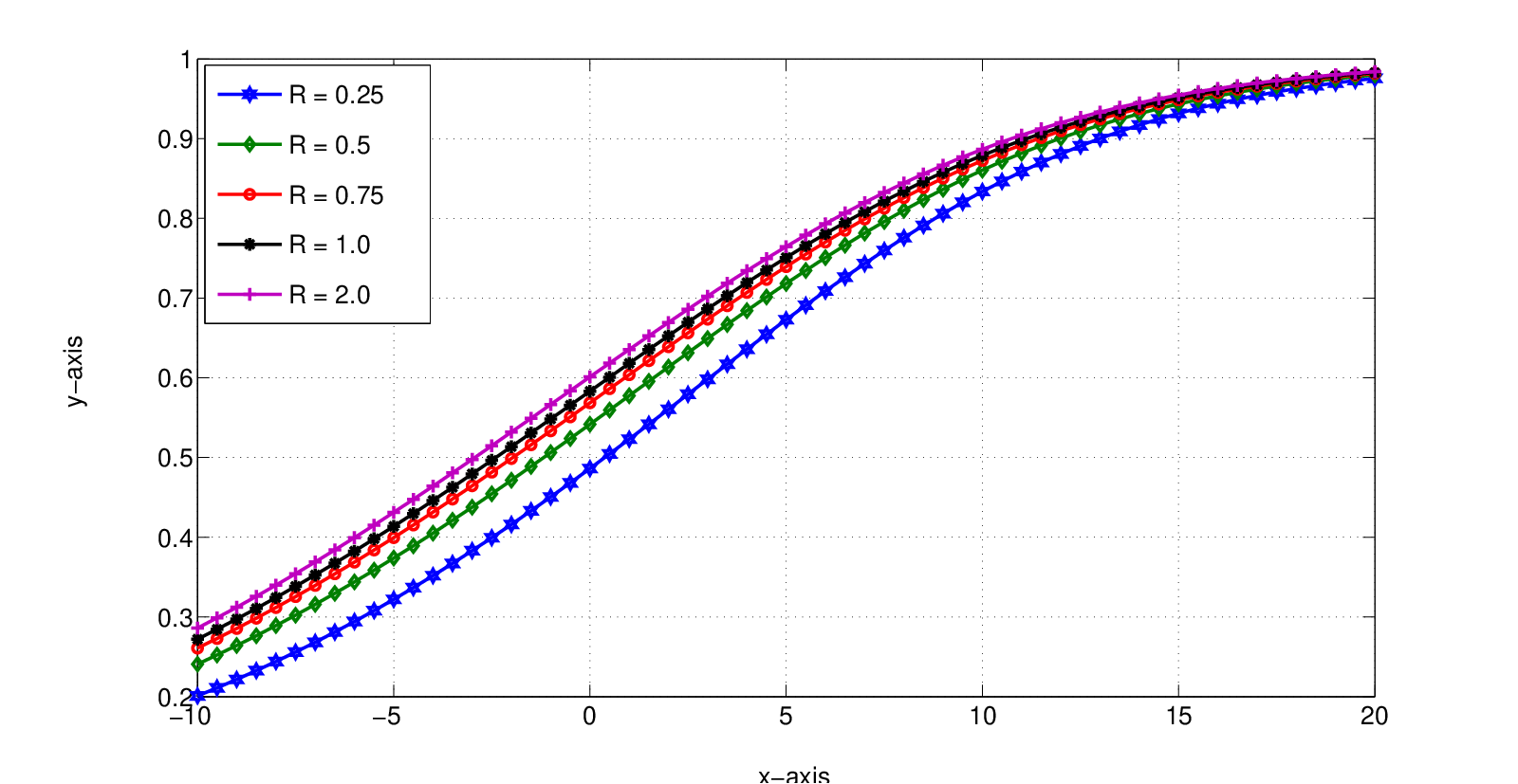
and $\theta=\pi-\sin^{-1}2^{-R}$. Shown in Fig. 2 is a plot of $E_{as}(R,S)/E(S)$ as a function of $S$, repeated for various $R$. As can be seen from the plot $E_{as}(R,S)$ is always smaller than $E(S)$ for any $R$ and $S$, thus showing that the bound obtained in Theorem 1 is tighter than the one given by (15). The current bound is also seen to be better when the SNR $S$ is not very high.

References

• [1] U. Niesen, C. Fragouli, and D. Tuninetti, “On capacity of line networks,” IEEE Trans. Inform. Theory, vol. 53, no. 11, pp. 4039–4058, Nov. 2007.
• [2] R. Subramanian, “The relation between block length and reliability for a cascade of awgn links,” Proceedings of the 2012 International Zurich Seminar on Communications (IZS), pp. 71–74, Feb. 29 – Mar. 2, 2012.
• [3] Claude E. Shannon, “Probability of error for optimal codes in a gaussian channel,” Claude Elwood Shannon: Collected Papers, pp. 279–324, 1993.
• [4] Atsuyuki Okabe, Barry Boots, and Kokichi Sugihara, Spatial tessellations: concepts and applications of Voronoi diagrams, chapter 3, John Wiley & Sons, Inc., New York, NY, USA, 1992.
Appendix A The Farthest-point Voronoi Tessellation for Points on a Sphere
Lemma 6
Given any M,N∈ℕM,N\in\mathds{N}, the non-empty cells in the farthest-point Voronoi tessellation of ℝN\mathds{R}^{N} w.r.t. any set of MM points on an NN-sphere of radius A>0A>0 are all semi-infinite pyramids.
Proof:
Consider the farthest-point Voronoi tessellation of ℝN\mathds{R}^{N} w.r.t. a code 𝒞=(𝐜1,…,𝐜M)​s.t.​‖𝐜i‖2=A2,1≤i≤M\mathscr{C}=\left(\mathbf{c}_{1},\ldots,\mathbf{c}_{M}\right)\text{s.t.}\|\mathbf{c}_{i}\|^{2}=A^{2},1\leq i\leq M. Consider any 𝐱∈ℝN\mathbf{x}\in\mathds{R}^{N} and assume without loss of generality that it is contained in ℛ1∗\mathcal{R}^{*}_{1}, the farthest-point Voronoi cell for 𝐜1′\mathbf{c}^{\prime}_{1}. In that case, we have for all ii s.t. 1≤i≤M1\leq i\leq M,
‖𝐜1−𝐱‖2\displaystyle\|\mathbf{c}_{1}-\mathbf{x}\|^{2} ≥\displaystyle\geq ‖𝐜i−𝐱‖2\displaystyle\|\mathbf{c}_{i}-\mathbf{x}\|^{2}
⇒‖𝐜1‖2+‖𝐱‖2−2​⟨𝐜1,𝐱⟩\displaystyle\Rightarrow\|\mathbf{c}_{1}\|^{2}+\|\mathbf{x}\|^{2}-2\langle\mathbf{c}_{1},\mathbf{x}\rangle ≥\displaystyle\geq ‖𝐜i‖2+‖𝐱‖2−2​⟨𝐜i,𝐱⟩\displaystyle\|\mathbf{c}_{i}\|^{2}+\|\mathbf{x}\|^{2}-2\langle\mathbf{c}_{i},\mathbf{x}\rangle
⇒−⟨𝐜1,𝐱⟩\displaystyle\Rightarrow-\langle\mathbf{c}_{1},\mathbf{x}\rangle ≥\displaystyle\geq −⟨𝐜i,𝐱⟩.\displaystyle-\langle\mathbf{c}_{i},\mathbf{x}\rangle. (16)
Consider any α≥0\alpha\geq 0. We claim that α​𝐱\alpha\mathbf{x} is also contained in ℛ1∗\mathcal{R}^{*}_{1}. This can be shown to be true by applying (16) to the expansion of ‖𝐜1−α​𝐱‖2\|\mathbf{c}_{1}-\alpha\mathbf{x}\|^{2}:
‖𝐜1−α​𝐱‖2\displaystyle\|\mathbf{c}_{1}-\alpha\mathbf{x}\|^{2} =\displaystyle= ‖𝐜1‖2+α2​‖𝐱‖2−2​α​⟨𝐜1,𝐱⟩\displaystyle\|\mathbf{c}_{1}\|^{2}+\alpha^{2}\|\mathbf{x}\|^{2}-2\alpha\langle\mathbf{c}_{1},\mathbf{x}\rangle
≥\displaystyle\geq ‖𝐜i‖2+α2​‖𝐱‖2−2​α​⟨𝐜i,𝐱⟩\displaystyle\|\mathbf{c}_{i}\|^{2}+\alpha^{2}\|\mathbf{x}\|^{2}-2\alpha\langle\mathbf{c}_{i},\mathbf{x}\rangle
=\displaystyle= ‖𝐜i−α​𝐱‖2,\displaystyle\|\mathbf{c}_{i}-\alpha\mathbf{x}\|^{2},
for all ii s.t. 1≤i≤M1\leq i\leq M. Hence, α​𝐱\alpha\mathbf{x} is also contained in ℛ1∗\mathcal{R}^{*}_{1}. Generalizing this, we have shown that any non-empty Voronoi cell that contains a point 𝐱\mathbf{x} also contains the point α​𝐱\alpha\mathbf{x} for any α≥0\alpha\geq 0. Such a region is a semi-infinite pyramid by definition. ∎
Appendix B Proof of the claim in Lemma 5
Consider the N−1N-1 dimensional cross-section of the pyramid ℛk∗\mathcal{R}^{*}_{k} cut out by a sphere of radius RR centered at the origin. This will be an arbitrary spherical polygon. The cross-section of the cone 𝒞k∗\mathcal{C}^{*}_{k} by the same sphere will be a spherical cap with its center at −𝐜k-\mathbf{c}_{k}. The axis of the cone cuts through the spherical cap at its center. The non-overlapping regions of such a spherical cap and a polygon are illustrated in Fig. 3. Since the both the cross sections have the same surface area RN​ΩkR^{N}\Omega_{k}, the surface areas of the non-overlapping parts of both the cross-sections (indicated as A1A_{1} and A2A_{2} and by two different shadings in Fig. 3) are equal. Now, every point in the shaded region A1A_{1} on the polygon is nearer to 𝐜k\mathbf{c}_{k} than any point in A2A_{2} is to 𝐜k\mathbf{c}_{k}. This is because the former lies outside the spherical cap centered at −𝐜k-\mathbf{c}_{k} while the latter is inside the same. This in turn implies that the angle θ2∈[0,π]\theta_{2}\in[0,\pi] between the axis of the cone and the line joining any point 𝐲2\mathbf{y}_{2} on A2A_{2} and the origin is smaller than the angle θ1∈[0,π]\theta_{1}\in[0,\pi] between the axis and the line joining any point 𝐲1\mathbf{y}_{1} on A1A_{1} and the origin, as shown in the right hand side of Fig. 3. This in turn implies that 𝐲1\mathbf{y}_{1} is closer to 𝐜k\mathbf{c}_{k} than 𝐲2\mathbf{y}_{2} is to 𝐜k\mathbf{c}_{k}, as shown below:
‖𝐜k−𝐲1‖2\displaystyle\|\mathbf{c}_{k}-\mathbf{y}_{1}\|^{2} =\displaystyle= NP0+R2+2RN​P0cosθ1\displaystyle NP_{0}+R^{2}+2R\sqrt{NP_{0}}\cos{\theta_{1}}
≤\displaystyle\leq NP0+R2+2RN​P0cosθ2\displaystyle NP_{0}+R^{2}+2R\sqrt{NP_{0}}\cos{\theta_{2}}
=\displaystyle= ‖𝐜k−𝐲2‖2.\displaystyle\|\mathbf{c}_{k}-\mathbf{y}_{2}\|^{2}.
This in turn means that the integral of the density function of the Gaussian noise vector with center at 𝐜k\mathbf{c}_{k} over the volume ℛk∗\mathcal{R}^{*}_{k} is greater than the integral over the volume 𝒞k∗\mathcal{C}^{*}_{k}. The former is the probability of the event E1E_{1} and the latter is the probability of the event E2E_{2}.
Refer to caption
Fig. 3: Illustration of the fact that the non-overlapping portion of the pyramidal cross-section is nearer to the original codeword than the non-overlapping portion of the conical cross section.
Appendix C Asymptotic exponential decay of the 𝒬\mathcal{Q} function with NN
Though it is hard to express 𝒬\mathcal{Q} in terms of elementary functions, it is easy to obtain asymptotic approximations when the block length NN is very large. The idea is to use Shannon’s computation of the sphere-packing exponent. Shannon derives a bound on 𝒬(.)\mathcal{Q}\left(.\right) as a function of the cone angle θ∈[0,π]\theta\in[0,\pi] instead of the solid angle Ω\Omega since this makes asymptotic analysis easier. This results in a bound for 𝒬(.)\mathcal{Q}\left(.\right) that decays exponentially in NN, with the exponent being
EL​(θ)=P02​σ02−12​P0σ02​G​cos⁡θ−log⁡(G​sin⁡θ),E_{L}\left(\theta\right)=\frac{P_{0}}{2\sigma_{0}^{2}}-\frac{1}{2}\sqrt{\frac{P_{0}}{\sigma_{0}^{2}}}G\cos\theta-\log\left(G\sin\theta\right),
where
G=12​(P0σ02​cos⁡θ+4+P0σ02​cos2⁡θ).G=\frac{1}{2}\left(\sqrt{\frac{P_{0}}{\sigma_{0}^{2}}}\cos\theta+\sqrt{4+\frac{P_{0}}{\sigma_{0}^{2}}\cos^{2}\theta}\right).
The bound on 𝒬(.)\mathcal{Q}\left(.\right) for a given Ω\Omega can then be evaluated numerically or by any other means, since there is a one-to-one correspondence between the cone angle θ0\theta_{0} and the solid angle Ω\Omega (see Fig. 4):
Ω⁡(θ0)=(N−1)​πN−12Γ⁡(N+12)​∫0θ0(sin⁡θ0)N−2​d​θ0.\Omega\left(\theta_{0}\right)=\frac{(N-1)\pi^{\frac{N-1}{2}}}{\Gamma\left(\frac{N+1}{2}\right)}\int_{0}^{\theta_{0}}\left(\sin\theta_{0}\right)^{N-2}\mathrm{d}\theta_{0}.
The particular case of interest in [3] is 𝒬⁡(1M​Ω0,N,P0σ02)\mathcal{Q}\left(\frac{1}{M}\Omega_{0},N,\frac{P_{0}}{\sigma_{0}^{2}}\right), which corresponds to the cone angle θ=sin−1⁡2−R\theta=\sin^{-1}2^{-R} and the sphere-packing lower bound is obtained thus (see pages 620 and 625 in [3]). Our bound involves 𝒬⁡(M−1M​Ω0,N,P0σ02)\mathcal{Q}\left(\frac{M-1}{M}\Omega_{0},N,\frac{P_{0}}{\sigma_{0}^{2}}\right) instead, and hence we will have to evaluate the exponent EL​(θ)E_{L}\left(\theta\right) with θ=π−sin−1⁡2−R\theta=\pi-\sin^{-1}2^{-R} instead, giving us the following result:
Fig. 4: Relation between solid angle and cone angle.
ℐ⁡(W,W^n)⪅(1−e−N​Ea​s​(R,P0/σ02))n,\displaystyle\mathcal{I}\left(W;\hat{W}_{n}\right)\lessapprox\left(1-e^{-NE_{as}\left(R,P_{0}/\sigma_{0}^{2}\right)}\right)^{n}, (17)
where Ea​s​(R,S)E_{as}\left(R,S\right) is as shown in (18).
Ea​s​(R,S)\displaystyle E_{as}\left(R,S\right) =\displaystyle= S22​R+2​((22​R+1)+(22​R−1)​1+22​R+2(22​R−1)​S)\displaystyle\frac{S}{2^{2R+2}}\left((2^{2R}+1)+(2^{2R}-1)\sqrt{1+\frac{2^{2R+2}}{\left(2^{2R}-1\right)S}}\right) (18)
+12​log⁡[22​R+S2​(22​R−1)​(1+22​R+2(22​R−1)​S+1)]−R​log⁡2.\displaystyle\ \ \ \ \ +\frac{1}{2}\log\left[2^{2R}+\frac{S}{2}(2^{2R}-1)\left(\sqrt{1+\frac{2^{2R+2}}{\left(2^{2R}-1\right)S}}+1\right)\right]-R\log 2.