跳到论文正文
W Papers独立论文阅读器 arXiv:1301.6252 论文正文 计算阅读时间 · 0%
引用这篇论文根据当前论文元数据生成,正式投稿前建议核对。


License: arXiv.org perpetual non-exclusive license
arXiv:1301.6252v3 [q-fin.PR] 11 Aug 2016

Option pricing with linear market impact and non-linear Black-Scholes Equations

Grégoire LOEPER Address: Monash University, School of Mathematical Sciences Email address: gregoire.loeper@monash.edu
Date: August 24, 2026
Abstract.

We consider a model of linear market impact, and address the problem of replicating a contingent claim in this framework. We derive a non-linear Black-Scholes Equation that provides an exact replication strategy.

This equation is fully non-linear and singular, but we show that it is well posed, and we prove existence of smooth solutions for a large class of final payoffs, both for constant and local volatility. To obtain regularity of the solutions, we develop an original method based on Legendre transforms.

The close connections with the problem of hedging with gamma constraints [29], [31], [25], with the problem of hedging under liquidity costs [9] are discussed. The optimal strategy and associated diffusion are related with the second order target problems of [32], and with the solutions of optimal transport problems by diffusions of [33].

We also derive a modified Black-Scholes formula valid for asymptotically small impact parameter, and finally provide numerical simulations as an illustration.

1. Introduction

This paper is about the derivation and mathematical analysis of a pricing model that takes into account the market impact of the option’s hedger, i.e. the feedback mechanism between the option’s delta-hedging and the price dynamics. We will throughout the paper assume a linear market impact: each order to buy NN stocks impacts the stock price by λ​N​S2\lambda NS^{2} (λ≥0\lambda\geq 0). This scaling, that will be discussed hereafter, means that the impact in terms of relative price move depends on the amount of stock traded expressed in currency, hence λ\lambda is homogeneous to the inverse of the currency i.e. percents per dollar.

(1) Order to buy N stocks⟹S→S⁡(1+λ​N​S).\displaystyle\hbox{Order to buy N stocks}\implies S\to S(1+\lambda NS).

We will examine several situations where λ\lambda is either constant, or can be also a function of the solution itself.

The literature devoted to the study of the market impact itself is quite vast, and it is more frequent to find an impact that varies as a power law of the size of the trade (see for example [2]). Although our linear approach is clearly not the most realistic in terms of market microstructure, it has the advantage of avoiding arbitrage opportunities, as well as not being sensitive to the hedging frequency: in a non-linear model, splitting an order in half and repeating it twice would not yield the same result, a situation that we want to avoid here, as we aim at deriving a time continuous formulation.

In addition we assume that the market impact is permanent: there is no relaxation following the immediate impact, where the price goes back partially to its pre-trade value. The case with relaxation has been studied in a companion paper [1].

1.1. Order book modeling

From an order book perspective, our market impact model consists in assuming an order book with continuous positive density around the mid-price, and where following a market-order starting at price SS (say a buy order for example), where liquidity has been consumed up to S+δ​SS+\delta S, the new mid-price becomes S+δ​SS+\delta S, and the liquidity removed between SS and S+δ​SS+\delta S is instantaneously refilled with buy orders (or sell orders if the price had moved down after a sell order). Clearly this model is a great simplification of what is actually observed in real markets (see [34] for instance), but as we will show this simple approach is enough to obtain a non-trivial modification of the usual Black-Scholes equation. More precisely: Assume a static order book, parametrized by a mid price S¯\bar{S} and a supply intensity μ⁡(t,s)\mu(t,s) in the following way: the number of stocks available for purchase between SS and S+d​SS+dS equals to μ⁡(t,S)​d​S\mu(t,S)dS.

We assume that the (local) liquidity (expressed in currency) available between S¯\bar{S} and S¯​(1+ε)\bar{S}(1+\varepsilon) equals L⁡(t,S¯)​ε+o⁡(ε)L(t,\bar{S})\varepsilon+o(\varepsilon). Simple calculations show that the scaling (1) implies that L⁡(t,S)L(t,S) is actually constant, which explains our choice, as we believe that the quantity LL is the good measure of a stock’s liquidity. Then independently of this choice, when spending an amount AA (expressed in currency) in stocks, the order book will be consumed up to S¯​(1+ϵ)\bar{S}(1+\epsilon) given by

A=∫S¯S¯​(1+ε)μ⁡(t,s)​s​𝑑s,A=\int_{\bar{S}}^{\bar{S}(1+\varepsilon)}\mu(t,s)sds,

while the number of stocks purchased will be

N=∫S¯S¯​(1+ε)μ⁡(t,s)​𝑑s.N=\int_{\bar{S}}^{\bar{S}(1+\varepsilon)}\mu(t,s)ds.

One sees right away that, at the leading order, the average price of execution is S¯​(1+12​ε)\bar{S}(1+\frac{1}{2}\varepsilon). In a subsequent study [1], the authors consider an immediate relaxation of the price after the liquidity is consumed, hence the liquidity of the order book is rebuilt around S¯​(1+γ​ε)\bar{S}(1+\gamma\varepsilon) for a certain relaxation factor γ∈[0,1]\gamma\in[0,1]. We will only adress here the case γ=1\gamma=1. The choice γ=0\gamma=0 is the one that has been studied by Cetin, Soner and Touzi in [9]: no permanent market impact, but liquidity costs.

1.2. Motivations and links with previous works

In terms of concrete applications, the problem of derivatives pricing with market impact arises when the delta hedging of the option implies a volume of transactions on the underlying asset that is non-negligible compared to the average daily volume traded. For example, a well observed effect known as stock pinning arises when the hedger is long of the (convex) option for a large notional, and one observes then a decrease of realized volatility if the underlying ends near the strike at maturity. In financial terms, the hedger of the option makes a loss if the volatility realizes below its implied value. This stylized fact can be recovered by our pricing equation. Conversely, when selling a convex option for a large notional, a common market practice on derivatives desks is to super-replicate the option by the cheapest payoff satisfying a constraint of gamma (the second derivative of the option), the gamma max being adjusted to the liquidity available on the option’s underlying. Hence there are two issues arising here:

  • -

    Be able to control a priori the trading volume due to delta-hedging: this approach has been studied in depth in the works by Soner and Touzi [31] and Cheridito, Soner and Touzi [25] that deal with the problem of heging with gamma-constraints.

  • -

    Quantify the liquidity costs induced by the delta-hedging, and incorporate them in the option’s price, this has been studied by Cetin, Jarrow and Protter in [8] and by Cetin, Soner and Touzi in [9]. However these works consider only liquidity costs, and not the effect of permanent market impact.

Our approach addresses those two issues: first, via the market impact mechanism, it induces a constraint on the gamma when selling a convex payoff, and it constraints the theta (the time derivative of the option) when selling a concave payoff. Thus it recovers two important stylized facts of the gamma constraint approach, moreover it incorporates liquidity costs in the price. It can be noted that the parabolic operator that we obtain through market impact lies somehow between the gamma-constraint operator of [29] and the liquidity costs operator of [9].

A formal argument shows that, playing on the dependency of the market impact parameter with the solution, one can recover exactly the gamma constraint pricing equation of Cheridito Soner Touzi [25], or the liquidity cost equation of Cetin, Soner and Touzi in [9]. This can be seen as closely related to the work of Serfaty and Kohn [20] that recover non-linear heat equations by stationary games approach. From a financial modelling perspective, this would amount to assume a supply curve for the price of gamma-hedging.

Concerning the mathematical techniques, as opposed to [25], [9], [31], [5], [6], we adress the problem of finding exact replication strategies, while the aforementioned work deal with stochastic target problems: find the cheapest trading strategy that super-replicates the final payoff. The solutions of these two problems coïncide in general, but may differ in some degenerate cases (see [30], [1]). Apart from introducing the linear market impact model (which has then led to the subsequent studies [5], [6], [1]), the main contribution of this paper is a complete study of a fully non linear parabolic equation associated to a new class of stochastic control problems (see Theorem 5.5). We will also prove a representation formula that gives some qualitative informations about the modified dynamics. Those two results are then used to derive rigorously an asymptotic expansion of the solution for small market impact, leading to a modified Black-Scholes-Legendre formula, as well as a simple and efficient way of computing the market impact effect.

We believe that the techniques used toward obtaining these results are original and of independent interest. As will be discussed hereafter, these results can be seen as related to regularity results concerning porous media equations (see the book of Vazquez [36] for a complete reference), in particular in the case of Fast Diffusion Equations, as well as the papers by Crandall and Pierre [13], [11] about interior regularity for non-linear diffusions.

The stochastic target problem associated to our model has been studied in two companion papers [5], [6], where it is shown that the exact replication strategy is actually the optimal solution for the stochastic target problem. To make a connection between the two results, it is important to notice that through stochastic control techniques, one is able to derive a viscosity formulation of the value function. It is only when this function has enough regularity that one can deduce the optimal strategy from the value function, hence the importance of the question of regularity.

Finally we mention the references ([21], [26], [28], [14], [15], [26]) that also address the problem of option hedging in non-perfect markets with different approaches, leading to different mathematical techniques.

1.3. The pricing equation

As we will see, assuming no interest rates and dividends, the pricing equation that we obtain can be put under the form

(2) ∂tu+12​σ2​s2​∂s​su1−λ​s2​∂s​su=0,\displaystyle\partial_{t}u+\frac{1}{2}\sigma^{2}\frac{s^{2}\partial_{ss}u}{1-\lambda s^{2}\partial_{ss}u}=0,

which reads also

σ22​∂tu+1s2​∂s​su=λ,\displaystyle\frac{\sigma^{2}}{2\partial_{t}u}+\frac{1}{s^{2}\partial_{ss}u}=\lambda,

where λ\lambda can be either constant or dependent of the solution as λ⁡(s2​∂s​su)\lambda(s^{2}\partial_{ss}u). In this case we obtain a wide class of fully non-linear Black Scholes equations of the form

∂tu+12​σ2​F​(s2​∂s​su)=0.\displaystyle\partial_{t}u+\frac{1}{2}\sigma^{2}F(s^{2}\partial_{ss}u)=0.

As will be shown, one can derive any parabolic equation of this form through an ad-hoc choice of λ\lambda, as long as F⁡(γ)≥γF(\gamma)\geq\gamma and F⁡(0)=0F(0)=0.

The case of equation (2) is quite challenging for the mathematical perspective: the operator ∂s​su→F⁡(s2​∂s​su)\partial_{ss}u\to F(s^{2}\partial_{ss}u) is not uniformly elliptic (when ∂s​su\partial_{ss}u goes to −∞-\infty), and is singular (when s2​∂s​sus^{2}\partial_{ss}u goes to λ−1\lambda^{-1}). Standard theory does not apply right away, and an ad-hoc regularity theory must be developed. Still, we will be able to show interior (i.e. not relying on a smooth terminal payoff) regularity of solutions for constant λ\lambda and boundary regularity (i.e. assuming a good terminal condition) for non-constant λ\lambda.

Let us rewrite equation (2) as follows:

∂tu+12​σ2​F​(s2​∂s​su)=0,\displaystyle\partial_{t}u+\frac{1}{2}\sigma^{2}F(s^{2}\partial_{ss}u)=0,
F⁡(γ)=γ1−λ​γ=1λ​(−1+11−λ​γ).\displaystyle F(\gamma)=\frac{\gamma}{1-\lambda\gamma}=\frac{1}{\lambda}(-1+\frac{1}{1-\lambda\gamma}).

The link with non linear diffusions appears when one differentiates twice the equation: assuming σ\sigma constant one then obtains for β=1−λ​s2​∂s​su\beta=1-\lambda s^{2}\partial_{ss}u

∂tβ−σ2​s22​∂s​s(1β)=0,\displaystyle\partial_{t}\beta-\frac{\sigma^{2}s^{2}}{2}\partial_{ss}\left(\frac{1}{\beta}\right)=0,

which can be seen as a lognormal version of the Fast Diffusion Equation (see [36])

∂tu−Δ⁡(1u)=0.\displaystyle\partial_{t}u-\Delta\left(\frac{1}{u}\right)=0.

1.4. Second order target problems and optimal transport by diffusions

There is also a clear connection between this work and the work by Soner and Touzi and Zhang [32] about dual formulation of second order target problems, and also with the problems of optimal transport by controlled martingales studied in [33]. Indeed observe that the elliptic operator F⁡(γ)F(\gamma) in (2) is convex, and then applying the reasoning of [32] based on the Legendre transform representation of FF, one can show formally that a solution to (2) will also be solution of the following variational problem:

(3) u(t,s)=supa∈𝒜T{𝔼{Φ(ST)−12​λ∫tT(at′1/2−σ(t′,St′a))2dt′}.\displaystyle u(t,s)=\sup_{a\in{\mathcal{A}_{T}}}\Big\{\mathbb{E}\{\Phi(S_{T})-\frac{1}{2\lambda}\int_{t}^{T}(a_{t^{\prime}}^{1/2}-\sigma(t^{\prime},S^{a}_{t^{\prime}}))^{2}dt^{\prime}\Big\}.

where SaS^{a} starts from ss at time tt and follows d​Sra=ar1/2​Sra​d​WrdS^{a}_{r}=a^{1/2}_{r}S^{a}_{r}dW_{r}, WrW_{r} is a Brownian motion, 𝒜T{\mathcal{A}_{T}} is the set of all bounded positive adapted processes on [t,T][t,T], and σ⁡(t,s)\sigma(t,s) is given and positive.

This can be seen as a stochastic version of Hopf-Lax formula,

(4) u⁡(t,s)=supγ∈C1​([0,T]),γ⁡(t)=s{Φ⁡(γ⁡(T))−12​λ​∫tTH⁡(∂tγ⁡(t′))​d​t′},\displaystyle u(t,s)=\sup_{\gamma\in{C^{1}([0,T])},\gamma(t)=s}\Big\{\Phi(\gamma(T))-\frac{1}{2\lambda}\int_{t}^{T}H(\partial_{t}\gamma(t^{\prime}))dt^{\prime}\Big\},

see [4], which is a representation formula for solutions to

∂tu+H∗​(Dx​u)=0,\displaystyle\partial_{t}u+H^{*}(D_{x}u)=0,

where H∗H^{*} is the Legendre transform of HH. The fact that, in general, the solution of a variational problem like (3) is indeed the viscosity solution of an associated parabolic equation (which here would be 2) has been studied in [32]. In this particular case we will be able to actually characterize the optimal a^\hat{a} in (3), and show that the optimal diffusion Sa^S^{\hat{a}} is a martingale up to time TT under mild conditions, which allow a^\hat{a} to be unbounded.

Then, still reasoning formally, Sa^S^{\hat{a}} transports its initial distribution on its final distribution minimizing the transport cost

𝔼⁡(12​∫0T(at1/2−σ⁡(t,St))2​𝑑t),\displaystyle\mathbb{E}\left(\frac{1}{2}\int_{0}^{T}(a_{t}^{1/2}-\sigma(t,S_{t}))^{2}dt\right),

which is a particular case of the problem studied in [33]. More generally the link between the variational problem (3) and optimal transport arises through the use of Kantorovitch duality, see [17], [18], [7] and also [37] for an overview on optimal transport, and also [24] for further extensions to non-linear variational problems.

The regularity results that we obtain here will provide the regularity of the optimizers in the aforementioned problems.

1.5. Organization of the paper

The rest of the paper is organized as follows: in the next section (Section 2) we provide a heuristic derivation of the pricing equation, and discuss its practical relevance for financial modelling.

Section 3 gives the time continuous formulation of the problem as a system of stochastic differential equations, and shows that the pricing equation (2) actually leads to an exact replication strategy when it admits a smooth solution, see Theorem 3.2.

Section 4 establishes the connection between the solution of (2) and the problem (3), and discusses also the link with optimal transport and robust hedging.

Section 5 contains the regularity results for the pde (2). Theorems 5.5, 5.7 and 5.13, contain the main a priori estimates for solutions to (2), that hold under mild conditions on the final payoff. These results lead then to the existence, regularity and uniqueness of the solutions to (2): Theorem 5.16.

Section 6 establishes representation formulas for the solution: Theorems 6.7, 6.3 and 6.8. These representation formulas are a probabilistic counterpart to the pde (2), and give qualitative insight about the solution, and establish further results concerning the optimizers of the problem (3).

In section 7 we derive a first order expansion of the solution for small market impact (λ\lambda). This leads also to modified Black-Scholes-Legendre formula (see formulas (100, 102, 103)), which is easily computed by analytic formulas or standard Monte-Carlo simulations. It should formally be also valid in the liquidity costs case of [9].

Section 8 illustrates the paper with a numerical solution of the pde.

1.6. Acknowledgements

This paper has been in gestation for a long time, its motivation originally appeared while the author was a member of the Quantitative Research team at BNP Paribas Capital Markets, and I thank my colleagues there for stimulating discussions. Part of this work has also been done under the hospitality of the Chair of Quantitative Finance at the Ecole Centrale de Paris, and I thank in particular Frédéric Abergel. I also thank Bruno Bouchard, Nizar Touzi, Juan Vazquez, Fernando Quiros, and Fima Klebaner for enlightening discussions.

2. Heuristics

We assume that we have sold an option whose value is u⁡(t,s)u(t,s), and greeks are as usual

Δ\displaystyle\Delta =\displaystyle= ∂su,\displaystyle\partial_{s}u,
Γ\displaystyle\Gamma =\displaystyle= ∂sΔ,\displaystyle\partial_{s}\Delta,
Θ\displaystyle\Theta =\displaystyle= ∂tu.\displaystyle\partial_{t}u.

We also introduce the Gamma in currency, i.e.

(5) γ=Γ​S2.\displaystyle\gamma=\Gamma S^{2}.

The strategy that we use is the following: we assume a priori that there exists an exact replication strategy, that consists in holding Δ=∂su\Delta=\partial_{s}u stocks. We compute the equation that must be followed by uu, and the modified dynamics that this strategy implies. We then check that this strategy allows indeed to perfectly replicate the final claim.

Starting from a delta-hedged portfolio, assume that the stock price SS moves by d​SdS. We will assume that this initial move of d​SdS is given as is usual by

d​S=S​σ​d​Wt,\displaystyle dS=S\sigma dW_{t},

where WtW_{t} is a standard Brownian motion, and d​WtdW_{t} its increment between tt and t+d​tt+dt (those objects will be introduced more formally later on). A ‘naive’ hedge would be to buy Γ​d​S\Gamma dS stocks, but as this order will impact the market, the portfolio will not end up delta-hedged. Assume instead a hedge adjustment of μ​Γ​d​S\mu\Gamma dS stocks, and let us find μ\mu such that spot ends up at a final value S+μ​d​SS+\mu dS. Using (1), we write that

Safter re-hedging−Sbefore re-hedging=λ​S2​Number of stocks bought to re-hedge,\displaystyle S_{\text{after re-hedging}}-S_{\text{before re-hedging}}=\lambda S^{2}\;\text{Number of stocks bought to re-hedge},

and this yields

μ​d​S−d​S=λ⁡[Δ⁡(S+μ​d​S)−Δ⁡(S)]​S2.\displaystyle\mu dS-dS=\lambda[\Delta(S+\mu dS)-\Delta(S)]S^{2}.

This identity expresses the fact that the number of titles bought is Δ⁡(S+μ​d​S)−Δ⁡(S)\Delta(S+\mu dS)-\Delta(S), hence that the portfolio is delta-hedged at the end of the trade. Performing a first order Taylor expansion leads to

(6) Γ​μ​d​S​λ​S2=(μ−1)​d​S+o⁡(d​S),\displaystyle\Gamma\mu dS\lambda S^{2}=(\mu-1)dS+o(dS),

which yields

(7) μ=11−λ​γ.\displaystyle\mu=\frac{1}{1-\lambda\gamma}.

Remember that γ\gamma is computed with respect to the option the portfolio is short of, hence γ>0\gamma>0 when one sells a call for example. Assuming that λ​γ<1\lambda\gamma<1 (to be discussed later), one sees that μ>1\mu>1: as expected the hedger increases the volatility by buying when the spot rises, and selling when it goes down.

One can also reach the conclusion (7) by following an iterative hedging strategy: after the initial move S→S+d​SS\to S+dS, the hedge is adjusted ”naively” by Γ​d​S\Gamma dS stocks, which then impacts the price by d​S2=λ​S2​Γ​d​SdS_{2}=\lambda S^{2}\Gamma dS. A second re-hedge of Γ​d​S2\Gamma dS_{2}is done, which in turn impacts the price and so forth. The final spot move is thus the sum of the geometric sequence

d​S​(1+λ​S2​Γ+(λ​S2​Γ)2+…)=d​S1−λ​γ.\displaystyle dS(1+\lambda S^{2}\Gamma+(\lambda S^{2}\Gamma)^{2}+...)=\frac{dS}{1-\lambda\gamma}.

One sees right away that in this sequence, the critical point is reached when the ”first” re-hedge (i.e. buying Γ​d​S\Gamma dS stocks after the initial move of d​SdS) doubles the initial move: the sum will not converge. This situation will be discussed hereafter.

Then the value QQ of the portfolio containing -1 option + Δ\Delta stocks at the beginning of time tt, and Δ⁡(S+μ​d​S)\Delta(S+\mu dS) stocks at time t+d​tt+dt evolves as

d​Q=u⁡(t,S)−u⁡(t+d​t,S+μ​d​S)+Δ​μ​d​S+ℛ\displaystyle dQ=u(t,S)-u(t+dt,S+\mu dS)+\Delta\mu dS+\mathcal{R}

and ℛ\mathcal{R} is the profit realized during the re-hedging. In a perfect frictionless market, this term is zero, as one buys d​Δd\Delta stocks at a price S+d​SS+dS, and the ”post-re-hedge” value of the stocks is S+d​SS+dS. To compute ℛ{\mathcal{R}} we recall that

(8) Immediate impact of an order to buy N stocks ⟹\displaystyle\implies S→S⁡(1+λ​N​S),\displaystyle S\to S(1+\lambda NS),
(9) Average execution price =\displaystyle= S⁡(1+12​λ​N​S).\displaystyle S(1+\frac{1}{2}\lambda NS).

The computation of ℛ\mathcal{R} then yields

ℛ\displaystyle\mathcal{R} =\displaystyle= N⁡(Final price of the stocks bought−Average execution price)\displaystyle N\Big(\text{Final price of the stocks bought}-\text{Average execution price}\Big)
=\displaystyle= N⁡(S⁡(1+λ​N​S)−S⁡(1+12​λ​N​S))\displaystyle N\Big(S(1+\lambda NS)-S(1+\frac{1}{2}\lambda NS)\Big)
=\displaystyle= 12​λ​N2​S2,\displaystyle\frac{1}{2}\lambda N^{2}S^{2},

with N=Γ​μ​d​SN=\Gamma\mu dS. Finally if VV is the the value of the hedger’s trading strategy, and setting d​S~=μ​d​Sd\tilde{S}=\mu dS, one obtains:

(10) d​V=Δ​d​S~+12​λ​S2​(Γ​d​S~)2.\displaystyle dV=\Delta d\tilde{S}+\frac{1}{2}\lambda S^{2}(\Gamma d\tilde{S})^{2}.

2.0.1. The pricing equation

We now assume that the option is sold at its fair price, hence d​Q=0dQ=0 at first order in time. Then we have as SS moves to S+μ​d​SS+\mu dS,

d​u=∂tu​d​t+∂su​μ​d​S+12​∂s​su​(μ​d​S)2+o⁡(d​t),\displaystyle du=\partial_{t}udt+\partial_{s}u\mu dS+\frac{1}{2}\partial_{ss}u(\mu dS)^{2}+o(dt),

and we thus get

∂tu​d​t+(μ​d​S)2/2​[∂s​su−λ​(∂s​su)2​S2]=o⁡(d​t),\displaystyle\partial_{t}udt+(\mu dS)^{2}/2\left[\partial_{ss}u-\lambda(\partial_{ss}u)^{2}S^{2}\right]=o(dt),

with μ\mu defined by (7). We recall now that the initial move of SS i.e. d​SdS in our notations, is driven by a geometric Brownian motion, as in the Black-Scholes model, so d​S=S​σ​d​WdS=S\sigma dW. Then one can following Itô’s formula replace (d​S)2(dS)^{2} by σ2​S2​d​t\sigma^{2}S^{2}dt in the previous Taylor expansion, and this simplifies into

(11) ∂tu+12​σ2​F​(γ)=0,\displaystyle\partial_{t}u+\frac{1}{2}\sigma^{2}F(\gamma)=0,
(12) F⁡(γ)=γ1−λ​γ,\displaystyle F(\gamma)=\frac{\gamma}{1-\lambda\gamma},
(13) γ=s2​∂s​su.\displaystyle\gamma=s^{2}\partial_{ss}u.

Remark. Note that if we change assumption (9) in

(14) Average execution price =\displaystyle= S⁡(1+λ​N​S),\displaystyle S(1+\lambda NS),

then we get the equation

∂tu+12​σ2​γ(1−λ​γ)2=0,\displaystyle\partial_{t}u+\frac{1}{2}\sigma^{2}\frac{\gamma}{(1-\lambda\gamma)^{2}}=0,

as found in [23]. This equation is not parabolic however.

When λ→0\lambda\to 0, we we recover the standard Black-Scholes equation. This equation clearly poses problems when 1−λ​γ1-\lambda\gamma goes to 0, and even becomes negative. This case arises when one has sold a convex payoff (γ>0\gamma>0) and an initial move of d​SdS would be more than doubled during a naive re-hedging (see above) due to our market impact, λ​S2​Γ​d​S≥d​S\lambda S^{2}\Gamma dS\geq dS. Intuitively, the hedger runs after the spot, without being able to reach a point where he is hedged,and the spot runs away to infinity or to 0. In that case, believing the model, when 1−λ​γ<01-\lambda\gamma<0, , when the spot moves up, one should sell stocks instead of buying, because the market impact will make the spot go down. One relies on the market impact to take back the spot at a level where we the portfolio is hedged. This situation is clearly nor realistic, nor acceptable from a trading perspective … On the other hand, if we consider a smooth function that satisfies for all time t∈[0,T]t\in[0,T] the constraint

1−λ​s2​∂s​su⁡(t,s)≤1−ε​ for some ​ε>0,\displaystyle 1-\lambda s^{2}\partial_{ss}u(t,s)\leq 1-\varepsilon\text{ for some }\varepsilon>0,

solving (11, 12) with terminal payoff u⁡(T,s)=Φ⁡(s)u(T,s)=\Phi(s) then our approach will be shown to be valid, and the system (11, 12) yields an exact replication strategy (we shall prove this in the verification theorem hereafter). Note that our approach has been presented in the case of a constant volatility, but would adapt with no modification to another volatility process, local or stochastic. The function FF is increasing, which guarantees that the time independent problem is elliptic, and thus the evolution problem is a priori well posed, although the question of the existence of solutions to the fully non-linear pricing equation still remains.

Another (informal) way to see the constraint on uu, is to consider instead of FF

F⁡(γ)\displaystyle F(\gamma) =\displaystyle= γ1−λ​γ​ if ​λ​γ<1,\displaystyle\frac{\gamma}{1-\lambda\gamma}\hbox{ if }\lambda\gamma<1,
=\displaystyle= +∞​ otherwise.\displaystyle+\infty\hbox{ otherwise}.

The physical interpretation of the singular part is that areas with large positive γ\gamma ( i.e such as λ​γ>1\lambda\gamma>1) will be quickly smoothed out and will instantaneously disappear, as if the final payoff was smoothed (again this argument will be made rigorous later on). This amounts to replace the solution uu by the smallest function greater than uu and satisfying the constraint (λ​s2​∂s​su≤1\lambda s^{2}\partial_{ss}u\leq 1) (a semi-concave envelope, the so-called ”face-lifting” in [31]). This is actually a common practice on derivatives trading desks: one replaces then a single call by a strip of calls, in order to cap the Γ\Gamma, and this approach has been used by in [6]. It can be expressed by turning the system (11, 12) into

(15) max⁡{∂tu+12​σ2​F​(γ),λ​γ−1+ε}=0,\displaystyle\max\{\partial_{t}u+\frac{1}{2}\sigma^{2}F(\gamma),\lambda\gamma-1+\varepsilon\}=0,
(16) F⁡(γ)=γ1−λ​γ,\displaystyle F(\gamma)=\frac{\gamma}{1-\lambda\gamma},

for some ε>0\varepsilon>0, still with γ=s2​∂s​su\gamma=s^{2}\partial_{ss}u. Under this formulation the problem enters into the framework of viscosity solutions, see [12].

Note that on the other hand, areas with large negative γ\gamma (the hedger is buying a convex payoff) would have very little diffusion, which also poses a problem as the equation is not uniformly parabolic any more.

The functions Γ→F⁡(Γ)\Gamma\to F(\Gamma) are represented in Fig. 1.

Refer to caption
Figure 1. The function Γc→F⁡(Γc)\Gamma_{c}\to F(\Gamma_{c}) used for the different models

3. Time Continuous Formulation of the Problem

We now formulate our problem as a system of stochastic differential equations, as done in [5], [6]. This formulation is similar to the one of Soner and Touzi [29], [31] of stochastic target problems, or to the formulation of backward stochastic differential equations problems [10]. The crucial difference is that here the spot process StS_{t} itself has its dynamic modified by the controls.

We consider a probability space (Ω,𝔽,ℙ0)(\Omega,\mathbb{F},\mathbb{P}_{0}) supporting a standard Brownian motion Wtℙ0W_{t}^{\mathbb{P}_{0}} and its associated filtration (ℱt)t≥0({\mathcal{F}}_{t})_{t\geq 0}. The drift νt\nu_{t} will be a bounded adapted process, and we consider bounded processes (the controls) at,Γta_{t},\Gamma_{t}, adapted to the filtration ℱt{\mathcal{F}}_{t}. For two semi-martingales u,vu,v, ⟨u,v⟩t\langle u,v\rangle_{t} denotes their covariation (and ⟨u,u⟩t\langle u,u\rangle_{t} denotes the quadratic variation of uu). Both σ\sigma and λ\lambda are given, they can be constant or have some dependency, which will be made explicit when needed. We will consider the following system of stochastic differential equations,

(17) d​StSt\displaystyle\frac{dS_{t}}{S_{t}} =\displaystyle= σ​d​Wtℙ0+λ​St​d​δt+ν′​d​t,\displaystyle\sigma dW_{t}^{\mathbb{P}_{0}}+\lambda S_{t}d\delta_{t}+\nu^{\prime}dt,
(18) d​δt\displaystyle d\delta_{t} =\displaystyle= at​d​t+Γt​d​St,\displaystyle a_{t}dt+\Gamma_{t}dS_{t},
(19) d​Vt\displaystyle dV_{t} =\displaystyle= δ​d​St+12​λ​St2​d​⟨δ,δ⟩t,\displaystyle\delta dS_{t}+\frac{1}{2}\lambda S_{t}^{2}d\langle\delta,\delta\rangle_{t},

where SS starts from S0S_{0} at t=0t=0. It has been established rigorously in [5], Proposition 1, how to obtain this system as the limit of a discrete (in time) trading strategy. In particular, note the modified drift

(20) ν′=ν+Γ​s​σ​∂s(λ​s2).\displaystyle\nu^{\prime}=\nu+\Gamma s\sigma\partial_{s}(\lambda s^{2}).

At each time tt the hedger holds δt\delta_{t} units of the risky asset, whose value is StS_{t}. From equations (17, 18), StS_{t} and δt\delta_{t} are two continuous semi-martingales. Equation (17) states that the spot price is driven by an exogenous source of noise and by the market impact (note the non-trivial modification of the drift process ν\nu, however this will not affect the pricing equation). Equation (19) takes into account the order book’s behaviour to give the value process of a trading strategy, it can be written as

d​Vt=δt​d​St+12​λ​Γt2​St2​d​⟨S,S⟩t.\displaystyle dV_{t}=\delta_{t}dS_{t}+\frac{1}{2}\lambda\Gamma_{t}^{2}S_{t}^{2}d\langle S,S\rangle_{t}.

It is the continuous version of (10).

Combining (18) and (17) one sees right away that

d​StSt​(1−λ​St2​Γt)\displaystyle\frac{dS_{t}}{S_{t}}(1-\lambda S^{2}_{t}\Gamma_{t}) =\displaystyle= σt​d​Wtℙ0+(λt​St​at+νt′)​d​t.\displaystyle\sigma_{t}dW_{t}^{\mathbb{P}_{0}}+(\lambda_{t}S_{t}a_{t}+\nu_{t}^{\prime})dt.

We will assume for now the condition

(21) For some ​ε>0,1−λt​St2​Γt≥ε.\displaystyle\text{ For some }\varepsilon>0,1-\lambda_{t}S^{2}_{t}\Gamma_{t}\geq\varepsilon.

We have the first elementary result:

Proposition 3.1.

Let at,Γta_{t},\Gamma_{t} be bounded adapted processes. Assume that Γt\Gamma_{t} satisfies uniformly the condition (21). Then there exists a unique strong solution to (18,17,19).

The replication problem is to find a self financed strategy, hence controls at,Γta_{t},\Gamma_{t}, and an initial wealth V0V_{0} such that

Φ⁡(ST)=VT,a.s.\displaystyle\Phi(S_{T})=V_{T},a.s.

On the other hand the super-replication problem of [31] is to find the lowest initial wealth such that there exists an admissible control reaching the target, i.e.

Φ⁡(ST)≤VT,a.s.\displaystyle\Phi(S_{T})\leq V_{T},a.s.

The two problems are not equivalent in all cases, in particular, if the associated HJB equation is not parabolic (see [30]). In that case the verification theorem does not apply, and the optimal strategy is not straightforward (and might not even be unique). As we will show, the pricing equation is in our case well posed, and by solving it we are able to exhibit directly an exact replication strategy. We address the super-replication problem in two companion papers [5], [6].

For a smooth function u⁡(t,s)u(t,s) such that u⁡(T,⋅)=Φu(T,\cdot)=\Phi, we consider the strategy given by δ⁡(s,t)=∂su⁡(t,St)\delta(s,t)=\partial_{s}u(t,S_{t}) (and hence Γt=∂s​su⁡(t,St)\Gamma_{t}=\partial_{ss}u(t,S_{t})). One obtains for the wealth

VT\displaystyle V_{T} =\displaystyle= V0+∫0T∂su​d​St+12​∫0Tλ​(Γt​St)2​d​⟨S,S⟩t,\displaystyle V_{0}+\int_{0}^{T}\partial_{s}udS_{t}+\frac{1}{2}\int_{0}^{T}\lambda(\Gamma_{t}S_{t})^{2}d\langle S,S\rangle_{t},

while Itô’s formula applied to uu reads

u⁡(T,ST)\displaystyle u(T,S_{T}) =\displaystyle= u⁡(0,S0)+∫0T∂su​d​St+12​∂s​su​d​⟨S,S⟩t+∂tu​𝑑t.\displaystyle u(0,S_{0})+\int_{0}^{T}\partial_{s}udS_{t}+\frac{1}{2}\partial_{ss}ud\langle S,S\rangle_{t}+\partial_{t}udt.

Obviously, a function u⁡(t,s)u(t,s) satisfying

12​∂s​su⁡(t,St)​d​⟨S,S⟩t+∂tu⁡(t,St)​d​t=12​λ​(St​∂s​su⁡(t,St))2​d​⟨S,S⟩t\displaystyle\frac{1}{2}\partial_{ss}u(t,S_{t})\,d\langle S,S\rangle_{t}+\partial_{t}u(t,S_{t})\,dt=\frac{1}{2}\lambda(S_{t}\partial_{ss}u(t,S_{t}))^{2}\,d\langle S,S\rangle_{t}

looks like the good candidate. We know that

d​StSt=σt1−λt​St2​∂s​su​d​Wtℙ0+ν~t​d​t\displaystyle\frac{dS_{t}}{S_{t}}=\frac{\sigma_{t}}{1-\lambda_{t}S_{t}^{2}\partial_{ss}u}dW_{t}^{\mathbb{P}_{0}}+\tilde{\nu}_{t}dt

for some adapted process ν~t\tilde{\nu}_{t} (that depends on ν\nu and on uu). Then the condition on uu turns into

12​∂s​su​σ2​s2(1−λ​s2​∂s​su)2+∂tu=12​λ​(s​∂s​su)2​σ2​s2(1−λ​s2​∂s​su)2.\displaystyle\frac{1}{2}\partial_{ss}u\frac{\sigma^{2}s^{2}}{(1-\lambda s^{2}\partial_{ss}u)^{2}}+\partial_{t}u=\frac{1}{2}\lambda(s\partial_{ss}u)^{2}\frac{\sigma^{2}s^{2}}{(1-\lambda s^{2}\partial_{ss}u)^{2}}.

3.1. The pricing equation

We rewrite the equation above as

(22) ∂tu+12​σ2​F​(γ)=0,\displaystyle\partial_{t}u+\frac{1}{2}\sigma^{2}F(\gamma)=0,

with FF being given by

(23) F⁡(γ)=γ1−λ​γ,γ=s2​∂s​su,\displaystyle F(\gamma)=\frac{\gamma}{1-\lambda\gamma},\gamma=s^{2}\partial_{ss}u,

with the terminal condition

(24) u⁡(T,s)=Φ⁡(S).\displaystyle u(T,s)=\Phi(S).

3.2. The intensity dependent impact

Let us now turn to a slightly more general heuristic, by allowing the parameter λ\lambda to depend on the trading strategy. In the previous approach we have assumed that the market impact of buying NN stocks is, in terms of price, λ​N​S2\lambda NS^{2}, regardless of the time on which the order is spread. We now assume that λ=λ⁡(s2​Γ)\lambda=\lambda(s^{2}\Gamma). The quantity γ=Γ​s2\gamma=\Gamma s^{2} relates to the trading intensity, i.e. to the rate at which stocks are traded by the option’s hedger, hence a gamma dependent market impact can make sense. The system of stochastic differential equations governing the evolution is now given by

(25) d​StSt\displaystyle\frac{dS_{t}}{S_{t}} =\displaystyle= σ​d​Wtℙ0+ν​d​t+λ⁡(γ)​St​d​δt,\displaystyle\sigma dW_{t}^{\mathbb{P}_{0}}+\nu dt+\lambda(\gamma)S_{t}d\delta_{t},
(26) d​δt\displaystyle d\delta_{t} =\displaystyle= at+d​t​Γ​d​St,\displaystyle a_{t}+dt\Gamma dS_{t},
(27) d​Vt\displaystyle dV_{t} =\displaystyle= δt​d​St+12​λ​(γ)​St2​d​⟨δ,δ⟩t,\displaystyle\delta_{t}dS_{t}+\frac{1}{2}\lambda(\gamma)S_{t}^{2}d\langle\delta,\delta\rangle_{t},

still with γ=Γ​s2\gamma=\Gamma s^{2}. Then the pricing equation remains (22), but now λ=λ⁡(γ)\lambda=\lambda(\gamma). For the equation to be well posed, we need to have

F⁡(γ)=γ1−λ⁡(γ)​γF(\gamma)=\frac{\gamma}{1-\lambda(\gamma)\gamma}

non-decreasing. We have

F′=1+λ′​γ2(1−λ​γ)2,F^{\prime}=\frac{1+\lambda^{\prime}\gamma^{2}}{(1-\lambda\gamma)^{2}},

hence the condition on λ\lambda is that

(28) 1+λ′​γ2>0.\displaystyle 1+\lambda^{\prime}\gamma^{2}>0.

This case is discussed in more details in the appendix, section D.

3.3. The Verification Theorem

We conclude this section by stating a verification result and a representation formula for solutions to the replication problem. We first introduce two versions of condition (2.0.1):

(29) λ​s2​∂s​su\displaystyle\lambda s^{2}\partial_{ss}u ≤\displaystyle\leq 1,\displaystyle 1,

and the strict version of (29)

(30) λ​s2​∂s​su\displaystyle\lambda s^{2}\partial_{ss}u ≤\displaystyle\leq 1−ε​ for some ​ε>0.\displaystyle 1-\varepsilon\text{ for some }\varepsilon>0.

3.3.1. The risk-neutral dynamic

We consider on (Ω,𝔽)(\Omega,\mathbb{F}) a probability ℙ\mathbb{P} and WℙW^{\mathbb{P}} a ℙ\mathbb{P}-Brownian motion, and consider the solution of:

(31) d​Srt,sSrt,s\displaystyle\frac{dS^{t,s}_{r}}{S^{t,s}_{r}} =\displaystyle= σtγ​d​Wtℙ,\displaystyle\sigma^{\gamma}_{t}dW^{\mathbb{P}}_{t},
(32) σtγ\displaystyle\sigma^{\gamma}_{t} =\displaystyle= σ⁡(t,Srt,s)1−λ​γ​(t,Srt,s),\displaystyle\frac{\sigma(t,S^{t,s}_{r})}{1-\lambda\gamma(t,S^{t,s}_{r})},
(33) Stt,s\displaystyle S^{t,s}_{t} =\displaystyle= s,\displaystyle s,

When t=0,s=S0t=0,s=S_{0} we might just write Sr,r≥0S_{r},r\geq 0 instead of Sr0,S0S^{0,S_{0}}_{r}.

Theorem 3.2.

Let uu be a C3​([0,T]×ℝ+)C^{3}([0,T]\times\mathbb{R}^{+}) smooth solution of (22, 23, 24) satisfying (30). Assume also that

  • i)

    σ,σ−1,s​∂sσ⁡(t,s)\sigma,\sigma^{-1},s\partial_{s}\sigma(t,s) are bounded,

  • ii)

    λ,s​∂s(λ⁡(γ))\lambda,s\partial_{s}(\lambda(\gamma)) are bounded.

Then there exists a strong solution (St,δt,Vt)(S_{t},\delta_{t},V_{t}) defined up time TT to the system (25, 26, 27) above, such that δt=∂su⁡(t,St)\delta_{t}=\partial_{s}u(t,S_{t}) and Vt=u⁡(t,St)V_{t}=u(t,S_{t}) and, ℙ0−{\mathbb{P}}_{0}-almost surely,

(34) VT=u⁡(0,S0)+∫0T∂su​d​St+12​∫0Tλ​σ2​γ2(1−λ​γ)2​𝑑t=Φ⁡(ST).\displaystyle V_{T}=u(0,S_{0})+\int_{0}^{T}\partial_{s}udS_{t}+\frac{1}{2}\int_{0}^{T}\lambda\frac{\sigma^{2}\gamma^{2}}{(1-\lambda\gamma)^{2}}dt=\Phi(S_{T}).

The evolution of SS under ℙ0\mathbb{P}_{0} is given by

d​StSt\displaystyle\frac{dS_{t}}{S_{t}} =\displaystyle= 11−λ​γ​(σ​d​Wtℙ0+ν~​d​t),\displaystyle\frac{1}{1-\lambda\gamma}(\sigma dW_{t}^{\mathbb{P}_{0}}+\tilde{\nu}dt),
ν~\displaystyle\tilde{\nu} =\displaystyle= ν′−σ2​λ2​γ(1−λ​γ)2−12​∂s(σ2)​λ​s​γ1−λ​γ−12​∂s(λ⁡(γ))​λ​s​σ2​γ2(1−λ​γ)2,\displaystyle\nu^{\prime}-\frac{\sigma^{2}\lambda^{2}\gamma}{(1-\lambda\gamma)^{2}}-\frac{1}{2}\partial_{s}(\sigma^{2})\frac{\lambda s\gamma}{1-\lambda\gamma}-\frac{1}{2}\partial_{s}(\lambda(\gamma))\frac{\lambda s\sigma^{2}\gamma^{2}}{(1-\lambda\gamma)^{2}},

with ν′\nu^{\prime} defined in (20). There exists ℙ\mathbb{P} absolutely continuous with respect to ℙ0\mathbb{P}_{0} such that SS satisfies (31, 32, 33) under ℙ\mathbb{P}, and there holds

(35) u⁡(0,S0)=𝔼ℙ​(Φ⁡(ST)−12​λ​∫0T(σγ​(t,St)−σ⁡(t,St))2​𝑑t).\displaystyle u(0,S_{0})=\mathbb{E}^{\mathbb{P}}\left(\Phi(S_{T})-\frac{1}{2\lambda}\int_{0}^{T}(\sigma^{\gamma}(t,S_{t})-\sigma(t,S_{t}))^{2}dt\right).

In particular, the result of the Theorem hold if λ\lambda is constant and Φ,σ\Phi,\sigmasatisfy the assumptions i) to v) of Theorem 5.7.

Proof. The proof of (34) is a simple application of Itô’s formula, since we restrict ourselves to the case where the solution of (22) is smooth, the modified volatility σγ\sigma^{\gamma} remains bounded, and thus the solution is a solution in the classical sense. For the expression of ν~\tilde{\nu}, we just compute d⁡(∂su⁡(t,St))d(\partial_{s}u(t,S_{t})). The conditions i) and ii) together with condition (21) imply that ν~\tilde{\nu} remains bounded. The condition ii) needs some a priori estimates to be enforced, but is trivially satisfied in the case where λ\lambda is constant, which will be our main focus in this paper. Conversely the condition on σ\sigma is straightforward to check, and is also found to be necessary for the proof of uniform boundedness of the volatility (see Theorem 5.7). Then under the assumptions on uu, the existence of ℙ\mathbb{P} is a standard application of Girsanov’s Theorem (see [19]). Under ℙ\mathbb{P}, SS follows (31, 32, 33), and (35) follows by observing that

σγ−σ=σ​λ​γ1−λ​γ,\displaystyle\sigma^{\gamma}-\sigma=\sigma\frac{\lambda\gamma}{1-\lambda\gamma},

and then by taking the expectation of (34) under ℙ\mathbb{P}.

□\hfill\Box

This result shows that, under existence of a smooth solution uu to (22), the claim Φ\Phi is replicable by the self financed strategy that consists in holding δt=∂su⁡(t,St)\delta_{t}=\partial_{s}u(t,S_{t}) stocks, and that the cost of this replication strategy is given for all time by u⁡(t,St)u(t,S_{t}). Note again that the profit generated by the hedging strategy is no more the usual expression ∫0T∂su​𝑑S\int_{0}^{T}\partial_{s}udS, but includes an additional term due to the market impact (more exactly due to the difference of the price after market impact and the executed price, i.e. the liquidity costs). It is always positive (i.e. in favor of the option’s seller). As observed above this seems surprising, but note that the change of volatility from σ\sigma to σ/(1−λ​γ)\sigma/(1-\lambda\gamma) acts always against the option’s seller , and the sum of the two impacts is always against the option’s seller.

4. Dual formulation of the problem

We mention here the connection between our pricing equation and the dual formulation of second order target problems studied in [32]. The equation we study here is still

∂tu+12​σ2​F​(γ)=0,\displaystyle\partial_{t}u+\frac{1}{2}\sigma^{2}F(\gamma)=0,
F⁡(γ)=γ1−λ​γ,\displaystyle F(\gamma)=\frac{\gamma}{1-\lambda\gamma},
u⁡(T,s)=Φ⁡(s).\displaystyle u(T,s)=\Phi(s).

γ=s2​∂s​su\gamma=s^{2}\partial_{ss}u, and we assume that Φ\Phi, σ\sigma satisfy the conditions of Theorem 5.16, so that uu is smooth on [0,T]×ℝ+∗[0,T]\times\mathbb{R}_{+}^{*}. FF is convex, and we compute the σ−\sigma-Legendre transform (a slightly modified Legendre transform) of FF:

(36) Fσ∗​(a)\displaystyle F_{\sigma}^{*}(a) =\displaystyle= 12​supγ{a​γ−σ2​F​(γ)}\displaystyle\frac{1}{2}\sup_{\gamma}\{a\gamma-\sigma^{2}F(\gamma)\}
=\displaystyle= 12​λ​(a1/2−σ)2.\displaystyle\frac{1}{2\lambda}(a^{1/2}-\sigma)^{2}.

Note that from the strict convexity of FF, there will hold

(37) 12​σ2​F​(γ)=supa{12​a​γ−Fσ∗​(a)},\displaystyle\frac{1}{2}\sigma^{2}F(\gamma)=\sup_{a}\left\{\frac{1}{2}a\gamma-F^{*}_{\sigma}(a)\right\},

and that the supremum in (37) is reached for a=a^=(σγ)2=σ2(1−λ​γ)2a=\hat{a}=(\sigma^{\gamma})^{2}=\frac{\sigma^{2}}{(1-\lambda\gamma)^{2}}, which we recognize as the modified variance in our model. For WℙW^{\mathbb{P}} a ℙ−\mathbb{P}- Brownian motion, with filtration (ℱt)t≥0({\mathcal{F}}_{t})_{t\geq 0}, we define

(38) 𝒜T=\displaystyle{\mathcal{A}}_{T}= {at,t∈[0,T],a is ℱt−predictable,\displaystyle\Big\{a_{t,t\in[0,T]},a\text{ is }{\mathcal{F}_{t}}-\text{predictable},
∃a¯∈R+∗ such that 0≤at≤a¯ℙ−a.s.}\displaystyle\exists\bar{a}\in R_{+}^{*}\text{ such that }0\leq a_{t}\leq\bar{a}\;\mathbb{P}-a.s.\Big\}

For a∈𝒜Ta\in{\mathcal{A}}_{T} we can define Sa,t,sS^{a,t,s} such that

(39) Sta,t,s\displaystyle S^{a,t,s}_{t} =\displaystyle= s,\displaystyle s,
(40) d​Sra,t,s\displaystyle dS^{a,t,s}_{r} =\displaystyle= Sra,t,s​(ar)1/2​d​Wrℙ,t≤r≤T,\displaystyle S^{a,t,s}_{r}(a_{r})^{1/2}dW^{\mathbb{P}}_{r},t\leq r\leq T,

and define, for Φ\Phi a terminal condition,

ua​(t,s)=𝔼ℙ0​{Φ⁡(STa,t,s)−∫0TFσ∗​(au)​𝑑u}.\displaystyle u^{a}(t,s)=\mathbb{E}^{\mathbb{P}_{0}}\left\{\Phi(S^{a,t,s}_{T})-\int_{0}^{T}F_{\sigma}^{*}(a_{u})du\right\}.

Then applying Itô’s formula to u⁡(r,Sra,t,s)u(r,S^{a,t,s}_{r}) (which is allowed from the regularity of uu) we have that

Φ⁡(STa,t,s)\displaystyle\Phi(S^{a,t,s}_{T}) =\displaystyle= u⁡(t,s)+∫tT(∂tu+12​ar​(Sra,t,s)​∂s​su)​𝑑r+∫tT∂su​ar1/2​Sra,t,s​d​Wrℙ\displaystyle u(t,s)+\int_{t}^{T}\left(\partial_{t}u+\frac{1}{2}a_{r}(S^{a,t,s}_{r})\partial_{ss}u\right)dr+\int_{t}^{T}\partial_{s}u\,a_{r}^{1/2}S^{a,t,s}_{r}dW^{\mathbb{P}}_{r}
=\displaystyle= u⁡(t,s)+∫tT(12​ar​(Sra,t,s)​∂s​su−σ22​F​((Sra,t,s)2​∂s​su))​𝑑r\displaystyle u(t,s)+\int_{t}^{T}\left(\frac{1}{2}a_{r}(S^{a,t,s}_{r})\partial_{ss}u-\frac{\sigma^{2}}{2}F((S^{a,t,s}_{r})^{2}\partial_{ss}u)\right)dr
+∫tT∂suar1/2Sa,t,srdWℙr,\displaystyle+\int_{t}^{T}\partial_{s}u\,a_{r}^{1/2}S^{a,t,s}_{r}dW^{\mathbb{P}}_{r},

hence from (36),

𝔼ℙ​(Φ⁡(STa,t,s))≤u⁡(t,s)+𝔼ℙ​(∫0TFσ∗​(ar)​𝑑r),\displaystyle\mathbb{E}^{\mathbb{P}}\left(\Phi(S^{a,t,s}_{T})\right)\leq u(t,s)+\mathbb{E}^{\mathbb{P}}\left(\int_{0}^{T}F_{\sigma}^{*}(a_{r})dr\right),

which shows that ua​(t,s)≤u⁡(t,s)u^{a}(t,s)\leq u(t,s), with equality if and only if a=a^=σγa=\hat{a}=\sigma^{\gamma}, hence Sa^S^{\hat{a}} is the risk-neutral diffusion (31, 32, 33). Letting, for a∈𝒜Ta\in{\mathcal{A}}_{T}

(41) 𝒞σ​(a)=∫0T(at1/2−σ⁡(t′,s))2​d​t′,\displaystyle{\mathcal{C}}_{\sigma}(a)=\int_{0}^{T}(a_{t}^{1/2}-\sigma(t^{\prime},s))^{2}dt^{\prime},

we have thus obtained the following:

Theorem 4.1.

let uu be a C1,3​([0,T]×(0,+∞))C^{1,3}([0,T]\times(0,+\infty)) smooth solution to (22, 23, 24) satisfying (30), then

(42) u⁡(t,s)=supa∈𝒜T{𝔼ℙ​{Φ⁡(STa,t,s)−12​λ​𝒞σ​(a)}},\displaystyle u(t,s)=\sup_{a\in{\mathcal{A}_{T}}}\Big\{\mathbb{E}^{\mathbb{P}}\{\Phi(S^{a,t,s}_{T})-\frac{1}{2\lambda}{\mathcal{C}}_{\sigma}(a)\}\Big\},

and the supremum is attained for a^=σγ\hat{a}=\sigma^{\gamma} as in (32). In particular this holds true if Φ,σ\Phi,\sigma satisfy the assumptions to Theorem 5.16 for global regularity on [0,T][0,T].

Remark. In Theorem 6.3, our result is stronger, as formula (42) holds for any Ψ≤Φ\Psi\leq\Phi such that (1−λ​s2​∂s​sΦ)​(Φ−Ψ)=0(1-\lambda s^{2}\partial_{ss}\Phi)(\Phi-\Psi)=0, and hold up to cases where Eℙ​(Φ⁡(ST))E^{\mathbb{P}}(\Phi(S_{T})) might no be finite. We will also show that the optimal process StS_{t} remains a true martingale up to time TT under mild assumptions on Φ\Phi, which allow for the optimal a^\hat{a} to be unbounded, hence a^∉𝒜T\hat{a}\notin{\mathcal{A}}_{T}.

4.1. Relation to a problem of optimal transport

As mentioned in the introduction, having found uu by solving (22), and specifying an initial distribution ℒ0{\mathcal{L}}_{0} for S0S_{0}, we let ℒTΦ{\mathcal{L}}_{T}^{\Phi} be the law of STa^,0,S0S_{T}^{\hat{a},0,S_{0}}. Then a^=σ2(1−λ​γ)2\hat{a}=\frac{\sigma^{2}}{(1-\lambda\gamma)^{2}} realizes also

a^=argmin​{𝔼ℙ​𝒞σ​(a)}\displaystyle\hat{a}=\text{argmin}\Big\{\mathbb{E}^{\mathbb{P}}{\mathcal{C}}_{\sigma}(a)\Big\}

where the infimum is taken over all the process Sa,0,ℒ0,a∈𝒜TS^{a,0,{\mathcal{L}}_{0}},a\in{\mathcal{A}}_{T}, that have laws ℒ0{\mathcal{L}}_{0} at time 0, ℒTΦ{\mathcal{L}}^{\Phi}_{T} at time TT, and follow (40). This problem of optimal transport by martingales has been studied by Touzi and Tan in [33]. Therefore, our regularity results can be seen as a step towards the regularity of optimal transport by diffusion, for this particular cost. Moreover, as we will see in Theorem 6.8, when the volatility is constant, we obtain a closed formula to express the final density in terms of the terminal condition Φ\Phi.

4.2. Interpretation in terms of robust hedging

Assuming one is trying to find a robust hedging strategy for the claim Φ\Phi when the volatility of the underlying is unknown. The formula (42) gives the optimal upper bound on the price of the claim Φ\Phi over all possible diffusions that satisfy

𝔼ℙ​𝒞σ​(a)≤𝔼ℙ​𝒞σ​(a^),\displaystyle\mathbb{E}^{\mathbb{P}}{\mathcal{C}}_{\sigma}(a)\leq\mathbb{E}^{\mathbb{P}}{\mathcal{C}}_{\sigma}(\hat{a}),

as it gives the cheapest hedging strategy that will super-replicate the claim Φ\Phi for a∈𝒜Ta\in{\mathcal{A}}_{T} satisfying the above constraint.

Note also that the formula (41) can be interpreted as the payoff of a volatility derivative, and that (42) gives the cheapest way to super-replicate the claim Φ\Phi by buying 12​λ\frac{1}{2\lambda} units of the 𝒞σ{\mathcal{C}}_{\sigma} and delta-hedging, or alternatively, a lower bound on the price of the derivative 𝒞σ{\mathcal{C}}_{\sigma} given the price of the claim Φ\Phi.

5. Smooth solutions via Legendre-Fenchel Transform

In this section we prove existence and regularity of the solution to (22, 23, 24), in the cases of constant or local volatility σ⁡(t,s)\sigma(t,s), and with constant market impact parameter λ\lambda. In particular, our result will give the conditions on σ\sigma and Φ\Phi for which solution uu has enough regularity to satisfy the assumptions of the Verification Theorem (Theorem 3.2), and to define the dynamics of StS_{t}. The case of non-constant λ\lambda is treated in the appendix.

5.1. Notations

  • -

    As we will work with Hölder spaces, we note for OPENA⊂[0,T],B⊂ℝ)A\subset[0,T],B\subset\mathbb{R}), k,m∈ℕk,m\in\mathbb{N}, 0<α,β<10<\alpha,\beta<1, ‖u‖Cs,tk+α,m+β​(A×B)\|u\|_{C^{k+\alpha,m+\beta}_{s,t}(A\times B)} (resp. ‖u‖Csk+α​(A×B)\|u\|_{C^{k+\alpha}_{s}(A\times B)}) (resp. ‖u‖Ctm+β​(A×B)\|u\|_{C^{m+\beta}_{t}(A\times B)}) the usual Hölder norm of uu of order k+αk+\alpha with respect to ss and order m+βm+\beta with respect to tt. When no subscript tt or ss is specified, the continuity will be with respect to ss.

  • -

    We shall denote Cs,t,l​o​ck+α,m+β​(A×B)C^{k+\alpha,m+\beta}_{s,t,loc}(A\times B) the space of functions with bounded Cs,tk+α,m+β​(K)C^{k+\alpha,m+\beta}_{s,t}(K) norm for all compact sets K⊂A×BK\subset A\times B.

  • -

    Classically we will denote ℝ+∗=(0,+∞)\mathbb{R}_{+}^{*}=(0,+\infty).

  • -

    Whenever needed, we will consider a Brownian motion WtℙW^{\mathbb{P}}_{t} supported on (Ω,𝔽,ℙ,(ℱt)t≥0)(\Omega,\mathbb{F},\mathbb{P},({\mathcal{F}}_{t})_{t\geq 0}) a filtered probability space, and denote 𝔼ℙ\mathbb{E}^{\mathbb{P}} the expectation under the probability measure ℙ\mathbb{P}.

Definition 5.1.

We shall say that uu is a classical solution to (22, 23, 24) if u∈Cs,t,l​o​c2,1​([0,T)×ℝ+∗)∩Ct,s0​([0,T]×ℝ+∗)u\in C^{2,1}_{s,t,loc}([0,T)\times\mathbb{R}_{+}^{*})\cap C^{0}_{t,s}([0,T]\times\mathbb{R}_{+}^{*}), satisfies (22) on [0,T)×ℝ+∗[0,T)\times\mathbb{R}_{+}^{*}, (24), and if

1−λ​s2​∂s​su<1\displaystyle 1-\lambda s^{2}\partial_{ss}u<1

on [0,T)×ℝ+∗[0,T)\times\mathbb{R}_{+}^{*}.

5.2. Some facts about the Legendre-Fenchel transform

A reference on this topic is [27].

Definition 5.2.

Let u:ℝ→ℝ∪{+∞}u:\mathbb{R}\to\mathbb{R}\cup\{+\infty\}, its Legendre transform is defined by

(43) u∗​(y)=sup{x​y−u⁡(x),x∈ℝ}.\displaystyle u^{*}(y)=\sup\{xy-u(x),x\in\mathbb{R}\}.

If uu is convex and l.s.c. then (u∗)∗=u(u^{*})^{*}=u. Moreover

  • -

    If uu is continuously differentiable at xx then,

    u∗​(∂xu⁡(x))+u⁡(x)\displaystyle u^{*}(\partial_{x}u(x))+u(x) =\displaystyle= ∂xu⁡(x)⋅x,\displaystyle\partial_{x}u(x)\cdot x,
    ∂yu∗​(∂xu⁡(x))\displaystyle\partial_{y}u^{*}(\partial_{x}u(x)) =\displaystyle= x,\displaystyle x,

    and the reverse equality hold since (u∗)∗=u(u^{*})^{*}=u.

  • -

    If y∉∂xu⁡(ℝ)¯y\notin\overline{\partial_{x}u(\mathbb{R})} then u∗​(y)=+∞u^{*}(y)=+\infty.

  • -

    At a point where ∂x​xu⁡(x)\partial_{xx}u(x) is defined and positive, ∂y​yu∗​(∂xu)\partial_{yy}u^{*}(\partial_{x}u) is defined and satisfies

    ∂x​xu⁡(x)​∂y​yu∗​(∂xu)=1.\displaystyle\partial_{xx}u(x)\partial_{yy}u^{*}(\partial_{x}u)=1.
  • -

    If uu depends smoothly on a parameter tt, for all x∈Dom​(u)x\in\text{Dom}(u),

    ∂tu∗​(t,∂xu)+∂tu⁡(t,x)=0.\displaystyle\partial_{t}u^{*}(t,\partial_{x}u)+\partial_{t}u(t,x)=0.

5.3. Transformation of the pricing equation via Legendre transforms

Starting from a classical (see Definition 5.1) solution of (22, 23, 24), we consider

(44) v=−λ​u​(t,s)−ln⁡(s)−1​ if ​s>0,+∞​ otherwise.\displaystyle v=-\lambda u(t,s)-\ln(s)-1\text{ if }s>0,+\infty\text{ otherwise}.

Then vv is convex under (29), and satisfies

(45) ∂tv−σ2​(t,s)2​1s2​∂s​sv=−σ22.\displaystyle\partial_{t}v-\frac{\sigma^{2}(t,s)}{2}\frac{1}{s^{2}\partial_{ss}v}=-\frac{\sigma^{2}}{2}.

Consider v∗v^{*} the Legendre transform of vv defined by

(46) v∗​(y)=sup{s​y−v⁡(s),s>0}.\displaystyle v^{*}(y)=\sup\{sy-v(s),s>0\}.

From Definition 5.2, for the pair (y⁡(t,s),s⁡(t,y)y(t,s),s(t,y)) where the maximum is attained, there will hold

v⁡(t,s)+v∗​(t,y)=s​y,\displaystyle v(t,s)+v^{*}(t,y)=sy,
y⁡(t,s)=∂sv⁡(t,s),\displaystyle y(t,s)=\partial_{s}v(t,s),
s⁡(t,y)=∂yv∗​(t,y),\displaystyle s(t,y)=\partial_{y}v^{*}(t,y),
∂s​sv⁡(t,s)​∂y​yv∗​(t,y)=1.\displaystyle\partial_{ss}v(t,s)\partial_{yy}v^{*}(t,y)=1.

Moreover, one will have

v∗​(t,y​(t,s))\displaystyle v^{*}(t,y(t,s)) =\displaystyle= ln⁡(s)+λ⁡(u−s​∂su),\displaystyle\ln(s)+\lambda(u-s\partial_{s}u),
∂tv⁡(t,s)\displaystyle\partial_{t}v(t,s) +\displaystyle+ ∂tv∗​(t,y⁡(t,s))=0.\displaystyle\partial_{t}v^{*}(t,y(t,s))=0.

Then it follows that

(47) ∂tv∗+σ2​(t,s)2​∂y​yv∗(∂yv∗)2\displaystyle\partial_{t}v^{*}+\frac{\sigma^{2}(t,s)}{2}\frac{\partial_{yy}v^{*}}{(\partial_{y}v^{*})^{2}} =\displaystyle= σ2​(t,s)2,\displaystyle\frac{\sigma^{2}(t,s)}{2},
s\displaystyle s =\displaystyle= ∂yv∗​(t,y).\displaystyle\partial_{y}v^{*}(t,y).

By straightforward computations, ww, the inverse function of v∗v^{*}, satisfies

(48) ∂tw+σ2​(t,s)2​(∂x​xw+∂xw)\displaystyle\partial_{t}w+\frac{\sigma^{2}(t,s)}{2}(\partial_{xx}w+\partial_{x}w) =\displaystyle= 0,\displaystyle 0,
s\displaystyle s =\displaystyle= 1∂xw⁡(t,x).\displaystyle\frac{1}{\partial_{x}w(t,x)}.

To construct properly ww, we use also the Legendre transform. Since v∗v^{*} is increasing, a primitive of v∗v^{*} is convex, hence one will have for W=∫v∗W=\int v^{*}, ∂xW∗​(v∗​(y))=y\partial_{x}W^{*}(v^{*}(y))=y at any point where v∗v^{*} is continuous, i.e. everywhere in the domain of v∗v^{*}.

Construction of the terminal value for the transformed equations

Proposition 5.3.

Let Φ:ℝ+∗→ℝ\Phi:\mathbb{R}_{+}^{*}\to\mathbb{R} satisfy λ​s2​∂s​sΦ≤1\lambda s^{2}\partial_{ss}\Phi\leq 1. Define vT,vT∗,wTv_{T},v^{*}_{T},w_{T} such that

vT\displaystyle v_{T} =\displaystyle= −ln⁡(s)−λ​Φ−1​ if ​s>0,+∞​ otherwise,\displaystyle-\ln(s)-\lambda\Phi-1\text{ if }s>0,+\infty\text{ otherwise},
vT∗\displaystyle v^{*}_{T} =\displaystyle= (vT)∗,\displaystyle(v_{T})^{*},
wT\displaystyle w_{T} =\displaystyle= [vT∗]−1​ defined as ​wT=∂x(∫vT∗)∗,\displaystyle[v^{*}_{T}]^{-1}\text{ defined as }w_{T}=\partial_{x}\left(\int v^{*}_{T}\right)^{*},
VT​(s)\displaystyle V_{T}(s) =\displaystyle= vT∗​(∂svT),\displaystyle v^{*}_{T}(\partial_{s}v_{T}),
𝒮T\displaystyle{\mathcal{S}}_{T} =\displaystyle= OPEN∂yvT∗​(wT))=1∂xwT,\displaystyle\partial_{y}v^{*}_{T}(w_{T}))=\frac{1}{\partial_{x}w_{T}},

Then

  1. (1)

    vT∗v^{*}_{T} is non decreasing ,

  2. (2)

    vT∗​(∂svT)=ln⁡(s)+λ⁡(Φ−s​∂sΦ)v^{*}_{T}(\partial_{s}v_{T})=\ln(s)+\lambda(\Phi-s\partial_{s}\Phi) wherever ∂svT\partial_{s}v_{T} exists,

  3. (3)

    limy→−∞∂yv∗=0\lim_{y\to-\infty}\partial_{y}v^{*}=0,

  4. (4)

    either ∃L∈ℝ\exists L\in\mathbb{R} such that v∗≡+∞v^{*}\equiv+\infty above LL or limy→+∞∂yv∗=+∞\lim_{y\to+\infty}\partial_{y}v^{*}=+\infty.

  5. (5)

    If lims→0vT\lim_{s\to 0}v_{T} is finite then wTw_{T} is identically −∞-\infty below this limit, otherwise wTw_{T} is finite everywhere and limx→−∞∂xwT=+∞\lim_{x\to-\infty}\partial_{x}w_{T}=+\infty.

  6. (6)

    If ∂svT\partial_{s}v_{T} is constant on some interval (C,+∞)(C,+\infty) then ∂xwT\partial_{x}w_{T} is identically 00 above C′C^{\prime} for some C′C^{\prime}, otherwise ∂xwT\partial_{x}w_{T} is positive everywhere and limx→+∞∂xwT=0\lim_{x\to+\infty}\partial_{x}w_{T}=0.

  7. (7)

    For all ss where λ​s2​∂s​sΦ<1\lambda s^{2}\partial_{ss}\Phi<1 and ∂sΦ\partial_{s}\Phi is continuous there holds

    𝒮T​(vT∗​(∂svT​(s)))=𝒮T​(ln⁡(s)+λ⁡(Φ−s​∂sΦ))=s.\displaystyle{\mathcal{S}}_{T}(v^{*}_{T}(\partial_{s}v_{T}(s)))={\mathcal{S}}_{T}(\ln(s)+\lambda(\Phi-s\partial_{s}\Phi))=s.
  8. (8)

    Under assumption (51), one has necessarily that

    lims→0vT\displaystyle\lim_{s\to 0}v_{T} =\displaystyle= +∞,\displaystyle+\infty,
    limy→−∞vT∗\displaystyle\lim_{y\to-\infty}v_{T}^{*} =\displaystyle= −∞.\displaystyle-\infty.

From (5) and (8) we thus have Lebesgue a.e.

(49) VT​(s)\displaystyle V_{T}(s) =\displaystyle= ln⁡(s)+λ⁡(Φ−s​∂sΦ),\displaystyle\ln(s)+\lambda(\Phi-s\partial_{s}\Phi),
(50) 𝒮T​(VT​(s))\displaystyle{\mathcal{S}}_{T}(V_{T}(s)) =\displaystyle= s.\displaystyle s.

Proof.

  1. (1)

    The first point comes from the fact that vT=+∞v_{T}=+\infty for s<0s<0.

  2. (2)

    This is just the definition of the Legendre transform, and the fact that y=∂svTy=\partial_{s}v_{T} for the optimal ss (see Definition 5.2).

  3. (3)

    The third point comes the fact that vv is defined and finite on (0,+∞)(0,+\infty). If one had limy→−∞∂yv∗=l>0\lim_{y\to-\infty}\partial_{y}v^{*}=l>0 then this would imply that v≡+∞v\equiv+\infty below ll.

  4. (4)

    The two cases correspond to lims→+∞∂sv\lim_{s\to+\infty}\partial_{s}v being either finite (equal to LL) of +∞+\infty.

  5. (5)

    vT=+∞v_{T}=+\infty below 0 implies that limy→−∞vT∗=−lims→0vT\lim_{y\to-\infty}v_{T}^{*}=-\lim_{s\to 0}v_{T}. If lims→0vT​(s)\lim_{s\to 0}v_{T}(s) is finite, then limy→−∞v∗=−lims→0vT(s)\lim_{y\to-\infty}v^{*}=-\lim_{s\to 0}v_{T}(s). This in turn implies that wT=−∞w_{T}=-\infty below this limit. The other assertion follows from point 3 since ∂xwT=1∂yv∗\partial_{x}w_{T}=\frac{1}{\partial_{y}v^{*}}.

  6. (6)

    If ∂sv=l\partial_{s}v=l above some value s0s_{0}, then limy→l∂yvT∗=s0\lim_{y\to l}\partial_{y}v^{*}_{T}=s_{0} and vT∗=+∞v^{*}_{T}=+\infty above ll. Then wTw_{T} is constant above vT∗​(l)v^{*}_{T}(l).

  7. (7)

    Point 7 is just the fact that [wT]−1=v∗[w_{T}]^{-1}=v^{*}, hence

    ∂xwT​(vT∗​(y))=1∂yvT∗​(y),\displaystyle\partial_{x}w_{T}(v^{*}_{T}(y))=\frac{1}{\partial_{y}v^{*}_{T}}(y),

    and the assertion follows.

  8. (8)

    For point 8, the first part follows from point 5, and implies the second part. Note that from (51), ∂xwT\partial_{x}w_{T} and wTw_{T} are finite everywhere.

□\hfill\Box

Refer to caption
Figure 2. v∗v^{*} and 𝒮T{\mathcal{S}}_{T} for Φ⁡(s)=s−12​ln⁡(s),λ=1\Phi(s)=s-\frac{1}{2}\ln(s),\lambda=1

5.4. Main assumptions

Definition 5.4.

Φ:ℝ+∗→ℝ\Phi:\mathbb{R}_{+}^{*}\to\mathbb{R} satisfies (51) with parameter σ\sigma if

(51) ∫ℝexp⁡(−x22​σ2​(T+ε))​|Φ⁡(x)|​𝑑x​ is finite for some ​ε>0.\displaystyle\int_{\mathbb{R}}\exp\Big(-\frac{x^{2}}{2\sigma^{2}(T+\varepsilon)}\Big)|\Phi(x)|dx\text{ is finite for some }\varepsilon>0.

When σ\sigma depends on (t,s)(t,s) we introduce the following condition

(52) ∀t∈[0,T],s>0,σ¯≤σ⁡(t,s)≤σ¯,\displaystyle\forall t\in[0,T],s>0,\underline{\sigma}\leq\sigma(t,s)\leq\bar{\sigma},

for positive constants σ¯,σ¯\bar{\sigma},\underline{\sigma}, and σ\sigma will then be said to satisfy (52) with parameters σ¯,σ¯\underline{\sigma},\bar{\sigma}

5.5. The case of constant volatility

We now show that (22, 23, 24) admits a unique smooth solution when σ,λ\sigma,\lambda are constant. In this case ∂xw\partial_{x}w solves also (48), hence one can recover the function v∗=ln⁡(s)+λ⁡(u−s​∂su)→1sv^{*}=\ln(s)+\lambda(u-s\partial_{s}u)\to\frac{1}{s} by solving a simple heat equation, which then leads to the solution uu. Therefore, the condition for existence of a smooth solution can be stated as a condition on the function 𝒮T:v∗→s{\mathcal{S}}_{T}:v^{*}\to s at time TT. We will have the following result:

Theorem 5.5.

Let Φ\Phi satisfy λ​s2​∂s​sΦ≤1\lambda s^{2}\partial_{ss}\Phi\leq 1. Let VT=ln⁡(s)+λ⁡(Φ−s​∂sΦ)V_{T}=\ln(s)+\lambda(\Phi-s\partial_{s}\Phi), and let 𝒮T:ℝ→[0,+∞]{\mathcal{S}}_{T}:\mathbb{R}\to[0,+\infty] be the inverse of VTV_{T} as constructed in Proposition 5.3, (49, 50). Assume that 1𝒮T\frac{1}{{\mathcal{S}}_{T}} satisfies (51) with parameter σ\sigma Then

  • i)

    There exists a unique uu classical solution to (22, 23, 24). It belongs to C∞​([0,T)×ℝ+∗)C^{\infty}([0,T)\times\mathbb{R}^{*}_{+}).

  • ii)

    For all (t,s)∈[0,T]×ℝ+∗(t,s)\in[0,T]\times\mathbb{R}_{+}^{*},

    infs{s2​∂s​sΦ}≤s2​∂s​su⁡(t,s)≤sups{s2​∂s​sΦ}.\displaystyle\inf_{s}\{s^{2}\partial_{ss}\Phi\}\leq s^{2}\partial_{ss}u(t,s)\leq\sup_{s}\{s^{2}\partial_{ss}\Phi\}.
  • iii)

    If for k≥2,ν>0k\geq 2,\nu>0, Φ∈Ck​(ℝ+∗)\Phi\in C^{k}(\mathbb{R}^{*}_{+}) and λ​s2​∂s​sΦ≤1−ν\lambda s^{2}\partial_{ss}\Phi\leq 1-\nu, then

    |sk​∂sku|L∞​([0,T]×ℝ+∗)\displaystyle|s^{k}\partial^{k}_{s}u|_{L^{\infty}([0,T]\times\mathbb{R}_{+}^{*})} ≤\displaystyle\leq Ck​(|sk′​∂sk′Φ|L∞​(ℝ+∗),k′≤k).\displaystyle C_{k}\left(|s^{k^{\prime}}\partial^{k^{\prime}}_{s}\Phi|_{L^{\infty}(\mathbb{R}_{+}^{*})},k^{\prime}\leq k\right).

Remark. As we will see, 𝒮T{\mathcal{S}}_{T} is positive and increasing, thus the condition (51) on Φ\Phi is only about the behaviour of Φ\Phi near 0. It allows the set {1−λs2∂s​sΦ=0}\{1-\lambda s^{2}\partial_{ss}\Phi=0\} to be non-empty, in particular any globally Lipschitz function Φ\Phi such that

λ​s2​∂s​sΦ≤1\displaystyle\lambda s^{2}\partial_{ss}\Phi\leq 1

satisfies (51). Surprisingly, even if λ​s2​∂s​sΦ≡1\lambda s^{2}\partial_{ss}\Phi\equiv 1 for ss above a certain threshold, condition (51) might be satisfied, as it just implies that 1𝒮T\frac{1}{{\mathcal{S}}_{T}} is identically 0 above a certain threshold. Conversely if λ​s2​∂s​sΦ≡1\lambda s^{2}\partial_{ss}\Phi\equiv 1 for ss close to 00 then (51) can not be satisfied. This is a feature of the log-normal dynamics that ”send the mass to 0”.

Proof. Starting from the terminal payoff Φ\Phi, as explained above, one constructs vTv_{T}, and then vT∗v^{*}_{T}, wTw_{T} and then 1𝒮T=∂xwT\frac{1}{{\mathcal{S}}_{T}}=\partial_{x}w_{T} which is defined almost everywhere on the set ∂yvT∗>0\partial_{y}v^{*}_{T}>0. For t<Tt<T, let ww be given by

(53) w⁡(t,x)=1σ​(2​π​(T−t))1/2​∫ℝexp⁡(−(x+σ22​(T−t)−z)22​σ2​(T−t))​wT​(z)​𝑑z.\displaystyle w(t,x)=\frac{1}{\sigma(2\pi(T-t))^{1/2}}\int_{\mathbb{R}}\exp\Big(-\frac{(x+\frac{\sigma^{2}}{2}(T-t)-z)^{2}}{2\sigma^{2}(T-t)}\Big)w_{T}(z)dz.

Condition (51) implies that ww is well defined, ww solves 48 (which is a heat equation with constant coefficients), and so does ∂xw\partial_{x}w, and the properties listed in Proposition 5.3 ensure that ww belongs to Cl​o​c∞​([0,T)×ℝ)C^{\infty}_{loc}([0,T)\times\mathbb{R}) and for t<Tt<T, ww is strictly increasing and strictly concave, ∂xw\partial_{x}w being given by

(54) ∂xw⁡(t,x)\displaystyle\partial_{x}w(t,x) =\displaystyle=
1σ​(2​π​(T−t))1/2​∫ℝexp⁡(−(x+σ22​(T−t)−z)22​σ2​(T−t))​1𝒮T​(z)​𝑑z,\displaystyle\frac{1}{\sigma(2\pi(T-t))^{1/2}}\int_{\mathbb{R}}\exp\Big(-\frac{(x+\frac{\sigma^{2}}{2}(T-t)-z)^{2}}{2\sigma^{2}(T-t)}\Big)\frac{1}{{\mathcal{S}}_{T}(z)}dz,

and having limits +∞+\infty at −∞-\infty and 00 at +∞+\infty.

Then one follows backward our previous transformations of uu:

  • -

    The inverse of w−1w^{-1} (in the sense of inverse functions) will satisfy (47),

  • -

    its Legendre transform (w−1)∗(w^{-1})^{*} will then satisfy (45),

  • -

    finally u⁡(t,s)=−λ−1​((w−1)∗​(t,s)+ln⁡(s))u(t,s)=-\lambda^{-1}((w^{-1})^{*}(t,s)+\ln(s)) will satisfy (22, 23, 24).

The bounds on s2​∂s​sus^{2}\partial_{ss}u are a direct consequence of the following lemma:

Lemma 5.6.

Let uu be the classical solution to (22) on [0,T)[0,T) with constant σ\sigma, constructed as above from ww. Then sups>0{γ⁡(t,s)}\sup_{s>0}\{\gamma(t,s)\} is non-increasing and infs>0{γ⁡(t,s)}\inf_{s>0}\{\gamma(t,s)\} is non decreasing.

Proof. Observe that for uu a classical solution of (22), and ww defined from uu, one has ∂xw=1𝒮\partial_{x}w=\frac{1}{{\mathcal{S}}} and ∂x​xw=−1𝒮⁡(1−λ​γ)\partial_{xx}w=-\frac{1}{{\mathcal{S}}(1-\lambda\gamma)}. We will have proved the lemma if we show that for any C>0C>0, if C​∂xwT+∂x​xwT≥0C\partial_{x}w_{T}+\partial_{xx}w_{T}\geq 0 (resp. ≤0\leq 0) then for time t<Tt<T the same inequality holds. This will hold if C​∂xwT+∂x​xwTC\partial_{x}w_{T}+\partial_{xx}w_{T} which solves the heat equation, satisfies the maximum principle. This type of result is in general is not true on the whole line without any growth assumptions, see [35], but in our case this is granted as we have constructed ww through the representation formula (54).

□\hfill\Box

Bounds on sk​∂skus^{k}\partial^{k}_{s}u can be obtained obtained by looking at v⁡(t,y)=u⁡(t,ey)v(t,y)=u(t,e^{y}), that solves

∂tv+σ22​∂y​yv−∂yv1−λ⁡(∂y​yv−∂yv)=0.\displaystyle\partial_{t}v+\frac{\sigma^{2}}{2}\frac{\partial_{yy}v-\partial_{y}v}{1-\lambda(\partial_{yy}v-\partial_{y}v)}=0.

The bounds on ∂ykv\partial^{k}_{y}v are classically obtained by differentiating the equation, and imply the bounds on sk​∂skus^{k}\partial^{k}_{s}u.

Finally the uniqueness is a consequence of Widder’s Theorem (see [19], Chapter 4, Theorem 3.6) since starting from uu a classical solution to (22) one can build ww from uu as explained above, and then ∂xw\partial_{x}w will be a positive solution to the heat equation, for which uniqueness holds.

□\hfill\Box

5.6. The case of non-constant volatility

Here we show the following a priori estimate

Theorem 5.7.

Assume that there exist constants M,A,B,ε1,ε2,CσM,A,B,\varepsilon_{1},\varepsilon_{2},C_{\sigma} with M,ε1,ε2M,\varepsilon_{1},\varepsilon_{2} positive, such that, for Λ=λ−1\Lambda=\lambda^{-1}:

  • i)

    For s≤1/Ms\leq 1/M,

    (ε1−Λ)​ln⁡(s)−A+B​s≤Φ⁡(s)≤(ε1−Λ)​ln⁡(s)+A+B​s.\displaystyle(\varepsilon_{1}-\Lambda)\ln(s)-A+Bs\leq\Phi(s)\leq(\varepsilon_{1}-\Lambda)\ln(s)+A+Bs.
  • ii)

    For s≥Ms\geq M,

    (ε2−Λ)​ln⁡(s)−A+B​s≤Φ⁡(s)≤(ε2−Λ)​ln⁡(s)+A+B​s.\displaystyle(\varepsilon_{2}-\Lambda)\ln(s)-A+Bs\leq\Phi(s)\leq(\varepsilon_{2}-\Lambda)\ln(s)+A+Bs.
  • iii)

    σ¯≤σ⁡(t,s)≤σ¯\underline{\sigma}\leq\sigma(t,s)\leq\bar{\sigma}.

  • iv)

    |s​∂sσ|+|s2​∂s​sσ|+|∂tσ|+|s​∂s​tσ|≤Cσ|s\partial_{s}\sigma|+|s^{2}\partial_{ss}\sigma|+|\partial_{t}\sigma|+|s\partial_{st}\sigma|\leq C_{\sigma} .

Let uu be a classical solution to (22, 23, 24), then for all τ>0\tau>0 small there exists Cτ​(M,A,B,ε1,ε2,Cσ)C_{\tau}(M,A,B,\varepsilon_{1},\varepsilon_{2},C_{\sigma}) such that for 0≤t≤T−τ0\leq t\leq T-\tau, ∀s>0\forall s>0,

(55) −Cτ≤s2​∂s​su⁡(t,s)\displaystyle-C_{\tau}\leq s^{2}\partial_{ss}u(t,s) ≤\displaystyle\leq Λ−1/Cτ,\displaystyle\Lambda-1/C_{\tau},
(56) |s3​∂s3u|\displaystyle|s^{3}\partial^{3}_{s}u| ≤\displaystyle\leq Cτ.\displaystyle C_{\tau}.

If moreover

  • v)

    Φ∈C3+α\Phi\in C^{3+\alpha}, s3​∂s3Φs^{3}\partial^{3}_{s}\Phi is bounded and Φ\Phi satisfies (55),

then uu satisfies (55, 56) on [0,T]×ℝ+∗[0,T]\times\mathbb{R}_{+}^{*}.

Remarks. The interest of this result is to be able to define the dynamics of StS_{t} up to time T−τT-\tau for all τ>0\tau>0 without relying on stopping times. For this we need a uniform bound in space like (55).

The conditions on Φ\Phi might not be minimal, but they allow for a large class of payoffs: all payoffs with linear or logarithmic growth at 0 and infinity. In particular any combination of vanilla options.

If ε1=ε2\varepsilon_{1}=\varepsilon_{2} the proof becomes much simpler. The interest of the result lies in the fact that one can prescribe independently the behaviour at 00 and +∞+\infty.

Proof of Theorem 5.7.

We recall that

∂tv∗+σ2​(t,s)2​∂y​yv∗(∂yv∗)2=σ2​(t,s)2,\displaystyle\partial_{t}v^{*}+\frac{\sigma^{2}(t,s)}{2}\frac{\partial_{yy}v^{*}}{(\partial_{y}v^{*})^{2}}=\frac{\sigma^{2}(t,s)}{2},

and using s=∂yv∗s=\partial_{y}v^{*} this yields

(57) ∂tv∗+σ2​(t,∂yv∗)2​∂y​yv∗(∂yv∗)2=σ2​(t,∂yv∗)2,\displaystyle\partial_{t}v^{*}+\frac{\sigma^{2}(t,\partial_{y}v^{*})}{2}\frac{\partial_{yy}v^{*}}{(\partial_{y}v^{*})^{2}}=\frac{\sigma^{2}(t,\partial_{y}v^{*})}{2},

while, as noted in (48) the inverse of v∗v^{*}, ww, follows

(58) ∂tw+σ2​(t,1/∂xw)2​(∂x​xw+∂xw)=0.\displaystyle\partial_{t}w+\frac{\sigma^{2}(t,1/\partial_{x}w)}{2}(\partial_{xx}w+\partial_{x}w)=0.

We will treat (57) as an equation of the general form

(59) ∂tv∗+A⁡(t,∂yv∗)​∂y​yv∗+B⁡(t,∂yv∗)=0.\displaystyle\partial_{t}v^{*}+A(t,\partial_{y}v^{*})\partial_{yy}v^{*}+B(t,\partial_{y}v^{*})=0.

The strategy will be the following:

  • -

    For equation (59), there exists (see [22]) local regularity results that yield C1,αC^{1,\alpha} regularity in space conditional to uniform ellipticity of AA and Lipschitz a priori estimates on v∗v^{*}.

  • -

    In order to have those a priori estimates, we will use a barrier argument: we will show by the comparison principle that the solution is pinched between an upper and a lower bound, and this control used with the convexity of the solution will in turn lead to a control of the gradient.

  • -

    The Hölder regularity of ∂yv∗\partial_{y}v^{*} will then imply that (57) can be looked at as a linear uniformly parabolic equation, with Hölder continuous coefficients, and this in turn through Schauder estimates (see [22] again) leads to Ct,y1+α/2,2+αC^{1+\alpha/2,2+\alpha}_{t,y} regularity.

  • -

    The growth conditions i) and ii) will then allow by a scaling argument to show the uniform bound (55).

Note that from our assumption lims→+∞∂sΦ⁡(s)=B\lim_{s\to+\infty}\partial_{s}\Phi(s)=B, hence v∗​(T,y)≡+∞v^{*}(T,y)\equiv+\infty for y>−λ​By>-\lambda B, and the equation (57) has a singular boundary condition which will need careful treatment. On the other hand, from points 3 and 8 of Proposition 5.3, limy→−∞∂yv∗​(t,y)=0\lim_{y\to-\infty}\partial_{y}v^{*}(t,y)=0 and limy→−∞v∗​(t,y)=−∞\lim_{y\to-\infty}v^{*}(t,y)=-\infty. One should think of v∗v^{*} as a perturbation of y→−ln⁡(−λ​B−y)y\to-\ln(-\lambda B-y), see Fig. 2.

We will need for our estimates the following comparison result:

Lemma 5.8.

Let wTw_{T} be concave and non-decreasing. Assume that σ¯≤σ⁡(t,s)≤σ¯\underline{\sigma}\leq\sigma(t,s)\leq\bar{\sigma} and let w¯,w¯\bar{w},\underline{w} be defined by

(60) w¯​(t,x)\displaystyle\bar{w}(t,x) =\displaystyle= 1σ¯​2​π​(T−t)​∫ℝexp⁡(−(x+12​σ¯2​(T−t)−z)22​σ¯2​(T−t))​wT​(z)​𝑑z,\displaystyle\frac{1}{\bar{\sigma}\sqrt{2\pi(T-t)}}\int_{\mathbb{R}}\exp\left(-\frac{(x+\frac{1}{2}\underline{\sigma}^{2}(T-t)-z)^{2}}{2\bar{\sigma}^{2}(T-t)}\right)w_{T}(z)dz,
(61) w¯​(t,x)\displaystyle\underline{w}(t,x) =\displaystyle= 1σ¯​2​π​(T−t)​∫ℝexp⁡(−(x+12​σ¯2​(T−t)−z)22​σ¯2​(T−t))​wT​(z)​𝑑z.\displaystyle\frac{1}{\underline{\sigma}\sqrt{2\pi(T-t)}}\int_{\mathbb{R}}\exp\left(-\frac{(x+\frac{1}{2}\bar{\sigma}^{2}(T-t)-z)^{2}}{2\underline{\sigma}^{2}(T-t)}\right)w_{T}(z)dz.

Let ww be a Cx,t,l​o​c2,1C^{2,1}_{x,t,loc} classical solution to

∂tw+12​σ2​(t,1/∂xw)​(∂x​xw+∂xw)=0\displaystyle\partial_{t}w+\frac{1}{2}\sigma^{2}(t,1/\partial_{x}w)(\partial_{xx}w+\partial_{x}w)=0

with ∂x​xw≤0\partial_{xx}w\leq 0,∂xw>0\partial_{x}w>0 on [0,T)[0,T). Then

(62) w¯≤w≤w¯.\displaystyle\bar{w}\leq w\leq\underline{w}.

In particular if uu is a classical solution to (22, 23, 24) on [0,T)[0,T), and ww is obtained from uu by the above procedure, then the conclusion holds true.

The proof is deferred to the appendix, section B.1. It is a simple comparison principle, but is not trivial, since following some famous counterexamples by Tychonoff, (see [35]) uniqueness and comparison for solutions of the heat equation on the whole line does not hold unless some growth conditions are imposed. Here we do not need any growth but we use the concavity of the solution, hence this Theorem can be seen as a Widder’s type Theorem which states uniqueness of positive solutions to the heat equation.

We next need the following lemma:

Lemma 5.9.

Under assumptions of Theorem 5.7, one can find another constant A′A^{\prime} instead of AA such that the properties i) and ii) are satisfied by the solution uu on [0,T][0,T].

Proof of Lemma 5.9. By direct computations, the assumptions on Φ\Phi imply for v∗​(T)v^{*}(T) that, for some constants C,DC,D:

  • i)

    As yy goes to −∞-\infty,

    −λ​ε1​ln⁡(−(y+λ​B))−λ​C≤v∗​(T)≤−λ​ε1​ln⁡(−(y+λ​B))+λ​C.\displaystyle-\lambda\varepsilon_{1}\ln(-(y+\lambda B))-\lambda C\leq v^{*}(T)\leq-\lambda\varepsilon_{1}\ln(-(y+\lambda B))+\lambda C.
  • ii)

    As yy goes to −λ​B−-\lambda B^{-},

    −λ​ε2​ln⁡(−(y+λ​B))−λ​D≤v∗​(T)≤−λ​ε2​ln⁡(−(y+λ​B))+λ​D.\displaystyle-\lambda\varepsilon_{2}\ln(-(y+\lambda B))-\lambda D\leq v^{*}(T)\leq-\lambda\varepsilon_{2}\ln(-(y+\lambda B))+\lambda D.

We start by constructing the barriers v¯,v¯\bar{v},\underline{v} that are the inverse functions of w¯,w¯\bar{w},\underline{w} in Lemma 5.8. Lemma 5.8 implies then that

v¯≤v∗≤v¯,\displaystyle\underline{v}\leq v^{*}\leq\bar{v},

for t∈[0,T]t\in[0,T]. The controls on vT∗v^{*}_{T} imply for w¯,w¯\bar{w},\underline{w}

w¯​(T)+λ​B≤−exp⁡(−x+λ​Cλ​ϵ1)−exp⁡(−x+λ​Cλ​ϵ2),\displaystyle\bar{w}(T)+\lambda B\leq-\exp(-\frac{x+\lambda C}{\lambda\epsilon_{1}})-\exp(-\frac{x+\lambda C}{\lambda\epsilon_{2}}),
w¯​(T)+λ​B≥−exp⁡(−x−λ​Cλ​ϵ1)−exp⁡(−x−λ​Cλ​ϵ2),\displaystyle\bar{w}(T)+\lambda B\geq-\exp(-\frac{x-\lambda C}{\lambda\epsilon_{1}})-\exp(-\frac{x-\lambda C}{\lambda\epsilon_{2}}),

hence solving for time t≤Tt\leq T,

w¯​(t)+λ​B≤−exp⁡(−x+λ​Cλ​ϵ1+D¯1​(T−t)−exp⁡(−x+λ​Cλ​ϵ2+D¯2​(T−t))CLOSE,\displaystyle\bar{w}(t)+\lambda B\leq-\exp(-\frac{x+\lambda C}{\lambda\epsilon_{1}}+\bar{D}_{1}(T-t)-\exp(-\frac{x+\lambda C}{\lambda\epsilon_{2}}+\bar{D}_{2}(T-t)),
w¯​(t)+λ​B≥−exp⁡(−x−λ​Cλ​ϵ1+D¯1​(T−t))−exp⁡(−x−λ​Cλ​ϵ2+D¯2​(T−t)),\displaystyle\bar{w}(t)+\lambda B\geq-\exp(-\frac{x-\lambda C}{\lambda\epsilon_{1}}+\bar{D}_{1}(T-t))-\exp(-\frac{x-\lambda C}{\lambda\epsilon_{2}}+\bar{D}_{2}(T-t)),

with D¯1,D¯2\bar{D}_{1},\bar{D}_{2} that depend also on σ¯,σ¯\bar{\sigma},\underline{\sigma}. A similar estimate hold for w¯\underline{w} with other constants D¯1,D¯2\underline{D}_{1},\underline{D}_{2}. These controls translate back to v¯\bar{v} and v¯\underline{v}, and by comparison to vv to yield the result of the Lemma.

□\hfill\Box

By convexity of v∗v^{*}, Lemma 5.9 yields then the following control on ∂yv∗\partial_{y}v^{*}:

Lemma 5.10.

There exists θ1,θ2>0\theta_{1},\theta_{2}>0 such that

θ1−(y+λ​B)≤∂yv∗≤θ2−(y+λ​B).\displaystyle\frac{\theta_{1}}{-(y+\lambda B)}\leq\partial_{y}v^{*}\leq\frac{\theta_{2}}{-(y+\lambda B)}.

Moreover if θ=θ2θ1>1\theta=\frac{\theta_{2}}{\theta_{1}}>1 then ∀α>0,t≤T,y∈(−∞,−λ​B)\forall\alpha>0,t\leq T,y\in(-\infty,-\lambda B),

(63) 1∂yv∗​(−λ​B−α​θ)+α≤1∂yv∗​(−λ​B−α).\displaystyle\frac{1}{\partial_{y}v^{*}(-\lambda B-\alpha\theta)}+\alpha\leq\frac{1}{\partial_{y}v^{*}(-\lambda B-\alpha)}.

Proof. This is a direct consequence of the previous Lemma 5.9. The accurate control on the upper and lower barrier (same logarithmic growth for upper and lower barrier) yields a precise estimate of the gradient.

□\hfill\Box

Proof of Theorem 5.7.

We can invoke an appropriate result of regularity (see Lieberman [22], Lemma 12.13) that state that locally ∂yv∗\partial_{y}v^{*} is Hölder continuous in space. Adapted to our case here is the result:

Lemma 5.11 ([22]).

Let v∗v^{*} solve on (a,b)×[0,T](a,b)\times[0,T] equation (57), such that for some ν>0\nu>0, ν≤∂yv∗≤ν−1\nu\leq\partial_{y}v^{*}\leq\nu^{-1}. Then for α∈(0,1)\alpha\in(0,1), for t∈[0,T−τ]t\in[0,T-\tau], for ω⊂⊂(a,b)\omega\subset\subset(a,b)

‖∂yv∗‖Cα​(ω)≤C⁡(α,ν,τ,σ,b−a,ω).\displaystyle\|\partial_{y}v^{*}\|_{C^{\alpha}(\omega)}\leq C(\alpha,\nu,\tau,\sigma,b-a,\omega).

The dependence with respect to σ\sigma is controlled by σ¯,σ¯\underline{\sigma},\bar{\sigma},the lower and upper bounds on σ\sigma and sup[0,T]×(a,b)|∂sσ⁡(t,s)|+|∂tσ⁡(t,s)|.\sup_{[0,T]\times(a,b)}|\partial_{s}\sigma(t,s)|+|\partial_{t}\sigma(t,s)|. If moreover v∗​(t=T)∈Cl​o​c1+α​(a,b)v^{*}(t=T)\in C^{1+\alpha}_{loc}(a,b) then v∗∈Cl​o​c1+α​([0,T]×(a,b))v^{*}\in C^{1+\alpha}_{loc}([0,T]\times(a,b)).

For y+λ​B∈[−θ,−1]y+\lambda B\in[-\theta,-1], consider for some α>0\alpha>0

uα​(t,y)=v∗​(t,−λ​B+α⁡(y+λ​B)).u^{\alpha}(t,y)=v^{*}(t,-\lambda B+\alpha(y+\lambda B)).

Then ∂yuα​(t,y)=α​∂yv⁡(t,−λ​B+α⁡(y+λ​B))\partial_{y}u^{\alpha}(t,y)=\alpha\partial_{y}v(t,-\lambda B+\alpha(y+\lambda B)), and uαu^{\alpha} solves

(64) ∂tuα+σ2​(t,α−1​∂yuα)2​∂y​yuα(∂yuα)2=σ2​(t,α−1​∂yuα)2.\displaystyle\partial_{t}u^{\alpha}+\frac{\sigma^{2}(t,\alpha^{-1}\partial_{y}u^{\alpha})}{2}\frac{\partial_{yy}u^{\alpha}}{(\partial_{y}u^{\alpha})^{2}}=\frac{\sigma^{2}(t,\alpha^{-1}\partial_{y}u^{\alpha})}{2}.

We now use Lemma 5.10, which yields that for some positive constants θ1′,θ2′\theta^{\prime}_{1},\theta^{\prime}_{2}, one has

y+λ​B∈[−θ,−1]⇒θ1′≤∂yuα≤θ2′.y+\lambda B\in[-\theta,-1]\Rightarrow\theta^{\prime}_{1}\leq\partial_{y}u^{\alpha}\leq\theta^{\prime}_{2}.

Hence, Lemma 5.11 applies, and granted we have a bound on s​∂sσ⁡(t,s)s\partial_{s}\sigma(t,s) (as assumed in the Theorem), ∂yuα\partial_{y}u^{\alpha} is bounded and Hölder continuous uniformly with respect to α\alpha. Then using Schauder estimates ([22], see also [38] for a very synthetic proof) this gives a uniform control on ∂y​yuα\partial_{yy}u^{\alpha} and ∂tuα\partial_{t}u^{\alpha} in Cβ​([0,T−τ]×[−θ−λ​B,−1−λ​B])C^{\beta}([0,T-\tau]\times[-\theta-\lambda B,-1-\lambda B]). This in turn guarantees that ∂tv∗\partial_{t}v^{*} is also uniformly bounded in [0,T−τ]×ℝ+∗[0,T-\tau]\times\mathbb{R}_{+}^{*}, and and since ∂tu(t,s)=−∂tv∗(t,y)\partial_{t}u(t,s)=-\partial_{t}v^{*}(t,y), one obtains the result that 11−λ​s2​∂s​su\frac{1}{1-\lambda s^{2}\partial_{ss}u} is uniformly bounded on [0,T−τ]×ℝ+∗[0,T-\tau]\times\mathbb{R}_{+}^{*}.

We obtain a bound on s2​∂s​sus^{2}\partial_{ss}u from below as a consequence of Harnack inequality. Using the choice of θ\theta and (63), uαu^{\alpha} will satisfy uniformly with respect to α\alpha

1∂yuα​(−λ​B−θ)+1≤1∂yuα​(−λ​B−1),\displaystyle\frac{1}{\partial_{y}u^{\alpha}}(-\lambda B-\theta)+1\leq\frac{1}{\partial_{y}u^{\alpha}}(-\lambda B-1),

and given the bound on ∂yuα\partial_{y}u^{\alpha}, this implies

(65) ∂yuα​(−λ​B−1)≥∂yuα​(−λ​B−θ)+ε0,\displaystyle\partial_{y}u^{\alpha}(-\lambda B-1)\geq\partial_{y}u^{\alpha}(-\lambda B-\theta)+\varepsilon_{0},

for some ε0>0\varepsilon_{0}>0. Then, differentiating twice the equation (64), we obtain that z=∂y​yuαz=\partial_{yy}u^{\alpha} solves an equation of the form

(66) ∂tz+∂y(A⁡(t,∂yuα)​∂yz)+∂y(C⁡(t,∂yuα,z)​z)=0,\displaystyle\partial_{t}z+\partial_{y}(A(t,\partial_{y}u^{\alpha})\partial_{y}z)+\partial_{y}(C(t,\partial_{y}u^{\alpha},z)z)=0,

where A=σ2​(t,α−1​∂yuα)2​(∂yuα)2A=\frac{\sigma^{2}(t,\alpha^{-1}\partial_{y}u^{\alpha})}{2(\partial_{y}u^{\alpha})^{2}}. Under the assumption that s​∂sσs\partial_{s}\sigma is bounded, the coefficient A,CA,C are uniformly bounded with respect to α\alpha, and AA is also bounded away from 0. We already now that zz is positive, bounded and continuous, moreover by (65) we have that

sup{∂y​yuα​(t,y),y∈[−λ​B−θ,−λ​B−1]}≥ε0θ−1.\displaystyle\sup\{\partial_{yy}u^{\alpha}(t,y),y\in[-\lambda B-\theta,-\lambda B-1]\}\geq\frac{\varepsilon_{0}}{\theta-1}.

We can now invoke Harnack inequality for the solution of (66) (see [22] Theorem 6.27) that implies that, locally, the supremum of ww at a given time tt is controlled by the infimum of ww at time t′<tt^{\prime}<t. Hence the infimum of ww has to stay uniformly away from 0. This in turn implies that ∂y​yv∗(∂yv∗)2\frac{\partial_{yy}v^{*}}{(\partial_{y}v^{*})^{2}} remains uniformly bounded away from 00 on [0,T−τ][0,T-\tau], hence that s2​∂s​sus^{2}\partial_{ss}u is bounded away from −∞-\infty, and we have obtained the following lemma:

Lemma 5.12.

For τ>0\tau>0, s2​∂s​sus^{2}\partial_{ss}u belongs to Cxα​([0,T−τ]×ℝ+∗)C^{\alpha}_{x}([0,T-\tau]\times\mathbb{R}_{+}^{*}), and there exists ε1>0\varepsilon_{1}>0 depending on τ\tau such that for t∈[0,T−τ]t\in[0,T-\tau], s>0s>0

−ε1−1≤s2​∂s​su⁡(t,s)≤Λ⁡(1−ε1).\displaystyle-\varepsilon_{1}^{-1}\leq s^{2}\partial_{ss}u(t,s)\leq\Lambda(1-\varepsilon_{1}).

We now differentiate the equation with respect to yy to obtain C3C^{3} regularity for uαu^{\alpha}. Since s2​∂s​sσs^{2}\partial_{ss}\sigma is bounded, we also have that y→(σ⁡(t,α−1​∂yuα))y\to(\sigma(t,\alpha^{-1}\partial_{y}u^{\alpha})) is bounded in Cs1+β​(K)C^{1+\beta}_{s}(K) for KK compactly supported in [0,T)×(−∞,−λ​B)[0,T)\times(-\infty,-\lambda B). We also assume that s​∂s​tσs\partial_{st}\sigma bounded, hence uαu^{\alpha} belongs to Cs3+β​([0,T−τ]×[−λ​B−θ,−λ​B−1])C^{3+\beta}_{s}([0,T-\tau]\times[-\lambda B-\theta,-\lambda B-1]). Then we observe that

v⁡(t,s)=(uα​(t))∗​(s/α),\displaystyle v(t,s)=(u^{\alpha}(t))^{*}(s/\alpha),

hence

α2​∂s​sv⁡(α​s)\displaystyle\alpha^{2}\partial_{ss}v(\alpha s) =\displaystyle= 1∂y​yuα​(α​∂sv⁡(α​s)),\displaystyle\frac{1}{\partial_{yy}u^{\alpha}(\alpha\partial_{s}v(\alpha s))},
α3​∂s3v⁡(α​s)\displaystyle\alpha^{3}\partial^{3}_{s}v(\alpha s) =\displaystyle= −∂3yuαα2∂s​sv(αs)(∂y​yuα​(α​∂sv⁡(α​s)))2.\displaystyle\frac{-\partial^{3}_{y}u^{\alpha}\alpha^{2}\partial_{ss}v(\alpha s)}{(\partial_{yy}u^{\alpha}(\alpha\partial_{s}v(\alpha s)))^{2}}.

This implies that s2​∂s​svs^{2}\partial_{ss}v and s3​∂s3vs^{3}\partial^{3}_{s}v are bounded, and the same holds then for uu, given that ∂y​yuα\partial_{yy}u^{\alpha} is bounded away from 00 as we just showed.

To prove regularity up to the initial boundary when the initial data is such that uα​(T)u^{\alpha}(T) is uniformly bounded in C2+αC^{2+\alpha} (which is the case if s3​∂s3Φs^{3}\partial^{3}_{s}\Phi is bounded) we just apply standard parabolic regularity (see [22], Theorem 5.14).

5.7. Local interior bounds

Under minimal assumptions on Φ\Phi, one can still establish local interior regularity. The proof of this result is deferred to the Appendix C.1, as it is a similar to the proof of Theorem 5.7.

Theorem 5.13.

Asssume that σ∈C2​([0,T]×ℝ+∗)\sigma\in C^{2}([0,T]\times\mathbb{R}_{+}^{*}) with σ¯≤σ≤σ¯\underline{\sigma}\leq\sigma\leq\bar{\sigma} for (σ¯,σ¯)(\underline{\sigma},\bar{\sigma}) positive constants. Let the terminal payoff Φ\Phi satisfy λ​s2​∂s​sΦ≤1\lambda s^{2}\partial_{ss}\Phi\leq 1 and condition (51) with σ=σ¯\sigma=\bar{\sigma}. Then any classical solution uu to (22,23,24) satisfies: For all compact set K⊂[0,T)×ℝ+∗K\subset[0,T)\times\mathbb{R}_{+}^{*}, α∈(0,1)\alpha\in(0,1)

‖u‖Cs,t3+α,32+α/2​(K)≤Q,\displaystyle\|u\|_{C^{3+\alpha,\frac{3}{2}+\alpha/2}_{s,t}(K)}\leq Q,
−Q≤s2​∂s​su≤1/λ−1/Q,\displaystyle-Q\leq s^{2}\partial_{ss}u\leq 1/\lambda-1/Q,
Q=Q⁡(K,Φ,σ¯,σ¯,‖σ‖Cs,t1+α,12​(1+α)​(K),α).\displaystyle Q=Q(K,\Phi,\underline{\sigma},\bar{\sigma},\|\sigma\|_{C^{1+\alpha,\frac{1}{2}(1+\alpha)}_{s,t}(K)},\alpha).

If σ\sigma is only Ct,s,l​o​cα,α/2​([0,T]×ℝ+∗)C^{\alpha,\alpha/2}_{t,s,loc}([0,T]\times\mathbb{R}_{+}^{*}) then uu is locally bounded in Cs,t,l​o​c2+α,1+α/2C^{2+\alpha,1+\alpha/2}_{s,t,loc} with similar bounds.

Remark. The bound QQ can be be made dependent only on Φ¯,Φ¯\underline{\Phi},\bar{\Phi} for Φ\Phi varying in {Φ:λs2∂s​sΦ≤1,Φ¯≤Φ≤Φ¯}\{\Phi:\lambda s^{2}\partial_{ss}\Phi\leq 1,\underline{\Phi}\leq\Phi\leq\bar{\Phi}\}.

In view of Theorem 5.5, the condition on Φ\Phi is sharp, as if σ≡σ¯\sigma\equiv\bar{\sigma} and (51) does not hold, the solution will blow up form some time t0>0t_{0}>0.

5.8. Initial regularity

We also mention that regularity holds up to the initial time on cylinder ”above” areas where uu is smooth. This result will be useful to define the stock’s dynamic as a proper martingale up to time TT (see Theorem 6.3).

Theorem 5.14.

In addition to the assumptions of Theorem 5.16, if Φ∈C2+α​([a,b])\Phi\in C^{2+\alpha}([a,b]) for some interval [a,b][a,b] where it satisfies (30), then

(67) u∈Cs,t,l​o​c2+α,1+α/2​([0,T]×(a,b)).\displaystyle u\in C^{2+\alpha,1+\alpha/2}_{s,t,loc}([0,T]\times(a,b)).

If moreover Φ∈C3+α​([a,b])\Phi\in C^{3+\alpha}([a,b]), then u∈C3+α​((a,b)×[0,T])u\in C^{3+\alpha}((a,b)\times[0,T]).

Proof. It uses a classical cutoff argument. Multiplying v∗v^{*} by a cutoff function η⁡(y)\eta(y) compactly supported in (a,b)(a,b), h=v∗​ηh=v^{*}\eta solves

∂th+A​∂y​yh+B=A⁡(∂yv∗​∂yη+v∗​∂y​yη),\displaystyle\partial_{t}h+A\partial_{yy}h+B=A(\partial_{y}v^{*}\partial_{y}\eta+v^{*}\partial_{yy}\eta),

for A=A⁡(t,∂yv∗),B=B⁡(t,∂yv∗)A=A(t,\partial_{y}v^{*}),B=B(t,\partial_{y}v^{*}). One already has from Lemma 5.11 a global Cl​o​c1+α​([0,T]×(a,b))C^{1+\alpha}_{loc}([0,T]\times(a,b)) bound on v∗v^{*}, from Lemma 5.11. Since hh is C2,αC^{2,\alpha} smooth on the parabolic boundary of [a,b]×[0,T][a,b]\times[0,T], classical Schauder regularity (see again Lieberman [22], Theorem 5.14) applies up to the boundary and yields the desired result.

□\hfill\Box

5.9. Construction of solutions

We now prove the existence of solutions, using the a priori bounds and the continuity method:

Proposition 5.15.

Let Φ,σ\Phi,\sigma satisfy the assumptions i) to v) of Theorem 5.7. Then there exists a classical solution to (22, 23, 24).

Proof. We consider for ε∈[0,1]\varepsilon\in[0,1] σε\sigma^{\varepsilon} defined as follows:

σε\displaystyle\sigma^{\varepsilon} =\displaystyle= 1​ if ​t≥T⁡(1−ε),\displaystyle 1\text{ if }t\geq T(1-\varepsilon),
=\displaystyle= ((1−ε)​σ​(t,s)+ε)​ if ​t≤T⁡(1−2​ε),\displaystyle((1-\varepsilon)\sigma(t,s)+\varepsilon)\text{ if }t\leq T(1-2\varepsilon),
=\displaystyle= 1+φε​(t)​(1−ε)​(σ⁡(t,s)−1)​ if ​t∈[T⁡(1−2​ε),T⁡(1−ε)],\displaystyle 1+\varphi^{\varepsilon}(t)(1-\varepsilon)(\sigma(t,s)-1)\text{ if }t\in[T(1-2\varepsilon),T(1-\varepsilon)],

where φε∈C∞\varphi^{\varepsilon}\in C^{\infty} is non-negative, non-increasing and satisfies:

φε\displaystyle\varphi^{\varepsilon} =\displaystyle= 0​ if ​t≥T⁡(1−ε),\displaystyle 0\text{ if }t\geq T(1-\varepsilon),
=\displaystyle= 1​ if ​t≤T⁡(1−2​ε).\displaystyle 1\text{ if }t\leq T(1-2\varepsilon).

We start from ε=1\varepsilon=1, and consider the derivative of uεu^{\varepsilon} solution to (22) with respect to ε\varepsilon: uε=dd​ε​uεu_{\varepsilon}=\frac{d}{d\varepsilon}u^{\varepsilon} solves

∂tuε+12​(σε)ε2​γε1−λ​γε+12​(σε)2​s2​∂s​suε(1−λ​γε)2=0,\displaystyle\partial_{t}u_{\varepsilon}+\frac{1}{2}(\sigma^{\varepsilon})^{2}_{\varepsilon}\frac{\gamma^{\varepsilon}}{1-\lambda\gamma^{\varepsilon}}+\frac{1}{2}(\sigma^{\varepsilon})^{2}\frac{s^{2}\partial_{ss}u_{\varepsilon}}{(1-\lambda\gamma^{\varepsilon})^{2}}=0,

with uε​(T)=0u^{\varepsilon}(T)=0, where γε=s2​∂s​suε\gamma^{\varepsilon}=s^{2}\partial_{ss}u^{\varepsilon} and (σε)ε2=dd​ε​(σε)2.(\sigma^{\varepsilon})^{2}_{\varepsilon}=\frac{d}{d\varepsilon}(\sigma^{\varepsilon})^{2}. If for some ν′​(ε)\nu^{\prime}(\varepsilon) there holds

(68) ν′≤1−λ​γε≤1/ν′,\displaystyle\nu^{\prime}\leq 1-\lambda\gamma^{\varepsilon}\leq 1/\nu^{\prime},
(69) γε​ is globally Lipschitz with respect to ​s,\displaystyle\gamma^{\varepsilon}\text{ is globally Lipschitz with respect to }s,

then one can define Sϵ,t,sS^{\epsilon,t,s} the unique strong solution on [t,T][t,T] to

d​St′ϵ,t,s\displaystyle dS^{\epsilon,t,s}_{t^{\prime}} =\displaystyle= St′ϵ,t,s​σε1−λ​γε​d​Wt′ℙ,\displaystyle S^{\epsilon,t,s}_{t^{\prime}}\frac{\sigma^{\varepsilon}}{1-\lambda\gamma^{\varepsilon}}dW^{\mathbb{P}}_{t^{\prime}},
Stϵ,t,s\displaystyle S^{\epsilon,t,s}_{t} =\displaystyle= s,\displaystyle s,

and uεu_{\varepsilon} can be found by the following representation formula

uε​(t,s)=𝔼ℙ​(∫tT12​(σε)ε2​γε1−λ​γε​(t,St′ϵ,t,s)​d​t′),\displaystyle u_{\varepsilon}(t,s)=\mathbb{E}^{\mathbb{P}}\left(\int_{t}^{T}\frac{1}{2}(\sigma^{\varepsilon})^{2}_{\varepsilon}\frac{\gamma^{\varepsilon}}{1-\lambda\gamma^{\varepsilon}}(t,S^{\epsilon,t,s}_{t^{\prime}})dt^{\prime}\right),

and uε∈Ct,s,l​o​c1+β,3+βu_{\varepsilon}\in C^{1+\beta,3+\beta}_{t,s,loc}. Hence the linearized operator is invertible at a point uεu^{\varepsilon} satisfying (68, 69), and from the implicit functions theorem one can find a solution uε2∈Ct,s,l​o​c1+α,3+αu^{\varepsilon_{2}}\in C^{1+\alpha,3+\alpha}_{t,s,loc} for ε2\varepsilon_{2} close to ε\varepsilon.

Then, under the assumption of Theorem 5.7, (68, 69) hold on [0,T⁡(1−ε)][0,T(1-\varepsilon)], while, as σε≡1\sigma^{\varepsilon}\equiv 1 on [T⁡(1−ε),T][T(1-\varepsilon),T], Theorem 5.5, yields that (68,69) hold on [T⁡(1−ε),T][T(1-\varepsilon),T]. Therefore one can apply the continuity method (see [16]) to build the curve uε,ε∈[1,0]u^{\varepsilon},\varepsilon\in[1,0], and uεu^{\varepsilon} enjoys uniformly the a priori estimates of Theorem 5.7. Finally u0u^{0} solves (22, 23, 24).

□\hfill\Box

5.10. Existence and uniqueness results

We conclude with the main existence, regularity result:

Theorem 5.16 (Existence and regularity).
  1. (1)

    Let Φ,σ\Phi,\sigma satisfy the assumptions i) to iv) of Theorem 5.7. Then there exists a unique classical solution to (22, 23, 24).

  2. (2)

    If Φ,σ\Phi,\sigma satisfies only the assumptions of Theorem 5.13, then there exists a classical solution to (22, 23, 24).

Remarks. Those solutions will then naturally enjoy the a priori estimates of Theorem 5.7 or 5.13, as they are satisfied for any classical solution.

Again, in view of Tychonov’s counterexamples [35], such a uniqueness result in ℝ+∗\mathbb{R}_{+}^{*} seems surprising without any growth condition, but recall that in our definition of classical solutions (Definition 5.1) we embed an assumption of semi-concavity for uu.

Proof. One can approximate Φ\Phi by a sequence Φν\Phi^{\nu} satisfying the assumptions i) to v)of Theorem (5.7). By letting ν\nu go to 0 the interior estimates do not depend on ν\nu, and using a standard compactness argument the sequence of solutions uνu^{\nu} converges locally uniformly, and the a priori estimates pass to the limit.

We prove now the uniqueness part, and for this we need the following result whose proof is deferred to the appendix A.1.

Theorem 5.17.

Let u1,u2∈Cs,t3,1​([0,T]×ℝ+∗)u_{1},u_{2}\in C_{s,t}^{3,1}([0,T]\times\mathbb{R}_{+}^{*}) satisfy, for some C>0C>0,

−C≤s2​∂s​su≤λ−1−1/C,\displaystyle-C\leq s^{2}\partial_{ss}u\leq\lambda^{-1}-1/C,
|s2​∂s​su|+|s3​∂s​s​su|+|s​∂sσ|≤C.\displaystyle|s^{2}\partial_{ss}u|+|s^{3}\partial_{sss}u|+|s\partial_{s}\sigma|\leq C.

Assume then that

∂tu1+σ2​(t,s)2​F​(s2​∂s​su1)\displaystyle\partial_{t}u_{1}+\frac{\sigma^{2}(t,s)}{2}F(s^{2}\partial_{ss}u_{1}) ≤\displaystyle\leq 0,\displaystyle 0,
∂tu2+σ2​(t,s)2​F​(s2​∂s​su2)\displaystyle\partial_{t}u_{2}+\frac{\sigma^{2}(t,s)}{2}F(s^{2}\partial_{ss}u_{2}) ≥\displaystyle\geq 0,\displaystyle 0,

with FF as in (12). Then if u1​(T)≥u2​(T)u_{1}(T)\geq u_{2}(T), u1​(t)≥u2​(t)u_{1}(t)\geq u_{2}(t) on [0,T][0,T].

We already know that the a priori estimate of Theorem 5.7 holds. Then by the comparison result of Theorem 5.17 applied on [0,T−τ][0,T-\tau] (which is allowed using the interior a-priori estimates), one obtains that

t→sups>0|u1​(T−t,s)−u2​(T−t,s)|\displaystyle t\to\sup_{s>0}|u_{1}(T-t,s)-u_{2}(T-t,s)|

is non-increasing. We can conclude if for the two solutions there holds

(70) limt→T‖u⁡(t,⋅)−Φ⁡(⋅)‖L∞​(ℝ+∗)=0,\displaystyle\lim_{t\to T}\|u(t,\cdot)-\Phi(\cdot)\|_{L^{\infty}(\mathbb{R}_{+}^{*})}=0,

This comes by considering the rescaled solution uαu^{\alpha} introduced in the proof of Theorem 5.7. By a compactness argument, uα(t,)u^{\alpha}(t,) converges to uα​(T,⋅)u^{\alpha}(T,\cdot) in C0​([−λ​B−θ,−λ​B−1])C^{0}([-\lambda B-\theta,-\lambda B-1]) as t→0t\to 0, uniformly with respect to α\alpha, which implies (70).

□\hfill\Box

6. Representation of the solution

We consider as above WtℙW^{\mathbb{P}}_{t} a standard Brownian motion on a filtered probability space (Ω,𝔽,ℱt,ℙ)(\Omega,\mathbb{F},{\mathcal{F}}_{t},\mathbb{P}), and SS to be the solution to (31, 32, 33), i.e.

d​StSt=σ⁡(t,St)1−λ​γ​(t,St)​d​Wtℙ,\displaystyle\frac{dS_{t}}{S_{t}}=\frac{\sigma(t,S_{t})}{1-\lambda\gamma(t,S_{t})}dW^{\mathbb{P}}_{t},

with S0S_{0} as initial condition. Following the notations introduced previously, we introduce V⁡(t,s)=v∗​(t,∂sv)V(t,s)=v^{*}(t,\partial_{s}v) with v⁡(t,s)=−ln⁡(s)−u−1v(t,s)=-\ln(s)-u-1, and, and 𝒮{\mathcal{S}} is the inverse of VV with respect to ss:

(71) V⁡(t,s)\displaystyle V(t,s) =\displaystyle= ln⁡(s)+λ⁡(u⁡(t,s)−s​∂su⁡(t,s)),\displaystyle\ln(s)+\lambda(u(t,s)-s\partial_{s}u(t,s)),
(72) 𝒮⁡(t,⋅)\displaystyle{\mathcal{S}}(t,\cdot) =\displaystyle= [V⁡(t,⋅)]−1,\displaystyle[V(t,\cdot)]^{-1},

and (72) has to be understood in the sense of Proposition 5.3.

6.1. A maximum principle for the second derivative

We state this result of independent interest for FF as in (23), but it is valid for a large range of non-linear diffusions. The result will be used in the proof of Theorem 6.3.

Theorem 6.1.

Let σ∈Ct,s1,1​([0,T]×ℝ+∗)\sigma\in C^{1,1}_{t,s}([0,T]\times\mathbb{R}_{+}^{*}) satisfy σ¯≤σ≤σ¯\underline{\sigma}\leq\sigma\leq\bar{\sigma} for some positive constants σ¯,σ¯\underline{\sigma},\bar{\sigma}, with sups>0,t≥0{|∂tσ⁡(t,s)|}<+∞\sup_{s>0,t\geq 0}\{|\partial_{t}\sigma(t,s)|\}<+\infty . Let uu be a classical solution to (22, 23, 24), and assume that F⁡(γ⁡(t,s))F(\gamma(t,s)) is uniformly bounded by above. Then for all t∈[0,T],s>0t\in[0,T],s>0, letting St,sS^{t,s} be the solution of (31, 32, 33)

(73) (σ2​F​(s2​∂s​su))​(t,s)\displaystyle(\sigma^{2}F(s^{2}\partial_{ss}u))(t,s) =\displaystyle=
𝔼ℙ{(σ2F(s2∂s​su))(T,STt,s)e−∫tT∂t(σ2)σ2(t′,St,st′)dt′}.\displaystyle\mathbb{E}^{\mathbb{P}}\left\{(\sigma^{2}F(s^{2}\partial_{ss}u))(T,S^{t,s}_{T})e^{-\int_{t}^{T}\frac{\partial_{t}(\sigma^{2})}{\sigma^{2}}(t^{\prime},S^{t,s}_{t^{\prime}})}dt^{\prime}\right\}.

If one does not assume that FF is globally bounded, there holds

(74) (σ2​F​(s2​∂s​su))​(t,s)\displaystyle(\sigma^{2}F(s^{2}\partial_{ss}u))(t,s) ≥\displaystyle\geq
𝔼ℙ{(σ2F(s2∂s​su))(T,STt,s)e−∫tT∂t(σ2)σ2(t′,St,st′)dt′}.\displaystyle\mathbb{E}^{\mathbb{P}}\left\{(\sigma^{2}F(s^{2}\partial_{ss}u))(T,S^{t,s}_{T})e^{-\int_{t}^{T}\frac{\partial_{t}(\sigma^{2})}{\sigma^{2}}(t^{\prime},S^{t,s}_{t^{\prime}})}dt^{\prime}\right\}.

Proof. We proceed by approximation. On Qν=[0,T−ν]×[ν,1/ν]Q^{\nu}=[0,T-\nu]\times[\nu,1/\nu] one can choose σν\sigma^{\nu} C∞C^{\infty} smooth and close to σ\sigma, so that the solution uνu^{\nu} to (22) with uν=uu^{\nu}=u on the parabolic boundary of QνQ^{\nu} is C∞C^{\infty} smooth in the interior of QνQ^{\nu} and Ct,s2+α,1+α/2C^{2+\alpha,1+\alpha/2}_{t,s} globally on QνQ^{\nu}. Then uνu^{\nu} is smooth enough to differentiate twice the equation, and Vν=(σν)2​(t,s)​F​(γν)V^{\nu}=(\sigma^{\nu})^{2}(t,s)F(\gamma^{\nu}) solves

(75) ∂tVν+(σν)2​s22​F′​(γν)​∂s​sVν=∂t((σν)2)(σν)2​Vν,\displaystyle\partial_{t}V^{\nu}+\frac{(\sigma^{\nu})^{2}s^{2}}{2}F^{\prime}(\gamma^{\nu})\partial_{ss}V^{\nu}=\frac{\partial_{t}((\sigma^{\nu})^{2})}{(\sigma^{\nu})^{2}}V^{\nu},

which, by Schauder regularity implies Vν∈Cs,t,l​o​c2,α,1+α/2V^{\nu}\in C^{2,\alpha,1+\alpha/2}_{s,t,loc}, uniformly and since σν∈C1,1\sigma^{\nu}\in C^{1,1} implies that F⁡(γν)F(\gamma^{\nu}) and hence γν\gamma^{\nu} are (locally in t,st,s, uniformly with respect to ν\nu) Lipschitz. As we are on a bounded domain, by uniqueness uνu^{\nu} converges to uu, and VνV^{\nu} to VV. The stochastic differential equation (31,32,33) admits then a unique local strong solution, and VV is uniquely defined by the representation formula:

V(t,s)=𝔼ℙ{V(T,Sτνt,s)e−∫tτν∂t(σ2)σ2},\displaystyle V(t,s)=\mathbb{E}^{\mathbb{P}}\left\{V(T,S^{t,s}_{\tau_{\nu}})e^{-\int_{t}^{\tau_{\nu}}\frac{\partial_{t}(\sigma^{2})}{\sigma^{2}}}\right\},

where τν\tau_{\nu} is the first exit time outside of QνQ_{\nu}. We now let ν\nu go to 0, as τν→T\tau_{\nu}\to T ℙ−\mathbb{P}- a.s., assuming an a priori bound on ∂t(σ2)σ2,V\frac{\partial_{t}(\sigma^{2})}{\sigma^{2}},V, the equality above remains true by uniform integrability. If the upper bound on VV is not assumed, there still remains the lower bound as F≥−1/λF\geq-1/\lambda, and by Fatou’s lemma, the inequality (74) holds.

□\hfill\Box

We now introduce a modified process YtY_{t} that will be key to study the properties of the process StS_{t}.

Proposition 6.2.

Let Φ,σ\Phi,\sigma satisfy the assumptions of Theorem 5.13. Let uu be a Cs,t,l​o​c3,1C^{3,1}_{s,t,loc} classical solution to (22,23,24), and StS_{t} be a local strong solution to (31). Let V⁡(t,s)V(t,s) be defined from uu as above. Consider the process

(76) Yt\displaystyle Y_{t} =\displaystyle= V⁡(t,St)\displaystyle V(t,S_{t})
=\displaystyle= ln⁡(St)+λ⁡(u⁡(t,St)−St​∂su⁡(t,St)).\displaystyle\ln(S_{t})+\lambda(u(t,S_{t})-S_{t}\partial_{s}u(t,S_{t})).

Then YY satisfies

(77) d​Yt=σ⁡((d​Wtℙ−s​∂sσ​d​t)+s​∂sσ−σ1−λ​γ​d​t)+σ22​d​t.\displaystyle dY_{t}=\sigma\left((dW^{\mathbb{P}}_{t}-s\partial_{s}\sigma dt)+\frac{s\partial_{s}\sigma-\sigma}{1-\lambda\gamma}dt\right)+\frac{\sigma^{2}}{2}dt.

Remark. When λ=0\lambda=0 we recover that d​ln⁡(St)=σ​d​Wtℙ−σ2/2​d​td\ln(S_{t})=\sigma dW^{\mathbb{P}}_{t}-\sigma^{2}/2dt.

Proof. We have that

d​u​(t,St)\displaystyle du(t,S_{t}) =\displaystyle= ∂su⁡(t,St)​d​St+λ​γ2​σ22​(1−λ​γ)2​d​t,\displaystyle\partial_{s}u(t,S_{t})dS_{t}+\frac{\lambda\gamma^{2}\sigma^{2}}{2(1-\lambda\gamma)^{2}}dt,
d⁡(St​∂su⁡(t,St))\displaystyle d(S_{t}\partial_{s}u(t,S_{t})) =\displaystyle= (∂su+St​∂s​su)​d​St+(∂s​su+12​St​∂s​s​su)​σ2​St2(1−λ​γ)2+St​∂t​su,\displaystyle(\partial_{s}u+S_{t}\partial_{ss}u)dS_{t}+(\partial_{ss}u+\frac{1}{2}S_{t}\partial_{sss}u)\frac{\sigma^{2}S_{t}^{2}}{(1-\lambda\gamma)^{2}}+S_{t}\partial_{ts}u,
d​ln⁡(St)\displaystyle d\ln(S_{t}) =\displaystyle= d​StSt−12​σ2(1−λ​γ)2,\displaystyle\frac{dS_{t}}{S_{t}}-\frac{1}{2}\frac{\sigma^{2}}{(1-\lambda\gamma)^{2}},
−∂t​su\displaystyle-\partial_{ts}u =\displaystyle= 12​∂s(σ2)​γ1−λ​γ+σ22​2​St​∂s​su+St2​∂s​s​su(1−λ​γ)2.\displaystyle\frac{1}{2}\partial_{s}(\sigma^{2})\frac{\gamma}{1-\lambda\gamma}+\frac{\sigma^{2}}{2}\frac{2S_{t}\partial_{ss}u+S_{t}^{2}\partial_{sss}u}{(1-\lambda\gamma)^{2}}.

Rearranging the terms we obtain that

1λ​d​Yt\displaystyle\frac{1}{\lambda}dY_{t} =\displaystyle= OPEN(1λ−γ)​d​SS−σ2λ⁡(1−λ​γ)​d​t+12​γ​s​∂s(σ2)1−λ​γ)​d​t,\displaystyle(\frac{1}{\lambda}-\gamma)\frac{dS}{S}-\frac{\sigma^{2}}{\lambda(1-\lambda\gamma)}dt+\frac{1}{2}\frac{\gamma s\partial_{s}(\sigma^{2})}{1-\lambda\gamma})dt,
=\displaystyle= σλ​d​Wtℙ−σ2λ⁡(1−λ​γ)​d​t+σ​s​∂sσλ​(−1+11−λ​γ)+σ22​λ​d​t,\displaystyle\frac{\sigma}{\lambda}dW^{\mathbb{P}}_{t}-\frac{\sigma^{2}}{\lambda(1-\lambda\gamma)}dt+\frac{\sigma s\partial_{s}\sigma}{\lambda}(-1+\frac{1}{1-\lambda\gamma})+\frac{\sigma^{2}}{2\lambda}dt,

and the result follows.

□\hfill\Box

6.2. Dual representation formula and martingale property under ℙ\mathbb{P}

Based on the variational formulation (3), we now have a representation result for the solution uu, as well as a martingale property result for StS_{t} solution of (31, 32, 33).

Theorem 6.3.

Let 𝒮T{\mathcal{S}}_{T} be as in (50). Assume that (29), (51) hold and that

(78) 𝒮T​(y)​ is finite for every ​y∈ℝ,\displaystyle{\mathcal{S}}_{T}(y)\text{ is finite for every }y\in\mathbb{R},

that σ¯≤σ⁡(t,s)≤σ¯\underline{\sigma}\leq\sigma(t,s)\leq\bar{\sigma} for some σ¯,σ¯\underline{\sigma},\bar{\sigma} positive, and that (s+s2)​|∂sσ|(s+s^{2})|\partial_{s}\sigma| is bounded. Let uu be a classical solution to (22, 23, 24). Then,

  • -

    There exists a unique classical solution StS_{t} to (31, 32, 33) defined on [0,T][0,T],

  • -

    StS_{t} is a martingale on [0,T][0,T],

  • -

    (35) holds

    (79) u⁡(0,S0)=𝔼ℙ​(Φ⁡(ST)−12​λ​∫0T(σ⁡(t,St)1−λ​γ​(t,St)−σ⁡(t,St))2​𝑑t),\displaystyle u(0,S_{0})=\mathbb{E}^{\mathbb{P}}\left(\Phi(S_{T})-\frac{1}{2\lambda}\int_{0}^{T}\left(\frac{\sigma(t,S_{t})}{1-\lambda\gamma(t,S_{t})}-\sigma(t,S_{t})\right)^{2}dt\right),

    (although 𝔼ℙ​(Φ⁡(ST)CLOSE\mathbb{E}^{\mathbb{P}}(\Phi(S_{T}) may not be finite, and then (79) should be understood in the sense of (87)), and moreover

    (80) u⁡(0,S0)=supa∈𝒜T𝔼ℙ​(Φ⁡(STa)−12​λ​∫0T((at)1/2−σ⁡(t,St))2​𝑑t),\displaystyle u(0,S_{0})=\sup_{a\in{\mathcal{A}}_{T}}\mathbb{E}^{\mathbb{P}}\left(\Phi(S^{a}_{T})-\frac{1}{2\lambda}\int_{0}^{T}((a_{t})^{1/2}-\sigma(t,S_{t}))^{2}dt\right),

    where a,𝒜Ta,{\mathcal{A}}_{T} and SaS^{a} are defined in (38, 39, 40),

  • -
    (81) ℙ{λST2∂s​sΦ(ST)=1}=0,\displaystyle\mathbb{P}\left\{\lambda S_{T}^{2}\partial_{ss}\Phi(S_{T})=1\right\}=0,
    (82) 𝔼ℙ​(11−λ​ST2​∂s​sΦ⁡(ST))<+∞.\displaystyle\mathbb{E}^{\mathbb{P}}\left(\frac{1}{1-\lambda S_{T}^{2}\partial_{ss}\Phi(S_{T})}\right)<+\infty.
  • -

    Identity (35) holds for any Ψ≤Φ\Psi\leq\Phi such that (Ψ−Φ)​(1−λ​s2​∂s​sΦ)=0(\Psi-\Phi)(1-\lambda s^{2}\partial_{ss}\Phi)=0,

  • -

    If Φ⁡(s)≤C⁡(1+s)+(ε0−λ)​ln⁡(s)\Phi(s)\leq C(1+s)+(\varepsilon_{0}-\lambda)\ln(s) for some C,ε0>0C,\varepsilon_{0}>0 then

    (83) 𝔼ℙ​(∫0Tσ2​(t,St)(1−λ​γ​(t,St))2​𝑑t)<+∞,\displaystyle\mathbb{E}^{\mathbb{P}}\left(\int_{0}^{T}\frac{\sigma^{2}(t,S_{t})}{(1-\lambda\gamma(t,S_{t}))^{2}}dt\right)<+\infty,

    and 𝔼ℙ​(Φ⁡(ST))\mathbb{E}^{\mathbb{P}}(\Phi(S_{T})) is finite.

Remark. As we will see, condition (78) implies lims→+∞VT​(s)=+∞\lim_{s\to+\infty}V_{T}(s)=+\infty and thus implies to be in the second case of point 4 in Proposition 5.3.

Proof. Consider the stopping time

(84) τν=inf{t∈[0,T),−1λ+ν≤F(γ(t,St))≤ν−1}∧T−ν,\displaystyle\tau_{\nu}=\inf\{t\in[0,T),-\frac{1}{\lambda}+\nu\leq F(\gamma(t,S_{t}))\leq\nu^{-1}\}\wedge T-\nu,

and define the stopped process Stν=St∧τνS_{t}^{\nu}=S_{t\wedge\tau_{\nu}} the process stopped at time τν\tau_{\nu}. We then have the following Proposition:

Proposition 6.4.

The process StνS_{t}^{\nu} defined above is a martingale on [0,T][0,T], and under the probability ℚν\mathbb{Q}^{\nu} given by

d​ℚνd​ℙ|ℱt=StνS0,\frac{d\mathbb{Q}^{\nu}}{d\mathbb{P}}|_{\mathcal{F}_{t}}=\frac{S_{t}^{\nu}}{S_{0}},

YtY_{t} satisfies on [0,τν][0,\tau_{\nu}]

(85) d​Yt=σ​d​Wℚν+(s​σ​∂sσ⁡(−1+11−λ​γ)+σ22)​d​t,\displaystyle dY_{t}=\sigma dW^{\mathbb{Q}^{\nu}}+\left(s\sigma\partial_{s}\sigma(-1+\frac{1}{1-\lambda\gamma})+\frac{\sigma^{2}}{2}\right)dt,

for WℚνW^{\mathbb{Q}^{\nu}} a Brownian motion under ℚν{\mathbb{Q}^{\nu}}. If moreover SS is a martingale up to time TT, then we define ℚ\mathbb{Q} accordingly and (85) holds up to time TT.

Proof. The proof is a straightforward application of Girsanov’s Theorem (see [19]).

□\hfill\Box

To prove (81), we use the representation formula (73). Given the uniform bounds we have on uu and F⁡(γ)F(\gamma) from Theorem 5.13, we claim that there exists a constant CC independent of ε\varepsilon such that

(86) ℙ{supτ∈[0,T−ε]{F(γ(t,St))}≥M}≤CM.\displaystyle\mathbb{P}\left\{\sup_{\tau\in[0,T-\varepsilon]}\{F(\gamma(t,S_{t}))\}\geq M\right\}\leq\frac{C}{M}.

Indeed, if this is not true, considering the stopping time τν\tau_{\nu}, by formula (73) one can show that F⁡(γ⁡(t=0,S0))≥CF(\gamma(t=0,S_{0}))\geq C for any C>0C>0, which contradicts the regularity result of Theorem 5.13. Then almost surely, lim supt→T−F⁡(γ⁡(t,St))\limsup_{t\to T^{-}}F(\gamma(t,S_{t})) is finite, which shows that almost surely ST2​∂s​sΦ⁡(ST)<1S_{T}^{2}\partial_{ss}\Phi(S_{T})<1, and moreover that almost surely StS_{t} is continuous up to time TT.

To prove that StS_{t} is a martingale up to time TT, we consider the stopped process StνS^{\nu}_{t}. By the result of Theorem (5.13), τν\tau_{\nu} goes to TT ℙ\mathbb{P} a.s. as ν\nu goes to 0. The sequence StνS_{t}^{\nu} is a sequence of martingales up to time TT that satisfies 𝔼ℙ​(Stν)=S0\mathbb{E}^{\mathbb{P}}(S_{t}^{\nu})=S_{0} for all ν>0,t∈[0,T]\nu>0,t\in[0,T]. If we can show that the family StνS_{t}^{\nu} is equi-integrable, and that it converges to StS_{t}, then StS_{t} satisfies 𝔼ℙ​(St)=S0\mathbb{E}^{\mathbb{P}}(S_{t})=S_{0}, and by standard arguments, as StS_{t} is non-negative, this implies that StS_{t} is a martingale up to time TT. We consider the family Vν​(t,s)=V⁡(t∧τν,s)V^{\nu}(t,s)=V(t\wedge\tau_{\nu},s), and its inverse 𝒮ν​(t,y)=𝒮⁡(t∧τν,y){\mathcal{S}}^{\nu}(t,y)={\mathcal{S}}(t\wedge\tau_{\nu},y), and we have using Proposition 6.4

𝔼ℙ​(Stν​𝕀Stν≥M)\displaystyle\mathbb{E}^{\mathbb{P}}(S_{t}^{\nu}\mathbb{I}_{S_{t}^{\nu}\geq M}) =\displaystyle= S0​𝔼ℚν​(𝕀Stν≥M)\displaystyle S_{0}\mathbb{E}^{\mathbb{Q}^{\nu}}(\mathbb{I}_{S_{t}^{\nu}\geq M})
=\displaystyle= S0ℚν{𝒮ν(t,Y0+Ztν+Atν)≥M}\displaystyle S_{0}\mathbb{Q}^{\nu}\{{\mathcal{S}}^{\nu}(t,Y_{0}+Z^{\nu}_{t}+A^{\nu}_{t})\geq M\}
=\displaystyle= S0ℚν{Y0+Ztν+Atν≥Vν(t,M)},\displaystyle S_{0}\mathbb{Q}^{\nu}\{Y_{0}+Z^{\nu}_{t}+A^{\nu}_{t}\geq V^{\nu}(t,M)\},

where

Ztν\displaystyle Z^{\nu}_{t} =\displaystyle= ∫0t∧τνσ⁡(t,Stν)​d​Wtℚν,\displaystyle\int_{0}^{t\wedge\tau_{\nu}}\sigma(t,S_{t}^{\nu})dW^{\mathbb{Q}^{\nu}}_{t},
Atν\displaystyle A^{\nu}_{t} =\displaystyle= ∫0t∧τν(s​σ​∂sσ⁡(−1+11−λ​γ)+σ22)​𝑑t.\displaystyle\int_{0}^{t\wedge\tau_{\nu}}\left(s\sigma\partial_{s}\sigma(-1+\frac{1}{1-\lambda\gamma})+\frac{\sigma^{2}}{2}\right)dt.

First we observe that by Chebyshev’s inequality OPEN𝔼ℙ​(Stν​𝕀Stν≥M))\mathbb{E}^{\mathbb{P}}(S_{t}^{\nu}\mathbb{I}_{S_{t}^{\nu}\geq M})) can be bounded by (Vν​(t,M))−1​𝔼ℚν​(Y0+|Ztν|+|Atν|)(V^{\nu}(t,M))^{-1}\mathbb{E}^{\mathbb{Q}^{\nu}}(Y_{0}+|Z^{\nu}_{t}|+|A^{\nu}_{t}|). Then we have

Lemma 6.5.

Under assumptions (78), (51), V∞​(s)=inf{V⁡(t,s),t∈[0,T]}V^{\infty}(s)=\inf\{V(t,s),t\in[0,T]\} satisfies lims→∞V∞=+∞\lim_{s\to\infty}V^{\infty}=+\infty.

Proof. Indeed remember that 𝒮{\mathcal{S}} is the inverse of VV and that 1/𝒮=∂xw1/{\mathcal{S}}=\partial_{x}w. This is then an consequence of Lemma 5.8 combined with the concavity of ww: under assumption (78), ∂xw\partial_{x}w is bounded away from 00 on every set [0,T]×A[0,T]\times A, AA bounded

□\hfill\Box

Finally ZνZ^{\nu} is bounded in L1​(ℚν)L^{1}(\mathbb{Q}^{\nu}) uniformly with respect to t,νt,\nu and if we have a uniform L1L^{1} bound on AνA^{\nu}, we have a uniform bound on 𝔼ℙ​(Stν​𝕀Stν≥M),t∈[0,T],ν>0\mathbb{E}^{\mathbb{P}}(S_{t}^{\nu}\mathbb{I}_{S_{t}^{\nu}\geq M}),t\in[0,T],\nu>0 which shows the equi-integrability of the family. Having observed above that StS_{t} is almost surely continuous up to time TT, STνS_{T}^{\nu} converges a.s. to STS_{T}, hence Eℙ​(ST)=S0E^{\mathbb{P}}(S_{T})=S_{0} which allows to conclude. It thus remains to show that

Lemma 6.6.

Under the assumptions of Theorem 6.3, AtνA^{\nu}_{t} is bounded in L1​(ℚν)L^{1}(\mathbb{Q}^{\nu}), uniformly with respect to t,νt,\nu.

Proof. We will use Theorem 6.1 and the inequality (74). We need to bound

𝔼ℚν​(∫0t∧τνSt′​σ​|∂sσ|​11−λ​γ​d​t′)\displaystyle\mathbb{E}^{\mathbb{Q}^{\nu}}\left(\int_{0}^{t\wedge\tau_{\nu}}S_{t^{\prime}}\sigma|\partial_{s}\sigma|\frac{1}{1-\lambda\gamma}dt^{\prime}\right)
=\displaystyle= S0−1​𝔼ℙ​(∫0t∧τνSt′2​σ​|∂sσ|​11−λ​γ​d​t′),\displaystyle S_{0}^{-1}\mathbb{E}^{\mathbb{P}}\left(\int_{0}^{t\wedge\tau_{\nu}}S^{2}_{t^{\prime}}\sigma|\partial_{s}\sigma|\frac{1}{1-\lambda\gamma}dt^{\prime}\right),

which, assuming a bound on s2​∂sσs^{2}\partial_{s}\sigma is equivalent to a bound on 𝔼ℙ​(∫0t∧τνF⁡(γ⁡(t′,St′))​𝑑tCLOSE\mathbb{E}^{\mathbb{P}}(\int_{0}^{t\wedge\tau_{\nu}}F(\gamma(t^{\prime},S_{t^{\prime}}))dt, and which follows directly from the fact that

𝔼ℙ​(∫0t∧τνF⁡(γ⁡(t′,St′)​d​t′)CLOSE\displaystyle\mathbb{E}^{\mathbb{P}}\left(\int_{0}^{t\wedge\tau_{\nu}}F(\gamma(t^{\prime},S_{t^{\prime}})dt^{\prime}\right) =\displaystyle= ∫0t𝔼ℙ​(F⁡(γ⁡(t′,St′∧τν))−ν−1​𝕀t′≥τν)​d​t′\displaystyle\int_{0}^{t}\mathbb{E}^{\mathbb{P}}(F(\gamma(t^{\prime},S_{t^{\prime}}\wedge\tau_{\nu}))-\nu^{-1}\mathbb{I}_{t^{\prime}\geq\tau_{\nu}})dt^{\prime}
≤C⁡(σ)​T​F​(γ⁡(0,S0)),\displaystyle\leq C(\sigma)TF(\gamma(0,S_{0})),

from Theorem 6.1. Since F⁡(γ⁡(0,S0))F(\gamma(0,S_{0})) is bounded by Theorem 5.13, the result follows.

□\hfill\Box

To prove (83) we use again the stopped process StνS^{\nu}_{t}. Then for ν>0\nu>0, (35) holds up to τν\tau_{\nu}, i.e.

u⁡(0,S0)=𝔼ℙ​(u⁡(τν,Sτν)−12​λ​∫0τν(σγ−σ)2​𝑑t),\displaystyle u(0,S_{0})=\mathbb{E}^{\mathbb{P}}\left(u(\tau_{\nu},S_{\tau_{\nu}})-\frac{1}{2\lambda}\int_{0}^{\tau_{\nu}}(\sigma^{\gamma}-\sigma)^{2}dt\right),

where σγ​(t,s)\sigma^{\gamma}(t,s) is as in (32). Under our assumptions uu satisfies for some C>0C>0, u⁡(t,s)≤C⁡(1+s)+(ε0−1λ)​ln⁡(s)u(t,s)\leq C(1+s)+(\varepsilon_{0}-\frac{1}{\lambda})\ln(s). This combined with the above identity implies that

u⁡(0,S0)≤C⁡(1+S0)\displaystyle u(0,S_{0})\leq C(1+S_{0}) −\displaystyle- 12​ε0​𝔼ℙ​(∫0τν(σγ)2​𝑑t)\displaystyle\frac{1}{2}\varepsilon_{0}\mathbb{E}^{\mathbb{P}}\left(\int_{0}^{\tau_{\nu}}(\sigma^{\gamma})^{2}dt\right)
+\displaystyle+ 12​λ​𝔼ℙ​(∫0τν(σγ)2−(σγ−σ)2​𝑑t),\displaystyle\frac{1}{2\lambda}\mathbb{E}^{\mathbb{P}}\left(\int_{0}^{\tau_{\nu}}(\sigma^{\gamma})^{2}-\left(\sigma^{\gamma}-\sigma\right)^{2}dt\right),

hence, since u⁡(0,S0)u(0,S_{0}) is finite, and using Cauchy-Schwartz’s inequality, 𝔼ℙ​(∫0τν(σγ)2​𝑑t)\mathbb{E}^{\mathbb{P}}\left(\int_{0}^{\tau_{\nu}}(\sigma^{\gamma})^{2}dt\right) is uniformly bounded as ν\nu goes to 0.

We now prove that identity (35) holds even when uu is not smooth up to time TT. We consider the stopping times τν\tau_{\nu}. Then there will hold by Itô’s formula

u⁡(0,S0)\displaystyle u(0,S_{0}) =\displaystyle= 𝔼ℙ​(u⁡(τn,Sτν)−12​λ​∫0τν(σγ−σ)2​𝑑t)\displaystyle\mathbb{E}^{\mathbb{P}}\left(u(\tau_{n},S_{\tau_{\nu}})-\frac{1}{2\lambda}\int_{0}^{\tau_{\nu}}(\sigma^{\gamma}-\sigma)^{2}dt\right)
=\displaystyle= 𝔼ℙ​(v⁡(τν,Sτν)−12​λ​ln⁡(Sτν)−12​λ​∫0τν(σγ−σ)2​𝑑t)\displaystyle\mathbb{E}^{\mathbb{P}}\left(v(\tau_{\nu},S_{\tau_{\nu}})-\frac{1}{2\lambda}\ln(S_{\tau_{\nu}})-\frac{1}{2\lambda}\int_{0}^{\tau_{\nu}}(\sigma^{\gamma}-\sigma)^{2}dt\right)
=\displaystyle= 𝔼ℙ​(v⁡(τν,Sτν)+1λ​∫0τνσγ​σ−12​σ2​𝑑t),\displaystyle\mathbb{E}^{\mathbb{P}}\left(v(\tau_{\nu},S_{\tau_{\nu}})+\frac{1}{\lambda}\int_{0}^{\tau_{\nu}}\sigma^{\gamma}\sigma-\frac{1}{2}\sigma^{2}dt\right),

where v⁡(t,s)=1λ​ln⁡(s)+uv(t,s)=\frac{1}{\lambda}\ln(s)+u. Arguing as Lemma 6.6, 𝔼ℙ​(∫0Tσγ​(t,St)​𝑑t)\mathbb{E}^{\mathbb{P}}(\int_{0}^{T}\sigma^{\gamma}(t,S_{t})dt) is bounded under the assumption that s​∂sσs\partial_{s}\sigma is bounded. By monotone convergence, ∫0τνσγ​σ​𝑑t\int_{0}^{\tau_{\nu}}\sigma^{\gamma}\sigma dt converges thus to ∫0Tσγ​σ​𝑑t\int_{0}^{T}\sigma^{\gamma}\sigma dt. Then under (29), vv is bounded above by C⁡(1+s)C(1+s), hence by Fatou’s lemma

lim sup𝔼ℙ​(v⁡(τν,Sτν)−C⁡(1+Sτν))\displaystyle\limsup\mathbb{E}^{\mathbb{P}}\left(v(\tau_{\nu},S_{\tau_{\nu}})-C(1+S_{\tau_{\nu}})\right) ≤\displaystyle\leq 𝔼ℙ​(v⁡(T,ST)−C⁡(1+ST))\displaystyle\mathbb{E}^{\mathbb{P}}(v(T,S_{T})-C(1+S_{T}))
=\displaystyle= 𝔼ℙ​(v⁡(T,ST)−C⁡(1+S0))\displaystyle\mathbb{E}^{\mathbb{P}}(v(T,S_{T})-C(1+S_{0}))

as we know already that SS is a martingale. We then have the first inequality

u⁡(0,S0)≤𝔼ℙ​(v⁡(T,ST)+1λ​∫0Tσγ​σ−12​σ2​𝑑t).\displaystyle u(0,S_{0})\leq\mathbb{E}^{\mathbb{P}}\left(v(T,S_{T})+\frac{1}{\lambda}\int_{0}^{T}\sigma^{\gamma}\sigma-\frac{1}{2}\sigma^{2}dt\right).

On the other hand we know that vv is concave hence by Jensen’s inequality (and using again that SS is a martingale)

𝔼ℙ​(v⁡(τν,Sτν))\displaystyle\mathbb{E}^{\mathbb{P}}(v(\tau_{\nu},S_{\tau_{\nu}})) ≥\displaystyle\geq 𝔼ℙ​(v⁡(τν,ST)−∂sv⁡(τν,Sτν)​(ST−Sτν))\displaystyle\mathbb{E}^{\mathbb{P}}(v(\tau_{\nu},S_{T})-\partial_{s}v(\tau_{\nu},S_{\tau_{\nu}})(S_{T}-S_{\tau_{\nu}}))
=\displaystyle= 𝔼ℙ​(v⁡(T,ST))+𝔼ℙ​(v⁡(τν,ST)−v⁡(T,ST))\displaystyle\mathbb{E}^{\mathbb{P}}(v(T,S_{T}))+\mathbb{E}^{\mathbb{P}}(v(\tau_{\nu},S_{T})-v(T,S_{T}))
=\displaystyle= 𝔼ℙ​(v⁡(T,ST))+𝔼ℙ​(v⁡(τν,ST)−v⁡(T,ST)−C⁡(τν−T))+C​𝔼ℙ​(τν−T)\displaystyle\mathbb{E}^{\mathbb{P}}(v(T,S_{T}))+\mathbb{E}^{\mathbb{P}}(v(\tau_{\nu},S_{T})-v(T,S_{T})-C(\tau_{\nu}-T))+C\mathbb{E}^{\mathbb{P}}(\tau_{\nu}-T)

where CC is chosen so that v−C​tv-Ct is non increasing (such a CC exists since FF is bounded by below). By monotone convergence the second term goes to 0 and the third converges easily to 0, which shows that

u⁡(0,S0)≥𝔼ℙ​(v⁡(T,ST)+1λ​∫0T(σγ​σ−12​σ)2​𝑑t),\displaystyle u(0,S_{0})\geq\mathbb{E}^{\mathbb{P}}\left(v(T,S_{T})+\frac{1}{\lambda}\int_{0}^{T}(\sigma^{\gamma}\sigma-\frac{1}{2}\sigma)^{2}dt\right),

and equality thus follows:

(87) u⁡(0,S0)=𝔼ℙ​((Φ+1λ​ln)​(ST)+1λ​∫0T(σγ​σ−12​σ)2​𝑑t).\displaystyle u(0,S_{0})=\mathbb{E}^{\mathbb{P}}\left((\Phi+\frac{1}{\lambda}\ln)(S_{T})+\frac{1}{\lambda}\int_{0}^{T}(\sigma^{\gamma}\sigma-\frac{1}{2}\sigma)^{2}dt\right).

Remark. As stated in the Theorem, this equality holds true even if 𝔼ℙ​((Φ+1λ​ln)​(ST))\mathbb{E}^{\mathbb{P}}((\Phi+\frac{1}{\lambda}\ln)(S_{T})) is always finite under the assumptions of the Theorem, and then (87) is equivalent to (79).

Following the same lines, for any element aa of 𝒜T{\mathcal{A}}_{T} one can reproduce the computations of section 4 and find that

𝔼ℙ​(u⁡(τν,Sτν)−12​λ​∫0τν(σγ−σ)2​𝑑t)\displaystyle\mathbb{E}^{\mathbb{P}}\left(u(\tau_{\nu},S_{\tau_{\nu}})-\frac{1}{2\lambda}\int_{0}^{\tau_{\nu}}(\sigma^{\gamma}-\sigma)^{2}dt\right)
≥\displaystyle\geq 𝔼ℙ​(u⁡(τν,Sτνa)−12​λ​∫0τν(a1/2−σ)2​𝑑t).\displaystyle\mathbb{E}^{\mathbb{P}}\left(u(\tau_{\nu},S^{a}_{\tau_{\nu}})-\frac{1}{2\lambda}\int_{0}^{\tau_{\nu}}(a^{1/2}-\sigma)^{2}dt\right).

It is straigthforward to show that the second part converges to

𝔼ℙ​(Φ⁡(STa)−12​λ​∫0T(a1/2−σ)2​𝑑t)\displaystyle\mathbb{E}^{\mathbb{P}}\left(\Phi(S^{a}_{T})-\frac{1}{2\lambda}\int_{0}^{T}(a^{1/2}-\sigma)^{2}dt\right)

when ν\nu goes to 00, and this shows one part of (80). To show the other side (that uu indeed realizes the supremum), one considers again the stopped process and an,t=σγ​𝕀t≤τνa_{n,t}=\sigma^{\gamma}\mathbb{I}_{t\leq\tau_{\nu}}. Then Staν=St∧τνS^{a_{\nu}}_{t}=S_{t\wedge\tau_{\nu}}, aνa_{\nu} belongs to 𝒜T{\mathcal{A}}_{T}, and the same arguments as above show that

u⁡(0,S0)=limν→0𝔼ℙ​(Φ⁡(STaν)−12​λ​∫0T(aν1/2−σ)2​𝑑t).\displaystyle u(0,S_{0})=\lim_{\nu\to 0}\mathbb{E}^{\mathbb{P}}\left(\Phi(S^{a_{\nu}}_{T})-\frac{1}{2\lambda}\int_{0}^{T}(a_{\nu}^{1/2}-\sigma)^{2}dt\right).

The statement about identity (35) is a direct consequence of (81).

□\hfill\Box

6.3. Black-Scholes representation formula, and explicit formulation of the density

We go back to the equation (58). As has already been observed w=[v∗]−1w=[v^{*}]^{-1} is given by

w⁡(t,x)=−1𝒮⁡(t,x)−λ​∂su⁡(t,𝒮⁡(t,x)),\displaystyle w(t,x)=-\frac{1}{{\mathcal{S}}(t,x)}-\lambda\partial_{s}u(t,{\mathcal{S}}(t,x)),

where 𝒮{\mathcal{S}} has been defined in (71), and ww satisfies

(88) ∂tw+12​σ2​(t,1∂xw)​(∂x​xw+∂xw)\displaystyle\partial_{t}w+\frac{1}{2}\sigma^{2}(t,\frac{1}{\partial_{x}w})(\partial_{xx}w+\partial_{x}w) =\displaystyle= 0.\displaystyle 0.

We consider for ℙ~\tilde{\mathbb{P}} a probability on (Ω,𝔽,(ℱt)t≥0)(\Omega,\mathbb{F},({\mathcal{F}}_{t})_{t\geq 0}), WTℙ~W^{\tilde{\mathbb{P}}}_{T} a ℙ~\tilde{\mathbb{P}}-Brownian motion and 𝒴t{\mathcal{Y}}_{t} the solution to

(89) d​𝒴t\displaystyle d{\mathcal{Y}}_{t} =\displaystyle= σ⁡(d​Wtℙ~+σ/2​d​t),\displaystyle\sigma(dW^{\tilde{\mathbb{P}}}_{t}+\sigma/2dt),
σ\displaystyle\sigma =\displaystyle= σ⁡(t,𝒮⁡(t,𝒴t)),\displaystyle\sigma(t,{\mathcal{S}}(t,{\mathcal{Y}}_{t})),
𝒴0\displaystyle{\mathcal{Y}}_{0} =\displaystyle= V⁡(0,S0).\displaystyle V(0,S_{0}).

Under the assumptions of Theorem 5.13, ww has enough regularity to check that w⁡(t,𝒴t)w(t,{\mathcal{Y}}_{t}) is a local martingale on [0,T)[0,T). We have then the following representation result, which we call a Modified Black-Scholes representation:

Theorem 6.7 (Local volatility).

Let uu be a classical solution to (22, 23, 24), where σ\sigma, Φ\Phi satisfy the assumptions of Theorem 5.13. Let ww be defined from uu as above. Let 𝒴t{\mathcal{Y}}_{t} be defined as in (89). Then w⁡(t,𝒴t)w(t,{\mathcal{Y}}_{t}) is a martingale up to time TT,

(90) −1S0−λ​∂su⁡(t0,S0)=w⁡(t0,𝒴0)\displaystyle-\frac{1}{S_{0}}-\lambda\partial_{s}u(t_{0},S_{0})=w(t_{0},{\mathcal{Y}}_{0}) =\displaystyle= 𝔼ℙ~​(w⁡(T,𝒴T))\displaystyle\mathbb{E}^{\tilde{\mathbb{P}}}(w(T,{\mathcal{Y}}_{T}))
=\displaystyle= 𝔼ℙ~​(−1𝒮T​(𝒴T)−λ​∂sΦ⁡(𝒮T​(𝒴T))),\displaystyle\mathbb{E}^{\tilde{\mathbb{P}}}\left(-\frac{1}{{\mathcal{S}}_{T}({\mathcal{Y}}_{T})}-\lambda\partial_{s}\Phi({\mathcal{S}}_{T}({\mathcal{Y}}_{T}))\right),

where 𝒴0{\mathcal{Y}}_{0} is such that ∂xw⁡(0,𝒴0)=1S0\partial_{x}w(0,{\mathcal{Y}}_{0})=\frac{1}{S_{0}}, and then

u⁡(0,S0)\displaystyle u(0,S_{0}) =\displaystyle= S0​∂su⁡(0,S0)+1λ​(𝒴0−ln⁡(S0)).\displaystyle S_{0}\partial_{s}u(0,S_{0})+\frac{1}{\lambda}\left({\mathcal{Y}}_{0}-\ln(S_{0})\right).

If uu satisfies (30), and s​∂sσs\partial_{s}\sigma is bounded, one can choose ℙ~\tilde{\mathbb{P}} absolutely continuous with respect to ℙ\mathbb{P} such that Y=𝒴​ℙ−a.s.Y={\mathcal{Y}}\;\mathbb{P}-a.s., and then

(91) d​Wtℙ~=d​Wtℙ+(s​∂sσ−σ1−λ​γ​d​t−s​∂sσ)​d​t.\displaystyle dW^{\tilde{\mathbb{P}}}_{t}=dW^{\mathbb{P}}_{t}+\left(\frac{s\partial_{s}\sigma-\sigma}{1-\lambda\gamma}dt-s\partial_{s}\sigma\right)dt.

In particular this holds true under the assumptions i) to v) of Theorem 5.7.

We state right away an extension of this result in the constant volatility case, which will come as a corollary of Theorems 6.3 and 6.7.

Theorem 6.8 (Constant volatility).

In addition to the assumptions of Theorem 6.7, if σ\sigma is constant and (78) holds, then

  1. (1)

    One can chose ℙ~\tilde{\mathbb{P}} to be equal to ℚ\mathbb{Q} defined in Proposition 6.2,

  2. (2)

    One can compute u⁡(0,S0)u(0,S_{0}) as follows:

    • Step 1

      From Φ\Phi compute 𝒮T{\mathcal{S}}_{T} as stated in Proposition 5.3.

    • Step 2

      Find 𝒴0{\mathcal{Y}}_{0} such that

      1S0=𝔼ℙ~​(1𝒮T​(𝒴0+σ​WTℙ~+σ22​T)).\frac{1}{S_{0}}=\mathbb{E}^{\tilde{\mathbb{P}}}\left(\frac{1}{{\mathcal{S}}_{T}({\mathcal{Y}_{0}}+\sigma W^{\tilde{\mathbb{P}}}_{T}+\frac{\sigma^{2}}{2}T)}\right).
    • Step 3

      Compute

      u⁡(0,S0)=S0​𝔼ℙ~​(∂sΦ⁡(𝒮T​(𝒴0+σ​WTℙ~+σ22​T)))+1λ​(𝒴0−ln⁡(S0)).u(0,S_{0})=S_{0}\mathbb{E}^{\tilde{\mathbb{P}}}\left(\partial_{s}{\Phi}({\mathcal{S}}_{T}({\mathcal{Y}_{0}}+\sigma W^{\tilde{\mathbb{P}}}_{T}+\frac{\sigma^{2}}{2}T))\right)+\frac{1}{\lambda}({\mathcal{Y}_{0}}-\ln(S_{0})).

    Moreover there holds

    (92) u⁡(0,S0)=𝔼ℙ​(ST​∂sΦ⁡(ST))−1λ​(ln⁡(S0)−𝒴0).\displaystyle u(0,S_{0})=\mathbb{E}^{\mathbb{P}}\left(S_{T}\partial_{s}{\Phi}(S_{T})\right)-\frac{1}{\lambda}(\ln(S_{0})-{\mathcal{Y}_{0}}).
  3. (3)

    For all φ\varphi such that,

    φ⁡(𝒮T)𝒮T​exp⁡(−y22​σ2​T)∈L1,\frac{\varphi({\mathcal{S}}_{T})}{{\mathcal{S}}_{T}}\exp\left(-\frac{y^{2}}{2\sigma^{2}T}\right)\in L^{1},

    there holds

    (93) 𝔼ℙ​(φ⁡(ST))=S0​𝔼ℙ~​(φ⁡(𝒮T)𝒮T​(σ​WTℙ~+Y0+σ22​T))\displaystyle\mathbb{E}^{\mathbb{P}}\big(\varphi(S_{T})\big)=S_{0}\mathbb{E}^{\tilde{\mathbb{P}}}\Big(\frac{\varphi({\mathcal{S}}_{T})}{{\mathcal{S}}_{T}}(\sigma W^{\tilde{\mathbb{P}}}_{T}+Y_{0}+\frac{\sigma^{2}}{2}T)\Big)
    =\displaystyle= S0​∫ℝφ⁡(s)​1−λ​s2​∂s​sΦs2​exp⁡(−(VT​(s)−σ22​T−Y0)22​σ2​T)​d​sσ​2​π​T.\displaystyle S_{0}\int_{\mathbb{R}}\varphi(s)\frac{1-\lambda s^{2}\partial_{ss}\Phi}{s^{2}}\exp(-\frac{(V_{T}(s)-\frac{\sigma^{2}}{2}T-Y_{0})^{2}}{2\sigma^{2}T})\frac{ds}{\sigma\sqrt{2\pi T}}.
  4. (4)

    If moreover

    (94) ∫ℝexp⁡(−y22​σ2​T)​ln⁡(𝒮T​(y))𝒮T​(y)​𝑑y​ is finite,\displaystyle\int_{\mathbb{R}}\exp\left(-\frac{y^{2}}{2\sigma^{2}T}\right)\frac{\ln({\mathcal{S}}_{T}(y))}{{\mathcal{S}}_{T}(y)}dy\text{ is finite},

    then

    (95) 𝔼ℙ​(∫0Td​⟨S,S⟩tSt2)\displaystyle\mathbb{E}^{\mathbb{P}}\left(\int_{0}^{T}\frac{d\langle S,S\rangle_{t}}{S^{2}_{t}}\right) =\displaystyle= 𝔼ℙ​(∫0Tσ2(1−λ​γ​(t,St))2)​ is finite,\displaystyle\mathbb{E}^{\mathbb{P}}\left(\int_{0}^{T}\frac{\sigma^{2}}{(1-\lambda\gamma(t,S_{t}))^{2}}\right)\text{ is finite},

    and

    (96) 𝔼ℙ​(Φ⁡(ST))​ is finite.\displaystyle\mathbb{E}^{\mathbb{P}}(\Phi(S_{T}))\text{ is finite}.

Remarks. The representation formula (90) is a Widder’s type uniqueness result, as it shows that the solution of the parabolic equation (88) (seen as a linear equation) is unique and defined by the representation formula (90). Again the key ingredient here is that we restrict ourselves to concave solutions (wich replaces the positivity assumption needed in Widder’s Theorem.)

Regarding formulas (92) and why we call it a modified Black-Scholes formula, it is well known that the classical Black-Scholes formula for a call option consists of two terms

u⁡(0,S0)\displaystyle u(0,S_{0}) =\displaystyle= S0​𝒩​(d1)−K​𝒩​(d0)\displaystyle S_{0}{\mathcal{N}}(d_{1})-K{\mathcal{N}}(d_{0})
=\displaystyle= S0∂su(0,S0)−Kℙ{ST≥K}\displaystyle S_{0}\partial_{s}u(0,S_{0})-K\mathbb{P}\{S_{T}\geq K\}
=\displaystyle= 𝔼⁡(ST​∂sΦ⁡(ST))−𝔼⁡(ST​∂sΦ⁡(ST)−Φ⁡(ST)).\displaystyle\mathbb{E}\left(S_{T}\partial_{s}\Phi(S_{T})\right)-\mathbb{E}\left(S_{T}\partial_{s}\Phi(S_{T})-\Phi(S_{T})\right).

Indeed, for Φ=(S−K)+\Phi=(S-K)^{+}, s​∂sΦ−Φ=K​𝕀S≥Ks\partial_{s}\Phi-\Phi=K\mathbb{I}_{S\geq K}), this identity becomes a tautology since in the Black-Scholes model, both u⁡(t,St)u(t,S_{t}) and St​∂su⁡(t,St)S_{t}\partial_{s}u(t,S_{t}) are martingales under the risk neutral probability. In the linear market impact model, there is a risk-neutral probability (the probability ℙ\mathbb{P} in our notations), and while uu is not the expectation of its final value (see formula 35), hence not a martingale under ℙ\mathbb{P}, when σ\sigma is constant, St​∂su⁡(t,St)S_{t}\partial_{s}u(t,S_{t}) remains a martingale, and formula (92) reads similarly

u⁡(0,S0)=𝔼ℙ​(ST​∂sΦ⁡(ST))−(S0​∂su⁡(0,S0)−u⁡(0,S0)).\displaystyle u(0,S_{0})=\mathbb{E}^{\mathbb{P}}(S_{T}\partial_{s}\Phi(S_{T}))-(S_{0}\partial_{s}u(0,S_{0})-u(0,S_{0})).

Taking w⁡(t,x)=ζ⁡(t,ex)w(t,x)=\zeta(t,e^{x}), ζ\zeta satisfies

(97) ∂tζ+σ2​(t,s)2​ξ2​∂ξ​ξζ+σ2​ξ​∂ξζ=0,\displaystyle\partial_{t}\zeta+\frac{\sigma^{2}(t,s)}{2}\xi^{2}\partial_{\xi\xi}\zeta+\sigma^{2}\xi\partial_{\xi}\zeta=0,

with s=(ξ​∂ξζ)−1s=(\xi\partial_{\xi}\zeta)^{-1}. Then

ζ⁡(t,s​e−λ​uc​(t,s))=−1s−λ​∂su⁡(t,s),\displaystyle\zeta(t,se^{-\lambda u^{c}(t,s)})=-\frac{1}{s}-\lambda\partial_{s}u(t,s),

with uc​(t,s)=s​∂su−uu^{c}(t,s)=s\partial_{s}u-u. We now let Ξt\Xi_{t} be the solution to

d​ΞtΞt\displaystyle\frac{d\Xi_{t}}{\Xi_{t}} =\displaystyle= σ⁡(t,𝒮λ​(t,ln⁡(Ξt)))​d​Wtℙ~+σ2​d​t,\displaystyle\sigma(t,{\mathcal{S}}_{\lambda}(t,\ln(\Xi_{t})))dW^{\tilde{\mathbb{P}}}_{t}+\sigma^{2}dt,
Ξt0\displaystyle\Xi_{t_{0}} =\displaystyle= S0​e−λ​uc​(t0,S0),\displaystyle S_{0}e^{-\lambda u^{c}(t_{0},S_{0})},

and then ζ⁡(t,Ξt)\zeta(t,\Xi_{t}) is a martingale, and a similar result hold. In the limit λ→0\lambda\to 0, we recover simply that eσ​Wt−σ2/2​te^{\sigma W_{t}-\sigma^{2}/2t} is a martingale.

Proof of Theorem 6.7. It has already been seen that w⁡(t,𝒴t)w(t,{\mathcal{Y}}_{t}) is a local martingale under ℙ~\tilde{\mathbb{P}}, and it remains to prove that is a martingale up to time TT. Arguing as in the proof of Lemma 5.8 (see section B.1 in Appendix) , we have

w⁡(t,𝒴t)\displaystyle w(t,{\mathcal{Y}_{t}}) ≤\displaystyle\leq w⁡(T,0)+∂xw⁡(T,0)​(𝒴t+12​σ¯2​(T−t)),\displaystyle w(T,0)+\partial_{x}w(T,0)({\mathcal{Y}_{t}}+\frac{1}{2}\bar{\sigma}^{2}(T-t)),

therefore letting

Zt=w⁡(t,𝒴t)−∂xw⁡(T,0)​∫0tσr​d​Wrℙ~,Z_{t}=w(t,{\mathcal{Y}_{t}})-\partial_{x}w(T,0)\int_{0}^{t}\sigma_{r}dW^{\tilde{\mathbb{P}}}_{r},

ZtZ_{t} can be bounded by above by a constant independent of tt, as σ\sigma is bounded. Hence if w⁡(t,𝒴t)∧0w(t,{\mathcal{Y}}_{t})\wedge 0 is equi-integrable, (Zt)t≥0(Z_{t})_{t\geq 0} is equi-integrable, which implies that 𝔼ℙ~​(Zt)≡Z0\mathbb{E}^{\tilde{\mathbb{P}}}(Z_{t})\equiv Z_{0}. This is enough to conclude following standard arguments (see [19]) that ZtZ_{t} is a martingale, which in turn allows to conclude that w⁡(t,𝒴t)w(t,{\mathcal{Y}}_{t}) is a martingale up to time TT.

The proof of

Lemma 6.9.

Under assumption (51), w⁡(t,𝒴t)∧0w(t,{\mathcal{Y}}_{t})\wedge 0 is equi-integrable for t∈[0,T]t\in[0,T].

is deferred to the appendix, section B.2.

□\hfill\Box

To prove the existence of 𝒴0{\mathcal{Y}}_{0}, from Proposition 5.2, under condition (51) there holds

  • -

    limξ→−∞∂xwT​(x)=+∞\lim_{\xi\to-\infty}\partial_{x}w_{T}(x)=+\infty,

  • -

    limξ→+∞∂xwT​(x)=0\lim_{\xi\to+\infty}\partial_{x}w_{T}(x)=0,

and ∂xw\partial_{x}w is non-decreasing, which allows to conclude the existence and uniqueness of 𝒴0{\mathcal{Y}}_{0}.

□\hfill\Box

Proof of Theorem 6.8. This theorem is a corollary of Theorems 6.3 and 6.7. For Point 1, once SS is a martingale up to TT, one can define the probability ℚ\mathbb{Q}, and YY follows then

(98) d​Yt=σ​d​Wℚ+σ22​d​t,\displaystyle dY_{t}=\sigma dW^{\mathbb{Q}}+\frac{\sigma^{2}}{2}dt,

for WℚW^{\mathbb{Q}} a ℚ−\mathbb{Q}- Brownian motion.

For point 2, when σ\sigma is constant, ∂xw\partial_{x}w follows also equation 58, which shows the Step 2 of the Point 2, and one then uses formula (90).

Point 3 is the direct consequence of (98),

Point 4 is a particular case of (93) when φ⁡(s)=ln⁡(s)\varphi(s)=\ln(s). Note that as remarked at the end of the proof of Theorem 6.3, the finiteness of 𝔼ℙ​(ln⁡(ST))\mathbb{E}^{\mathbb{P}}(\ln(S_{T})) is equivalent to the finiteness of 𝔼ℙ​(Φ⁡(ST))\mathbb{E}^{\mathbb{P}}(\Phi(S_{T})).

□\hfill\Box

7. a Black-Scholes-Legendre formula

In this section we derive the first order expansion of the solution with respect to the market impact parmeter λ\lambda. To establish rigorously this expansion, we will need the regularity results of the pricing equation, and the representation formula previously established.

7.1. Formal computations

For this we will use the identity (34). We are in the case where λ,σ\lambda,\sigma are constant. We still consider a probability ℙ\mathbb{P} under which SS follows (31, 32, 33), and we let ℚB​S\mathbb{Q}_{BS} be a probability under which d​SS=σ​d​WℚB​S\frac{dS}{S}=\sigma dW^{\mathbb{Q}_{BS}} for WℚB​SW^{\mathbb{Q}_{BS}} a ℚB​S\mathbb{Q}_{BS} Brownian motion. Consider u¯\bar{u} the Black and Scholes solution, i.e. the solution to (22) for λ=0\lambda=0, a formal Taylor expansion around λ=0\lambda=0 of (22) yields

v⁡(0,S0)=u¯​(0,S0)+λ2​𝔼ℚB​S​(∫0Tσ2​γ¯2​𝑑t)+o⁡(λ),\displaystyle v(0,S_{0})=\bar{u}(0,S_{0})+\frac{\lambda}{2}\mathbb{E}^{\mathbb{Q}_{BS}}\left(\int_{0}^{T}\sigma^{2}\bar{\gamma}^{2}dt\right)+o(\lambda),

and γ¯=s2​∂s​su¯.\bar{\gamma}=s^{2}\partial_{ss}\bar{u}. We now evaluate ℐ=𝔼ℚB​S​(∫0Tσ2​γ¯2​𝑑t){\mathcal{I}}=\mathbb{E}^{\mathbb{Q}_{BS}}\left(\int_{0}^{T}\sigma^{2}\bar{\gamma}^{2}dt\right). To do this, we define

(99) u¯c​(t,s)=s​∂su¯−u¯,\displaystyle\bar{u}^{c}(t,s)=s\partial_{s}\bar{u}-\bar{u},

note that

u¯c​(t,s)=u¯∗​(t,∂su⁡(t,s)),\bar{u}^{c}(t,s)=\bar{u}^{*}(t,\partial_{s}u(t,s)),

for u¯∗\bar{u}^{*} the Legendre transform of u¯\bar{u}. Observe that, if u¯\bar{u} solves the Black Scholes equation, then u¯c\bar{u}^{c} is a martingale under ℚB​S\mathbb{Q}_{BS} (this is checked by a simple computation). Then d​u¯c=St​∂s​su¯​d​Std\bar{u}^{c}=S_{t}\partial_{ss}\bar{u}dS_{t}.

We have then, under ℚB​S{\mathbb{Q}_{BS}},

𝒥\displaystyle{\mathcal{J}} =\displaystyle= ∫0Tγ¯​σ​d​WtℚB​S\displaystyle\int_{0}^{T}\bar{\gamma}\sigma dW^{\mathbb{Q}_{BS}}_{t}
=\displaystyle= ∫0TSt​∂s​su¯​d​St\displaystyle\int_{0}^{T}S_{t}\partial_{ss}\bar{u}dS_{t}
=\displaystyle= u¯c​(T,ST)−u¯c​(0,S0).\displaystyle\bar{u}^{c}(T,S_{T})-\bar{u}^{c}(0,S_{0}).

Then

𝔼ℚB​S​(𝒥2)\displaystyle\mathbb{E}^{\mathbb{Q}_{BS}}({\mathcal{J}}^{2}) =\displaystyle= 𝔼ℚB​S​(u¯c​(T,ST)−u¯c​(0,S0))2\displaystyle\mathbb{E}^{\mathbb{Q}_{BS}}(\bar{u}^{c}(T,S_{T})-\bar{u}^{c}(0,S_{0}))^{2}
=\displaystyle= 𝔼ℚB​S​((u¯c​(T,ST)2)−(u¯c​(0,S0))2CLOSE,\displaystyle\mathbb{E}^{\mathbb{Q}_{BS}}((\bar{u}^{c}(T,S_{T})^{2})-(\bar{u}^{c}(0,S_{0}))^{2},

moreover, ℐ=𝔼ℚB​S​(𝒥2){\mathcal{I}}=\mathbb{E}^{\mathbb{Q}_{BS}}({\mathcal{J}}^{2}). Then we obtain a first modified Black-Scholes-Legendre formula

(100) u⁡(0,S0)\displaystyle u(0,S_{0}) =\displaystyle= 𝔼ℚB​S​(Φ)+λ2​(𝔼ℚB​S​((Φc)2)−(𝔼ℚB​S​(Φc))2)+o⁡(λ),\displaystyle\mathbb{E}^{\mathbb{Q}_{BS}}(\Phi)+\frac{\lambda}{2}\left(\mathbb{E}^{\mathbb{Q}_{BS}}((\Phi^{c})^{2})-(\mathbb{E}^{\mathbb{Q}_{BS}}(\Phi^{c}))^{2}\right)+o(\lambda),
Φc\displaystyle\Phi^{c} =\displaystyle= s​∂sΦ−Φ.\displaystyle s\partial_{s}\Phi-\Phi.

We then observe that, if Ψ\Psi is any reasonable Lipschitz function and

(101) Φ=inf{Ψ′≥Ψ,λs2∂s​sΨ′≤1}.\displaystyle\Phi=\inf\{\Psi^{\prime}\geq\Psi,\lambda s^{2}\partial_{ss}\Psi^{\prime}\leq 1\}.

Then

𝔼ℚB​S​(Φ⁡(ST))\displaystyle\mathbb{E}^{\mathbb{Q}_{BS}}(\Phi(S_{T})) =\displaystyle= 𝔼ℚB​S​(Ψ⁡(ST))+O⁡(λ2),\displaystyle\mathbb{E}^{\mathbb{Q}_{BS}}(\Psi(S_{T}))+O(\lambda^{2}),
𝔼ℚB​S​(Φc​(ST))\displaystyle\mathbb{E}^{\mathbb{Q}_{BS}}(\Phi^{c}(S_{T})) =\displaystyle= 𝔼ℚB​S​(Ψc​(ST))+O⁡(λ).\displaystyle\mathbb{E}^{\mathbb{Q}_{BS}}(\Psi^{c}(S_{T}))+O(\lambda).

Hence, replacing Φ\Phi by Ψ\Psi in the above formula will only add terms of order 2 terms in λ\lambda. In the case of a call (resp. put) option with strike KK this yields Φc​(s)=K​𝕀s≥K\Phi^{c}(s)=K\mathbb{I}_{s\geq K} (resp. Φc​(s)=−K​𝕀s≤K\Phi^{c}(s)=-K\mathbb{I}_{s\leq K}). Now let

dK=𝔼ℚB​S​(𝕀s≥K),d_{K}=\mathbb{E}^{\mathbb{Q}_{BS}}(\mathbb{I}_{s\geq K}),

CB​SC_{BS} (resp. PB​SP_{BS}) be the Black Scholes call (resp. put) price, then

(102) CB​Sλ​(0,S0)\displaystyle C_{BS}^{\lambda}(0,S_{0}) =\displaystyle= CB​S​(0,S0)+λ2​K2​(dK−dK2)+o⁡(λ),\displaystyle C_{BS}(0,S_{0})+\frac{\lambda}{2}K^{2}\left(d_{K}-d_{K}^{2}\right)+o(\lambda),
(103) PB​Sλ​(0,S0)\displaystyle P_{BS}^{\lambda}(0,S_{0}) =\displaystyle= PB​S​(0,S0)+λ2​K2​(dK−dK2)+o⁡(λ).\displaystyle P_{BS}(0,S_{0})+\frac{\lambda}{2}K^{2}\left(d_{K}-d_{K}^{2}\right)+o(\lambda).

Remarks. Note that (100) allows to compute the first order market impact correction using a simple Monte-Carlo/analytical pricer, for any terminal payoff as long as one is able to compute Φc\Phi^{c}. It can be computed without relying on the constant volatility assumption, so it can still be computed in presence of local or even stochastic volatility, however, in those cases ucu^{c} is not a martingale anymore, so the first order expansion should be slightly different.

Note also that the analytical price of call spread with strikes K1<K2K_{1}<K_{2} would be easily computed since in that case Φc=K1​𝕀K1≤s≤K2−(K2−K1)​𝕀s≥K2\Phi^{c}=K_{1}\mathbb{I}_{K_{1}\leq s\leq K_{2}}-(K_{2}-K_{1})\mathbb{I}_{s\geq K_{2}}.

Note that the correction term is indeed quadratic in Φ\Phi.

The correction obtained here is also formally valid for the case of pure liquidity costs studied by Cetin, Soner and Touzi [9], since at first order the two pricing equations are the same, it also should be valid for any fully non-linear modification of the Black Scholes equation.

It now remains to turn the formal expansion into a rigorous statement.

7.2. First order expansion of the solution

Theorem 7.1.

Let Ψ\Psi be a terminal payoff and let Φλ\Phi^{\lambda} be defined as in (101). Assume that Ψ\Psi is globally Lipschitz and satisfies the assumptions i) to iv) of Theorem 5.7, and that Ψc=s​∂sΨ−Ψ\Psi^{c}=s\partial_{s}\Psi-\Psi is bounded. Let u⁡(t,s)u(t,s) be the solution of (22, 23, 24) with constant volatility parameter σ\sigma. Then uu is differentiable with respect to λ\lambda and there holds

(104) ∂u⁡(0,S0)∂λ=𝔼ℙ​(∫0Tσ22​γ2(1−λ​γ)2​(t,St)​𝑑t),\displaystyle\frac{\partial u(0,S_{0})}{\partial\lambda}=\mathbb{E}^{\mathbb{P}}\left(\int_{0}^{T}\frac{\sigma^{2}}{2}\frac{\gamma^{2}}{(1-\lambda\gamma)^{2}}(t,S_{t})dt\right),

where StS_{t} follows (31, 32, 33), and moreover

(105) u⁡(0,S0)\displaystyle u(0,S_{0}) =\displaystyle= 𝔼ℚB​S​(Ψ)+λ2​(𝔼ℚB​S​((Ψc)2)−(𝔼ℚB​S​(Ψc))2)+o⁡(λ).\displaystyle\mathbb{E}^{\mathbb{Q}_{BS}}(\Psi)+\frac{\lambda}{2}\left(\mathbb{E}^{\mathbb{Q}_{BS}}((\Psi^{c})^{2})-(\mathbb{E}^{\mathbb{Q}_{BS}}(\Psi^{c}))^{2}\right)+o(\lambda).

Proof. We first start with a smoothed terminal payoff Ψε\Psi^{\varepsilon} satisfying the constraint (30). Let uλu_{\lambda} be the derivative of uu with respect to λ\lambda. Then

∂tuλ+σ22​γλ(1−λ​γ)2+σ22​γ2(1−λ​γ)2=0,\displaystyle\partial_{t}u_{\lambda}+\frac{\sigma^{2}}{2}\frac{\gamma_{\lambda}}{(1-\lambda\gamma)^{2}}+\frac{\sigma^{2}}{2}\frac{\gamma^{2}}{(1-\lambda\gamma)^{2}}=0,

and uλ​(T)=∂λΦλu_{\lambda}(T)=\partial_{\lambda}\Phi^{\lambda} is supported on {λs2∂s​sΦλ=1}\{\lambda s^{2}\partial_{ss}\Phi^{\lambda}=1\}. One can thus write

uλ​(0,S0)=𝔼ℙ​(∫0Tσ22​γ2(1−λ​γ)2​(t,St)​𝑑t)+𝔼ℙ​(∂λΦλ​(ST)),\displaystyle u_{\lambda}(0,S_{0})=\mathbb{E}^{\mathbb{P}}\left(\int_{0}^{T}\frac{\sigma^{2}}{2}\frac{\gamma^{2}}{(1-\lambda\gamma)^{2}}(t,S_{t})dt\right)+\mathbb{E}^{\mathbb{P}}(\partial_{\lambda}\Phi^{\lambda}(S_{T})),

where StS_{t} is solution of (31). We have that 𝔼ℙ​(∂λΦλ​(ST))=0\mathbb{E}^{\mathbb{P}}(\partial_{\lambda}\Phi^{\lambda}(S_{T}))=0 as it is supported on {λs2∂s​sΦ=1}\{\lambda s^{2}\partial_{ss}\Phi=1\}. Then in order to show (104), we need to show that this integral indeed converges to the expected limit, as Ψε\Psi^{\varepsilon} converges to Ψ\Psi, in particular near λ=0\lambda=0. From Theorem 5.7, and given our assumptions on Ψ\Psi, there hold uniform bounds on γ\gamma and (1−λ​γ)−1(1-\lambda\gamma)^{-1} on [0,T′][0,T^{\prime}] for T′<TT^{\prime}<T. Hence the integral up to T′<TT^{\prime}<T will converge when Ψε\Psi^{\varepsilon} goes to Ψ\Psi thanks to the dominated convergence Theorem. We just need to show that

𝔼ℙ​(∫T′Tσ22​γ2(1−λ​γ)2​(t,St)​𝑑t)\displaystyle\mathbb{E}^{\mathbb{P}}\left(\int_{T^{\prime}}^{T}\frac{\sigma^{2}}{2}\frac{\gamma^{2}}{(1-\lambda\gamma)^{2}}(t,S_{t})dt\right)

converges to 00 as T′→TT^{\prime}\to T, uniformly with respect to λ\lambda and to the terminal condition Ψ\Psi, as long as Ψ\Psi satisfies the assumptions of the Theorem. For this we will use the results of Theorem 6.3.

Lemma 7.2.

Under the assumptions of Theorem 7.1, let ℚ\mathbb{Q} be defined as in Proposition 6.4. For any smooth C2C^{2} function ϕ⁡(t,y)\phi(t,y) such that St​ϕ​(t,Yt)S_{t}\phi(t,Y_{t}) is a martingale under ℙ\mathbb{P} or ϕ⁡(t,Yt)\phi(t,Y_{t}) is a martingale under ℚ\mathbb{Q} there holds

∂tϕ+σ22​(∂y​yϕ+∂yϕ)=0.\displaystyle\partial_{t}\phi+\frac{\sigma^{2}}{2}(\partial_{yy}\phi+\partial_{y}\phi)=0.

In particular this holds for

ı⁡(t,y)=−1𝒮⁡(t,y),\displaystyle\imath(t,y)=-\frac{1}{{\mathcal{S}}(t,y)},
ȷ⁡(t,y)=∂su⁡(t,𝒮⁡(t,y)).\displaystyle\jmath(t,y)=\partial_{s}u(t,{\mathcal{S}}(t,y)).

Proof. Under the assumptions of Theorem 7.1, the assumptions of Theorem 6.3 are satisfied, hence SS is a martingale up to time TT, and one can define ℚ\mathbb{Q} as in Proposition 6.4. Then of course St​St−1S_{t}S_{t}^{-1} is a martingale under ℙ\mathbb{P}, hence (𝒮⁡(t,Yt))−1({\mathcal{S}}(t,Y_{t}))^{-1} is a martingale under ℚ\mathbb{Q}, and as shown in Theorem 6.7, w=−1𝒮−λ​∂su⁡(𝒮)w=-\frac{1}{{\mathcal{S}}}-\lambda\partial_{s}u({\mathcal{S}}) is also a martingale under ℚ\mathbb{Q}, hence so is ∂su⁡(𝒮)\partial_{s}u({\mathcal{S}}).

□\hfill\Box

We now observe that

∂yıı\displaystyle\frac{\partial_{y}\imath}{\imath} =\displaystyle= −11−λ​γ,\displaystyle-\frac{1}{1-\lambda\gamma},
γ21−λ​γ2\displaystyle\frac{\gamma^{2}}{1-\lambda\gamma^{2}} =\displaystyle= 1λ2​(∂yıı−1)2,\displaystyle\frac{1}{\lambda^{2}}(\frac{\partial_{y}\imath}{\imath}-1)^{2},

and

(106) ∂y(ı+λ​ȷ)\displaystyle\partial_{y}(\imath+\lambda\jmath) =\displaystyle= ı.\displaystyle\imath.

We then compute

Q\displaystyle Q =\displaystyle= 𝔼ℙ​(∫T′Tσ22​γ2(1−λ​γ)2​(t,St)​𝑑t)\displaystyle\mathbb{E}^{\mathbb{P}}\left(\int_{T^{\prime}}^{T}\frac{\sigma^{2}}{2}\frac{\gamma^{2}}{(1-\lambda\gamma)^{2}}(t,S_{t})dt\right)
=\displaystyle= 𝔼ℙ​(∫T′Tσ22​1λ2​(∂yıı−1)2​(t,Yt)​𝑑t)\displaystyle\mathbb{E}^{\mathbb{P}}\left(\int_{T^{\prime}}^{T}\frac{\sigma^{2}}{2}\frac{1}{\lambda^{2}}\left(\frac{\partial_{y}\imath}{\imath}-1\right)^{2}(t,Y_{t})dt\right)
=\displaystyle= 𝔼ℚ​(∫T′Tσ22​ı−1λ2​(∂yı−ı)2​(t,Y0+σ​Wtℚ+(σ2/2)​t)​𝑑t),\displaystyle\mathbb{E}^{\mathbb{Q}}\left(\int_{T^{\prime}}^{T}\frac{\sigma^{2}}{2}\frac{\imath^{-1}}{\lambda^{2}}\left(\partial_{y}\imath-\imath\right)^{2}(t,Y_{0}+\sigma W^{\mathbb{Q}}_{t}+(\sigma^{2}/2)t)dt\right),

where in the third line we have used Theorem 5.16, formula (93). Then assuming that Ψc\Psi^{c} is bounded, there exists CC such that

(107) e−y−λ​C≤ı⁡(T,y)≤e−y+λ​C,\displaystyle e^{-y-\lambda C}\leq\imath(T,y)\leq e^{-y+\lambda C},

and this estimate is propagated by the heat equation, so that for another value of CC the bound (107) holds on [0,T][0,T]. Plugging this into the above equality yields

Q\displaystyle Q ≤\displaystyle\leq 𝔼ℚ​(∫T′TC​σ22​λ2​(ey​(∂yı−ı)2)​(t,Y0+σ​Wtℚ+(σ2/2)​t)​𝑑t)\displaystyle\mathbb{E}^{\mathbb{Q}}\left(\int_{T^{\prime}}^{T}\frac{C\sigma^{2}}{2\lambda^{2}}\left(e^{y}(\partial_{y}\imath-\imath)^{2}\right)(t,Y_{0}+\sigma W^{\mathbb{Q}}_{t}+(\sigma^{2}/2)t)dt\right)
≤\displaystyle\leq 𝔼ℚ​(C′​σ22​λ2​∫T′T(∂yı−ı)2​(t,Y0+σ​Wtℚ+(3​σ2/2)​t)​𝑑t)\displaystyle\mathbb{E}^{\mathbb{Q}}\left(\frac{C^{\prime}\sigma^{2}}{2\lambda^{2}}\int_{T^{\prime}}^{T}\left(\partial_{y}\imath-\imath\right)^{2}(t,Y_{0}+\sigma W^{\mathbb{Q}}_{t}+(3\sigma^{2}/2)t)dt\right)

where we have used Girsanov’s Theorem for the second line. We now use (106) which yields for ȷ⁡(t,y)=∂su⁡(t,𝒮⁡(t,y))\jmath(t,y)=\partial_{s}u(t,{\mathcal{S}}(t,y))

Q\displaystyle Q ≤\displaystyle\leq 𝔼ℚ​(C′​σ22​∫T′T(∂yȷ)2​(t,Y0+σ​Wtℚ+(3​σ2/2)​t)​𝑑t),\displaystyle\mathbb{E}^{\mathbb{Q}}\left(\frac{C^{\prime}\sigma^{2}}{2}\int_{T^{\prime}}^{T}\left(\partial_{y}\jmath\right)^{2}(t,Y_{0}+\sigma W^{\mathbb{Q}}_{t}+(3\sigma^{2}/2)t)dt\right),

where ȷ\jmath solves (by Proposition 7.2)

(108) ∂tȷ+σ22​(∂y​yȷ+∂yȷ)=0.\displaystyle\partial_{t}\jmath+\frac{\sigma^{2}}{2}(\partial_{yy}\jmath+\partial_{y}\jmath)=0.

Then it follows that, letting

Yt~\displaystyle\tilde{Y_{t}} =\displaystyle= Y0+σ​Wt+(3​σ2/2)​t,\displaystyle Y_{0}+\sigma W_{t}+(3\sigma^{2}/2)t,
HT′,T\displaystyle H_{T^{\prime},T} =\displaystyle= ∫T′T∂yȷ⁡(t′,Yt′~)​σ​d​Wt,\displaystyle\int_{T^{\prime}}^{T}\partial_{y}\jmath(t^{\prime},\tilde{Y_{t^{\prime}}})\sigma dW_{t},

we have, for another constant CC,

Q≤𝔼ℚ​(C​HT′,T2).\displaystyle Q\leq\mathbb{E}^{\mathbb{Q}}\left(CH_{T^{\prime},T}^{2}\right).

Moreover, we have using (108)

HT′,T=ȷ⁡(T,YT~)−ȷ⁡(T′,Y~T′)−∫T′T∂yȷ⁡(t,Yt~)​σ2​𝑑t,\displaystyle H_{T^{\prime},T}=\jmath(T,\tilde{Y_{T}})-\jmath(T^{\prime},\tilde{Y}_{T^{\prime}})-\int_{T^{\prime}}^{T}\partial_{y}\jmath(t,\tilde{Y_{t}})\sigma^{2}dt,

so that by Cauchy Schwartz’s inequality

|HT′,T−(ȷ⁡(T,Y~T)−ȷ⁡(T′,Y~T′))|≤ε​(∫T′T(∂yȷ)2​(t,Yt~)​𝑑t)1/2\displaystyle\left|H_{T^{\prime},T}-(\jmath(T,\tilde{Y}_{T})-\jmath(T^{\prime},\tilde{Y}_{T^{\prime}}))\right|\leq\varepsilon\left(\int_{T^{\prime}}^{T}(\partial_{y}\jmath)^{2}(t,\tilde{Y_{t}})dt\right)^{1/2}

for ε=σ2​(T−T′)1/2\varepsilon=\sigma^{2}(T-T^{\prime})^{1/2}, hence Q≤C′′​(𝔼ℙ​(JT′,T2)+ε2​Q)Q\leq C^{\prime\prime}(\mathbb{E}^{\mathbb{P}}(J_{T^{\prime},T}^{2})+\varepsilon^{2}Q), where JT′,T=ȷ⁡(T,YT~)−ȷ⁡(T′,YT′)J_{T^{\prime},T}=\jmath(T,\tilde{Y_{T}})-\jmath(T^{\prime},Y_{T^{\prime}}). It remains to show that 𝔼ℙ​((JT′,T)2)\mathbb{E}^{\mathbb{P}}\left((J_{T^{\prime},T})^{2}\right) converges to 0 uniformly with respect to λ\lambda as T′→TT^{\prime}\to T. This is a straightforward consequence of the dominated convergence theorem, as ȷ⁡(t,y)=∂su⁡(t,𝒮⁡(t,y))\jmath(t,y)=\partial_{s}u(t,{\mathcal{S}}(t,y)) is bounded under our assumptions.

□\hfill\Box

8. Numerical simulations

In this section we present for illustration purposes a numerical implementation of the model. Another study of a numerical implementation scheme is provided in the companion paper [6]. We propose the following numerical scheme: We set ε\varepsilon to a small constant (ε=10−3\varepsilon=10^{-3} in our applications), and divide the time interval [0,T][0,T] into NN time intervals [0,t1,…,tN=T][0,t_{1},\ldots,t_{N}=T]. We let Δ​t=TN\Delta t=\frac{T}{N}.

  • -

    Define the truncated operator

    Fε​(γ,γ¯)=γmax⁡{1−λ​γ¯,ε}.\displaystyle F^{\varepsilon}(\gamma,\bar{\gamma})=\frac{\gamma}{\max\{1-\lambda\bar{\gamma},\varepsilon\}}.
  • -

    Initialize i=Ni=N.

  • -

    Terminal condition Initialize u⁡(tN)=Φ⁡(T)u(t_{N})=\Phi(T)

  • -

    time loop For i=Ni=N down to i=1i=1

  • -

    initialize v1=u⁡(ti)v_{1}=u(t_{i}).

  • -

    Non linear iterations for jj in [1..Ni​t​n​l][1..N_{itnl}]

    • -

      solve for ww

      u⁡(ti)−wΔ​t\displaystyle\frac{u(t_{i})-w}{\Delta t} =\displaystyle= −12​σ2​F​(s2​∂s​sw,s2​∂s​svj),\displaystyle-\frac{1}{2}\sigma^{2}F(s^{2}\partial_{ss}w,s^{2}\partial_{ss}v_{j}),
    • -

      Set vj+1=wv_{j+1}=w if j<Ni​t​n​lj<N_{itnl} and do one more non-linear iteration or

    • –

      Set u⁡(ti−1)=wu(t_{i-1})=w and exit non-linear iterations loop

  • -

    iterate on the time step i−1i-1 with u⁡(ti−1)u(t_{i-1}) set above.

Typically, the number of non linear iterations Ni​t​n​lN_{itnl} needed for convergence was small: Ni​t​n​l=3N_{itnl}=3 was enough in our numerical example.

For stability reasons, we use an implicit scheme in the non-linear iterations. An alternative to this method would be to enforce the constraint on the gamma at each time step, but we empirically observe that our method worked quite well. As noticed above, with a constant volatility model, it is enough to enforce the upper bound on γ\gamma on the terminal condition, but this fails to be true with a generic local volatility.

We present some numerical simulations of the linear model in Figures 3(a), 3(b), 3(c).

We present the cases of 100-strike put option Figure 3(a) , minus a 100-strike put option Figure 3(b) , and a 90-100 call spread Figure 3(c). The numerical values used are λ=5.0 10−3\lambda=5.0\,10^{-3}, σ=0.3\sigma=0.3, no interest rates or dividends. Note that in Figure 3(a) (resp. 3(b)) the option sold is convex (resp. concave), while in Figure 3(c) the second derivative of the payoff changes sign. One sees that in all cases the market impact plays against the option’s seller (the put sold is more expensive, and put bought is cheaper).
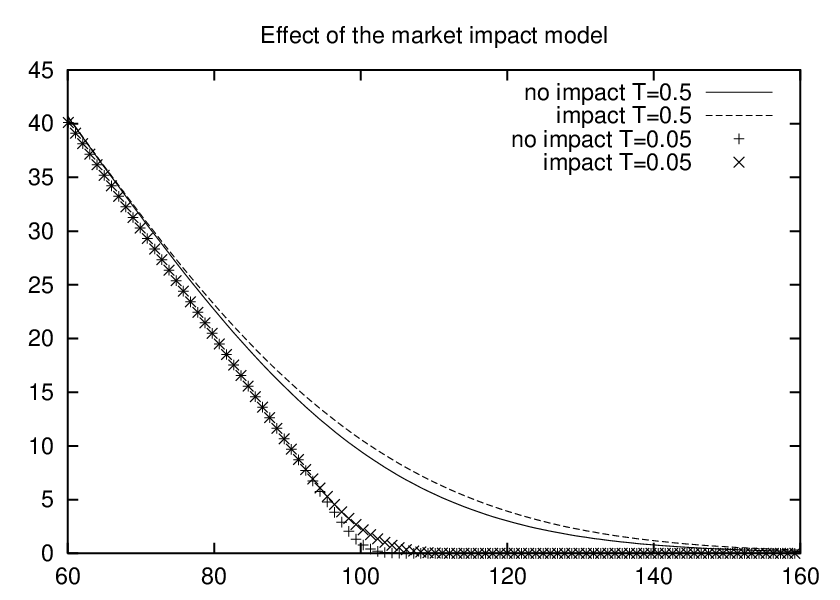
Refer to caption
(a) The case a put option (gamma short case)
Refer to caption
(b) The case of a put option(gamma long case)
Refer to caption
(c) The call spread case
Table 1. Numerical Simulations

Appendix A

A.1. Proof of Theorem 5.17

We perform the change of variable s=eys=e^{y}, and consider vi(t,y)=ui(t,ey),i=1,2v_{i}(t,y)=u_{i}(t,e^{y}),i=1,2, which yields that s2​∂s​sui=∂y​yvi−∂yvis^{2}\partial_{ss}u_{i}=\partial_{yy}v_{i}-\partial_{y}v_{i}. Under the above assumptions, u1u_{1} and u2u_{2} have logarithmic growth near 00 and linear growth at +∞+\infty, hence v1,v2v_{1},v_{2} have exponential growth. The derivatives of viv_{i} with respect to yy are bounded up to order 3, and σ\sigma is uniformly Lipschitz as a function of yy. Then w=v1−v2w=v_{1}-v_{2} solves

∂tw+σ2​(t,ey)2​∂y​yw−∂yw(1−λ⁡(∂y​yv1−∂yv1))​(1−λ⁡(∂y​yv2−∂yv2))=0.\displaystyle\partial_{t}w+\frac{\sigma^{2}(t,e^{y})}{2}\frac{\partial_{yy}w-\partial_{y}w}{(1-\lambda(\partial_{yy}v_{1}-\partial_{y}v_{1}))(1-\lambda(\partial_{yy}v_{2}-\partial_{y}v_{2}))}=0.

This can be seen as a linear equation of the form

∂tw+a⁡(t,y)​∂y​yw+b⁡(t,y)​∂yw=0,\displaystyle\partial_{t}w+a(t,y)\partial_{yy}w+b(t,y)\partial_{y}w=0,

where a,ba,b are bouded, uniformly Lipschitz in yy, aa bounded away from 0. Then we can apply classical results of comparison under exponential growth (see [3]).

□\hfill\Box

Appendix B

B.1. Proof of Lemma 5.8

We consider 𝒴{\mathcal{Y}} introduced in (89) under the probability ℙ~\tilde{\mathbb{P}}, with Wℙ~W^{\tilde{\mathbb{P}}} a ℙ~\tilde{\mathbb{P}}-Brownian motion, and 𝔼ℙ~\mathbb{E}^{\tilde{\mathbb{P}}} the expectation under ℙ~\tilde{\mathbb{P}}. We drop the superscripts ℙ~\tilde{\mathbb{P}} for the rest of the proof proof. We need first the following Lemma:

Lemma B.1.

There exists κ0>0,C\kappa_{0}>0,C such that

(109) ∀κ≤κ0,∫ℝexp⁡(−x22​C​κ)​sups∈[κ,T]|w⁡(t,x)|​𝑑x<+∞.\displaystyle\forall\kappa\leq\kappa_{0},\int_{\mathbb{R}}\exp\left({-\frac{x^{2}}{2C\kappa}}\right)\sup_{s\in[\kappa,T]}|w(t,x)|dx<+\infty.

Proof of Lemma B.1. First note that ww is concave, increasing and ∂xw\partial_{x}w has limit equal to 0 at +∞+\infty. Then since σ≤σ¯\sigma\leq\bar{\sigma},

(110) dd​t(w(t,x+12σ¯2(t−T)))=−12σ2∂x​xw+12(σ¯2−σ2)∂xw≥0,\displaystyle\frac{d}{dt}\left(w(t,x+\frac{1}{2}\bar{\sigma}^{2}(t-T))\right)=-\frac{1}{2}\sigma^{2}\partial_{xx}w+\frac{1}{2}(\bar{\sigma}^{2}-\sigma^{2})\partial_{x}w\geq 0,

hence t→w⁡(t,x+12​σ¯2​(t−T))t\to w(t,x+\frac{1}{2}\bar{\sigma}^{2}(t-T)) is non decreasing. The concavity of ww implies then that w⁡(t,x+12​σ¯2​(t−T))−wT​(0)−x​∂xwT​(0)w(t,x+\frac{1}{2}\bar{\sigma}^{2}(t-T))-w_{T}(0)-x\partial_{x}w_{T}(0) is non-positive. Then we consider 𝒴t{\mathcal{Y}}_{t} defined in (89). Note that as we assume that uu is a classical solution, then w∈Cs,t,l​o​c2,1w\in C^{2,1}_{s,t,loc}, and as moreover σ\sigma is bounded, 𝒴{\mathcal{Y}} is well defined. There holds that

(111) Xt=w⁡(t,𝒴t)−wT​(0)−∂xwT​(0)​(𝒴t+12​σ¯2​(T−t))\displaystyle X_{t}=w(t,{\mathcal{Y}}_{t})-w_{T}(0)-\partial_{x}w_{T}(0)({\mathcal{Y}}_{t}+\frac{1}{2}\bar{\sigma}^{2}(T-t))

is also non-positive and satisfies

d​Xt=(∂xw⁡(t,𝒴t)−∂xwT​(0))​σt​d​Wt+∂xwT​(0)​12​(σ¯2−σt2)​d​t.\displaystyle dX_{t}=(\partial_{x}w(t,{\mathcal{Y}}_{t})-\partial_{x}w_{T}(0))\sigma_{t}dW_{t}+\partial_{x}w_{T}(0)\frac{1}{2}(\bar{\sigma}^{2}-\sigma_{t}^{2})dt.

It is therefore a non-positive sub-martingale, and there holds by Fatou’s lemma

Xt\displaystyle X_{t} ≤\displaystyle\leq 𝔼⁡(Xt+s|ℱt)\displaystyle\mathbb{E}(X_{t+s}|{\mathcal{F}}_{t})
=\displaystyle= 𝔼⁡(w⁡(t+s,𝒴t+s|ℱt)−wT​(0)−∂xwT​(0)​(𝔼⁡(𝒴t+s|ℱt)+12​σ¯2​(T−t−s))CLOSE.\displaystyle\mathbb{E}(w(t+s,{\mathcal{Y}}_{t+s}|{\mathcal{F}}_{t})-w_{T}(0)-\partial_{x}w_{T}(0)\left(\mathbb{E}({\mathcal{Y}}_{t+s}|{\mathcal{F}}_{t})+\frac{1}{2}\bar{\sigma}^{2}(T-t-s)\right).

This implies that 𝔼⁡(w⁡(t+s,𝒴t+s|ℱt)CLOSE\mathbb{E}(w(t+s,{\mathcal{Y}}_{t+s}|{\mathcal{F}}_{t}) is finite. Then using the concavity and monotonicity of ww and Itô’s formula, one has

(112) 𝔼⁡(w⁡(t+s,𝒴t+s|ℱt)≤𝔼⁡(w⁡(t+s,𝒴t+σ¯​Ws+12​σ¯2​s)CLOSECLOSE\displaystyle\mathbb{E}(w(t+s,{\mathcal{Y}}_{t+s}|{\mathcal{F}}_{t})\leq\mathbb{E}(w(t+s,{\mathcal{Y}}_{t}+\underline{\sigma}W_{s}+\frac{1}{2}\bar{\sigma}^{2}s)

which shows that for t+s≤Tt+s\leq T,

1(2​π​s)12​∫ℝexp⁡(−x22​σ¯2​s)​|w⁡(t+s,x)|​𝑑x\displaystyle\frac{1}{(2\pi s)^{\frac{1}{2}}}\int_{\mathbb{R}}\exp\left({-\frac{x^{2}}{2\underline{\sigma}^{2}s}}\right)|w(t+s,x)|dx

is finite as long as w⁡(t,⋅)w(t,\cdot) is finite. The conclusion of the proof then follows by observing that, from (110),

sups∈[t,T]|w⁡(s,x)|≤sups∈[t,T]|w⁡(t,x−12​σ2​(s−t))|.\displaystyle\sup_{s\in[t,T]}|w(s,x)|\leq\sup_{s\in[t,T]}|w(t,x-\frac{1}{2}\sigma^{2}(s-t))|.

□\hfill\Box

We now go back to the proof of Lemma 5.8. Since ∂xw=1𝒮\partial_{x}w=\frac{1}{{\mathcal{S}}}, by standard manipulations on the heat kernel, (51) implies that for some ε>0\varepsilon>0,

(113) ∫ℝexp⁡(−x22​σ¯2​(T+ε))​wT​(x)​𝑑x\displaystyle\int_{\mathbb{R}}\exp\left(-\frac{x^{2}}{2\bar{\sigma}^{2}(T+\varepsilon)}\right)w_{T}(x)dx

is finite, hence w¯\bar{w} is defined on (−ε,T)(-\varepsilon,T) and limt→Tw⁡(t,x)=wT\lim_{t\to T}w(t,x)=w_{T}. Observe that w¯\bar{w} (resp. OPENw¯)\underline{w}) is solution to

∂tw¯+12​(σ¯2​∂x​xw¯+σ¯2​∂xw¯)\displaystyle\partial_{t}\bar{w}+\frac{1}{2}(\bar{\sigma}^{2}\partial_{xx}\bar{w}+\underline{\sigma}^{2}\partial_{x}\bar{w}) =\displaystyle= 0,\displaystyle 0,
w¯​(T,⋅)\displaystyle\bar{w}(T,\cdot) =\displaystyle= wT,\displaystyle w_{T},

(resp.

∂tw¯+12​(σ¯2​∂x​xw¯+σ¯2​∂xw¯)\displaystyle\partial_{t}\underline{w}+\frac{1}{2}(\underline{\sigma}^{2}\partial_{xx}\underline{w}+\bar{\sigma}^{2}\partial_{x}\underline{w}) =\displaystyle= 0,\displaystyle 0,
w¯​(T,⋅)\displaystyle\underline{w}(T,\cdot) =\displaystyle= OPENwT).\displaystyle w_{T}).

We write for ww

∂tw+12​σ¯2​∂x​xw+12​σ¯2​∂xw=12​(σ¯2−σ2)​∂x​xw−12​(σ2−σ¯2)​∂xw.\displaystyle\partial_{t}w+\frac{1}{2}\bar{\sigma}^{2}\partial_{xx}w+\frac{1}{2}\underline{\sigma}^{2}\partial_{x}w=\frac{1}{2}(\bar{\sigma}^{2}-\sigma^{2})\partial_{xx}w-\frac{1}{2}(\sigma^{2}-\underline{\sigma}^{2})\partial_{x}w.

We consider S=12​(σ¯2−σ2)​∂x​xw−12​(σ2−σ¯2)​∂xwS=\frac{1}{2}(\bar{\sigma}^{2}-\sigma^{2})\partial_{xx}w-\frac{1}{2}(\sigma^{2}-\underline{\sigma}^{2})\partial_{x}w, which is non-positive. From the concavity and monotonicity of ww, one obtains by simple calculations that if ww satisfies (109) for some ε1\varepsilon_{1}, then ∂xw\partial_{x}w and ∂x​xw\partial_{xx}w and hence SS also satisfy (109) for any ε2<ε1\varepsilon_{2}<\varepsilon_{1}. Consider then w~\tilde{w} defined by

w~(t,x)=−∫tT1σ¯​2​π​(t′−t)∫ℝexp(−(x+12​σ¯2​(t′−t)−z)22​σ¯2​(t′−t))S(t′,z)dzdt′.\displaystyle\tilde{w}(t,x)=-\int_{t}^{T}\frac{1}{\bar{\sigma}\sqrt{2\pi(t^{\prime}-t)}}\int_{\mathbb{R}}\exp\left(-\frac{(x+\frac{1}{2}\underline{\sigma}^{2}(t^{\prime}-t)-z)^{2}}{2\bar{\sigma}^{2}(t^{\prime}-t)}\right)S(t^{\prime},z)dzdt^{\prime}.

Then since S⁡(t′,z)S(t^{\prime},z) satisfies (109), w~\tilde{w} is well defined for t∈[T−τ,T]t\in[T-\tau,T] for some τ>0\tau>0, and solves

∂tw~+12​σ¯2​∂x​xw~−12​σ¯2​∂xw~=S\displaystyle\partial_{t}\tilde{w}+\frac{1}{2}\bar{\sigma}^{2}\partial_{xx}\tilde{w}-\frac{1}{2}\underline{\sigma}^{2}\partial_{x}\tilde{w}=S

with w~​(T)=0\tilde{w}(T)=0. Finally we have

w=w~+w^,\displaystyle w=\tilde{w}+\hat{w},

where w^\hat{w} satisfies

(114) ∂tw^+12​σ¯2​∂x​xw^−12​σ¯2​∂xw^=0,\displaystyle\partial_{t}\hat{w}+\frac{1}{2}\bar{\sigma}^{2}\partial_{xx}\hat{w}-\frac{1}{2}\underline{\sigma}^{2}\partial_{x}\hat{w}=0,

with w^​(T)=wT\hat{w}(T)=w_{T}, and w^\hat{w} satisfies (109). Then we have the following lemma:

Lemma B.2.

There exists τ⁡(κ)\tau(\kappa) such that, on [T−τ,T][T-\tau,T], there exists a unique solution of (114) that satisfies (109) with parameter κ\kappa.

Proof. This is a straightforward adaptation of the proof of Tychonoff [35]. The inequality obtained there page 207 adapted to our case is

|w|​(t,x)≤f⁡(−R)​exp−(x+R)22​σ¯2​t​tT+f⁡(R)​exp−(x−R)22​σ¯2​t​tT,\displaystyle|w|(t,x)\leq f(-R)\exp{-\frac{(x+R)^{2}}{2\bar{\sigma}^{2}t}}\sqrt{\frac{t}{T}}+f(R)\exp{-\frac{(x-R)^{2}}{2\bar{\sigma}^{2}t}}\sqrt{\frac{t}{T}},

with f⁡(A)=sup0≤t≤T{|w⁡(t,A)|}f(A)=\sup_{0\leq t\leq T}\{|w(t,A)|\}. Choosing tt small enough so that the right hand side is integrable leads to the conclusion that w⁡(t,x)=0w(t,x)=0.

□\hfill\Box

Since ww and w~\tilde{w} satisfy the growth condition (109), Lemma B.2 implies that w^\hat{w} is indeed equal to w¯\bar{w} defined above up to TτT_{\tau}. The argument can then be repeated up to T−n​τT-n\tau and yields uniqueness up to t=0t=0. Then w=w~+w¯w=\tilde{w}+\bar{w}, where w~\tilde{w} is non negative, hence we conclude w≥w¯w\geq\bar{w}. The other inequality w≤w¯w\leq\underline{w} follows directly from (112).

□\hfill\Box

B.2. Proof of Lemma 6.9

To prove the equi-integrability of w⁡(t,𝒴t)∧0w(t,{\mathcal{Y}}_{t})\wedge 0, we will use Lemma 5.8, hence for all K>0K>0

𝔼ℙ~​(w⁡(t,𝒴t)+K)−\displaystyle\mathbb{E}^{\tilde{\mathbb{P}}}\left(w(t,{\mathcal{Y}_{t}})+K\right)^{-} ≥\displaystyle\geq 𝔼ℙ~​(w¯​(t,𝒴t)+K)−\displaystyle\mathbb{E}^{\tilde{\mathbb{P}}}\left(\bar{w}(t,{\mathcal{Y}_{t}})+K\right)^{-}
≥\displaystyle\geq 𝔼ℙ~​(w¯​(t,𝒴0+σ¯​Wt+σ¯22​t)+K)−,\displaystyle\mathbb{E}^{\tilde{\mathbb{P}}}\left(\bar{w}(t,{\mathcal{Y}}_{0}+\bar{\sigma}W_{t}+\frac{\underline{\sigma}^{2}}{2}t)+K\right)^{-},

where the last line comes by using the concavity and the the monotonicity of w¯\bar{w}. As has been observed already, ∂xw⁡(t,𝒮)=1𝒮\partial_{x}w(t,{\mathcal{S}})=\frac{1}{{\mathcal{S}}}, hence by standard computations on the heat kernel, the last line is uniformly bounded under (51). Hence for t∈[0,T]t\in[0,T],

0≥𝔼ℙ~​(w⁡(t,𝒴t)+K)−≥−δ⁡(K),\displaystyle 0\geq\mathbb{E}^{\tilde{\mathbb{P}}}\left(w(t,{\mathcal{Y}_{t}})+K\right)^{-}\geq-\delta(K),

where limK→+∞δ⁡(K)=0\lim_{K\to+\infty}\delta(K)=0. By Chebyshev’s inequality, this implies that

𝔼ℙ~​(K​𝕀w≤−2​K)≤δ⁡(K),\displaystyle\mathbb{E}^{\tilde{\mathbb{P}}}\left(K\mathbb{I}_{w\leq-2K}\right)\leq\delta(K),

hence that

𝔼ℙ~​(K​𝕀w≤−K)≤2​δ​(K/2),\displaystyle\mathbb{E}^{\tilde{\mathbb{P}}}\left(K\mathbb{I}_{w\leq-K}\right)\leq 2\delta(K/2),

Finally summing the two we have that

𝔼ℙ~​(w⁡(t,𝒴t)​𝕀w≤−K)≥−(δ⁡(K)+2​δ​(K/2)).\displaystyle\mathbb{E}^{\tilde{\mathbb{P}}}\left(w(t,{\mathcal{Y}_{t}})\mathbb{I}_{w\leq-K}\right)\geq-(\delta(K)+2\delta(K/2)).

□\hfill\Box

Appendix C

C.1. Proof of Theorem 5.13

Under the condition λ​s2​∂s​sΦ≤1\lambda s^{2}\partial_{ss}\Phi\leq 1, lims→∞∂sΦ=ℒ∈ℝ∪{−∞}\lim_{s\to\infty}\partial_{s}\Phi={\mathcal{L}}\in\mathbb{R}\cup\{-\infty\}. We first prove the following Lemma:

Lemma C.1.

Let Φ\Phi satisfy assumption (51). For all τ>0\tau>0, for all κ′>0\kappa^{\prime}>0 small, there exists (K,κ)​(τ,κ′)(K,\kappa)(\tau,\kappa^{\prime}) , such that for t′∈[0,T−τ]t^{\prime}\in[0,T-\tau],

[κ′,1/κ′]⊂∂yv∗​(t′,[−K,Kℒ])⊂[κ,1/κ],\displaystyle[\kappa^{\prime},1/\kappa^{\prime}]\subset\partial_{y}v^{*}(t^{\prime},[-K,K_{\mathcal{L}}])\subset[\kappa,1/\kappa],

where

Kℒ={ℒ−1K​ if ​ℒ​ is finiteK​ otherwise.\displaystyle K_{\mathcal{L}}=\left\{\begin{array}[]{ll}{\mathcal{L}}-\frac{1}{K}\text{ if }{\mathcal{L}}\text{ is finite}\\ K\text{ otherwise.}\end{array}\right.

The constants K,κK,\kappa depend only on the behaviour at −∞-\infty and +∞+\infty of wTw_{T}

Proof of Lemma C.1 We start by constructing two barriers as in the proof of Theorem 5.7: v¯,v¯\bar{v},\underline{v} are the inverse of w¯,w¯\bar{w},\underline{w} defined by (60, 61) in Lemma 5.8, and w¯≤w≤w¯\bar{w}\leq w\leq\underline{w}, which then yields v¯≤v∗≤v¯.\underline{v}\leq v^{*}\leq\bar{v}. From the construction of wTw_{T} (see Proposition 5.3, point 8), under assumption (51) there holds

lims→0ln⁡(s)+λ⁡(Φ−s​∂sΦ)\displaystyle\lim_{s\to 0}\ln(s)+\lambda(\Phi-s\partial_{s}\Phi) =\displaystyle= −∞,\displaystyle-\infty,
lims→0−1s−λ∂sΦ\displaystyle\lim_{s\to 0}-\frac{1}{s}-\lambda\partial_{s}\Phi =\displaystyle= −∞.\displaystyle-\infty.

and moreover

wT​(ln⁡(s)+λ⁡(Φ−s​∂sΦ))\displaystyle w_{T}(\ln(s)+\lambda(\Phi-s\partial_{s}\Phi)) =\displaystyle= −1s−λ​∂sΦ,\displaystyle-\frac{1}{s}-\lambda\partial_{s}\Phi,
∂xwT​(ln⁡(s)+λ⁡(Φ−s​∂sΦ))\displaystyle\partial_{x}w_{T}(\ln(s)+\lambda(\Phi-s\partial_{s}\Phi)) =\displaystyle= 1s,\displaystyle\frac{1}{s},

which imply that

(116) limx→−∞∂xwT\displaystyle\lim_{x\to-\infty}\partial_{x}w_{T} =\displaystyle= +∞,\displaystyle+\infty,
(117) limx→+∞∂xwT\displaystyle\lim_{x\to+\infty}\partial_{x}w_{T} =\displaystyle= 0,\displaystyle 0,
(118) limx→+∞wT\displaystyle\lim_{x\to+\infty}w_{T} =\displaystyle= −λ​ℒ∈ℝ∪+∞.\displaystyle-\lambda{\mathcal{L}}\in\mathbb{R}\cup+\infty.

Limits (116, 117, 118) are propagated for time t≤Tt\leq T and, for t<Tt<T, w¯\bar{w} and w¯\underline{w} are strictly increasing. Moreover, as noted in (110), t→w⁡(t,x+σ¯22​(t−T))t\to w(t,x+\frac{\bar{\sigma}^{2}}{2}(t-T)) is non decreasing, hence

w¯​(0,x−σ¯22​t)≤w⁡(t,x)≤w¯​(T−τ,x+σ¯22​(T−τ−t)).\displaystyle\bar{w}(0,x-\frac{\bar{\sigma}^{2}}{2}t)\leq w(t,x)\leq\underline{w}(T-\tau,x+\frac{\bar{\sigma}^{2}}{2}(T-\tau-t)).

The concavity of ww and (116, 117, 118) imply then a control on the way in which ww goes to −∞-\infty at −∞-\infty and goes to +∞+\infty as +∞+\infty, which passing to v∗v^{*} yields the lemma.

□\hfill\Box

Proof of Theorem 5.13. We study (57) on compact sets of (∞,−λ​ℒ)×[0,T−τ](\infty,-\lambda{\mathcal{L}})\times[0,T-\tau] for small τ\tau. From Lemma C.1, we see that (57) is uniformly parabolic and that we have an a priori bound for v∗v^{*} and ∂yv∗\partial_{y}v^{*}. We can thus apply Lemma 5.11, to obtain local Cx1+αC^{1+\alpha}_{x} regularity for v∗v^{*} for time t<Tt<T. As in the proof ot Theorem 5.7, equation (57) on v∗v^{*} can now be seen as a linear parabolic equation with Hölder coefficients, and Schauder estimates then yield that v∗∈Ct,x,l​o​c1+α/2,2+α​([0,T)×(−∞,−λ​ℒ))v^{*}\in C^{1+\alpha/2,2+\alpha}_{t,x,loc}([0,T)\times(-\infty,-\lambda{\mathcal{L}})). By differentiating the equation, further regularity follows if σ\sigma has additional regularity. Then using the left side of the inequality in Lemma C.1, the local regularity of v∗v^{*} on (−∞,−λ​ℒ)(-\infty,-\lambda{\mathcal{L}}) implies local regularity of vv on ℝ+∗\mathbb{R}_{+}^{*}, henceforth of uu on any compact set of [0,T)×ℝ+∗[0,T)\times\mathbb{R}_{+}^{*}. This achieves the proof of Theorem 5.13.

□\hfill\Box

Appendix D Existence of smooth solutions for general λ\lambda

Here we state a simple result of smoothness for ”good” initial data in the case where λ=λ⁡(γ)\lambda=\lambda(\gamma), when σ\sigma is constant. In this case, we need to start with well behaved solutions, as the singularity of the solution can not be treated by the Legendre transform technique of the previous section. What we show is the following:

Theorem D.1.

Let the final payoff Φ\Phi satisfy

(119) −1ε≤λ​s2​∂s​sΦ≤1−ε\displaystyle-\frac{1}{\varepsilon}\leq\lambda s^{2}\partial_{ss}\Phi\leq 1-\varepsilon

for some ε>0\varepsilon>0. Assume that λ⁡(γ)\lambda(\gamma) is smooth satisfies locally uniformly with respect to γ\gamma the condition (28). Then there exists a smooth solution to (22, 23, 24) such that (119) is satisfied for all time, that belongs to Cs,t2+α,1+α/2​([0,T)×ℝ+∗)C^{2+\alpha,1+\alpha/2}_{s,t}([0,T)\times\mathbb{R}_{+}^{*}).

Proof. We only sketch the proof, this is an adaptation of Propositon 5.15 that relies on the estimate formula 73. This is a simple consequence of the identity (73). From this and the conditions on the boundary data Φ\Phi, one can construct a solution such that (73) holds and γ\gamma remains bounded above and below. Then classical parabolic regularity theory yields the result.

□\hfill\Box

We make the following observation:

Proposition D.2.

Let 0∈I0\in I, F:γ∈I→ℝF:\gamma\in I\to\mathbb{R} be a smooth increasing function such that F⁡(0)=0F(0)=0 and F⁡(γ)≥γF(\gamma)\geq\gamma. Then there exists λ⁡(γ)≥0\lambda(\gamma)\geq 0 such that

F⁡(γ)=γ1−λ⁡(γ)​γ.\displaystyle F(\gamma)=\frac{\gamma}{1-\lambda(\gamma)\gamma}.

Moreover λ=1γ−1F\lambda=\frac{1}{\gamma}-\frac{1}{F}.

This comes by elementary computations, and shows that under mild conditions on FF, any fully non-linear pde of the form ∂tu+12​σ2​F​(s2​∂s​su)=0\partial_{t}u+\frac{1}{2}\sigma^{2}F(s^{2}\partial_{ss}u)=0 can be derived as a market impact pricing equation. Note that the conditions imply F′​(0)=1F^{\prime}(0)=1 and F′′​(0)≥0F^{\prime\prime}(0)\geq 0.

References

  • [1] Frédéric Abergel and Grégoire Loeper. Pricing and hedging contingent claims with liquidity costs and market impact. To appear in the proceedings of the International Workshop on Econophysics and Sociophysics, Springer, New Economic Window, 2016.
  • [2] R.A. Almgren. Equity market impact. RISK, July, 2005.
  • [3] Andrea Pascucci (auth.). PDE and Martingale Methods in Option Pricing. Bocconi & Springer Series. Springer-Verlag Mailand, 1 edition, 2011.
  • [4] G. Barles. Solutions de viscosité des équations de Hamilton-Jacobi. Mathématiques & Applications [Mathematics & Applications], 17. Springer-Verlag, Paris, 1994.
  • [5] B. Bouchard, G. Loeper, and Y. Zou. Almost sure hedging with permanent price impact. Finance stoch. to appear.
  • [6] B. Bouchard, G. Loeper, and Y. Zou. Hedging of covered options in a linear market impact model. http://arxiv.org/abs/1512.07087.
  • [7] Y. Brenier. Polar factorization and monotone rearrangement of vector-valued functions. Comm. Pure Appl. Math., 44(4):375–417, 1991.
  • [8] Umut Çetin, Robert A. Jarrow, and Philip Protter. Liquidity risk and arbitrage pricing theory. Finance Stoch., 8(3):311–341, 2004.
  • [9] Umut Çetin, H. Mete Soner, and Nizar Touzi. Option hedging for small investors under liquidity costs. Finance Stoch., 14(3):317–341, 2010.
  • [10] Patrick Cheridito, H. Mete Soner, Nizar Touzi, and Nicolas Victoir. Second-order backward stochastic differential equations and fully nonlinear parabolic PDEs. Comm. Pure Appl. Math., 60(7):1081–1110, 2007.
  • [11] Michael Crandall and Michel Pierre. Regularizing effects for ut+A​φ​(u)=0u_{t}+A\varphi(u)=0 in L1L^{1}. J. Funct. Anal., 45(2):194–212, 1982.
  • [12] Michael G. Crandall, Hitoshi Ishii, and Pierre-Louis Lions. User’s guide to viscosity solutions of second order partial differential equations. Bull. Amer. Math. Soc. (N.S.), 27(1):1–67, 1992.
  • [13] Michael G. Crandall and Michel Pierre. Regularizing effects for ut=Δ​φ​(u)u_{t}=\Delta\varphi(u). Trans. Amer. Math. Soc., 274(1):159–168, 1982.
  • [14] R. Frey. Perfect option hedging for a large trader. Finance and Stochastics, 2(2):115–141.
  • [15] R. Frey and A. Stremme. Market volatility and feedback effects from dynamic hedging. Mathematical Finance, 7(4):351–374, 1997.
  • [16] D. Gilbarg and N. S. Trudinger. Elliptic partial differential equations of second order, volume 224 of Grundlehren der Mathematischen Wissenschaften [Fundamental Principles of Mathematical Sciences]. Springer-Verlag, Berlin, second edition, 1983.
  • [17] L. V. Kantorovich. On mass transportation. Dokl. Akad. Nauk. SSSR, 37:227–229, 1942.
  • [18] L. V. Kantorovich. On a problem of Monge. Uspekhi Mat.Nauk., 3:225–226, 1948.
  • [19] Ioannis Karatzas and Steven E. Shreve. Brownian motion and stochastic calculus, volume 113 of Graduate Texts in Mathematics. Springer-Verlag, New York, second edition, 1991.
  • [20] Robert V. Kohn and Sylvia Serfaty. A deterministic-control-based approach to fully nonlinear parabolic and elliptic equations. Comm. Pure Appl. Math., 63(10):1298–1350, 2010.
  • [21] D. Lamberton, H. Pham, and M. Schweizer. Local risk-minimization under transaction costs. Mathematics of Operations Research, 23:585–612, 1997.
  • [22] Gary M. Lieberman. Second order parabolic differential equations. World Scientific, Singapore, River Edge (N.J.), 1996. Réimpression : 1998.
  • [23] H. Liu and J. M. Yong. Option pricing with an illiquid underlying asset market. Journal of Economic Dynamics and Control, 29:2125–2156, 2005.
  • [24] G. Loeper. The reconstruction problem for the Euler-Poisson system in cosmology. Arch. Ration. Mech. Anal., 179(2):153–216, 2006.
  • [25] H. M. Soner P. Cheridito and N. Touzi. The multi-dimensional super-replication problem under gamma constraints. Annales de l’’Institut Henri Poincaré, Série C: Analyse Non-Linéaire, 22:633–666, 2005.
  • [26] E. Platen and M. Schweizer. On feedback effects from hedging derivatives. Mathematical Finance, 8(1):67–84, 1998.
  • [27] R. T. Rockafellar. Convex analysis. Princeton Landmarks in Mathematics. Princeton University Press, Princeton, NJ, 1997. Reprint of the 1970 original, Princeton Paperbacks.
  • [28] P. J. Schönbucher and P. Wilmott. The feedback effect of hedging in illiquid markets. SIAM J. Appl. Maths, 61(1):232–272, 2000.
  • [29] H. M. Soner and N. Touzi. Superreplication under gamma constraints. SIAM J. Control Optim., 39:73–96, 2000.
  • [30] H. M. Soner and N. Touzi. Dynamic programming for stochastic target problems and geometric flows. Journal of the European Mathematical Society, 4:201–236, 2002.
  • [31] H. M. Soner and N. Touzi. Hedging under gamma constraints by optimal stopping and face-lifting. Mathematical finance, 17:59–80, 2007.
  • [32] H. Mete Soner, Nizar Touzi, and Jianfeng Zhang. Dual formulation of second order target problems. Ann. Appl. Probab., 23(1):308–347, 2013.
  • [33] Xiaolu Tan and Nizar Touzi. Optimal transportation under controlled stochastic dynamics. Ann. Probab., 41(5):3201–3240, 2013.
  • [34] B. Tóth, Z. Eisler, F. Lillo, J. Kockelkoren, J.-P. Bouchaud, and J. D. Farmer. How does the market react to your order flow? Quant. Finance, 12(7):1015–1024, 2012.
  • [35] A. Tychonoff. Théorèmes d’unicité pour l’équation de la chaleur. Rec. Math. Moscou, 42(2):199–216, 1935.
  • [36] Juan Luis Vázquez. Smoothing and decay estimates for nonlinear diffusion equations, volume 33 of Oxford Lecture Series in Mathematics and its Applications. Oxford University Press, Oxford, 2006. Equations of porous medium type.
  • [37] C. Villani. Topics in optimal transportation, volume 58 of Graduate Studies in Mathematics. American Mathematical Society, Providence, RI, 2003.
  • [38] Xu-Jia Wang. Schauder estimates for elliptic and parabolic equations. Chinese Ann. Math. Ser. B, 27(6):637–642, 2006.

Gregoire Loeper
Monash University
School of Mathematics
9 Rainforest Walk
3800 CLAYTON VIC, AUSTRALIA

email: gregoire.loeper@monash.edu