Phases of large vector Chern-Simons theories on
Abstract:
We study the thermal partition function of level Chern-Simons theories on interacting with matter in the fundamental representation. We work in the ’t Hooft limit, , with and held fixed where is the temperature and the volume of the sphere. An effective action proposed in arXiv:1211.4843 relates the partition function to the expectation value of a ‘potential’ function of the holonomy in pure Chern-Simons theory; in several examples we compute the holonomy potential as a function of . We use level rank duality of pure Chern-Simons theory to demonstrate the equality of thermal partition functions of previously conjectured dual pairs of theories as a function of the temperature. We reduce the partition function to a matrix integral over holonomies. The summation over flux sectors quantizes the eigenvalues of this matrix in units of and the eigenvalue density of the holonomy matrix is bounded from above by . The corresponding matrix integrals generically undergo two phase transitions as a function of temperature. For several Chern-Simons matter theories we are able to exactly solve the relevant matrix models in the low temperature phase, and determine the phase transition temperature as a function of . At low temperatures our partition function smoothly matches onto the and independent free energy of a gas of non renormalized multi trace operators. We also find an exact solution to a simple toy matrix model; the large Gross-Witten-Wadia matrix integral subject to an upper bound on eigenvalue density.
1 Introduction
The AdS/CFT correspondence maps deconfinement transitions of large gauge theories on spheres to gravitational phase transitions involving black hole nucleation [1]. This observation has motivated the intensive study of deconfinement phase transitions of large dimensional Yang Mills theories (coupled to adjoint and fundamental matter) on . The thermal partition function of a Yang-Mills theory on is given by the Euclidean path integral of the theory on . Upon integrating out all massive modes this path integral reduces to an integral over the single unitary matrix
| (1) |
where is the zero mode (on ) of the holonomy around the thermal circle, () are the eigenvalues of . is a potential function whose precise form depends on the theory under study. At least in perturbation theory [2] and perhaps beyond [3, 4], the potential is an analytic function of . (1) may be thought of as a Landau Ginzburg or Wilsonian description of the holonomy , the lightest degree of freedom of the finite temperature field theory.
The effective potential was computed in free gauge theories [5, 2]; it has also been evaluated at higher orders in perturbation theory in special examples [6, 7, 8, 9]. In all these examples is an attractive potential for the eigenvalues of the unitary matrix. t’ Hooft counting and the requirement of extensivity force to scale like . In the special case of a conformal theory the potential scales like and the attraction between eigenvalues grows arbitrarily large at high temperatures.11 1 Most of the general discussion of this paragraph applies also to non conformal theories in the appropriate high temperature and/or large volume limit. On the other hand the integration measure (which vanishes when any two eigenvalues coincide) supplies a temperature independent repulsive potential for the eigenvalues. At large the leading piece of the partition function is determined by a saddle point distribution of eigenvalues of . Repulsion from the measure dominates over attraction from the potential at low temperatures and the eigenvalues of are distributed all over the unit circle in the complex plane.22 2 If the matter content of the theory consists only of fundamental plus adjoint fields, and if the matter content is held fixed as which is taken to infinity and the low temperature saddle point for is the clock matrix; a matrix whose eigenvalues are uniformly distributed on the unit circle in the complex plane. The integral (1) undergoes Gross-Witten-Wadia type deconfinement transitions [10, 11, 12] at of order unity.33 3 At weak coupling at least the system undergoes either a single first order transition or a second order transition followed by a third order phase transition depending on the details of a quartic term in the potential [2]. At high enough temperatures the saddle point eigenvalue distribution of has support on only a small arc in the unit circle of the complex plane. The size of this arc goes to zero as . In this ‘decompactification’ limit, the holonomy matrix is localized around the unit matrix.
In this note we study the finite temperature phase structure of renormalized level U() Chern-Simons theories coupled to a finite number of fundamental fields on in the t’ Hooft limit , with fixed.44 4 We use the dimensional reduction regulation scheme through this paper. In this case , where is the level of the Chern-Simons theory regulated by including an infinitesimal Yang Mills term in the action, and is the level of the theory regulated in the dimensional reduction scheme [13, 14]. For this reason this class of Chern-Simons theories may be well-defined only in the range . Hereafter we assume the ’t Hooft coupling is always positive for simplicity. Our results are easily generalized to the case is negative by taking the absolute value of it. We address the following question: Does the Landau Ginzburg description (1) continue to hold for Chern-Simons matter theories? If not what replaces it? Our analysis of this structural question applies to all fundamental matter Chern-Simons theories in the high temperature and large limit; in addition we make significant progress towards an exact determination of the partition function, the large free energy, as a function of temperature and , in particular examples of these theories.
To start our discussion let us first review the behaviour of matter Chern-Simons theories in the free limit . In particular examples such a thermal partition function was studied in [15, 16, 17]. The free partition function continues to be governed by the Landau Ginzburg form (1) even at finite ; in fact the only qualitative difference from the Yang Mills case is that scales like (rather than ) at high temperatures.55 5 The potential scales like rather than because the matter is in the fundamental representation and pure Chern-Simons theory has no propagating degrees of freedom. As the repulsion from the measure in (1) continues to scale like , the partition function displays interesting dynamics in the large limit only if we set and take the limit holding fixed. At small the eigenvalue density of the holonomy matrix has support everywhere on the unit circle in the complex plane; however at of order unity the system undergoes a third order clumping or deconfinement phase transition. At higher temperature the eigenvalue distribution has support only on a finite arc (centered about unity) on the complex plane. In the infinite limit the size of this arc goes to zero and the holonomy reduces to the identity matrix.
Large fundamental matter Chern-Simons theories have recently been studied intensively at finite values of the t’ Hooft coupling (see e.g. [16, 18, 19, 20, 21, 17, 22, 23, 24, 25, 26, 27]). In particular it has been argued in the important recent paper [27] that the entire effect of matter loops on gauge dynamics, at temperatures of order and at leading order in , is to generate a term of the form
for the gauge theory effective action. Here is an effective potential of order ,66 6 The trace of is counted as order . An example of a potential of order is whose detailed form depends on the matter content and couplings of the Chern-Simons matter system. It follows that in the large limit, the thermal Chern-Simons matter path integral is given by
| (2) |
(2) is simply the pure Chern-Simons theory with an added potential the local value of the holonomy matrix . As pure Chern-Simons theory is topological, the expectation values of observables are independent of and (2) may be rewritten as
| (3) |
where denotes the expectation value of in the pure Chern-Simons theory at rank and level and is the proper volume of the spatial manifold ( in this case). In other words the partition function of the matter Chern-Simons theory may be re-expressed as a linear combination of Wilson loops (in various representations of ) that wind the time circle. The only memory of the fundamental matter lies in the form of the function , whose structure is determined by the fundamental matter content and interactions.
Before turning to the important question of how may be determined in any given matter Chern-Simons theory, we pause to note an important property of the formula (3). As (3) is the expectation value of (a sum of) Wilson loops in rank and (renormalized) level Chern-Simons theory, the well established level rank duality of pure Chern-Simons theory relates the expectation value in (3) to the expectation value of a dual operator in rank and level pure Chern-Simons theory.77 7 If we use the unrenormalized Chern-Simons level then the level rank duality states the invariance of pure Chern-Simons theory under the exchange of and . (see [28, 29] for a relatively recent discussion of level rank duality and references to earlier work). The specific relationship turns out to be the following. Any gauge invariant function may be regarded as a function of the variables . For any such function we define a corresponding dual function by the equation
| (4) |
Level rank duality of pure Chern-Simons theory turns out to imply that
| (5) |
(5) will have interesting implications for matter Chern-Simons theories as we will see below.
Let us now return to computation of for any given Chern-Simons matter theory. It is a remarkable fact that the function appears to be exactly computable as a function of in the large limit for arbitrary matter Chern-Simons theories. As is an ultra local expression (i.e depends only on the value of at a point and not its derivatives; similarly is independent of the derivatives of the metric - i.e. curvatures - at the point ) it may be computed on rather than . Using standard large techniques and employing an unusual lightcone gauge, the authors of [16] were able to compute for the special case that as an arbitrary function of for the theory of fundamental fermions minimally coupled to the Chern-Simons field. This computation was later generalized to other theories in [23],[30]. It was also generalized to the computation of for a matrix whose eigenvalue distribution is given by (10) below (more below on why this is important) in [27]. A straightforward generalization of these computations permits the evaluation of for arbitrary ; our results for are presented in section 3 below for several examples of matter Chern-Simons theories. Pairs of the matter Chern Simons theories we have studied in section 3 below have been conjectured to be related via level rank type dualities. In section 3 below we demonstrate that, in each case, the potentials for conjecturally dual Chern-Simons matter theories are related by (4). It follows from (5) above that partition functions for conjectural dual matter Chern-Simons theory pairs are equal at every value of and temperature. Such dual pairs include Giveon-Kutasov duals for a chiral theory [31], minimally coupled fermions and gauged critical bosons, as well as minimally coupled bosons with gauged critical fermions [20, 22, 27, 26], see also [16] for a preliminary suggestion for duality. Our results may be viewed as additional evidence in support of these conjectured dualities.
In order to find explicit formulas for the partition function of Chern-Simons matter theories on we need to evaluate the expectation value (3). This may be achieved using path integral techniques. In fact the partition function of Chern-Simons theories on was evaluated by using path integral techniques long ago in the beautiful older paper [32], the analysis in [32] is easily generalized to include the effect of . Briefly (see section 4 for details) we follow [32] and work in the ‘temporal’ gauge (in this paper the Euclideanized time direction is so denotes temporal component of the gauge field). We then abelianize the residual two dimensional gauge invariance by an additional gauge fixing condition; the holonomy matrix is required to be diagonal. The integral over the off diagonal and Kaluza Klein modes of the spatial part of the gauge field is quadratic and yields a determinant, which turns out to largely cancel the Fadeev-Popov determinant of gauge fixing. The integral of the diagonal (unfixed abelian part) of the two dimensional gauge field yields a delta function that fixes to be constant on . And the summation of flux sectors discretizes the eigenvalues of in units of . These manipulations reduce the expectation value (3) to a ‘discretized’ version of integral over the holonomy matrix (1)
| (6) |
where
| (7) |
and is the unitary matrix whose eigenvalues are , where with running from to . Notice that the discretization interval between two allowed values of eigenvalues in (6), , tends to zero in the ’t Hooft limit . It follows that the eigenvalue density function in discretized one (6) and non-discretized one (1) obey identical large saddle point equations upon identifying the two potentials. Nonetheless the saddle points of (6) and (1) in the ’t Hooft limit are not always identical. Recall that the classical large saddle point descriptions of (6) and (1) are written in terms of the eigenvalue density function defined by
| (8) |
As the summation in (6) effectively excludes terms with coincident ’s,88 8 In the case that the base manifold is an , as studied in our paper, the exclusion of such configurations follows from the fact that the measure factor in (1) eliminates their contributions. The generalization of (6) to the partition function of Chern-Simons theory on where is a genus manifold of arbitrary metric is given by the formula (88). In these cases the measure factors is either constant (in the case of ) or diverges when two eigenvalues are equal. Nonetheless the correct prescription (the one that agrees with Chern-Simons computations using other techniques) appears to be to omit the contribution of such sectors. The justification for this prescription does not appear to be clearly understood from first principle path integral reasoning. We hope to clear up this point in the future. We thank O. Aharony, S. Giombi and J. Maldacena for extensive discussions on this point. it follows that the maximum number of eigenvalues in an interval in the summation in (6) is given by , so that the eigenvalue density (8) is bounded from above by . In other words the eigenvalue distribution in (6) is constrained to obey the inequalities
| (9) |
On the other hand for the integral (1) obeys the lower bound listed in (9) (this is because a density is an intrinsically positive quantity) but no upper bound.99 9 The same upper bound for the density function appears in two dimensional Yang-Mills theory (), in which case the situation becomes similar due to the fact that there is no propagating degrees of freedom for the gauge field. A phase transition relevant to this upper bound was studied in 2d (q-deformed) Yang-Mills theory on [33, 34, 35, 36], which we will see from Chern-Simons theory below. We noticed these relevant papers when we were completing this paper. Note that the upper bound in (9) agrees perfectly with the conclusions of [27], obtained using Hamiltonian methods for Chern-Simons theory on .
Any saddle point of (1) that happens to everywhere obey the inequality (9) is also a saddle point of (6). However saddle points of (1) that anywhere violate the upper bound (9) are not large solutions of (6). Instead (6) admits new classes of solutions; those that saturate the upper bound of the inequality (9) over one or more arcs along the unit circle. While saddle points of (1) may be classified in terms of the number of gaps in the solution (i.e. the number of arcs over which the eigenvalue density vanishes), saddle points of (6) are classified by the number of ‘lower gaps’ (regions over which the eigenvalue density vanishes) together with the number of ‘upper gaps’ (arcs over which the upper bound of (9) are saturated).
In order to understand the generic phase structure of matrix model (6) we found it useful to first study a toy model in which takes the simple Gross -Witten -Wadia form . We have found the exact solution to the saddle point equations of this toy model. The phase structure of this solution is depicted in Fig.6 (see §7.6 for a a more detailed summary of this solution); we pause to elaborate on this phase diagram. In this toy model it turns out that for the eigenvalue distribution has no gaps for , a single lower gap for and a lower gap plus an upper gap for . This sequence of eigenvalue distributions is depicted graphically in Fig. 7,7, 7, 7. For , on the other hand, the eigenvalue distribution has no gaps for , a single upper gap in the range , and an upper plus a lower gap for still larger . This phase sequence is depicted in Figure 8, 8, 8, 8 in §7.6. Moreover, in the large limit the eigenvalue distribution tends to the universal configuration
| (10) |
at every value of . The distribution (10) is the nearest thing to a function permitted by the effective Fermi statistics of the eigenvalues in perfect agreement with the results of the [27] which was the inspiration for the current work.
For any given matter Chern-Simons theory is more complicated than the toy model of the previous paragraph. Even for these more complicated functions , however, it turns out to be easy to solve exactly for the eigenvalue density function in the ‘no gap’ phase (see section 6 for details). The sequence of phases described above for the toy model is also true for every particular CS matter theory we have studied. Our exact solution allows us to determine the first phase transition temperature as a function of as well as the value of in the theories we have studied (the value of varies from theory to theory). On general grounds we expect the eigenvalue distribution to tend to the universal function (10) in the high temperature limit in all Chern-Simons matter theories, even though we have not (yet) found exact solutions to the relevant matrix models in the two gap phase.1010 10 Note that the case is special. In this case the number of distinct allowed ‘slots’ for the eigenvalues (number of distinct allowed values of ) is exactly equal to . As a consequence the eigenvalue distribution at is given by (11) at all values of the temperature. In this strong coupling limit the holonomy distributes uniformly around the circle.
We pause to describe an important property of our solution to the matrix model obtained from real Chern-Simons theories in the no gap phase at low temperature (for notational simplicity we work on a round sphere of volume in the rest of this paragraph). In the low temperature phase the partition function takes the form
In every theory we have studied, the Taylor expansion of the function takes form
| (12) |
where is a constant independent of . It follows that at very low temperatures
This is precisely the form of the partition function of a gas of multi ‘traces’; the value of the coefficient also works out to the value predicted by this expectation. The fact that the free energy is independent of at temperatures is in perfect agreement with the non renormalization theorem of the spectrum of single trace operators in these theories. In other words the results for the partition function obtained in this paper at small matches smoothly onto the high temperature expansion of the independent free energy.
We have explained above that the eigenvalue distributions of two theories related by level rank type dualities are related by the map
This relationship implies that the saddle point eigenvalue densities of two dual theories are related by the formula
where is the eigenvalue distribution of the theory with coupling while is the eigenvalue distribution of the theory with coupling . An interesting feature of this map is that it interchanges lower and upper gaps, consistent with the fact that the first phase transition is always from the no gap to the lower gap phase at small while it is from the no gap to the upper gap phase at near unity.
We end this introduction on a cautionary note. All of the results of this paper have been obtained starting from the effective action (2). While the arguments for this effective action presented in [27] and reviewed in subsection 2.1 below are persuasive, they are not completely beyond question. It would be useful to present a clear justification of (2) and understand how to compute corrections to the results from this action (such corrections are presumably suppressed in ). It would also be useful to better understand the exclusion of equal eigenvalues from (6). We feel that it is important to clear up these two issues before we can regard the large number of exact results presented in this paper as beyond reproach. We hope to return to these issues in the future.
2 Effective action and level rank duality
In this section we review the effective description of large Chern-Simons theories at temperature of order proposed in [27]. This effective description allows us to relate the partition function of any fundamental matter Chern-Simons theory, in an appropriate high temperature limit, to the expectation value of an appropriate ‘Wilson loop’ in the pure Chern-Simons theory. Using this fact we then explore the implications of level rank duality of Wilson loops in pure Chern-Simons theories for the partitions under study.
2.1 The high temperature effective action
Consider a Chern-Simons-fundamental matter theory on in the ’t Hooft large limit. As described in the introduction, we study a theory at very high temperatures with
| (13) |
where is held fixed in the large limit.
Our strategy for evaluating the partition function is, roughly speaking, first to find an effective action for the two dimensional holonomy field, , around the thermal (here is a point on the base ) by integrating out all other fields, and then to perform the path integral over two dimensional unitary matrix valued field . In practice we find it more convenient to break up the first step (computation of the effective action of ) into two steps as we now explain.
The effective action for is obtained by summing all vacuum graphs in which all non-holonomy fields appear in an unrestricted manner. We will find it useful to break up these graphs into those that involve at least one matter field, and those that do not. Let the result of summing over all graphs of the first sort be denoted by . Once we have , the remaining task is to sum over all graphs that do not involve a matter field; and then integrate over .1111 11 Our conventions of the gauge field are those of [37]. That is, the gauge field takes values of antihermitian matrix, the gauge covariant derivative is and its field strength is The gauge transformation is , where is a gauge parameter taking values of antihermitian matrix. The Chern-Simons action is (14) where Under an infinitesimal change of the action above changes as . In other words the full partition function is given in terms of by the formula
| (15) |
While the formula (15) is always correct in principle, it is useful in practice only when is a local function. The key observation of [27] is that is in fact ultralocal in the leading large limit, when the temperature is scaled as in (13). At leading order in large , in other words the effective action
| (16) |
(the power of temperature has been inserted on dimensional grounds, see below for more details) and the formula for the partition function are simplified to
| (17) |
The path integral in (17) is evaluated in Euclidean space and the temporal circle is compact with circumference .
The argument for the locality of is essentially that the graphs that we integrate out to find always include a matter propagator, and all matter fields develop large thermal masses. It appears to follow that can be expanded in a series of local operators in the form
| (18) |
where we have inserted powers of by dimensional analysis. Now the scaling (13) 1212 12 We are emphasizing that the partition function of fundamental matter -Chern-Simons theories are trivial (and independent) at temperatures of order unity. These partition functions have interesting (and generically dependent) structure only when the temperature is scaled as in (13). converts the high temperature expansion (18) into an expansion in inverse powers of . For instance the terms listed above are respectively of order , and . 1313 13 Every term in the effective action (18) is of order at fixed (powers of are counted as explained in the introduction), as the action is generated by integrating out fundamental fields. Terms that we have ignored in this expansion (the in (18)) are further suppressed at large . At leading order in the large expansion it seems to be justified to truncate (18) to the first term, yielding (17). 1414 14 [27] considered a slightly different effective action, one in which they integrated out all graphs of matter fields, Kaluza Klein modes of the gauge fields, but not the massless 2d gauge field. They expanded their effective action in the form (19) once again all terms but the first are sub leading in the expansion. It would be interesting to carefully investigate the relationship between and
The arguments leading up to (17) could conceivably have loopholes; in order to gain more confidence in (17) it would be useful to estimate the contributions of the neglected terms in (18) to the partition function and verify that their contribution is indeed sub leading in the expansion. We leave this exercise to future work.
In order to make (17) a concrete formula we must explain how the function may be computed for any particular vector matter Chern Simons theory. We take this question up in the next section, and present exact and reasonably explicit formulas - as a function of the ’t Hooft coupling for for sample matter Chern-Simons theories. In the rest of this section, however, we first explore a structural ‘duality’ of the formula (17).
2.2 Relations from level rank duality of pure Chern-Simons
The equation (17) may be rewritten as
| (20) |
where the symbol
denotes the expectation value of in pure Chern-Simons theory at level . As pure Chern-Simons theory is topological, an expectation value of the form
is independent of . It follows that (20) may be rewritten as
| (21) |
Recall that is a gauge invariant function of the holonomy matrix. Any such function may be expanded in a basis of characters of , i.e. in a basis of Polyakov or Wilson loops, in arbitrary representations of the gauge group , around the curve that winds the thermal circle. In other words the remarkable formula (21) relates the thermal partition function of fundamental matter Chern-Simons theories (in an appropriate coordinated high temperature and large limit) to the expectation value of a complicated thermal Wilson loop expectation value in pure Chern-Simons theory.
Now pure Chern-Simons theories of rank and renormalized level are dual to pure Chern-Simons theories of rank and level via the well known level rank duality. Wilson loops transform under this duality as follows: a Wilson loop in the representation labeled by the Young Tableaux maps to the Wilson loop in the representation labeled by Young Tableaux where and are related by ‘transposition’ (the interchange of rows with columns). This duality map for Wilson loops may be restated in a slightly simpler fashion for arbitrary gauge invariant functions (like ) of the holonomy matrix as we now explain.
The Wilson loop in any representation of is expressed as a polynomial of the variables () by the character polynomials of group theory. Let denote the character polynomial of the representation with Young Tableaux . Let denote the number of boxes in the Young Tableaux . The character polynomial of is given by the so called Schur Polynomial (see e.g. eq (2.15) of [38])
| (22) |
where the summation on the RHS runs over all elements of the permutation group , is the character of the permutation group element in the representation labeled by the Young Tableaux and , denote the number of cycles of length in the conjugacy class of the permutation element . We now recall that characters of the permutation group have a well known transformation property under transposition of the Young Tableaux
| (23) |
where is the sign of the permutation (see e.g. [39]). The sign of the permutation is given in terms of its number of cycles by
| (24) |
Plugging (23) and (24) into (22) we find
| (25) |
In other words transposition of Young Tableaux in all character polynomials (i.e. in arbitrary gauge invariant functions of ) is achieved by the uniform interchange1515 15 For the reader who dislikes appealing to mathematical authority for proofs, we present a ‘physics’ check of (25). Let denote the character polynomial of the representation with boxes in the first row of the Young Tableaux and no boxes in any other row. In a similar manner let denote the character polynomial of the representation with boxes in the first column of the Young Tableaux and no boxes in any other columns. Then it follows from the usual formulas of Bose and Fermi statistics that (26) where is any real number. Level rank duality interchanges and . At the level of the generating functions in (26) this interchange is simply achieved by (27).
| (27) |
It follows that level rank duality of pure Chern-Simons theory asserts that
| (28) |
for any gauge invariant function .
In the large limit, it is sometimes more convenient to regard as a functional of the eigenvalue distribution of than as a function of . Recall that where is the Fourier mode of the eigenvalue density function . It follows that the interchange (27) amounts to
| (29) |
Where are the Fourier modes of the holonomy in the CS theory with rank . (29) implies
| (30) |
(for ). For we define . It follows that
| (31) |
or
| (32) |
(28) is thus equivalent to the assertion that
| (33) |
where the functional is defined via the relationship
| (34) |
for arbitrary functions .
2.3 Implications for Chern-Simons matter theories
Let us label the class of fundamental matter Chern-Simons theories by an abstract label . As we have emphasized above, the partition function of such theories at rank and level is given by an expression of the form
where the index emphasizes that depends on the particular Chern-Simons matter theory under study.
Now suppose it happens to be true that for two different CS matter theories, theory and theory
| (35) |
It then follows from (33) that the partition function of theory at rank and level is identical to the partition function of theory at rank and level . The identity of partition functions holds at all temperatures (of order ) on and also on arbitrary genus Riemann surfaces.
In the next section we will find examples of simple Chern-Simons matter theories that obey (35), strongly suggesting (previously conjectured) level rank type dualities between the relevant non-topological matter Chern-Simons theories.
[28, 29] had previously supplied evidence for several supersymmetric Giveon-Kutasov theories by demonstrating that the partition functions of these theories - as computed by supersymmetric localization - are in fact equal. In fact the equality of partition functions was demonstrated in [28, 29] by relating these partition functions to the expectation value of unknotted Wilson loops in pure Chern-Simons theory, and then demonstrating the equality of the resulting expressions using level rank duality of pure Chern-Simons theory. It is interesting that a similar mechanism appears to ensure the equality of thermal partition functions of the dual theories (at least at high temperature), even though the thermal partition function (unlike the partition function) is far from a topological quantity. This suggests that it may be possible to prove duality between matter Chern-Simons theories starting from the level rank duality of pure Chern-Simons theory. We leave further development of this idea to future work.
3 Computation of
In the previous section we explained how the high temperature large limit of the partition function for any fundamental matter Chern Simons theory takes the form (21) for some function . The form of the function , of course, depends on the specific Chern-Simons fundamental matter theory under study. In this section we present exact results for the potential function , as a function of the ’t Hooft coupling , for several simple Chern-Simons matter theories. We then go onto observe that these potential functions happen to be related by (35) for three pairs of matter Chern-Simons theories that had previously been conjectured to be related via level rank type dualities. Our results may be regarded as further evidence for both these dualities as well as the correctness of the effective description (17).
We have obtained our results for by making only minor modifications to several existing computations in the literature. In order to explain this we pause to present a brief review of the recent relevant literature on fundamental matter Chern-Simons theories. Such theories at nonzero have recently received serious attention, starting with the papers [16, 18] and subsequently [21, 23, 24]. In particular the authors of [16] worked in a lightcone gauge to present an exact, all orders computation of the infinite volume finite temperature partition function of the fundamental fermion Chern-Simons theory in the background of the identity holonomy matrix.1616 16 The authors of [16] (and extensions to other theories [16, 23, 30]) proposed that the partition function evaluated in these works should be identified with the thermal partition function of the relevant theories. This identification was later realized to be inconsistent [23],[30] with Giveon-Kutasov duality for a chiral theory [31]. The very beautiful recent paper [27] pointed out that this identification [16, 23, 30] is incorrect. They used the Hamiltonian methods of [40] to explain that the thermal partition function of matter Chern-Simons theories is given by the partition function of the relevant theories in the holonomy (10). This proposal yields results consistent with Giveon Kutasov duality, as well as a new non supersymmetric version of this duality conjectured and tested in [20, 22, 26]. The recent paper [27] pointed out that the computation of [16] is easily generalized to another holonomy background; [27] repeated the computation of [16] (and generalizations) in the holonomy background (10). In fact the partition function computation of [16] may easily be repeated in an arbitrary holonomy background. In this paper we propose that the result of this computation may be identified with . This proposal allows us to explicitly compute . The computations that yield are a straightforward generalization of the work of [16, 23, 30, 27]. For this reason we do not describe the method employed to evaluate but simply present our final results below.
3.1 CS theory coupled to fundamental bosons with classically marginal interactions
In this subsection we study the Chern-Simons matter theory coupled to massless fundamental bosons with a interaction. The Lagrangian of the theory we study is presented in equation (4.2) of [27].
We find
| (36) |
where
| (37) |
The potential above is determined in terms of the constant that has a simple interpretation; it determines the thermal mass of the bosonic field via the equation
| (38) |
The value of is determined by the requirement that it extremizes at constant , i.e. is required to obey the equation
| (39) |
The expressions presented above agree with previous computations in the literature for special choices of . Note in particular that, (39) reduces to Eq.(4.22) of [27] upon replacing the arbitrary density function in (39) with (10). Similarly (36) reduces to Eq.(4.33) of [27] upon making the same replacement.
3.2 CS theory minimally coupled to Fermions
In this subsection we study the Chern-Simons matter theory coupled to massless fundamental fermions. The Lagrangian of the theory we study is presented in equation (2.1) of [16]. We find
| (40) |
where once again determines the thermal mass of the fermions.1717 17 As in the bosonic case is the thermal mass of the fundamental fermions. More precisely, the fermionic self energy is given by , where (41) The value of is obtained by extremizing w.r.t at constant , i.e. obeys the equation
| (42) |
The expressions presented above agree with previous computations in the literature for special choices of . Upon setting (41) and (42) reduce to Eq.(2.80), Eq.(2.74) of [16] while (40) reduces to Eq.(2.92) of [16]. On the other hand, on setting to the expression given in (10), (42) and (41) reduces to Eq.(5.13), Eq.(5.14) and Eq.(5.15) of [27] (upon setting where is defined in that paper ) while (40) reduces to Eq.(5.28) of [27] in appropriate limit as discussed above.
3.3 Chern-Simons coupled to critical boson
In this subsection we study the Chern-Simons matter theory coupled to massless critical bosons in the fundamental representation, i.e. a Chern-Simons gauged version of the Wilson Fisher theory. The Lagrangian of the UV theory is simply that of massless minimally coupled fundamental bosons deformed by the interaction
| (43) |
where is a Lagrange multiplier field (see subsection 4.3 of [27] for details, and in particular eq.(4.35) for the Lagrangian; note [27] employs the symbol for our field ). We find
| (44) |
The squared thermal mass of our system is . The constants and above are determined by the requirement that they extremize at constant . This requirement yields the equations
| (45) |
and
| (46) |
The expression for simplifies somewhat upon inserting (45) into (44); we find
| (47) |
where is obtained by extremizing (47), i.e. it is determined by the equation (46). Notice that neither (47) nor (46) depend on the ’t Hooft coupling . It follows that is independent of as well as (this was not the case in the previous two subsections).
3.4 Chern-Simons theory coupled to critical fermions
In this subsection we study the Chern-Simons matter theory coupled to massless critical fermions in the fundamental representation. The Lagrangian of our system is simply that of massless fundamental fermions minimally coupled to Chern-Simons theory deformed by the terms
| (48) |
where is a Lagrange multiplier field and is a coupling that is marginal in the critical fermion theory as turns out to have unit dimension. We find
| (49) |
where is the thermal mass of the fermions.1818 18 The fermion self energy (the correction to the quadratic term in the fermion effective action) is given by where (50) The constants and above are determined by the requirement that they extremize . This requirement yields the equations
| (51) |
Assuming that is positive, we are forced to choose the negative root in the second of (51).1919 19 This may be seen as follows. Inserting the second equation in (51) into the first equation of (51) we obtain (52) As the R.H.S. of this equation is positive, we must choose the negative root, i.e. Inserting the second equation in (51) into the first we find
| (53) |
Inserting the same equation into (49) yields
| (54) |
where
| (55) |
The expressions presented above reduce to formulas that have previously appeared in the literature for special values of . In particular for given by (10), (53) reduces to Eq.(5.35) of [27], while (54) reduces to Eq.(5.34) of [27] with appropriate factors.
3.5 theory with a single fundamental chiral multiplet
The Lagrangian of the theory we study is presented in equation (2.1), (3.58) of [23] (see also (6.1) and (6.20) of [27]). We find
| (56) |
where for the thermal mass (for both the boson as well as the fermion in the supermultiplet) is denoted by . The constant above is determined by the requirement that it extremizes ; i.e.
| (57) |
The expressions presented above reduce to formulas that have previously appeared in the literature for special values of . In particular for given by (10), (57) reduces to Eq.(6.22) of [27], while (56) reduces to Eq.(6.23) of [27] with appropriate factors. For the case when (57), (56) are straight-forward generalization of (3.61), (3.62) of [23].
3.6 Level-Rank duality
The Chern-Simons matter theories we have studied, earlier in this section, have been conjectured to be related to one another by strong weak coupling dualities [20, 22, 27, 26], see also [16] for a preliminary suggestion. The best established of these conjectures is the conjectured strong weak coupling self duality of the supersymmetric theory. According to this conjecture the supersymmetric theory at rank and renormalized level may be identified with the same theory at rank and level . The non supersymmetric theories we have studied above have also been conjectured to be related to one another by strong weak coupling type dualities. In particular the theory of minimally coupled fermions at rank and renormalized level has been conjectured to be identical to the theory of Chern-Simons gauged critical bosons at rank and level .
Finally, the minimally coupled scalar theory and the critical fermion theory are conjectured to obey the following duality. The minimally coupled scalar with rank , ’t Hooft coupling and is conjectured to be dual to the fermionic theory with rank , t’ Hooft coupling and (the last relationship effectively determined the relationship between the two marginal parameters) where are defined in (37),(55) respectively.
In this subsection we will demonstrate that the potentials, , for (conjectured) dual pairs all obey (35). It follows that all the partition functions computed in this paper are consistent with all three conjectured dualities listed above. This agreement may be regarded as evidence in favor of all three dualities, as well as the effective action framework of section 2 on which the current paper is based.
3.6.1 Self-duality of
for the supersymmetric theory was reported in subsection 3.5. This potential depends on the values of and ; in the rest of this subsubsection we use notation for this potential that makes its dependence on parameters explicit; we denote the potential by . We also denote the thermal mass of the supersymmetric theory by . In the rest of this subsubsection we will demonstrate that
| (58) |
where is the transformed eigenvalue distribution function defined by the equation
| (59) |
Let us first demonstrate the first equation in (58). According to (57)
| (60) |
Using (59) the RHS of (57) may be rewritten as
| (61) |
where we have used the integral identities
| (62) |
It follows that
| (63) |
Comparing with (57) we see that obeys the same equation as . Hence we conclude
| (64) |
demonstrating the first equation in (58).
3.6.2 Critical boson v.s. Regular fermion
The potentials for the critical boson and the minimally coupled fermion theory were reported in subsections 3.3 and 3.2 respectively. depends on the values of , ; in the rest of this subsubsection we use notation for this potential that makes its dependence on parameters explicit; we denote the potential for the critical boson theory and the regular fermion theory respectively by . We also denote the thermal mass of the critical bosonic theory and the regular fermionic theory by , respectively. In the rest of this subsubsection we will demonstrate that
| (66) |
where is the transformed eigenvalue distribution function defined by the equation (59).
3.6.3 Regular boson v.s. Critical fermion
The potential for the marginally boson and the critically coupled fermion theory were reported in subsections 3.1 and 3.4 respectively. This potential depends on the values of , for the boson, and on , and for the fermion. In the rest of this subsubsection we use notation for this potential that makes its dependence on parameters explicit; we denote the potential of the regular bosonic theory and critical fermionic theory by respectively. We also denote the thermal mass of the regular bosonic theory and critical fermionic theory by respectively. In the rest of this subsubsection we will demonstrate that
| (74) |
Consequently the relations (74) assert the duality between bosonic and fermionic theories with marginal deformation parameters related in a known but complicated manner. In the equation above is the transformed eigenvalue distribution function defined by the equation (59) and is given as a function of by the complicated relationship
| (75) |
Let us first demonstrate the second equation in (74). According to (39)
| (76) |
In going from the third to the fourth line of (76) we have used the integral identity (69). Rearranging terms, we obtain
| (77) |
Using (75) we obtain2020 20 (75) is just a slight rewriting of Eq.(5.37) of [27] which reads
| (78) |
Comparing (78) with (53) we conclude
| (79) |
4 Evaluation of the path integral (17)
At first sight (17) is the path integral over a nontrivial interacting field theory in three dimensions, and its evaluation appears to be a daunting task. However the rewritten form (20) emphasizes that (17) evaluates a topological observable in the topological Chern-Simons theory. This special features of Chern-Simons theory make the evaluation of the path integral almost trivial. The path integral we need was in fact largely evaluated in [32]. In order to make our paper self contained, however, we reevaluate it below, very closely following [32]. Our focus in this section, and the rest of this paper, will largely be on Chern-Simons theories on . However we will also briefly consider the generalization to Chern-Simons theories on , where is a genus Riemann surface.
4.1 Gauge fixing
We impose the following gauge fixing conditions:
- (i)
- (ii)
We simultaneously diagonalize for all points on .
- (iii)
We impose the Coulomb gauge on the time independent diagonal elements of .
Here is the gauge field along the direction and are the ones along the directions.
The choice (i) is the nearest one that can come to the temporal gauge when the thermal time is compact. The gauge condition (i) leaves two dimensional gauge transformations (those that depend only on the coordinates of the sphere) unfixed. The gauge condition (ii) fixes some of this freedom, leaving only a two dimensional gauge symmetry unfixed. The gauge condition (iii) fixes the residual 2d Abelian gauge invariance by imposing (Abelian) Coulomb gauge for the time independent parts of the diagonal elements of , where are the sphere spatial indices.
The gauge condition (ii) that we have employed to abelianize the residual two dimensional gauge invariance is very similar to the gauge employed by ’t Hooft in his classic study of confinement [41] due to monopole condensation. As noted by ’t Hooft the gauge condition (ii) is ambiguous (i.e. fails to completely fix gauge) when two or more eigenvalues of the matrix coincide. Two eigenvalues of a unitary matrix coincide on a surface of codimension 3 in the space of all unitary matrices. In ’t Hooft’s study of confinement of 4 dimensional gauge theories, such coincidences typically occurred on a dimensional surface in spacetime, i.e. on a line. The world line of such coincidences were monopoles for the gauge fixed abelian theory; ’t Hooft argued that the condensation of such monopoles is responsible for confinement.
In the current paper the ‘abelianizing’ gauge condition (ii) is adopted on a two dimensional manifold (i.e. the base manifold ). As a consequence we would generically expect eigenvalues to coincide on a dimensional surface of our two dimensional base manifold (); in other words in the two dimensional context of this paper two eigenvalues of do not generically coincide. Consequently configurations with coincident eigenvalues do not represent ‘objects’ or ‘defects’ in our path integral. Nonetheless such configurations play an important role in our path integral as we now explain.
Over the next two paragraphs we characterize the space of smooth functions before we impose gauge condition (ii). Smooth connections on are all topologically connected to 2121 21 connections have distinct topological sectors, labeled by the overall flux.; in particular the set of all smooth functions form a single connected space. However our particular choice of gauge (ii) is singular when two eigenvalues of the matrix coincide. Such a singularity occurs on a subspace of codimension 1 in the space of all smooth functions 2222 22 This may be understood as follows. Consider a one parameter set of functions where is a real valued parameter. Requiring that two of the eigenvalues of coincide give a set of three equations, that will generically yield discrete solutions for the 3 variables , , . As this condition is satisfied only at discrete values of the parameter , it follows that the subspace of with two equal eigenvalues is of codimension unity in the space of all smooth functions .. These singular configurations (as far as our choice of gauge is concerned) constitute ‘domain walls’ that chop up the space of smooth connections into a set of domains or unit cells. By definition, within a unit cell in the space of smooth functions , the eigenvalues of coincide nowhere on . However on the domain walls two eigenvalues of coincide somewhere on (more than two eigenvalues coincide at a point - or two eigenvalues coincide at multiple points on where domain walls intersect). As our gauge fails when this happens, we are forced to perform our path integral in each unit cell separately. Provided the path integral over every unit cell has no divergence when we approach the domain wall surfaces we can simply ignore the contribution of the domain walls to the path integral (as they are of codimension unity in field space); the full path integral is given by the sum of the path integrals in every unit cell.2323 23 We thank Xi Yin for a very useful discussion on this topic.
In order to see how this works in more detail, we now focus on the special case , the generalization to the theory is straightforward. Within any unit cell is nowhere equal to where is the identity matrix (this is true by definition of a unit cell). Within any unit cell, therefore, the function is a map from to where is the group manifold with two points removed (the two points may be thought of as the ‘north pole’ and ‘south pole’ of the ). While maps from to are trivial, maps from to are characterized by an integer valued winding number. 2424 24 This is analogous to the easily visualized fact that maps from to are characterized by an integer valued winding number, where is the sphere with north and south pole removed. Note also that for configurations for which is small the winding number may be characterized in a slightly more elementary manner. Consider a smooth configuration before imposing the gauge choice (ii). As long as is everywhere nonzero (i.e. provided its eigenvalues nowhere coincide), the unit vector field is well defined on . This unit vector field is characterized by an integer valued topological invariant; it’s wrapping number over the . We have reached an important conclusion; unit cells in the space of smooth connections are labeled by an integer valued winding number. Distinct unit cells have distinct winding numbers. The winding number is ill defined on the domain walls that constitute the boundaries of unit cells; i.e. at the points at which the gauge fixing (ii) will fail.
We now turn to the implementation of the gauge condition (ii) (we continue to work with the special case of ). We wish to construct gauge transformation that implements the gauge fixing condition (ii); we proceed as follows. We first perform a global gauge transformation that diagonalizes at the south pole of the base manifold (note that the north and south pole of the spatial are completely distinct from the north and south pole of the group manifold discussed in the previous paragraph). We then diagonalize everywhere else on the as follows. Starting from the north pole, we move along lines of constant longitude (i.e. constant using the usual conventions for polar coordinates on ) and determine a that diagonalizes along that longitude; it is easy to check that this is always possible. In the neighborhood of the south pole this construction gives us a function , i.e. a map from a circle to the gauge group. Recall, however, that was already diagonal at the south pole. In order that continue to be diagonal after the gauge transformation it must be that lies in the subgroup of that leaves any diagonal element invariant. In other words defines a map from to ; such maps are characterized by an integer valued winding number. It is a famous result in the study of non abelian solitons that the winding number of the map is the same as the wrapping number of the map from to defined by . 2525 25 The function is not unique; if diagonalizes then the same is true of where is an arbitrary diagonal gauge transformation. This ambiguity maps to . However as is independent of (as is chosen to be well defined at the north pole) it follows that is smoothly connected to a constant (by varying ) and so has no winding number. It follows that the winding number of is unaffected by this ambiguity and is also the only convention independent information in the function .
Clearly the function can be chosen to be a constant (so that the gauge transformation is well defined on the south pole) only if its winding number vanishes. It follows that the gauge choice (ii) can be implemented by a smooth gauge function if and only if the wrapping number of on vanishes.
When the wrapping number of is non vanishing on the , the singularity of the gauge transformation function at the south pole has a straightforward physical interpretation. The winding number of the function is simply equal, by Stokes theorem, to the flux that runs through the south pole. In other words once the gauge condition (ii) has been implemented starting with a function that had wrapping number on the , the background connection has units of flux over the (and a compensating Dirac string threading the south pole). Consequently when we implement our gauge condition (ii) within a unit cell characterized by winding number , we are finally left with the path integral over the abelian theory on a sphere with units of flux for the abelian gauge group.
Let us summarize. Before fixing the gauge condition (ii) we were required to perform a path integral over each unit cell, labeled by a wrapping number of on . Upon fixing the gauge condition (ii) sum of the path integrals over each unit cell turns into a sum over path integrals in the abelian gauge fixed theory on an , where the abelian path integral is performed over connections with a nonzero abelian flux on the , equal to the wrapping number of on before we implemented the gauge condition (ii). In each flux sector we must now integrate unrestrictedly over the diagonal elements of and the abelian gauge fields .
In our presentation it might appear that the path integral in nonzero flux sectors has to be performed about a singular background, but of course the singularity of the gauge field at the south pole of is of the Dirac string type and is a gauge artifact. Within the residual theory we can desingularize this configuration a la Wu and Yang using coordinate patches. The path integral to be performed is perfectly smooth in every sector; it merely has to be performed in the background of smooth fluxes for the residual abelian group. We will implement this procedure in what follows.
4.2 Fadeev-Popov Determinants
The Fadeev-Popov determinants for the gauge fixing conditions (i) and (ii) is
| (83) |
where is the determinant of the operator acting on all (monopole) scalar functions on the , in the given flux sector, exempting diagonal time independent modes. The gauge fixing condition (iii) fixes the residual abelian gauge invariance. As a consequence the associated Fadeev-Popov determinant is (divergent) constant, which will be regularized in a suitable way. In summary the full Fadeev-Popov determinant for our problem is given by (83). In Appendix A we heuristically evaluate and interpret this determinant.
4.3 Evaluation of the path integral over vectors
In our gauge the path integral (17) reduces to
| (84) |
where
| (85) |
It is easily verified that the action receives contributions only from time independent diagonal modes of . It may also be verified that these modes (time independent diagonal modes of ) do not contribute to . As a consequence the path integral in (85) splits into the product of two path integrals, the first over time independent diagonal modes of , and the second over all other modes. The second path integral is quadratic; its evaluation yields the determinant
where by we mean the determinant of the operator acting in wedge product over (monopole) vector functions (i.e. the determinant of the operator in the quadratic form ) on the space of all (monopole) vector fields baring time independent diagonal modes. Note that this determinant generically depends on the flux sector we work in.
We use the notation () for the eigenvalues of and for the time independent diagonal modes of . We work in the flux sector in which we have units of flux for the factor. The path integral over may be evaluated as follows. In each factor, the most general gauge field configuration is given by a constant flux whose integral is given by plus a fluctuating component of that is everywhere well defined on the sphere. The most general well defined vector field on the sphere is given in terms of two scalars by the formula
| (86) |
The Coulomb gauge condition sets to zero. Substituting this solution into in (85) yields a term proportional to
where is the Laplacian defined on the two sphere. The integral over yields the delta function
This function reduces the functional integral over to the ordinary integral over the constant pieces . Consequently, the path integral over diagonal time independent modes in the relevant flux sector is simply given by
In order to evaluate the full path integral we must sum over all flux sectors. Before we can do that, however, we need to evaluate the dependence of the ratio of determinants on the flux sectors. We turn to that evaluation now.
4.4 Evaluation of the ratio of determinants
The ratio of the ghost determinant (our Fadeev-Popov determinant) and the determinant obtained from integrating over vector fields was very carefully performed in the paper of [32], and we will simply quote their result below. In order to give the reader a flavor of the result, however, we present a hand waving ‘evaluation’ of the ratio of determinant (17) in the zero flux sector.
Let us consider the vector quadratic form in more detail. Let us first work in the zero flux sector. We have
In the zero flux sector an arbitrary vector field can be written as . Plugging in, we find that the quadratic form above is proportional to
where we have integrated by parts and used the fact that is a constant matrix. Ignoring possible subtleties involving regulation of these infinite products, it follows that the quadratic path integral over vectors is given by
where is the determinant of the operator acting on scalar functions (83) excluding the zero mode of the scalar field on . It follows that the ratio of the ghost determinant (83) and the determinant that arises from integrating over vector fields is
| (87) |
where the nonzero contribution to (87) arises purely from the zero modes on (see Appendix A for the explicit formula).
The result (87) was obtained much more carefully in the paper [32]. In that paper it was also demonstrated that (87) is valid on a space with the topology of the sphere independent of both the background metric of the space as well as the background fluxes (the Chern classes). We will not attempt to re-derive this result here, but will use it in what follows.2626 26 It is very important below that the ratio of determinants is independent of the fluxes. The following comments may point towards the intuitive explanation of this rigorously derived fact. In a background with units of flux, an arbitrary scalar field may be expanded in scalar spherical harmonics which transform in the spin representations of . An arbitrary vector field, however, can be expanded in vector spherical harmonics which transform in the spin + representations of . The number of vector spherical harmonics with angular momentum or greater is exactly twice the number of scalar spherical harmonics with the same quantum numbers; as a consequence the contributions of these modes cancel in the ratio of determinants. However the number components of in a scalar spherical harmonics of angular momentum is precisely one more than half the number of modes in vector spherical harmonics of quantum numbers and respectively. These observations may underlie the reason that (87) independent of the flux sector.
The evaluation of the ratio of determinants presented here was heuristic because we cancelled infinite ratios of determinants without regulating them. It turns out that our heuristic derivation is actually accurate in the dimensional reduction regulation scheme which we use throughout this paper. In other regulation schemes, like regulation with a Yang Mills term - the determinant ratio has a phase which shifts the Chern-Simons level. Throughout this paper refers to the renormalized Chern-Simons level; the effective level of the theory after accounting for this shift.
4.5 Summation over flux sectors
As the ratio of determinants is independent of the flux sector, the summation over fluxes operates entirely in the zero mode sector and is very easily carried out. We must evaluate
(recall are the constant units of flux in the factors). The summation over constrain to take the discrete values2727 27 We thank O. Aharony and S. Giombi for emphasizing the importance of the summation over flux sectors for our problem.
In other words the integral over is replaced by a sum over the uniformly spaced discrete values.2828 28 In [42] the thermal partition function for SYM on was computed in the presence of monopole vacua.
4.6 Squashed spheres and genus surfaces
Our derivation of the formula (6) actually used no feature of the spatial manifold apart from its topology (the topology was used in the assertion that every regular vector field can be written in the form (86); this is not true when the manifold in question has nontrivial one cycles). It follows that (6) applies for an arbitrary metric on the with the volume that appears in (7) interpreted as the volume of the manifold.
Although we will not consider it in the rest of this paper, there is a natural generalization of (6) to the partition function of Chern-Simons theory on where is a genus manifold of arbitrary metric2929 29 The natural conformal coupling of a minimally coupled scalar to curvature appears to endow these scalars with a negative mass for . This suggests that a theory with a regular scalar is unstable on a Riemann surface for . However the thermal mass appears to stabilize the theory at high enough temperatures.
| (88) |
where the summation over is restricted so that no two are allowed to be equal. A straightforward generalization of the derivation of (6) yields (88) [32]. The restriction that no two are allowed to be equal is presumably because the path integral actually vanishes when two eigenvalues of the holonomy matrix are exactly equal. Note that such configurations have to be treated specially because our gauge fixing fails precisely where two eigenvalues of the holonomy matrix are equal on the sphere.3030 30 We were not forced to face up to this issue in the special case because the measure factor in (88) automatically kills the contribution of these sectors when . We leave a fuller exposition of this point to future work.
As we have explained in the introduction and will see in detail below, the saddle point holonomy distribution of the partition function is an interesting and nontrivial function (with a couple of sharp phase transitions) of . This interesting behaviour results from a competition between potential that tends to clump eigenvalues, and the measure factor in (6) which tends to repel them. At higher genus, on the other hand, the measure factor in (88) is either absent (for ) or attractive (for ). As a consequence the eigenvalue presumably clump at all values of , and the partition function does not appear to display any interesting structure as a function of this parameter. In particular the high temperature partition function on such manifolds appears always to be given by the partition function regulated by the volume of the manifold under study.
Unlike the special case of , the partition function of Chern-Simons matter theories on for has nontrivial dependence on [21] (and potentially nontrivial behaviour) at of order unity. It would be fascinating to find an exact formula that generalizes (88) down to temperatures of order unity (of course (88) is only conjectured to apply in the high temperature limit, in particular when ) however we do not consider that problem in this paper.
5 Large solutions and level rank duality
The ‘capped matrix model’ (6) is dominated by a saddle point configuration in the ’t Hooft large limit ( with and held fixed). In section 3 above we have determined the explicit form of the potential for several fundamental matter Chern-Simons theories. In the next section we will turn to a study of the large limit of (6) with given by the specific expressions listed in section 3. In this section, we develop a general method to obtain the saddle point eigenvalue distributions for ‘integrals’ of the form (6), for an arbitrary single trace potential (recall the potentials listed in section 3 are all of this single trace form when viewed as a function of the thermal mass and the eigenvalue density ; the dependence on thermal mass may be eliminated by extremizing the final answer w.r.t. this variable).3131 31 In principle, multi-trace potentials can also be dealt with using the methods of this section, by treating the traces that appear on the LHS of the equivalent of (90) below as free parameters, solving the problem for arbitrary values of these parameters, and then determining these parameters from the requirement of self consistency. We leave a fuller treatment of such potentials to future work.
5.1 Large Solution
As we have explained in the previous section, the summation over allowed values of the eigenvalues in (6) is dominated by a saddle point configuration of eigenvalues at large . This saddle point minimizes the following effective potential
| (89) |
Of course can actually run over only a discrete set of possibilities. As explained in the introduction, however, the only effect of this discreteness, in the large limit, is an upper bound on the eigenvalue densities. The eigenvalues within an upper gap saturate a filled Fermi sea. Effective Pauli statistics prevents us from infinitesimally varying the positions of these eigenvalues. However those eigenvalues that are not located within an upper gap have unoccupied slots within which they can move around - effectively continuously in the large limit. The fact that the saddle point extremizes the effective potential (89) then imposes the equation
| (90) |
for those that do not lie in a filled Fermi sea. In terms of the eigenvalue density function (see (8)) we have
| (91) |
where represents the principal value (this has its origin in the in (90)). (90) applies only for in the complement of the upper and lower gaps of the eigenvalue distributions.
In the absence of upper gaps, (91) is a generalization of the Gross-Witten-Wadia problem. This problem has been very well studied and admits a general solution in terms of an integral involving the potential (see Appendix B.1 for a review). We are interested in eigenvalue density functions with upper as well as lower gaps. A simple change of variables in (91), however, suffices to convert every upper gap into an effective lower gap, as we now explain. Let represent any trial eigenvalue distribution that has the right boundary conditions (i.e. is a continuous function that vanishes on all lower gaps and equals on all upper gaps). The detailed form of is arbitrary; we are free to choose it to suit our convenience. Under the substitution , (91) reduces to
| (92) |
The important point is that the new variable is nonzero only in the complement of both upper gaps as well as the lower gaps (if any). In other words the formulas reviewed in Appendix B.1 - with and listed in (92) - apply to the determination of . In Appendix B.2 we have explicitly plugged (92) into the method of Appendix B.1 to find a formal solution for the eigenvalue distribution of the capped unitary matrix model with upper as well as lower gaps. Our final solution is independent of the arbitrary trial density , as of course had to be the case. When is an arbitrary potential our slightly implicit final answer is listed in the appendices. Specifically, the eigenvalue distribution is given by (198) with defined in (197) in terms of the function defined in (195). The contour of integration runs over all upper gap arcs on the unit circle. The locations of these arcs is determined by the normalization condition (200).
5.2 Level Rank duality of the large solution
In this subsection we will demonstrate the following. Let be a solution to the saddle point equation
| (93) |
Then
| (94) |
solves the equation
| (95) |
where the potential is defined in (34). In other words the large saddle point equations are consistent with level rank duality. As in the previous section, in this section we assume that the potential takes the single trace form . However the result that our saddle point equations are consistent with level rank duality applies also to multi-trace potentials , as we demonstrate in Appendix D.
It follows almost immediately from definitions that3232 32 (98) may be demonstrated as follows. Let (96) so that where are arbitrary constants. Now the dual theory potential is given by making the replacement in , i.e. (97) so that (98) follows immediately by differentiating both sides of this equation.
| (98) |
Using (98), (95) (which we wish to prove) may be rewritten as
| (99) |
Using the integral identity
| (100) |
(99) reduces to
| (101) |
However (101) is simply (93) evaluated at argument . As we have assumed that (93) holds at all values of the argument, it follows that (101) and hence (95) also holds.
On the saddle point, the partition function evaluates to
| (102) |
Using the integral identity
| (103) |
and the defining relation it is easy to verify that may also be written as
| (104) |
In other words the saddle point equations and the value of the partition function evaluated on the saddle point both respect level rank duality.
6 Exact solution of the partition function of CS matter theories in the low temperature phase
In the previous section, section 5, we have recast the problem of computing the partition function of fundamental matter Chern-Simons theories into the evaluation of a ‘capped’ large matrix model. We have also reduced the problem of evaluating this large matrix model to the determination of solutions of a saddle point equation, and presented a general - if slightly implicit- method to determine the solutions of these equations. In order to find explicit results for the free energy of any given matter Chern-Simons theory, we need to implement this general procedure for the particular functions determined in section 3. In this section we partially implement this programme, in a manner we now explain.
As we have explained in the introduction (and in much greater detail in the context of an example in the next section), capped matrix models of the sort that arise from fundamental matter Chern-Simons theories typically have four qualitatively different phases. These consist of a low temperature ‘no gap’ phase, an intermediate temperature ‘upper gap’ or ‘lower gap’ phase, and a high temperature ‘two gap’ phase. In this section, we present the exact evaluation of the partition function of all the Chern-Simons matter theories studied in section 3 in the low temperature ‘no gap’ phase. 3333 33 In [43], which is a sequel of this paper, higher temperature phases with gaps are studied. This exercise allows us, in particular, to determine the first phase transition temperature of all these theories as a function of . It also allows us to determine the ‘critical’ value of for each of these theories (the value of above which the intermediate temperature phase is the upper gap rather than the lower gap phase). Finally we are able to verify that the free energy of this phase matches smoothly onto the ( independent, non renormalized) spectrum of multi traces at low enough temperatures.
Let the eigenvalue distribution in the no gap phase be given by
| (105) |
The repulsive measure factor in the potential (89) may be rewritten in terms of as
| (106) |
where in the last line we have used
| (107) |
It follows that the potential (89) can be written in terms of as
| (108) |
As we have seen in section 3, for matter Chern-Simons theories always takes the form
where are coefficients that depend on a ‘thermal mass’ constant which itself is determined (by a complicated constitutive equation) as a function of . Throughout this section we will treat as a free parameter, solve for in terms of by extremizing the potential (108) w.r.t. to obtain
(This result is correct only in the low temperature lower gap phase ). We then self consistently determine on this solution, using its constitutive equation for , completing the determination of . We now implement this procedure for the various theories we study. 3434 34 As we have explained in section 3, the constitutive equation for may be obtained by extremizing w.r.t at arbitrary constant . Once have been obtained by extremization, however, it follows immediately that this value of also extremizes the potential in (108). This follows immediately from the observation that together with the fact that vanishes on shell. In other words the value of may be extremizing , simultaneously is extremized w.r.t. and .
6.1 Supersymmetric theory
We first consider the supersymmetric theory. From (56) we obtain
| (109) |
where in the last equation, going from second line to third we have Taylor series expanded log terms in going from third to fourth line we have used (107) and while going from fourth to fifth line we have used
| (110) |
The saddle point for can be obtained by using (109) and extremizing (108) with respect to This gives
| (111) |
Plugging (111) into (105), we obtain
| (112) |
Extremizing w.r.t at constant yields (57) (as explained in the previous subsection, this is the same as extremizing (108) with respect to on shell) which takes the form
| (113) |
where going from first to second line we have used (111).
(113) completely determine in the no gap phase. These equations define a legal no gap solution provided that everywhere and . It is easy to convince oneself that is maximum at and minimum at . 3535 35 For any , actually, we can show that (114) because the function is a monotonically decreasing function with respect to . Hence (112) is bounded as (115) So if , it is legitimate to argue . It follows that we have a legal no gap solution provided that
| (116) |
and
| (117) |
For it turns out that (117) is violated at a lower temperature than the one which breaks (116); the reverse is true for . One can determine for this theory by simultaneously solving
| (118) |
which respectively gives
| (119) |
Clearly, solves (119) (we could have anticipated this result from the self duality of the susy solution).
In the rest of this section we work on a round sphere of unit radius, so that . For the values the no gap phase transits into a lower gap phase via a Gross Witten Wadia type phase transition. We have determined this phase transition temperature
by numerically solving the equations (113) and . Our result is plotted in Fig 1. Note that the phase transition temperature increases as a function of .
In a similar manner, for values the no gap phase transits into an upper gap phase via a Gross Witten Wadia type phase at a temperature
which we have determined by numerically solving the equations (113) together . Our result is plotted in Fig 1. Note that the phase transition temperature decreases as a function of . The phase transition temperature at the critical value of is .


6.1.1 Low temperature expansion
On general grounds the free energy of the sphere partition function takes the form
| (121) |
A Taylor expansion of the function may be obtained as follows. To start with, the self energy equation (57) may easily be solved in a power series expansion in . At , becomes (for all ); at higher orders we find
| (122) |
Plugging this solution into (109) we find
| (123) |
The important point in (123) is that the term is independent of and the term vanishes. Now plugging (123) in (108) and completing square and using the fact that (which follow from (111))
| (124) |
we obtain
| (125) |
Note that, term is independent of . Also note that, dependence of of in is such that under duality, as defined in (121) is invariant. Also note that at low temperature, upon setting term in (see (125)) gives
where we have used (121). This result is in precise agreement with the high temperature limit of the partition function over a gas of (non renormalized) multitrace operators (see (286)).
6.2 Critical boson
For the critical boson, using (47) we obtain
| (126) |
where going from first line to second, we have used Taylor series expanded log terms in going from second to third line we have used (107) and while going from third to fourth line we have used (110).
The saddle point for can be obtained by using (126) and extremizing (108) with respect to respectively. This gives
| (127) |
Plugging (127) into (105), we obtain
| (128) |
Extremizing with respect to at constant yields the equation (46) we obtain
| (129) |
where going from first to second line we have used (127). The equations (126),(128),(129) are independent of It follows that the partition function in the no gap phase (and also in the lower gap phase) is completely independent of in this case (see Fig. (2)).
Note that (128) and (129) are in perfect agreement with Eq.(50) and Eq.(48) of [15] provided we choose As in the supersymmetric case, at low values of the first phase transition in this system occurs when This occurs at a temperature
As both the no gap phase quantities as well as the condition for the phase transition are independent of , it follows that this phase transition temperature is independent of .
Above a critical value of (denoted by ), the first phase transition in this system occurs when . One can determine for this theory by simultaneously solving
| (130) |
and (129). This gives
| (131) |
For the phase transition temperature depends on .


We have numerically solved the relevant equations and plotted the
phase transition temperature in Fig.2 and Fig.2.
Note that
as is increased beyond the phase
transition temperature from no gap to upper gap phase decreases
in Fig.2.
6.2.1 Low temperature expansion
The self energy equation (46) may easily be solved in a power series expansion in . At , becomes (for all ); at higher orders we find
| (132) |
Plugging this solution into (126) we find
| (133) |
As observed in supersymmetric case, the term is independent of and the term vanishes. Now plugging (133) in (108) and completing square and using the fact that (which follow from (127))
| (134) |
we obtain
| (135) |
Note that is independent of . This predicts a simple dependence on for dual regular fermionic theory namely
| (136) |
Also note that at low temperature, upon setting term in (see (135) and (121)) gives
which is exactly same as that for the gas of multitrace operators of free fermions on the sphere (recall the critical boson theory has the same single trace spectrum as the free fermion theory). For details see (290).
6.3 Regular fermion theory
For the regular fermionic theory we obtain
| (137) |
One can check that under duality last two equations of (137) maps to (128),(129) respectively. The critical value of and temperature is given by
| (138) |
The critical value can be checked to equal (see (131) for ). Upon raising the temperature, the no gap solution first transitions to the lower gap solution for but to the upper gap solution for .


Fig.3 demonstrates that the phase transition temperature from the no gap phase to the lower gap phase increases as we increase keeping . On the other hand the phase transition temperature from the no gap phase to the upper gap phase decreases upon increasing when .
For , the dependence of the phase transition temperature on can be predicted very simply from duality. Duality maps the regular fermionic theory at to the critical bosonic theory at . In this phase, the phase transition temperature, of the critical bosonic theory, is independent of as shown in Fig.2. This predicts that phase transition temperature of the regular fermionic theory is given by
| (139) |
One can check that Fig.3 indeed satisfies this simple relationship.
6.3.1 Low temperature expansion
The self energy equation (42) may easily be solved in a power series expansion in . At becomes (for all ); at higher orders we find
| (140) |
Plugging this solution into first equation of (137) we find
| (141) |
As the previous case the term is independent of and the term vanishes. Now plugging (141) in (108) and completing square and using the fact that (which follow from second equation in (137))
| (142) |
we obtain
| (143) |
Note that, term is independent of and precisely matches with first term in (135). It is easy to verify that, (143) is consistent with (136). Also note that at low temperature, setting we obtain which is exactly same as that for the gas of multitrace operators of free fermions on the sphere. For details see (290).
6.4 Regular boson
For regular bosonic theory we obtain
| (144) |
For this model, the critical value of , which is denoted by , depends on When results are identical to critical bosonic theory. A few other values of are
| (145) |
As in previous subsections, for the no gap solution first transits to the lower gap solution (see Fig.4); the phase transition temperature increases as a function of . On the other hand for the no gap solution first transits into the upper gap solution (upon raising the temperature); the phase transition temperature decreases as is increased (see Fig.4).


6.4.1 Low temperature expansion
The self energy equation (39) may easily be solved in a power series expansion in . At becomes (for all ); at higher orders we find
| (146) |
Plugging this solution into first equation of (144) we find
| (147) |
As observed in the previous models the term is independent of and the term vanishes. Now plugging (147) into (108) and completing square and using the fact that (which follow from second equation in (144))
| (148) |
we obtain
| (149) |
Note that the term is independent of and in fact agrees perfectly with the gas of multitraces of the free boson, (286).
6.5 Critical fermion
For the critical fermionic theory we obtain
| (150) |
One can check that under duality third and fourth equation of (150) maps to third and forth equation of (144) with the identification One can check that, given the in (145), the for the critical fermionic theory satisfies For example for one gets and we obtain For the no gap solution first transits to the lower gap solution upon increasing the temperature; the phase transition temperature increases as is increased (see Fig.5). On the other hand for the no gap solution first transits to the upper gap solution upon raising the temperature; the phase transition temperature decreases as is increased (see Fig.5).


6.5.1 Low temperature expansion
The self energy equation (53) may easily be solved in a power series expansion in . At becomes (for all ); at higher orders we find
| (151) |
Plugging this solution into first equation of (150) we find
| (152) |
As before the term is independent of and the term vanishes. Now plugging (152) in (108) and completing square and using the fact that (which follow from second equation in (150))
| (153) |
we obtain
| (154) |
Note that the term is independent of and agrees precisely with the high temperature limit of the gas of multitrace operators of the free boson theory (286).
7 Exact solution of the Large N capped GWW model
In the previous section we have solved for the eigenvalue distribution , and thereby determined the free energy of systems we have studied, in the low temperature no-gap phase. It is much more difficult to solve the saddle point equations in the intermediate temperature lower or upper gap phases, and the high temperature two gap phase. In this section we accomplish this task; not for the realistic potentials described above, but instead for a toy model potential
In this case .
Our toy model shares the following key qualitative feature with the function that comes from real matter CS theories; the potential always has a minimum at , and the depth of the potential increases as a function of . We hope that our solution of one and two gap phases for our toy model, presented in this section, will aid in the solution of the saddle point equations in the same phases for the potentials that arise in real matter CS theories; however we leave the investigation of this issue to the future.
7.1 No gap solution
The ‘no gap’ solution of these equations is identical to the same solution in the uncapped GWW model and famously takes the form
| (155) |
For all , the no gap solution is the correct saddle point for small enough . The no gap solution ceases to be a saddle point of our model if either goes negative somewhere or if exceeds somewhere. Which of these occurs first (upon monotonically increasing ) depends on the value of .
takes its maximum/minimum value at ; these values are given by . It follows that if the no gap solution goes negative before it hits the upper bound. In that case the intermediate phase has a single lower gap. On the other hand if then the intermediate phase has a single upper gap.
7.2 Single lower gap solution
This is the intermediate phase that occurs if . This phase kicks in for . The eigenvalue distribution in this phase is same as that for the standard (uncapped) GWW solution (see Appendix B.1.2 for a review) and is given by
| (156) |
Note that we always have a lower gap (a region where the eigenvalue distribution vanishes) as . The eigenvalue distribution is maximum at , and the maximum value is given by . It exceed the maximum permissible value at (recall ). At this point the system undergoes a second phase transition to the one lower gap and one upper gap phase.
7.3 Single upper gap solution
This is the intermediate phase when . This phase kicks in at . In Appendix C.1 we have solved for the eigenvalue distribution in this phase using the general analysis of Appendix B.2. In this subsubsection we give a much simpler derivation of the eigenvalue distribution in this simple phase; of course our final result agrees with that of Appendix C.1.
In the case of phases with only one upper gap the general analysis of capped matrix models presented in Appendix B.2 greatly simplifies if we make the following natural choice for the trial eigenvalue distribution function ;
As the integral of the cotangent against a constant vanishes, with this choice we find that in (92). It follows that the integral equation in (92) reduces precisely to the Gross-Witten-Wadia integral equation. The boundary conditions on are the converse of the GWW boundary conditions; for . We can turn these boundary conditions into the GWW boundary conditions by working with a new variable . We have for . When rewritten in terms of the GWW force function turns into .
It follows that is exactly the GWW eigenvalue distribution for the potential with one minor difference; the eigenvalue distribution density is normalized so that
(the RHS is unity in the standard generalized GWW problem). This change is easily accounted for (see Appendix B below) and yields
Substituting above we have
| (157) |
This solution has an upper gap region as we have assumed that . The minimum value of the eigenvalue density occurs at and is given by
The minimum goes to zero for
| (158) |
at which point the system transits to the one upper gap and one lower gap phase.
7.4 One lower gap and one upper gap solution
In Appendix C.2 we have demonstrated that our toy model also admits a solution with one lower gap and one upper gap. The upper gap extends on the arc on the unit circle from to and the lower gap extends on the arc on the unit circle from to (see Fig.9 in the Appendix) where and are positive and are determined by the equations
| (159) |
In the complement of these two gaps the eigenvalue distribution is given by
| (160) |
By expanding (216) in Appendix C.2 near we find (see (230) in Appendix C.3.4) where is a known positive constant. Similarly, near where is another known negative constant (see (237) in Appendix C.3.4). In other words the eigenvalue density in the ‘cuts’ continuously matches onto the eigenvalue densities in the upper and lower gap regions.
Over what range of does the double cut solution exist? In the double cut solution, and are functions of and . For some formal purposes it proves useful to invert this relationship and regard and as functions of and . As analyzed in the Appendix C.5, is a decreasing function of at fixed while is an increasing function of at fixed . By numerical evaluations, we can also guess that both and are increasing functions of at fixed . From these facts, we can obtain lower bounds on the range of for which the double cut solution exists by setting and .
Let us first set in which case (159) reduce to
| (161) |
(161) are easily be solved to get determine and in terms of ; we find
| (162) |
Note that (162) matches exactly with the limit of single upper gap solution at the edge of its validity (see (158)).
Let us next consider the limit . In this limit the integration range in (159) goes to zero, but the integrand simultaneously diverges in such a way that the integral is finite. The equations reduce to
| (163) |
This implies that
| (164) |
which again matches with the limit of single lower gap solution at the edge of its validity.
It follows that the double gap solution studied in this section exists if and only if and (also see Appendix C.5). When the first inequality is more stringent, and the double gap solution exists only when , i.e. only when the GWW single lower gap solution ceases to remain a valid solution. On the other hand when the second inequality is more stringent, and the double cut solution exists only for , i.e. only when the single upper gap solution ceases to be valid.
The discussion above makes it plausible that when the double gap solution of this subsection becomes identical to the single upper gap solution when . It also suggests that when , the solution of this subsection becomes identical with the single lower gap solution at . In Appendix C.3.2 and Appendix C.3.1 we have demonstrated that this is indeed the case by explicitly computing the double gap eigenvalue distribution in these limits, and comparing with the respective single gap eigenvalue distributions.
7.5 Level Rank Duality
Recall that
For the GWW toy model of this section
| (166) |
In other words the GWW model is self dual under level rank duality together with the appropriate rescaling of . Earlier in this section we have explicitly determined the saddle point eigenvalue distribution for the matrix model with the potential . This eigenvalue distribution is a function of , and of course (the phase on the unit circle). Let us denote our saddle point eigenvalue distribution by . Level rank duality predicts that the exact solution to this model, obtained in the previous section, obeys the identities
| (167) |
In Appendix C.4 we have verified in great detail that (167) is indeed correct
7.6 Summary
We end this section with a summary of the behaviour of the capped Gross-Witten-Wadia model. Fig.6 summarizes different phases of the GWW model.

7.6.1
For , the eigenvalue distribution is wavy (i.e. has no gaps) and is given by (155) (see Fig.7 for a plot at and ). For , the eigenvalue distribution has a lower gap centered about and is given by (156) (see Fig.7 for a plot at and ). For , the eigenvalue distribution is given by (160) which has a lower gap centered about and an upper gap centered around zero (see Fig. 7 for a plot at and ). At large values of the eigenvalue distribution tends to (10) (see (165) for more details, and see Fig.7 for a plot at and ).


7.6.2
For the eigenvalue distribution is wavy (i.e. has no gaps) and is given by (155) (see Fig.8 for a plot at and ). For the eigenvalue distribution has an upper gap (or plateau) centered around and is given by (157) (see Fig. 8 for a plot at and ). For the eigenvalue distribution is given by (160) which has a lower gap centered about and an upper gap centered around zero (see Fig. 8 for a plot at and ). At large values of the eigenvalue distribution tends to (10) (see (165) for more details, and see Fig.8 for a plot at and ).


8 Discussion
In this paper we have presented a wealth of exact results for the thermal partition function of several matter Chern-Simons theories as a function of temperature and in the strict large limit. Our results obey some non trivial consistency checks; they are in perfect agreement with several conjectured Giveon-Kutasov type dualities between pairs of theories. In every case the partition function also reduces, at low temperatures, to the and independent partition function of a gas of multi trace operators, in agreement with the nonrenormalization theorem for multi trace operators in these theories[16, 18].
While the consistency checks reported in the previous paragraphs give us confidence in our results, some aspects of the procedure employed in this paper require fuller discussion. To start with, it would be useful to have a more thorough justification for using (2) as the starting point of our analysis. Subleading corrections (in ) to (2) could modify (6) in several ways; 3636 36 We thank O. Aharony and J. Maldacena for discussions on this point. for instance they could spread the discrete delta functions in (6) into a distribution function for eigenvalues that is peaked about with a width that goes to zero in the large limit. With such a spread out eigenvalue distribution function two eigenvalues can presumably occupy the same slot. 3737 37 The energy price from the Vandermonde in the measure, -, is presumably negligible compared to the energy gain from two eigenvalues occupying the same slot. Hamiltonian methods indicate that the contribution of configurations with two nearly equal eigenvalues is very small. Consequently the path integral must include a mechanism that suppresses contributions of configurations with nearly equal eigenvalues; it is important to understand in detail how this works. Relatedly, it would be useful to thoroughly understand the reason for the exclusion of configurations with equal eigenvalues in the path integral (88) on where is a genus surface. We hope to return to these important issues in the future.
The procedure we have employed in the computations of this paper is a mix of two different methods. We used lightcone gauge on to compute the effective potential , and then proceeded to evaluate the Chern-Simons path integral supplemented with this effective action in temporal gauge. It would of course be more satisfactory to rederive all our conclusions from computations that utilize temporal gauge all the way through. This would also allow the evaluation of the partition function of Chern-Simons theory on arbitrary genus surfaces at finite values of the temperature[21, 25]. The main obstruction to this procedure are a set of spurious divergences that appear in computations in matter Chern-Simons theories in temporal gauge [16]; it may prove possible to understand these divergences well enough to deal with them. We hope to return to this point in the future.
Putting aside all these concerns, the work presented in our paper raises several interesting questions. One of the most straightforward of these relates to the possible existence of a wider class of dualities than those verified in this paper. It should be straight forward to generalize the computations of presented in this paper to a wider class of matter Chern-Simons theories and perhaps discover new dualities.
Giveon Kutasov dualities continue to hold away from the strict vectors like limit; for instance they continue to hold at large and with held fixed. It would be interesting to investigate whether the same is true of nonsupersymmetric dualities, perhaps by performing a computation of the partition function at first order in .
Relatedly, in this paper we have focused on theories with a single Chern-Simons gauge group and matter in the fundamental representation. The story is even richer in Chern-Simons theories, like ABJ theory, with two gauge groups - and and bifundamental matter. At least in the limit in which is small the eigenvalues of should develop upper and lower gaps (see [17] for an analysis of the partition function of the free theory). It would be very interesting to analyse how the situation evolves as a function of , as the corresponding Vasiliev theory turns into a vanilla two derivative theory of gravity [16, 17] (IIA theory on with 2-form flux) at large when .
It would be interesting, and should be possible to generalize the computations presented in this paper to the computation of the partition function of the relevant theories on . The results of such a computation must agree with the results obtained through localization for supersymmetric theories [44], but will, of course, be more general than those results.
In section 6, we have computed eigenvalue density distribution in the no gap phase for several Chern-Simons matter theories. Following section 7, it would be very interesting to find out eigenvalue density distribution in the single lower gap, single upper gap and one lower-one upper gap phases of these theories.
An interesting aspect of the partition functions determined in this paper is the presence of phases with upper gaps. Such phases are absent in the partition function of Yang Mills theories (1). As we have seen below, the presence of upper gap phases is a direct consequence of the discretization of the eigenvalues of the holonomy matrix, which, in turn, is a direct consequence of the summation over flux sectors in the path integral. What is interpretation of this new phase in terms of states on ? As the existence of this new phase relies on the summation over fluxes, it is natural to guess that the new phase is one in which states with fluxes on the (states dual to monopole operators) proliferate in the system. Note that monopole operators in Chern-Simons theories all have dimensions of order which is very large in the large limit. Such operators have essentially no impact on the partition function at temperatures of order unity. However such operators could proliferate at as studied in this paper; our results indicate this happens when an upper gap is formed, i.e. at at small . It would be interesting check whether or not this is true, and to flesh it out. 3838 38 We thank S. Shenker for discussions on this topic.
It has recently been conjectured that level Chern-Simons matter theories with matter in the fundamental / bifundamental representations, admit a dual description governed by parity violating Vasiliev’s higher spin equations [45, 46] (See [47] for more detail and references) at finite values of the ’t Hooft coupling [16, 17]. The thermal system studied in this paper is thus dual to the Euclidean Vasiliev system in global space compactified on a circle on circumference . The field theory analysis performed in this paper implies that this Vasiliev system admits a classical limit in large limit with and held fixed. The saddle points obtained in this paper should map to classical solutions of this bulk description; however the equations of motion governing this classical description are not necessarily Vasiliev’s equations. This is because quantum corrections to Vasiliev’s equations proportional are not suppressed compared to classical effects in the combined high temperature and large limit studied in this paper; such terms could modify Vasiliev’s classical equations. It would be fascinating to determine the effective 3 dimensional bulk equations dual to the large limit of this paper, and to study the classical solutions dual to the saddle points described in this paper.
Finally, one of the most interesting aspects of the study of Chern-Simons matter theories is that we have tantalizing hints that miraculous but well known properties of supersymmetric theories - level rank type dualities - are also true of nonsupersymmetric theories. There is a more interesting, more miraculous and better known property of the supersymmetric ABJ theory, namely that it reduces to a theory of gravity at and . A really interesting question is whether similar result holds for a non supersymmetric theory, for instance the theory of minimally coupled bifundamental fermions. The study of this question sounds like a fascinating programme for the future.
Acknowledgments.
We would like especially to thank O. Aharony, S.Giombi, J. Maldacena and X. Yin for several very useful discussions resulting in the work reported in this paper. We would also like to thank Luis Alvarez-Gaume, I. Biswas, R. Gopakumar, S. Kim, G. Mandal, D. Prasad, and S. Trivedi for useful discussions and O. Aharony, R. Gopakumar, S. Kim, S. Shenker and X. Yin for comments on preliminary versions of this manuscript. The work of SM is supported by a Swarnajayanti Fellowship. The work of SW is supported by a J.C.Bose Fellowship. SM would like to acknowledge the hospitality of NISER Bhubhaneshwar when this work was in progress. SW would like to acknowledge the hospitality of CERN Geneva when this work was in progress. We would all also like to acknowledge our debt to the people of India for their generous and steady support to research in the basic sciences.Appendix A Interpretation of the Fadeev-Popov Determinant
In this Appendix we present a heuristic demonstration that this FP determinant simply converts the path integral over the two dimensional hermitian zero mode field into a path integral over the two dimensional unitary field . The operator in the determinant has no derivative, so the determinant is a product of determinants, one for every (this is the part of the evaluation that is heuristic - strictly we need to regulate to make sense of this statement). Specializing for a moment to the group , the determinant is given by
The product is taken over all (positive and negative) integer values of when but only over all nonzero integer values of when . Actually all terms in the product are independent of (and so can be absorbed into the normalization of the path integral) when . The nontrivial contribution is from .
After removing an independent factor we have
where we dropped overall constant regulated suitably. The last product vanishes at for every integer . It is thus plausible (and true) that it is proportional to
Consequently, the Fadeev-Popov Determinant is heuristically given by
where we put the factor so that (see §5.2)
where and is the path integral over with the left-right invariant Haar measure over . The Haar measure is consistent with level rank duality.
Appendix B Solution to the saddle point equations of ‘capped’ unitary matrix models
As we have explained in the main text, Chern-Simons theories coupled to fundamental matter fields in the ’t Hooft limit are governed by the saddle point equations of a large unitary matrix integral with one additional restriction; the density of eigenvalues is bounded from above at . In this appendix we present a general method to solve these ‘capped’ large unitary matrix integrals. In subsection B.1 we first review the general method to solve ordinary (uncapped) unitary matrix models following the method of [11]. In subsection B.2 we then proceed to use a very similar method obtain an exact solution to the saddle point of capped Unitary matrix models. The formulas presented in this appendix apply, with great generality, to any single trace capped unitary matrix integral; however the final results are a little implicit. In appendix C below we show how this formal solution can be converted into explicit formulas in the context of a simple example.
B.1 Review of standard Unitary matrix integrals at large
As we have explained in the main text, the large eigenvalue density function of the standard (i.e. uncapped) unitary matrix integral
obeys the integral equation
| (168) |
with . In this subsection we review the standard solution of the integral equation (168). In the next subsection we will use this solution to obtain the solution to the capped unitary matrix integral.
B.1.1 General solution of (168)
In order to obtain the general solution of (168) we find it useful to use the following complex variables (see for eg. [11])
Note that
(168) may be rewritten in these variables as
| (169) |
where the integrals in (169) run clockwise over the unit circle in the complex plane.
Let us suppose that the solution to this equation, , has support on connected arcs on the unit circle in the complex plane. We denote the beginning and endpoints of these arcs by and (). Our convention is that the points , , , , sequentially follow each other counterclockwise on the unit circle. We refer to the arcs as ‘cuts’. The arcs (as also ) are referred to as gaps. By definition, has support only along the cuts on the unit circle.
We use the (as yet unknown) function to define an analytic function on the complex plane
| (170) |
where the integral is taken counterclockwise along the cuts, of the unit circle in the complex plane. It is easy to see that the analytic function is discontinuous along these cuts. Let denote the limit of as it approaches a cut from , and let denote the limit of as it approaches a cut from . 3939 39 We use analogous notation for other analytic functions below. Completely explicitly, let denote a complex number of unit norm. The symbol will denote the limit of as from above (i.e. from ), while is the limit of the same function as from below (i.e. from ). Note that along a cut . Then
| (171) |
On the other hand
| (173) |
(the first equality is the definition of the principal value, while the second equality follows using (169)). Moreover it follows immediately from (169) and (170) that
| (174) |
As the RHS of (173) is a known function, we are posed with the problem of determining given its principal value along a cut. The problem of determining an analytic function from its discontinuity along a cut is, of course, standard. A simple variable change allows us to turn the principal value of into the discontinuity of a new function, as we now explain.
Consider the function
| (175) |
We define to have cuts precisely on the arcs on the unit circle that extend from . This definition fixes the function up to an overall sign. This sign will cancel out in our solution for below, and so is uninteresting. For future use we note that when
| (176) |
We use the function to define a new function, , via the equation
Using the fact that along the cut, (173) turns into
| (178) |
Note that at large , so that
| (179) |
where the the contour runs counterclockwise over a very large circle at infinity. Assuming that the function has singularities only along the cuts and that the function is analytic on the cuts, the use of Cauchy’s theorem on (179) yields
| (180) |
In the equation above, is a variable on the complex plane while is a variable on the unit circle of the complex plane. The contour encloses each of the cuts but does not enclose the point . The integration region runs counterclockwise along cuts on the unit circle, integration region for each cut is from to . The second equality in (180) is obtained by using (178). The third equality uses together with the assumption that has no singularities on the cuts.
In practical situations, (180) may itself be evaluated using contour techniques. Suppose, for instance, that is a meromorphic function whose poles, located at the points . Then we find
| (181) |
where the contour runs counterclockwise over an infinitely large circle. In simple examples the last contour integral either vanishes or evaluates to something simple.
B.1.2 The GWW problem
As an example let us consider the GWW matrix model[10, 12, 11]. Let the potential be given by
In terms of eigenvalues, we have so that . In the complex coordinate employed above this corresponds to
where .
We search for a single cut solution with and (See figure 9).


The solution for is given by (180) with the appropriate function . We pause to carefully define the function and enumerate some of its properties. Let with , then we will define the as
| (182) |
The single cut of this function is taken to lie in an arc on the unit circle extending from to . The function is discontinuous on this arc with
| (183) |
where . Away from this cut (i.e. on the gap) on the unit circle
| (184) | |||||
(recall that everywhere on the gap). On the real axis is everywhere real and is positive for , but is negative for . In particular .4242 42 In more detail along the real axis (185) At infinity
| (186) |
is now easily obtained from (181) as follows. At large , so that the contour integral at infinity in (181) evaluates to . The only singularity in is a pole at zero; using it follows that the residue contribution of this pole to (181) is . Putting these contributions together we conclude that
| (187) |
in other words,
| (188) |
Using (171) and (183) we conclude that
| (189) |
B.2 The capped unitary matrix model
In this subsection we turn to the study of the capped unitary matrix model. As we have explained in the main text, the saddle point equations for this model are given by where is any continuous function that obeys the boundary conditions and obeys the integral equation (92). (92) is a special case of (168) with and specified in the last two of (92). Consequently the analysis of the previous subsection applies to this case. In particular the eigenvalue density is given by (171) for the analytic function where is given by
| (192) |
(see (180)) with
| (193) |
where both integrals run over the full unit circle (more precisely, the integral can be taken to exclude all lower gaps because vanishes there).
The contribution to (192) from the second term in in (193) (the term proportional to ) may be evaluated as follows. We interchange the order of integration in (192) to do the integral first, followed by the integral. The integral may conveniently be performed by deforming the integration contour to infinity; in that process we pick up the contribution from the poles at . The integral at infinity vanishes because the integrand falls of at least as fast as . The contribution of the poles at
where the integral runs over the all cuts and all upper gaps. However it is easily seen that the contribution of the cuts to this integral vanishes 4343 43 The reason for this is that changes sign across a cut. Consequently the principal value - the average of an integral over the upper and lower contour - vanishes over the cut.. In other words the integral in this expression receives contributions only from the upper gap, where . Putting it all together we conclude that
| (194) |
where is any contour that encloses all cuts but excludes the point , runs counterclockwise over the unit circle and is the sum over arcs that run counterclockwise all upper gap regions on the unit circle. The analytic function is given by
| (195) |
The discontinuity in is easily evaluated; using (171) we find that across the cuts, 4444 44 Each of the integrals in the third of (194) also has a discontinuity across upper gap regions, but these discontinuities cancel between the two different integrals in (195). As a consequence is analytic across all upper gaps. It is also, of course, analytic across all lower gaps.
| (196) |
Let us define
| (197) |
It follows that the eigenvalue density, , of the capped unitary matrix model is given in the cuts by
| (198) |
Of course vanishes in lower gap regions and equals in upper gap regions.
At large ,
| (199) |
It follows that at large
| (200) |
In summary, the saddle point eigenvalue distribution of the capped unitary matrix model is given by (198) with defined in (197) in terms of the function defined in (195). The contour of integration runs over all upper gap arcs on the unit circle. The locations of these arcs is determined by the normalization condition (200). Note that the arbitrary function that we utilized in intermediate steps in our computation has disappeared from the final answer as it should.
Two comments about our solution are in order. First, even though this is not immediately apparent, it may be verified that the RHS of the eigenvalue distribution function (198) is real. Second, while the eigenvalue distribution (198) is not analytic at branch points (boundaries of the cuts) it is continuous.
vanishes at the boundary of every lower gap (as vanishes at that boundary). Near the boundary of an upper gap, on the other hand, the integral diverges, and it is possible to demonstrate that
in this limit. As this is also the value of the eigenvalue density function in the upper gap region, it follows that is everywhere continuous.
Appendix C Solution of the Capped GWW model
In this appendix we use the results of Appendix B to find an explicit solution to the capped GWW matrix model. As reviewed in the introduction to this paper, the capped GWW model has four phases. The no gap and lower gap phases of this model are identical to that of the original GWW model, reviewed in Appendix B. The new phases of this model are the upper gap phase and the two gap phase. In the rest of this appendix we proceed to determine the solution in these phases applying the general formalism of subsection B.2 above.
C.1 One upper gap solution of the capped GWW model
In this subsection we apply the analysis presented above to obtain the solution with a single upper gap (but no lower gap) of the capped GWW model, i.e. the special case
We search for a solution with no lower gap and one upper gap that extends from counterclockwise from to ( is positive). In other words the cut in our problem is the complement of the cut in subsubsection B.1.2, see Fig.9.
The one upper cut solution may be obtained by applying the general method outlined above. The function in this section differs from in subsubsection B.1.2 in the location of its branch cut, which is taken to run counterclockwise from to . We pause to enumerate some of the properties of the function employed in this section. The function we work with obeys
| (201) |
where and are the values of function along the branch cut just inside and just outside the unit circle.
Using these properties, the contour integral in the second of (194) is easily evaluated and we find
| (202) |
(the contribution of the contour at infinity is ). It follows that
| (203) |
It follows from (197), (201) and (203) that
| (204) |
In order to simplify the second term on the RHS of (198), simply recall that
and note that
It follows from (198) that
| (205) |
where the last equality follows from explicitly evaluating the integral.
C.2 Two cut solution of the capped GWW model
In this section we search for a solution of the capped GWW model 4545 45 As in the previous subsubsection . that has one upper gap centered around and one lower gap centered around . We assume that our cuts extend along the unit circle from to and from to respectively ( and lie in with , see also Fig.9). In order to obtain the eigenvalue distribution, we use the general discussion presented earlier in this subsection, with as
| (209) |
is take to have cuts along the arcs enumerated above. We pause to summarize some of the properties of the analytic function .
Along the unit circle outside the cuts, the is analytic as
| (210) | ||||
| (211) |
Along the cuts, becomes discontinuous with
| (212) | ||||
| (213) |
where on the outside of the circle and on the inside. Moreover is real and positive along the real axis; explicitly for real
| (214) |
Note in particular that . At large we have
| (215) |
Proceeding as in the previous subsubsection we find
and
which follows that
The full eigenvalue density can now be computed using (198). The second term on the RHS of (198) can be simplified by moving back to angle variables. Substituting , converting the integral over to integral over and using (217) below we find the following explicitly real expression for the density distribution
| (216) |
It remains to evaluate and . Setting the coefficients of terms of and in (200) to zero (and substituting to simplify the integrals) 4646 46 Under this substitution where the square root is positive. we obtain two equations
| (217) |
which determine and . (216) and (217) provide a complete solution of the two cut model.
C.3 Special Limits of the capped GWW model
C.3.1 as
Let us first consider the eigenvalue density in limit. Setting in (216) and we obtain
| (218) |
C.3.2 as
Now let us examine the limit of (160). While the limits of integration coincide in this limit, and the integrand diverges in a precisely compensating manner, leading to a finite result. The integral is easily evaluated in this limit; combining the result with the first equation in (159) we find
| (220) |
C.3.3 The large limit
In this section we elaborate on the evaluation of the integrals appearing in Eq.(216), (217). To start with, let us consider
| (221) |
Since is very near in the large limit, the integral receives most of the contribution from the integration region near , and it diverges. To separate out the divergent piece, let us divide the integral into two parts ,
| (222) |
where is finite whereas contains a divergent piece. Our aim is to compute in terms of Now we take where is large. We make a change of variable and expanding and in and respectively we obtain
| (223) |
When re-expressed as a function of and must (of course) be independent of . Within the perturbative expansion presented above this works as follows. Terms of order in the expansion of , when re-expressed as a function of and , yields expressions of order , and (along with logarithmic corrections). As we have not computed these second order corrections, it follows that the leading dependence of the part of our answer must be at order , and that the leading part dependence of the part of this integral occurs at ; we have explicitly checked that this is the case. These sub leading dependences in the answer are an artifact of our perturbative expansion, and would vanish if we carried out our expansion to higher orders. The correct answer for the integral upto is simply given by taking to infinity in the coefficients of the and parts of our integral.4747 47 Note that taking to infinity in the coefficients of higher order terms - e.g. the coefficient of - would yield a divergent result at this order in perturbation theory. This is because we have not yet included the third order terms in that would cancel this divergence. As a consequence, the correct procedure to estimate the integral expanded to first order is to truncate to first order in and then to take to in the final answer. We finally arrive at
| (224) |
In a similar way one perform second integral appearing in Eq.(217) we obtain
| (225) |
Now using , in (217) we get two equations for and Solving these equations we obtain
| (226) |
Now in a similar way, one can compute the leading term in the eigenvalue density using Eq.(216). In order to proceed we make following change of variables,
| (227) |
Note that takes value between to The value of takes the form
| (228) |
As a check of our result, we show The integral of can be written as
| (229) |
C.3.4 Eigenvalue density near the end points of cuts
In this subsubsection we study the behaviour of the two cut eigenvalue density function given in (216) as tends to the edges and of the distribution function. We work at fixed and (hence fixed and fixed ).
Let us first consider the limit . Clearly, to leading order
| (230) |
It is not difficult to check that the coefficient of agrees with the coefficient of the same term in the Gross-Witten-Wadia solution when is taken to zero, and that it vanishes when .
We now study the limit . The estimation of the eigenvalue density function in this limit is more subtle; we follow the method described in subsectionC.3.3. Let . The expression for in (216) may be recast as
where
| (231) |
As in the previous section we have divided the integral in (216) (which can be taken to run over the range into an integral from and an integral from ). We take where is a large but number that is held fixed in the limit i.e. .
Inside the integral in , it is legitimate to Taylor expand and the integration variable about . The contributions of successive terms in this Taylor expansion are suppressed compared to leading terms by increasing powers of . It is not difficult to verify that
| (232) |
The expression for may be processed as follows. Of course , where we choose as
| (233) |
The point of this manipulation is as follows. In the expression for we first subtract the integrands before performing the integral. In order to proceed further we proceed as follows.
| (234) |
where
| (235) |
The integral can be performed easily and is given by
| (236) |
where symbol refers to elliptic function of second kind. Adding all up, we finally obtain eigenvalue distribution as to be
| (237) |
We notice once again that near the eigenvalue approaches as As a check of our result, we take In this case result should reduce to that obtained from one cut solution. In this limit the in (235) can be easily computed and is given by
| (238) |
where in the last line we have used (162). So finally we obtain as
which is in perfect agreement with (219) as we take
C.4 Level rank duality of the solution to the capped GWW model
In this subsection we will directly verify that the explicit solution of the capped GWW model obeys (167). We will find the following notation useful. We denote the ‘no gap’ saddle point eigenvalue distribution of the capped GWW model by . In a similar manner we denote the one lower gap, one upper gap and two gap eigenvalue distributions by , and respectively.
No Gap Solutions:
In the no gap phase
| (239) |
Using (239) it is easy to directly verify that
| (240) |
so that level rank duality maps the no gap phase to itself.
One gap solutions:
Two gap solution:
The two gap solution is listed in (160) with the end points and given in (159). We believe it is true that
| (244) |
so that level rank duality maps the two gap solution to itself.
We have not succeeded in directly verifying (244) starting with (160). However we have generated some numerical evidence that (160) obeys (244), as we now proceed to describe.
and , the end points of the gaps in the two cut solution, are both functions of and . As we have explained in Appendix C.5 it is formally useful to invert this dependence and regard and as a function of and . In particular the dependence of on and is listed in the first of (250). Level rank duality interchanges upper and lower gaps and so requires that
| (245) |
Using the explicit integral representation for (250) we have numerically verified (245) to high precision for several randomly selected values of and .
We have also generated numerical evidence for the self duality of the two gap eigenvalue distributions themselves in the following manner. Our solution for the eigenvalue distribution (160) takes the following structural form
| (246) |
where the explicit form of the function may be read off from (160). On the RHS of (246) and are the functions of and determined by (159). As we have explained above, however, for the purposes of the current section it is more convenient to invert this dependence and regard and as functions of and . Let us define
(246) may be rewritten as
| (247) |
Now the prediction (244) may be rewritten as
| (248) |
Using the explicit integral representation for (247) we have numerically verified (248) to high precision for several randomly selected values of , and .
Level Rank duality of the phase transition points:
As we have explained above, for , capped GWW model undergoes two phase transitions at
for no gap to lower gap and
for lower gap to two gap respectively. On the other hand, for , the two phase transitions occur at
for no gap to upper gap and
for upper gap to two gap respectively. Under level rank duality a value of maps to a value of greater than . Level rank duality requires that
| (249) |
(249) is very easily verified using the explicit expression for , , , and presented above.
C.5 Behavior of with respect to in the one lower gap and one upper gap solution
The set of equations (217) is equivalent to the following set
| (250) |
where
| (251) |
One can confirm it by subtracting times first line from the second line in (217). First let us observe the behavior of with respect to the change of with fixed . In the case , since it becomes
| (252) |
Therefore
| (253) |
Hence in the fixed , is a increasing function with respect to , i.e,
| (254) |
The range of in the fixed is
| (255) |
where
| (256) |
From the factor in the second equation of (250), we can immediately see that is the decreasing function with respect to . Moreover, since the is increasing function, becomes decreasing function. The range of is
| (257) |
where
| (258) |
We can also see that
| (259) |
Hence must be larger than 1, and we have exactly shown that has a unique minimum at . As a summary, is a increasing function of while is a decreasing function of . We can also guess the behavior of and with respect to , with fixed by a numerical calculation. (See Fig.10). From this, we can guess that is increasing function of and the also is increasing function of .
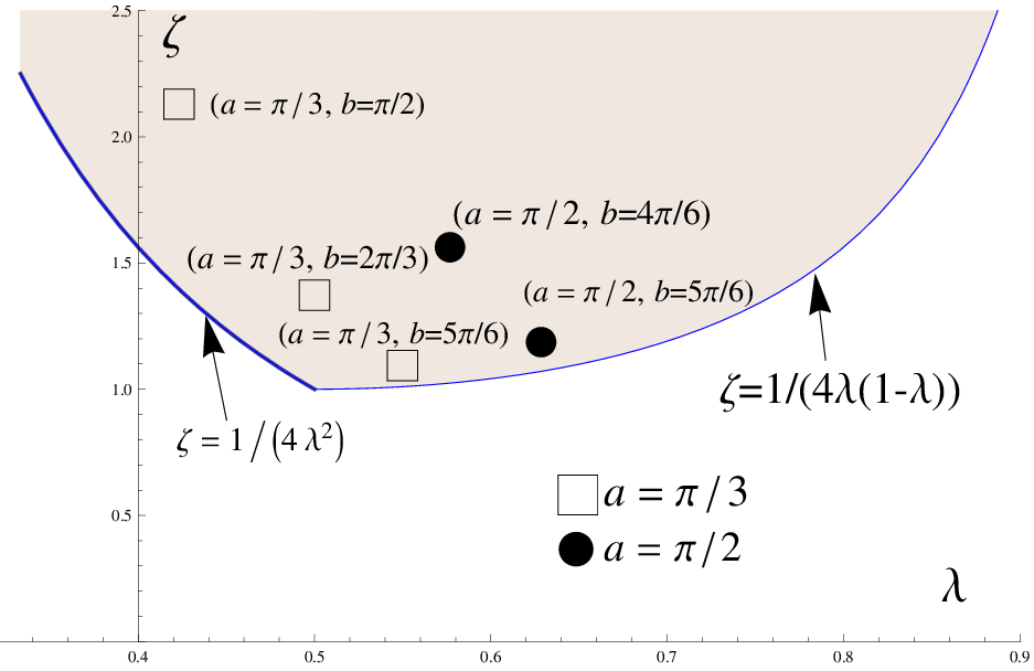

With fixed , let us consider the one parameter line with parameter in the plane. (See Fig.11). Since the is increasing function with respect to while is the decreasing function, behaves as the decreasing function with respect to . The is divergent at
| (260) |
In the fixed case, we can also consider the one parameter line with parameter in the plane. In the case of fixed , the one parameter line is represented as
| (261) |
On the other hand, in the case of fixed , the one parameter line is represented as the
| (262) |
Next let us consider the line with fixed . In this case, due to and , we can see that
| (263) |
for . Then the lines are located on the inside of the region when . Also for the case , we can show that the lines are located on the inside of the region . To show it, we should note that the value of is uniquely determined if we specify the 2 parameter . This means that there are not any intersection between two lines, and with fixed . In particular, there is no intersection of line and the , which is written as . For the lines with fixed , it becomes
| (264) |
So for , the line must be located inside the since the line can not have the intersection with the line . 4949 49 For the line with we do not have to worry about the region with . Because the range of the of the line is . This shows that two gap solution exists if and only if and . Our numerical result also shows it. (See Fig.10)
Appendix D Level-rank duality of the saddle point equation in the multi trace potential
We consider the multi-trace potential,
| (265) |
The corresponding potential in the dual theory is obtained by ,
| (266) |
Derivative of the potentials with respect to an eigenvalue are
| (267) | |||||
| (268) |
In (267), please note that only the factor carries the label dependence of the (there is no longer label dependence in the because it is the sum over the label). Similarly, in (268), the label dependence in is carried only by the factor . Saddle point equations are obtained for each eigenvalue by taking the derivative as,
| (269) | |||||
| (270) |
Now let us consider the large limit in the original theory. When we take the large limit, we first fix the residual Weyl permutation, exchanging the order of the eigenvalues. After fixing the Weyl permutation, the order of the eigenvalues obey following
| (271) |
Then there is a one to one relationship between the value of the eigenvalue and the label such that
| (272) |
In the large limit, these labels can be regarded as the continuum variable . Moreover due to the (272), becomes the increasing continuum function with respect to , so
| (273) |
And from these facts, the trace is written by the integration over the as,
| (274) |
From (273), we would like to emphasize that value of eigenvalue variable represents the label of the eigenvalue in the discretized representation. According to these, is just a large representation of the with ,
| (275) |
So, with keeping in mind that the variable represents the label of eigenvalue, becomes the with the label such that ,
This is also the case in the dual theory. At the large limit, is
with .
Now let us return to the large limit of the saddle point equation and the discussion of the level-rank duality. The large (or large ) representation of the saddle point equations are
| (278) | |||||
| (279) |
As we did from (98) to (101) in the subsection 5.2, assuming that is the solution of the (278), following
| (280) |
is a solution of the (279) for the dual theory if
| (281) |
is satisfied with (280). Then we only have to show that (281) is satisfied with (280). We can check the statement (281) directly. From (), by substituting (280), we can check
| (282) | |||||
Comparing (282) with the (), we can see (281) is satisfied with (280).
Then this concludes the proof of the level-rank duality of the saddle point equation in the multi-trace potential terms.
Appendix E High temperature limit of the partition function of a gas of non renormalized multitrace operators
In this appendix we compute the partition function of a gas of non renormalized multitrace operators, in the high temperature limit, for the theory of regular bosons, regular fermions and the supersymmetric theory with a single chiral multiplet in the fundamental representation.
The single letter partition function for bosonic theory is given by
| (283) |
where In the large temperature limit we obtain
| (284) |
The multi-trace partition function is given by
| (285) |
which in the large temperature limit is given by
| (286) |
in (286) gives the value of partition function for the gas of multi-trace operators of free bosons on the sphere of volume
For the fermionic theory, the single letter partition function is given by
| (287) |
where In the large temperature limit we obtain
| (288) |
The multi-trace partition function is given by
| (289) |
which in the large temperature limit is given by
| (290) |
which is same as that of boson obtained in (286). in (290) gives the value of partition function for the gas of multitrace operators of free fermions on the sphere of volume
For the supersymmetric theory with a chiral multiplet, the multitrace partition function is given by
| (291) |
which in the large temperature limit is given by
| (292) |
in (292) gives the value of partition function for free supersymmetric theory with a chiral multiplet on the sphere of volume This exactly matches with first term in (125).
References
- [1] E. Witten, Anti-de Sitter space, thermal phase transition, and confinement in gauge theories, Adv.Theor.Math.Phys. 2 (1998) 505–532, [hep-th/9803131].
- [2] O. Aharony, J. Marsano, S. Minwalla, K. Papadodimas, and M. Van Raamsdonk, The Hagedorn - deconfinement phase transition in weakly coupled large N gauge theories, Adv.Theor.Math.Phys. 8 (2004) 603–696, [hep-th/0310285].
- [3] L. Alvarez-Gaume, C. Gomez, H. Liu, and S. Wadia, Finite temperature effective action, AdS(5) black holes, and 1/N expansion, Phys.Rev. D71 (2005) 124023, [hep-th/0502227].
- [4] L. Alvarez-Gaume, P. Basu, M. Marino, and S. R. Wadia, Blackhole/String Transition for the Small Schwarzschild Blackhole of AdS(5)x S**5 and Critical Unitary Matrix Models, Eur.Phys.J. C48 (2006) 647–665, [hep-th/0605041].
- [5] B. Sundborg, The Hagedorn transition, deconfinement and N=4 SYM theory, Nucl.Phys. B573 (2000) 349–363, [hep-th/9908001].
- [6] O. Aharony, J. Marsano, S. Minwalla, K. Papadodimas, and M. Van Raamsdonk, A First order deconfinement transition in large N Yang-Mills theory on a small S**3, Phys.Rev. D71 (2005) 125018, [hep-th/0502149].
- [7] O. Aharony, J. Marsano, and M. Van Raamsdonk, Two loop partition function for large N pure Yang-Mills theory on a small S**3, Phys.Rev. D74 (2006) 105012, [hep-th/0608156].
- [8] K. Papadodimas, H.-H. Shieh, and M. Van Raamsdonk, A Second order deconfinement transition for large N 2+1 dimensional Yang-Mills theory on a small two-sphere, JHEP 0704 (2007) 069, [hep-th/0612066].
- [9] M. Mussel and R. Yacoby, The 2-loop partition function of large N gauge theories with adjoint matter on S**3, JHEP 0912 (2009) 005, [arXiv:0909.0407].
- [10] D. Gross and E. Witten, Possible Third Order Phase Transition in the Large N Lattice Gauge Theory, Phys.Rev. D21 (1980) 446–453.
- [11] S. R. Wadia, A Study of U(N) Lattice Gauge Theory in 2-dimensions, arXiv:1212.2906.
- [12] S. R. Wadia, N = infinity phase transition in a class of exactly soluble model lattice gauge theories, Phys.Lett. B93 (1980) 403.
- [13] R. D. Pisarski and S. Rao, Topologically Massive Chromodynamics in the Perturbative Regime, Phys.Rev. D32 (1985) 2081.
- [14] W. Chen, G. W. Semenoff, and Y.-S. Wu, Two loop analysis of nonAbelian Chern-Simons theory, Phys.Rev. D46 (1992) 5521–5539, [hep-th/9209005].
- [15] S. H. Shenker and X. Yin, Vector Models in the Singlet Sector at Finite Temperature, arXiv:1109.3519.
- [16] S. Giombi, S. Minwalla, S. Prakash, S. P. Trivedi, S. R. Wadia, et. al., Chern-Simons Theory with Vector Fermion Matter, Eur.Phys.J. C72 (2012) 2112, [arXiv:1110.4386].
- [17] C.-M. Chang, S. Minwalla, T. Sharma, and X. Yin, ABJ Triality: from Higher Spin Fields to Strings, arXiv:1207.4485.
- [18] O. Aharony, G. Gur-Ari, and R. Yacoby, d=3 Bosonic Vector Models Coupled to Chern-Simons Gauge Theories, JHEP 1203 (2012) 037, [arXiv:1110.4382].
- [19] J. Maldacena and A. Zhiboedov, Constraining Conformal Field Theories with A Higher Spin Symmetry, arXiv:1112.1016.
- [20] J. Maldacena and A. Zhiboedov, Constraining conformal field theories with a slightly broken higher spin symmetry, arXiv:1204.3882.
- [21] S. Banerjee, S. Hellerman, J. Maltz, and S. H. Shenker, Light States in Chern-Simons Theory Coupled to Fundamental Matter, arXiv:1207.4195.
- [22] O. Aharony, G. Gur-Ari, and R. Yacoby, Correlation Functions of Large N Chern-Simons-Matter Theories and Bosonization in Three Dimensions, arXiv:1207.4593.
- [23] S. Jain, S. P. Trivedi, S. R. Wadia, and S. Yokoyama, Supersymmetric Chern-Simons Theories with Vector Matter, JHEP 1210 (2012) 194, [arXiv:1207.4750].
- [24] S. Yokoyama, Chern-Simons-Fermion Vector Model with Chemical Potential, arXiv:1210.4109.
- [25] S. Banerjee, A. Castro, S. Hellerman, E. Hijano, A. Lepage-Jutier, et. al., Smoothed Transitions in Higher Spin AdS Gravity, arXiv:1209.5396.
- [26] G. Gur-Ari and R. Yacoby, Correlators of Large N Fermionic Chern-Simons Vector Models, arXiv:1211.1866.
- [27] O. Aharony, S. Giombi, G. Gur-Ari, J. Maldacena, and R. Yacoby, The Thermal Free Energy in Large N Chern-Simons-Matter Theories, arXiv:1211.4843.
- [28] A. Kapustin, B. Willett, and I. Yaakov, Nonperturbative Tests of Three-Dimensional Dualities, JHEP 1010 (2010) 013, [arXiv:1003.5694].
- [29] A. Kapustin, B. Willett, and I. Yaakov, Tests of Seiberg-like Duality in Three Dimensions, arXiv:1012.4021.
- [30] O. Aharony, G. Gur-Ari, and R. Yacoby unpublished.
- [31] F. Benini, C. Closset, and S. Cremonesi, Comments on 3d Seiberg-like dualities, JHEP 1110 (2011) 075, [arXiv:1108.5373].
- [32] M. Blau and G. Thompson, Derivation of the Verlinde formula from Chern-Simons theory and the G/G model, Nucl.Phys. B408 (1993) 345–390, [hep-th/9305010].
- [33] M. R. Douglas and V. A. Kazakov, Large N phase transition in continuum QCD in two-dimensions, Phys.Lett. B319 (1993) 219–230, [hep-th/9305047].
- [34] X. Arsiwalla, R. Boels, M. Marino, and A. Sinkovics, Phase transitions in q-deformed 2-D Yang-Mills theory and topological strings, Phys.Rev. D73 (2006) 026005, [hep-th/0509002].
- [35] N. Caporaso, M. Cirafici, L. Griguolo, S. Pasquetti, D. Seminara, et. al., Topological strings and large N phase transitions. I. Nonchiral expansion of q-deformed Yang-Mills theory, JHEP 0601 (2006) 035, [hep-th/0509041].
- [36] D. Jafferis and J. Marsano, A DK phase transition in q-deformed Yang-Mills on S**2 and topological strings, hep-th/0509004.
- [37] E. Witten, Quantum Field Theory and the Jones Polynomial, Commun.Math.Phys. 121 (1989) 351.
- [38] S. Corley, A. Jevicki, and S. Ramgoolam, Exact correlators of giant gravitons from dual N=4 SYM theory, Adv.Theor.Math.Phys. 5 (2002) 809–839, [hep-th/0111222].
- [39] C. Musili, Representations of Finite Groups, section 5.9.3, page 182 (1992).
- [40] M. R. Douglas, Chern-Simons-Witten theory as a topological Fermi liquid, hep-th/9403119.
- [41] G. ’t Hooft, Topology of the Gauge Condition and New Confinement Phases in Nonabelian Gauge Theories, Nucl.Phys. B190 (1981) 455.
- [42] G. Grignani, L. Griguolo, N. Mori, and D. Seminara, Thermodynamics of theories with sixteen supercharges in non-trivial vacua, JHEP 0710 (2007) 068, [arXiv:0707.0052].
- [43] T. Takimi, Duality and Higher Temperature Phases of Large Chern-Simons Matter Theories on , arXiv:1304.3725.
- [44] A. Kapustin, B. Willett, and I. Yaakov, Exact Results for Wilson Loops in Superconformal Chern-Simons Theories with Matter, JHEP 1003 (2010) 089, [arXiv:0909.4559].
- [45] M. A. Vasiliev, Consistent equation for interacting gauge fields of all spins in (3+1)-dimensions, Phys.Lett. B243 (1990) 378–382.
- [46] M. Vasiliev, Nonlinear equations for symmetric massless higher spin fields in (A)dS(d), Phys.Lett. B567 (2003) 139–151, [hep-th/0304049].
- [47] S. Giombi and X. Yin, The Higher Spin/Vector Model Duality, arXiv:1208.4036.