On the way of understanding the early universe cosmology, the inflationary mechanism has been proven to be quite fascinating as it successfully addresses several outstanding issues of the standard big bang scenario, e.g. the horizon problem, the flatness problem and the monopole problem. Initially, the idea of inflation was introduced to explain the homogeneous and isotropic nature of the universe at large scale structure [1, 2], however its best advantage is being utilized in studying the inhomogeneities and anisotropies of the universe, which is a consequence of the vacuum fluctuations of the inflaton (as well as the metric fluctuations). In this regard, the idea of inflation also provides a way to understand the physics which could be responsible for generating the correct amount of primordial density perturbations initiating the structure formation of the universe and the cosmic microwave background (CMB) anisotropies. The simplest (single-field) inflationary process can be understood via a (single) scalar field slowly rolling towards its in a nearly flat potential. The vacuum fluctuations of the inflaton result in an almost scale invariant spectrum with a small tilt reflecting unique predictions via the CMB radiation. Although the single-field inflationary models fit well with the current observation constraints [3, 4], the present observational data is not sufficient to discriminate among the various models. In this regard, the detection of non-Gaussianity can be a crucial data to distinguish the various models in the ongoing/future experiments such as PLANCK [5, 6, 7, 8].

In the context of string cosmology, inflationary model building have been started quite early in [9]. Since string framework can provide several flat-directions (moduli), it is promising for the embedding of inflationary scenarios in string theory. The main requirement for this purpose is to identify a scalar which could play the role of the inflaton field, i.e. its effective scalar potential has to admit a slow-roll region. In this respect, those “moduli” that have a flat potential at leading order and only by a sub-leading effect receive their dominant contribution are of interest. The perturbative effects [10, 11] as well as the instanton effects [12, 13] are proven to be extremely crucial,F especially for moduli stabilization purpose. As far as cosmological model building is concerned, the string inspired models could be given the hallmark of being ‘(semi)realistic’ only after all the moduli could be stabilized and de-Sitter solutions be realized in [14]. Since then several dS realizing mechanisms have been developed in type IIB framework [15, 16, 17, 18, 19, 20]. With the present understanding, it is fair to say that the moduli stabilization is quite well (and relatively much better) understood in type IIB orientifold models with the mechanisms like KKLT [14], Racetrack [21, 22] and the LARGE volume scenarios [23]. Significant amount of progress has been made in building up inflationary models in type IIB orientifold setups with the inflaton field identified as an open string modulus [24, 25, 26, 27] or a closed string modulus [28, 29, 30, 31, 32]. Along the lines of moduli getting lifted by sub-dominant contributions, recently so-called poly-instanton corrections became of interest. These are sub-leading non-perturbative contributions which can be briefly described as instanton corrections to instanton actions. In the recent work [33], we have clarified the zero mode conditions for an Euclidean D3-brane instanton, wrapping a divisor of the threefold, to generate such a poly-instanton effect. Utilizing the poly-instanton effects, moduli stabilization and inflation have been studied in a series of papers [32, 34, 35, 36]. Meanwhile, the studies made in the context of axionic inflationary models in the type IIB orientifold framework have been quite promising too [21, 37, 38, 39, 40, 41, 42, 43]. In [44], inflation has been realized by a combination of the brane-motion and an axion while in [45, 46, 47],, it has been driven by a combination of a (divisor) volume mode and an axion.

The signatures of non-Gaussianities are encoded in non-linearity parameters $f_{NL}$ (and $\tau_{NL}$) which parametrize the bispectrum (and trispectrum) and could be the direct evidence for detecting the non-Gaussianities. In fact, an observation of order one values for $f_{NL}$ would rules out (most of) the single field inflationary models ³³ 3 There has been some proposals of single-field models with large $f_{NL}$ values [48, 49, 50, 51].. and thus can be a potential discriminator towards picking up a more promising one. This boosts up the motivation for the study of non-Gaussianties in recent years, although it has been initiated very early [52]. A review on initial attempts regarding $f_{NL}$ computations along with observational constraints can be found in [5]. In the standard single-field models, the $f_{NL}$ parameter is usually suppressed by slow-roll parameters ($\epsilon,\eta$), e.g. $f_{NL}=n_{s}-1$ has been reported in [52]. Subsequently, the multi-field inflationary models started getting significant attention but large $f_{NL}$ could not be realize in the initial attempts [53, 54, 55, 56]. For generating observable non-Gaussianities, enormous amount of work has been done in recent couple of years and several explicit multi-field models with large $f_{NL}$ values have been found. These multi-field models can be categorized to be of separable and non-separable types.

For the separable type models, either the inflationary potential [53, 54, 55, 57, 58] or the Hubble rate [59, 60] is of sum or product separable form, and several models are available now which can produce large non-Gaussianities ⁴⁴ 4 A nice recent review about generating large non-Gaussianities for separable type setups can be found in [61, 62].. The possibilities of generating detectable large values of $f_{NL}$ during the evolution of two-fields within the slow-roll region has been proposed in [63, 64, 65]. In these models, non-Gaussianities are generated after horizon exit and consist of non-adiabatic perturbation modes. It implies such non-Gaussianities to be of local-type and hence distinguishable from the other shapes of non-Gaussianity which are realized during horizon exit [66, 67].

Unlike the separable type models, the non-Gaussianities issues in the non-separable type of potential are relatively less studied. In [56, 68, 69], a concise analytic formula for computing the non-linear parameter for a given generic multi-field potential has been developed for both the slow-roll region and beyond slow-roll region. The possibility of generating large non-Gaussianity parameter has been shown by ‘momentarily’ violating the slow-roll conditions. Following the ideas developed in [68], order one values of the $f_{NL}$ parameter has been reported in the beyond slow-roll region for a two-field large volume axionic setup [70]. Recently, some examples with (non-)separable multifield potentials have been studied in [71] which can produce large detectable values for the non-linear parameter $f_{NL}$ and $\tau_{NL}$. Higher order correction to the non-linearity parameters have been studied in [72, 73, 74, 75].

In the framework of type IIB orientifolds, several single/multi-field models have been studied for aspects of non-Gaussianities. The curvaton scenarios have been proposed in [76] for the Kähler moduli inflation setup in the context of LARGE volume scenarios. A case study have been performed in [77] for a blow-up multi-field inflationary setup (resulting in $f_{NL}\sim 0.01$) and a curvaton scenario (resulting in large $f_{NL}$ values). Later on, detectable large values of $f_{NL}$ have also been proposed via the modulated reheating mechanism in [36]. The computation of non-Gaussianties in racetrack models has been made in [78] and within the framework of KKLT-like setup, a two-field inflationary model has been proposed with inflaton dynamics governed by the Calabi Yau volume mode and the respective $C_{4}$ axion which complexifies the divisor volume mode [45]. This idea has been extended in the context of LARGE volume scenarios by generalizing the Kähler moduli (blow-up) inflation with inclusion of the corresponding $C_{4}$ axion in [46, 47]. The presence of various types of trajectories resulting in 60 (or more) number of e-foldings have been reported in this so-called “Roulette inflation” model and a subsequent investigation of non-Gaussianities in such a setup has been made in [79] resulting in small values of the $f_{NL}$ parameter.

In this article, we present a systematic analysis for a two-field inflationary model driven by a combination of a Wilson divisor volume modulus and an axion modulus in the Poly-instanton setup. The so-called Wilson divisor has a single non-trivial Wilson line modulino and is relevant for generating poly-instanton contributions which will be summarized in Section 2. For analyzing the non-Gaussianities, we proceed with the formalism developed in [68, 69] which is valid for a given generic multi-field potential in beyond slow-roll region also. We find that although the non-linearity parameters are quite small during the slow-roll regime, the same are significantly enhanced in the beyond slow-roll regime. The two-field dynamics is such that the non-linearity parameters ($f_{NL},\tau_{NL}$ and $g_{NL}$) do not get frozen at the horizon exit and keep evolving up to the end of inflation where it acquires a large value. Here, we stress that following the motion/decay of inflaton fields after the end of inflation and addressing reheating issues etc. can be extremely crucial in such models. However, the same is beyond the scope of the present analysis, and for the time being we assume that the respective values for these non-linearity parameters realized at the end of inflation do not change significantly before and by the reheating process.

The article is organized as follows. In Section 2, we start with a brief review of the relevant background about the poly-instanton setup [33] and the related moduli stabilization part [32]. In Section 3, we generalize the single field poly-instanton inflationary process into a two-field inflationary process with the inclusion of the corresponding $C_{4}$ axion and discuss the subsequent relevant changes in the slow-roll parameters. In Section 4, we present a detailed and systematic (numerical) analysis of evolutions of various inflationary trajectories (as well as the other physical observables) in terms of number of e-foldings. This analysis shows that there is a “Roulette” type inflation. In section 5, we investigate the possibility of generating finite/detectable values for the primordial non-Gaussianity parameters $f_{NL},\tau_{NL},g_{NL}$ and observe that although in the slow-roll region these are negligibly small, beyond it there exists the a possibility of enhancement to large values. Finally, in section 6 we give our conclusions followed by an appendix providing some of the lengthy intermediate expressions.

In this section, we collect the relevant ingredients for generating the poly-instanton corrections in a type IIB orientifold setup developed in [33] and briefly summarize the moduli stabilization mechanism discussed in [32]. Building on the same, we continue with the study of a generalized two-field inflationary process as well as with the computation of the non-linearity parameters (e.g. $f_{NL},\tau_{NL}$ and $g_{NL}$).

In all the remaining sections, we will be assuming that the heavier moduli are stabilized at their respective minimum position and we consider the effective potential for the two lighter fields ($\tau_{w}$ and $\rho_{w}$) given by (17). Furthermore, we assume that a suitable uplifting of the $AdS$ minimum to a $dS$ minimum can be processed via an appropriate mechanism (e.g. by the introduction of anti-D3 brane [14]⁷⁷ 7 For uplifting process using anti-D3 brane, there has been some sensitive issues as mentioned in [84, 85, 86]. or other mechanism like using dilaton-dependent term in superpotential [19]). Thus, the resulting inflationary potential looks like

$\displaystyle\hskip-42.67912ptV_{\rm inf}(\tau_{w},\rho_{w})=V_{\rm up}+V_{0}+e^{-a_{w}\tau_{w}}\left(\mu_{1}+\mu_{2}\,\tau_{w}\right)\,\cos(a_{w}\rho_{w})\,$

(21)

Now, we state the effective potential studied before in roulette inflation [46] which after stabilizing all but one Kähler moduli effectively looks as,

$\displaystyle V_{roulette}(\tau_{n},\rho_{n})=V_{\rm up}+V_{0}+\frac{\sqrt{\tau_{n}}\,e^{-2a_{n}\tau_{n}}}{\overline{\cal V}}+\frac{\tau_{n}\,e^{-a_{n}\tau_{n}}\,\cos(a_{n}\rho_{n})}{{\overline{\cal V}}^{2}}$

(22)

where $\tau_{n}$ is stabilized at $\overline{\tau}_{n}\sim{\rm ln}{\overline{\cal V}}$. Let us mention some important differences between the aforementioned potentials. First, the geometric origin of these two potential are different as we have explained in the previous sections. The former one comes from a Wilson divisor volume modulus while the later one comes from a blow-up volume modulus. Second, these moduli are stabilized by corrections which scales differently in terms of CY volume. Moreover, the stabilized values at the respective minimum have different volume scaling; $\overline{\tau}_{n}$ is stabilized at order ${\rm ln}\overline{\cal V}$ while $\tau_{w}$ is stabilized by eq.(20). Here, the $\overline{\cal V}$ dependence, which could have appeared via $\overline{\tau}_{s}$, gets effectively canceled.

The uplifting term $V_{\rm up}$ in eq.(21) needs to be such that the uplifted scalar potential acquires a small positive value (to be matched with the cosmological constant) when all the moduli sit at their respective minimum. This potential has the following set of critical points

	$\displaystyle(i).\hskip 28.45274pt\overline{\tau}_{w}=\frac{\mu_{2}-a_{w}\,\mu_{1}}{a_{w}\,\mu_{2}},\,\,\,a_{w}\overline{\rho}_{w}=2p\,\pi$		(23)
	$\displaystyle(ii).\hskip 25.03856pt\overline{\tau}_{w}=\frac{\mu_{2}-a_{w}\,\mu_{1}}{a_{w}\,\mu_{2}},\,\,\,a_{w}\overline{\rho}_{w}=(2p+1)\pi$

where $p\in\mathbb{Z}$. Moreover, in order to trust the effective field theory we need $\frac{\mu_{1}}{\mu_{2}}<0$. In order to ensure the minimum, one has to consider the Hessian $V_{ab}$ (evaluated at these two sets of critical points) which is given as

$\displaystyle\hskip-28.45274ptV_{ab}=\left(\begin{array}[]{ll}\mp a_{w}\,\mu_{2}\,e^{-1+\frac{a_{w}\,\mu_{1}}{\mu_{2}}}&\,\,\,\,\,\,\,\,\,\,\,\,\,0\\ \,\,\,\,\,\,\,\,\,\,\,\,\,\,\,\,0&\mp a_{w}\,\mu_{2}\,e^{-1+\frac{a_{w}\,\mu_{1}}{\mu_{2}}}\end{array}\right)\,,$

where $\mp$ sign corresponds to critical points $(i)$ and $(ii)$ respectively. Hence depending on whether $\{\mu_{1}<0,\mu_{2}>0\}$ or $\{\mu_{1}>0,\mu_{2}<0\}$, we find that one set of critical point corresponds to minima while the other corresponds to maxima. From now on, we fix our notation with a sampling of parameters such that $\{\mu_{1}>0,\mu_{2}<0\}$ (as in [32]) and performing the redefinitions $\tau_{w}=\phi_{1},\,\rho_{w}=\phi_{2}$, the uplifted scalar potential takes the form

$\displaystyle\hskip-36.98866ptV_{\rm inf}(\phi_{1},\phi_{2})=\left(\frac{g_{s}}{8\pi}\right)\,e^{K_{\rm CS}}\,\left[-\frac{\mu_{2}\,e^{-1+\frac{a_{w}\,\mu_{1}}{\mu_{2}}}}{a_{w}}+e^{-a_{w}\phi_{1}}\left(\mu_{1}+\mu_{2}\,\phi_{1}\right)\,\cos(a_{w}\phi_{2})\,\right].$

(27)

Here, a proper normalization factor $\left(\frac{g_{s}}{8\pi}\right)\,e^{K_{\rm CS}}$ has been included [28], where $K_{\rm CS}$ denotes the Kähler potential for the complex structure moduli. We assume that $e^{K_{\rm CS}}\sim{\cal O}(1)$. Furthermore, we set the numerical parameters for moduli stabilization similar to the ones chosen in one of the benchmark models (in [32]). The parameters which would be directly relevant for further computations in this article are,

	$\displaystyle\mu_{1}=2.9\times 10^{-8},\,\mu_{2}=-1.9\times 10^{-8},\,a_{w}=2\pi,g_{s}=0.12$		(28)
	$\displaystyle\hskip 56.9055pt\overline{\cal V}=905,\overline{\tau}_{s}=5.7,\xi_{sw}=1/(6\sqrt{2})$

The ‘effective’ non-flat moduli space metric ${\cal G}_{ab}$ relevant for inflaton dynamics can be computed as

$\displaystyle{\cal G}_{ab}=\left(\begin{array}[]{ll}\frac{3\xi_{sw}}{2\,\sqrt{2}\,{\cal V}\,\sqrt{{\tau_{s}}+{\phi_{1}}}}&\,\,\,\,\,\,\,\,\,\,\,\,0\\ \,\,\,\,\,\,\,\,\,\,\,\,\,0&\frac{3\xi_{sw}}{2\,\sqrt{2}\,{\cal V}\,\sqrt{{\tau_{s}}+{\phi_{1}}}}\end{array}\right)\,$

Utilizing the large volume limit, the same is written from the Kähler metric component $K_{T_{w}{\overline{T}}_{w}}$ expressed in the real moduli basis $\{\phi_{1},\phi_{2}\}$. The Christoffel connections are defined as $\Gamma^{a}_{\,\,bc}={\cal G}^{ad}\Gamma_{bc,d}=\frac{1}{2}{\cal G}^{ad}\left(\partial_{b}{\cal G}_{cd}+\partial_{c}{\cal G}_{bd}-\partial_{d}{\cal G}_{bc}\right)$ and the only non-zero connection components are

$$\Gamma_{\,\,11}^{1}=-\frac{1}{4(\overline{\tau}_{3}+\phi_{1})}=\Gamma_{\,\,12}^{2}=\Gamma_{\,\,21}^{2},\,\,\Gamma_{\,\,22}^{1}=\frac{1}{4(\overline{\tau}_{3}+\phi_{1})}.$$

Furthermore, the non-zero components of the Riemann tensor, defined as $R^{a}_{\,\,\,bcd}=\partial_{c}\Gamma^{a}_{\,\,db}-\partial_{d}\Gamma^{a}_{\,\,cb}+\Gamma^{a}_{\,\,ck}\Gamma^{k}_{\,\,db}-\Gamma^{a}_{\,\,dk}\Gamma^{k}_{\,\,cb}$, are

$$R_{\,\,212}^{1}=-\frac{1}{2(\overline{\tau}_{3}+\phi_{1})^{2}}=R_{\,\,121}^{2},\,\,R_{\,\,221}^{1}=\frac{1}{2(\overline{\tau}_{3}+\phi_{1})^{2}}=R_{\,\,112}^{2}.$$

Under the sampling (28), the effective two-field inflationary potential from eq.(21) is shown in Fig.1.

In this section, we investigate the field evolutions and look for the possible inflationary trajectories which could reproduce 50 (or more) e-foldings. For a given initial condition, we numerically trace the entire inflationary trajectories including beyond slow-roll region. Using the background $N$ e-folding number as the time coordinate, i.e. $dN=Hdt$, the Einstein-Friedmann equations are obtained as

	$\displaystyle\frac{d^{2}}{dN^{2}}\phi^{a}+{\Gamma^{a}}_{bc}\frac{d\phi^{b}}{dN}\frac{d\phi^{c}}{dN}+\left(3+\frac{1}{H}\frac{dH}{dN}\right)\frac{d\phi^{a}}{dN}+\frac{{\cal G}^{ab}\partial_{b}V}{H^{2}}=0,$		(32a)
	$\displaystyle H^{2}=\frac{1}{3}\left(V(\phi^{a})+\frac{1}{2}H^{2}\,{\cal G}_{ab}\frac{d\phi^{a}}{dN}\frac{d\phi^{b}}{dN}\right).$		(32b)

Using expressions (32a) and (32b), one can derive another useful expression for variation of Hubble rate in terms of e-folding,

$\displaystyle\frac{1}{H}\frac{dH}{dN}=\frac{V}{H^{2}}-3.$

(33)

For numerical convenience, we solve these equations in the time basis $t$ and then change the result back to the basis $N$ e-folding. As introduced in [69], we will follow the field redefinitions given as⁸⁸ 8 The use of this notation would be more clear in the next section regarding computations of non-linearity parameters. Further, we will be using a combined indexing ${\cal A}$ such that any object ${\cal O}^{\cal A}$ has two components given as ${\cal O}^{\cal A}\equiv\{{\cal O}^{a}_{1},{\cal O}^{a}_{2}\}$.

$\displaystyle\varphi^{a}_{1}\equiv\phi^{a},\,\,\,\,\,\,\ \varphi^{a}_{2}\equiv\dot{\phi}^{a}=\left(\frac{d\phi^{a}}{dt}\right),\,\,\,\,\ {\rm where}\,\,a=1,\,2.$

(34)

which translates the second-order background equations of motions eq.(32a) into two first-order ODEs as follows

	$\displaystyle F^{a}_{1}\equiv\frac{d\varphi^{a}_{1}}{dN}=\left(\frac{d\phi^{a}}{dN}\right)=\frac{\varphi^{a}_{2}}{H},$
	$\displaystyle F^{a}_{2}\equiv\frac{D\varphi^{a}_{2}}{dN}=-3\varphi^{a}_{2}-{\cal G}^{ab}\frac{V_{b}}{H}.$		(35)

where $D$ is the covariant derivative defined as $D\varphi^{a}_{2}=d\varphi^{a}_{2}+{\Gamma^{a}}_{bc}\varphi^{b}_{2}d\varphi^{c}_{1}$, subject to the constraints $H^{2}=\frac{1}{3}\left(V+\frac{1}{2}\,{\cal G}_{ab}\varphi^{a}_{2}\varphi^{b}_{2}\right)$. Then eq.(33) will be simplified as $\frac{dH}{dt}=-\frac{1}{2}\,{\cal G}_{ab}\varphi^{a}_{2}\varphi^{b}_{2}$. Now, in the context of studying inflationary aspects, one has to look at the sufficient conditions for realizing slow-roll inflation which are encoded in the so-called slow-roll parameters. For multi-field inflationary process with inflatons moving in a non-flat background, these slow-roll parameters are given as,

$\displaystyle\epsilon\equiv-\frac{1}{H^{2}}\frac{dH}{dt},\,\,\,\,\,\,\,\,\eta\equiv\frac{1}{\epsilon H}\frac{d\epsilon}{dt}.$

(36)

Now, we can solve the background field equations (35) to get the full trajectories under different initial conditions. We choose $\phi^{a}(0)=\phi^{a}_{0}\,\,{\rm and}\,\,\frac{d\phi^{a}}{dt}\frac{d\phi_{a}}{dt}|_{t=0}=0;\,\,{\rm for}\,\,a\in\{1,2\}$ as a set of initial conditions and trace the corresponding trajectories up to the end of inflation (see Table 2).Figure 2 shows the complex evolution of trajectories for some samples of general starting conditions where the value of $N$ e-folding at the end of inflation is labeled on each of these trajectories. Note, although it looks like a single field inflation in the late period of trajectory, the axion field in fact oscillates (Figure 3) during that time before settling into its minimum. The fact that both of the fields in each trajectories keep evolving up to the end of inflation might be relevant for generating large Non-Gaussianity. This indicates that isocurvature modes are not completely finished even though it looks as a single field motion in the final stage of the trajectories. The $N$ e-folding when the axion $\rho_{w}$ first crosses its minimum is denoted as $N^{\dagger}$. One has to note that at this time $N^{\dagger}$, the Wilson divisor volume mode is still quite far from its respective minimum. However, it rolls quickly enough to reach there. All of these points $N^{\dagger}$ are already in the beyond slow-roll region as the slow-roll parameter $\eta>1$.

The various inflationary trajectories shown in Figure.2 can be classified in the following categories

1. (a)

   If the axion initial condition is such that the axion is minimized at its respective minimum, then two-field inflationary process reduces to its single field analogue which has been studied in [32]. These are stable trajectories and are attracted towards the respective valley in a straight line like the trajectory in Figure.2 with $N_{F}=62$. These can produce the required number of e-foldings if the Wilson divisor volume mode is displaced significantly away from the minimum.

2. (b)

   If the axion initial condition is a little bit away from the minimum, the trajectories rolls to the nearest valley and trace towards the respective minimum like those trajectories in Figure.2 with $N_{F}=1,\,53.4,\,65,\,98.8$.

3. (c)

   If the axion initial condition starts with its value at the maximum, this results in an unstable trajectory directed straightly outwards from the respective attractor point showing a run-away behavior like the yellow trajectory in Figure.2.

4. (d)

   The trajectories starts from axion initial conditions being closer (but not exactly equal) to some maximum value as well as the initial values for the divisor volume mode being not very far from its respective minimum, one observes that inflationary trajectories cross several axion-ridges before getting attracted into a valley. This can be understood from the fact that this class of initial conditions is such that the initial potential energy is just a little higher to begin with (as shown in Figure.4 ) and the $N$ e-folding increase very slow at the beginning of these trajectories, see Figure.2 with $N_{F}=7.4,\,44.2,\,270$.

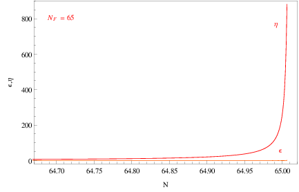
For most of these trajectories except the single-field one, they momentarily undergo some sort of quick-roll region before staring the slow-roll (see Figure 4, 5 and 6). The slow-roll region ends when any of the slow roll conditions $\epsilon\ll 1,\,\eta\ll 1$ is violated. The evolution of the slow-roll parameter $\epsilon$ and $\eta$ depending on the variation of e-folding for four of these trajectories are shown in Figure 5 from which one can see that these parameter changes dramatically at the end of inflation. Also, there is a region in field space where there is a strong violation of slow-roll condition via $\eta\gg 1$ before the end of inflation. This beyond slow-roll region can be interesting from the non-Gaussianities point of view as explained later. Furthermore, we can define the scalar perturbation power spectrum $P_{s}$ (in the slow-roll region) as $P_{s}=\frac{H^{2}}{(2\pi)^{2}\epsilon}$. Figure 6 shows the evolution of the Hubble rate $H$ and power spectrum $P_{s}$ with e-folding variations for the corresponding trajectories. It shows that the Hubble rate $H$ is almost constant (at $10^{-8}M_{p}$) during entire inflationary process including the beyond slow-roll region also. This indicates a high scale inflation as $M_{\rm inf}\sim V_{\rm inf}^{\frac{1}{4}}\sim H^{\frac{1}{2}}\sim 10^{14}$GeV. The power spectrum for scalar perturbations $P_{s}$ reaches a value of order $10^{-9}$ at the horizon exit. Also, within the slow-roll limit, the spectral index is found to be negligibly small. All of these results are consistent with the observational constraints today.

The signatures of non-Gaussianities are encoded in a set of non-linearity parameters which are commonly denoted as $f_{NL},\tau_{NL}$ and $g_{NL}$. These are generically related to the n-point correlators of curvature perturbations; the 2-point correlators simply give rise to a Gaussian shaped power spectrum while the 3-point correlators are related to the bi-spectrum which encodes the non-Gaussianities via the non-linearity parameter $f_{NL}$. Similarly, the 4-point correlators give rise to a tri-spectrum via $\tau_{NL}$ and $g_{NL}$ parameters. These non-linearity parameters can be computed in the $\delta N$-formalism which relates the curvature perturbations to the difference between the number of e-foldings $\delta N$ of two constant time-hypersurfaces [52],

$$\zeta(t,x)\simeq\delta N=H\delta t$$

Following the redefinitions of the background field evolutions as made in the previous section, the perturbations of the scalar field on $N={\rm constant}$ gauge can be expressed as,

$$\delta\varphi^{\cal A}(\lambda,N)\equiv\varphi^{\cal A}(\lambda+\delta\lambda,N)-\varphi^{\cal A}(\lambda,N)$$

where $\lambda$’s are $2{n}-1$ integration constants (for an $n$- component scalar field) which, along with $N$, parametrizes the initial values of the fields [68, 69]. The curvature perturbations at each spatial point of the field space are subsequently expressed in terms of variations of the number of e-foldings in various field directions,

	$\displaystyle\zeta(N_{F},{\bf x})=\sum\frac{1}{n!}N^{*}_{{\cal A}_{1}{\cal A}_{2}....{\cal A}_{n}}\,\delta\varphi^{{\cal A}_{1}}({\bf x})\,\delta\varphi^{{\cal A}_{2}}({\bf x})......\delta\varphi^{{\cal A}_{n}}({\bf x}),$		(37)
	$\displaystyle\hskip-8.5359ptN^{*}_{{\cal A}_{1}{\cal A}_{2}....{\cal A}_{n}}\equiv\left(\frac{\partial^{n}N(N_{F},{\varphi^{\cal A}})}{\partial\varphi^{{\cal A}_{1}}\partial\varphi^{{\cal A}_{2}}....\partial\varphi^{{\cal A}_{n}}}\right)_{at\,\,\,\varphi^{\cal A}=\varphi^{\cal A}_{(0)}(N_{*})}$

where $\varphi^{\cal A}_{(0)}$ corresponds to an unperturbed trajectory and $N_{F}$ corresponds to a final time-hypersurface of uniform energy density. The non-linearity parameters $f_{NL}$, $\tau_{NL}$ and $g_{NL}$ are generically defined as,

	$\displaystyle f_{NL}=\frac{5}{6}\,\frac{N^{\cal A}\,N^{\cal B}\,N_{{\cal A}{\cal B}}}{(N^{\cal D}\,N_{\cal D})^{2}},$
	$\displaystyle\tau_{NL}=\,\frac{N^{\cal A}\,N_{{\cal A}{\cal B}}\,N^{{\cal B}{\cal C}}\,N_{\cal C}}{(N^{\cal D}\,N_{\cal D})^{3}},$		(38)
	$\displaystyle g_{NL}=\frac{25}{54}\,\frac{N^{\cal A}\,N^{\cal B}\,N^{\cal C}\,N_{{\cal A}{\cal B}{\cal C}}}{(N^{\cal D}\,N_{\cal D})^{3}}$

where the field variations of $N$ are defined as $N_{\cal A}=\partial_{\cal A}N,N_{{\cal A}{\cal B}}=\partial_{{\cal A}{\cal B}}N$ and $N^{\cal A}={\cal G}^{{\cal A}{\cal B}}N_{\cal B}$. Now, the main task in computing the non-linearity parameters is to find out the fields variations of the number of e-foldings and for the same we would follow the strategy developed in [68, 69] using $\delta N$ formalism. It is important to mention that this approach is valid in the beyond slow-roll regime as well. So one can explore the evolutions of the non-linearity parameter in the non slow-roll regime up to the end of inflation.

References

- [1] A. H. Guth, “The Inflationary Universe: A Possible Solution to the Horizon and Flatness Problems,” Phys. Rev. D23 (1981) 347–356.
- [2] A. D. Linde, “A New Inflationary Universe Scenario: A Possible Solution of the Horizon, Flatness, Homogeneity, Isotropy and Primordial Monopole Problems,” Phys. Lett. B108 (1982) 389–393.
- [3] D. Larson, J. Dunkley, G. Hinshaw, E. Komatsu, M. Nolta, et al., “Seven-Year Wilkinson Microwave Anisotropy Probe (WMAP) Observations: Power Spectra and WMAP-Derived Parameters,” Astrophys.J.Suppl. 192 (2011) 16, 1001.4635.
- [4] WMAP Collaboration, E. Komatsu et al., “Seven-Year Wilkinson Microwave Anisotropy Probe (WMAP) Observations: Cosmological Interpretation,” Astrophys.J.Suppl. 192 (2011) 18, 1001.4538.
- [5] N. Bartolo, E. Komatsu, S. Matarrese, and A. Riotto, “Non-Gaussianity from inflation: Theory and observations,” Phys.Rept. 402 (2004) 103–266, astro-ph/0406398.
- [6] Planck Collaboration, “The Scientific programme of planck,” astro-ph/0604069.
- [7] A. P. Yadav and B. D. Wandelt, “Evidence of Primordial Non-Gaussianity (f(NL)) in the Wilkinson Microwave Anisotropy Probe 3-Year Data at 2.8sigma,” Phys.Rev.Lett. 100 (2008) 181301, 0712.1148.
- [8] G. Efstathiou and S. Gratton, “B-mode Detection with an Extended Planck Mission,” JCAP 0906 (2009) 011, 0903.0345.
- [9] G. Dvali and S. H. Tye, “Brane inflation,” Phys.Lett. B450 (1999) 72–82, hep-ph/9812483.
- [10] K. Becker, M. Becker, M. Haack, and J. Louis, “Supersymmetry breaking and alpha-prime corrections to flux induced potentials,” JHEP 0206 (2002) 060, hep-th/0204254.
- [11] S. Gukov, C. Vafa, and E. Witten, “CFT’s from Calabi-Yau four folds,” Nucl.Phys. B584 (2000) 69–108, hep-th/9906070.
- [12] E. Witten, “Non-Perturbative Superpotentials In String Theory,” Nucl. Phys. B474 (1996) 343–360, hep-th/9604030.
- [13] R. Blumenhagen, M. Cvetic, S. Kachru, and T. Weigand, “D-Brane Instantons in Type II Orientifolds,” Ann. Rev. Nucl. Part. Sci. 59 (2009) 269–296, 0902.3251.
- [14] S. Kachru, R. Kallosh, A. D. Linde, and S. P. Trivedi, “De Sitter vacua in string theory,” Phys.Rev. D68 (2003) 046005, hep-th/0301240.
- [15] C. Burgess, R. Kallosh, and F. Quevedo, “De Sitter string vacua from supersymmetric D terms,” JHEP 0310 (2003) 056, hep-th/0309187.
- [16] A. Saltman and E. Silverstein, “The Scaling of the no scale potential and de Sitter model building,” JHEP 0411 (2004) 066, hep-th/0402135.
- [17] A. Westphal, “de Sitter string vacua from Kahler uplifting,” JHEP 0703 (2007) 102, hep-th/0611332.
- [18] A. Misra and P. Shukla, “Moduli stabilization, large-volume dS minimum without D3-bar branes, (non-)supersymmetric black hole attractors and two-parameter Swiss cheese Calabi-Yau’s,” Nucl.Phys. B799 (2008) 165–198, 0707.0105.
- [19] M. Cicoli, A. Maharana, F. Quevedo, and C. Burgess, “De Sitter String Vacua from Dilaton-dependent Non-perturbative Effects,” 1203.1750. 22 pages + two appendices, typos corrected.
- [20] J. Louis, M. Rummel, R. Valandro, and A. Westphal, “Building an explicit de Sitter,” JHEP 1210 (2012) 163, 1208.3208.
- [21] J. Blanco-Pillado, C. Burgess, J. M. Cline, C. Escoda, M. Gomez-Reino, et al., “Racetrack inflation,” JHEP 0411 (2004) 063, hep-th/0406230.
- [22] H. Abe, T. Higaki, and T. Kobayashi, “Moduli-mixing racetrack model,” Nucl.Phys. B742 (2006) 187–207, hep-th/0512232.
- [23] V. Balasubramanian, P. Berglund, J. P. Conlon, and F. Quevedo, “Systematics of moduli stabilisation in Calabi-Yau flux compactifications,” JHEP 0503 (2005) 007, hep-th/0502058.
- [24] S. Kachru, R. Kallosh, A. D. Linde, J. M. Maldacena, L. P. McAllister, et al., “Towards inflation in string theory,” JCAP 0310 (2003) 013, hep-th/0308055.
- [25] K. Dasgupta, J. P. Hsu, R. Kallosh, A. D. Linde, and M. Zagermann, “D3/D7 brane inflation and semilocal strings,” JHEP 0408 (2004) 030, hep-th/0405247.
- [26] A. Avgoustidis, D. Cremades, and F. Quevedo, “Wilson line inflation,” Gen.Rel.Grav. 39 (2007) 1203–1234, hep-th/0606031.
- [27] D. Baumann, A. Dymarsky, S. Kachru, I. R. Klebanov, and L. McAllister, “Compactification Effects in D-brane Inflation,” Phys.Rev.Lett. 104 (2010) 251602, 0912.4268.
- [28] J. P. Conlon and F. Quevedo, “Kahler moduli inflation,” JHEP 0601 (2006) 146, hep-th/0509012.
- [29] J. P. Conlon, R. Kallosh, A. D. Linde, and F. Quevedo, “Volume Modulus Inflation and the Gravitino Mass Problem,” JCAP 0809 (2008) 011, 0806.0809.
- [30] M. Cicoli, C. Burgess, and F. Quevedo, “Fibre Inflation: Observable Gravity Waves from IIB String Compactifications,” JCAP 0903 (2009) 013, 0808.0691.
- [31] M. Cicoli and F. Quevedo, “String moduli inflation: An overview,” Class.Quant.Grav. 28 (2011) 204001, 1108.2659.
- [32] R. Blumenhagen, X. Gao, T. Rahn, and P. Shukla, “Moduli Stabilization and Inflationary Cosmology with Poly-Instantons in Type IIB Orientifolds,” JHEP 1211 (2012) 101, 1208.1160.
- [33] R. Blumenhagen, X. Gao, T. Rahn, and P. Shukla, “A Note on Poly-Instanton Effects in Type IIB Orientifolds on Calabi-Yau Threefolds,” JHEP 1206 (2012) 162, 1205.2485.
- [34] R. Blumenhagen, S. Moster, and E. Plauschinn, “String GUT Scenarios with Stabilised Moduli,” Phys.Rev. D78 (2008) 066008, 0806.2667.
- [35] M. Cicoli, F. G. Pedro, and G. Tasinato, “Poly-instanton Inflation,” JCAP 1112 (2011) 022, 1110.6182.
- [36] M. Cicoli, G. Tasinato, I. Zavala, C. Burgess, and F. Quevedo, “Modulated Reheating and Large Non-Gaussianity in String Cosmology,” JCAP 1205 (2012) 039, 1202.4580.
- [37] S. Dimopoulos, S. Kachru, J. McGreevy, and J. G. Wacker, “N-flation,” JCAP 0808 (2008) 003, hep-th/0507205.
- [38] J. Blanco-Pillado, C. Burgess, J. M. Cline, C. Escoda, M. Gomez-Reino, et al., “Inflating in a better racetrack,” JHEP 0609 (2006) 002, hep-th/0603129.
- [39] R. Kallosh, N. Sivanandam, and M. Soroush, “Axion Inflation and Gravity Waves in String Theory,” Phys.Rev. D77 (2008) 043501, 0710.3429.
- [40] M. Cicoli, F. G. Pedro, and G. Tasinato, “Natural Quintessence in String Theory,” 1203.6655.
- [41] T. W. Grimm, “Axion inflation in type II string theory,” Phys.Rev. D77 (2008) 126007, 0710.3883.
- [42] A. Misra and P. Shukla, “Large Volume Axionic Swiss-Cheese Inflation,” Nucl.Phys. B800 (2008) 384–400, 0712.1260.
- [43] L. McAllister, E. Silverstein, and A. Westphal, “Gravity Waves and Linear Inflation from Axion Monodromy,” Phys.Rev. D82 (2010) 046003, 0808.0706.
- [44] C. Burgess, J. M. Cline, and M. Postma, “Axionic D3-D7 Inflation,” JHEP 0903 (2009) 058, 0811.1503.
- [45] R. Kallosh and S. Prokushkin, “SuperCosmology,” hep-th/0403060.
- [46] J. R. Bond, L. Kofman, S. Prokushkin, and P. M. Vaudrevange, “Roulette inflation with Kahler moduli and their axions,” Phys.Rev. D75 (2007) 123511, hep-th/0612197.
- [47] J. J. Blanco-Pillado, D. Buck, E. J. Copeland, M. Gomez-Reino, and N. J. Nunes, “Kahler Moduli Inflation Revisited,” JHEP 1001 (2010) 081, 0906.3711.
- [48] T. Qiu and K.-C. Yang, “Non-Gaussianities of Single Field Inflation with Non-minimal Coupling,” Phys.Rev. D83 (2011) 084022, 1012.1697.
- [49] M. H. Namjoo, H. Firouzjahi, and M. Sasaki, “Violation of non-Gaussianity consistency relation in a single field inflationary model,” 1210.3692.
- [50] J. Noller and J. Magueijo, “Non-Gaussianity in single field models without slow-roll,” Phys.Rev. D83 (2011) 103511, 1102.0275.
- [51] K. T. Engel, K. S. Lee, and M. B. Wise, “Trispectrum versus Bispectrum in Single-Field Inflation,” Phys.Rev. D79 (2009) 103530, 0811.3964.
- [52] J. M. Maldacena, “Non-Gaussian features of primordial fluctuations in single field inflationary models,” JHEP 0305 (2003) 013, astro-ph/0210603.
- [53] F. Vernizzi and D. Wands, “Non-gaussianities in two-field inflation,” JCAP 0605 (2006) 019, astro-ph/0603799.
- [54] T. Battefeld and R. Easther, “Non-Gaussianities in Multi-field Inflation,” JCAP 0703 (2007) 020, astro-ph/0610296.
- [55] K.-Y. Choi, L. M. Hall, and C. van de Bruck, “Spectral Running and Non-Gaussianity from Slow-Roll Inflation in Generalised Two-Field Models,” JCAP 0702 (2007) 029, astro-ph/0701247.
- [56] S. Yokoyama, T. Suyama, and T. Tanaka, “Primordial Non-Gaussianity in Multi-Scalar Slow-Roll Inflation,” JCAP 0707 (2007) 013, 0705.3178.
- [57] G. Rigopoulos, E. Shellard, and B. van Tent, “Quantitative bispectra from multifield inflation,” Phys.Rev. D76 (2007) 083512, astro-ph/0511041.
- [58] D. Seery and J. E. Lidsey, “Non-Gaussianity from the inflationary trispectrum,” JCAP 0701 (2007) 008, astro-ph/0611034.
- [59] C. T. Byrnes and G. Tasinato, “Non-Gaussianity beyond slow roll in multi-field inflation,” JCAP 0908 (2009) 016, 0906.0767.
- [60] D. Battefeld and T. Battefeld, “On Non-Gaussianities in Multi-Field Inflation (N fields): Bi and Tri-spectra beyond Slow-Roll,” JCAP 0911 (2009) 010, 0908.4269.
- [61] C. T. Byrnes and K.-Y. Choi, “Review of local non-Gaussianity from multi-field inflation,” Adv.Astron. 2010 (2010) 724525, 1002.3110.
- [62] T. Suyama, T. Takahashi, M. Yamaguchi, and S. Yokoyama, “On Classification of Models of Large Local-Type Non-Gaussianity,” JCAP 1012 (2010) 030, 1009.1979.
- [63] C. T. Byrnes, K.-Y. Choi, and L. M. Hall, “Conditions for large non-Gaussianity in two-field slow-roll inflation,” JCAP 0810 (2008) 008, 0807.1101.
- [64] C. T. Byrnes, “Constraints on generating the primordial curvature perturbation and non-Gaussianity from instant preheating,” JCAP 0901 (2009) 011, 0810.3913.
- [65] C. T. Byrnes, K.-Y. Choi, and L. M. Hall, “Large non-Gaussianity from two-component hybrid inflation,” JCAP 0902 (2009) 017, 0812.0807.
- [66] E. Komatsu, N. Afshordi, N. Bartolo, D. Baumann, J. Bond, et al., “Non-Gaussianity as a Probe of the Physics of the Primordial Universe and the Astrophysics of the Low Redshift Universe,” 0902.4759.
- [67] J. Fergusson and E. Shellard, “The shape of primordial non-Gaussianity and the CMB bispectrum,” Phys.Rev. D80 (2009) 043510, 0812.3413.
- [68] S. Yokoyama, T. Suyama, and T. Tanaka, “Primordial Non-Gaussianity in Multi-Scalar Inflation,” Phys.Rev. D77 (2008) 083511, 0711.2920.
- [69] S. Yokoyama, T. Suyama, and T. Tanaka, “Efficient diagrammatic computation method for higher order correlation functions of local type primordial curvature perturbations,” JCAP 0902 (2009) 012, 0810.3053.
- [70] A. Misra and P. Shukla, “’Finite’ Non-Gaussianities and Tensor-Scalar Ratio in Large Volume Swiss-Cheese Compactifications,” Nucl.Phys. B810 (2009) 174–192, 0807.0996.
- [71] A. Mazumdar and L.-F. Wang, “Separable and non-separable multi-field inflation and large non-Gaussianity,” JCAP 1209 (2012) 005, 1203.3558.
- [72] D. H. Lyth and Y. Rodriguez, “The Inflationary prediction for primordial non-Gaussianity,” Phys.Rev.Lett. 95 (2005) 121302, astro-ph/0504045.
- [73] I. Zaballa, Y. Rodriguez, and D. H. Lyth, “Higher order contributions to the primordial non-Gaussianity,” JCAP 0606 (2006) 013, astro-ph/0603534.
- [74] H. R. Cogollo, Y. Rodriguez, and C. A. Valenzuela-Toledo, “On the Issue of the zeta Series Convergence and Loop Corrections in the Generation of Observable Primordial Non-Gaussianity in Slow-Roll Inflation. Part I: The Bispectrum,” JCAP 0808 (2008) 029, 0806.1546.
- [75] Y. Rodriguez and C. A. Valenzuela-Toledo, “On the Issue of the zeta Series Convergence and Loop Corrections in the Generation of Observable Primordial Non-Gaussianity in Slow-Roll Inflation. Part 2. The Trispectrum,” Phys.Rev. D81 (2010) 023531, 0811.4092.
- [76] C. Burgess, M. Cicoli, M. Gomez-Reino, F. Quevedo, G. Tasinato, et al., “Non-standard primordial fluctuations and nongaussianity in string inflation,” JHEP 1008 (2010) 045, 1005.4840.
- [77] P. Berglund and G. Ren, “Non-Gaussianity in String Cosmology: A Case Study,” 1010.3261.
- [78] C.-Y. Sun and D.-H. Zhang, “The Non-Gaussianity of Racetrack Inflation Models,” Commun.Theor.Phys. 48 (2007) 189–192, astro-ph/0604298.
- [79] A. C. Vincent and J. M. Cline, “Curvature Spectra and Nongaussianities in the Roulette Inflation Model,” JHEP 0810 (2008) 093, 0809.2982.
- [80] R. Blumenhagen and M. Schmidt-Sommerfeld, “Power Towers of String Instantons for N=1 Vacua,” JHEP 0807 (2008) 027, 0803.1562.
- [81] C. Petersson, P. Soler, and A. M. Uranga, “D-instanton and polyinstanton effects from type I’ D0-brane loops,” JHEP 1006 (2010) 089, 1001.3390.
- [82] M. Grana, “Flux compactifications in string theory: A Comprehensive review,” Phys.Rept. 423 (2006) 91–158, hep-th/0509003.
- [83] R. Blumenhagen, B. Kors, D. Lust, and S. Stieberger, “Four-dimensional String Compactifications with D-Branes, Orientifolds and Fluxes,” Phys.Rept. 445 (2007) 1–193, hep-th/0610327.
- [84] J. Blaback, U. H. Danielsson, and T. Van Riet, “Resolving anti-brane singularities through time-dependence,” 1202.1132.
- [85] I. Bena, M. Grana, S. Kuperstein, and S. Massai, “Polchinski-Strassler does not uplift Klebanov-Strassler,” 1212.4828.
- [86] I. Bena, M. Grana, S. Kuperstein, and S. Massai, “Anti-D3’s - Singular to the Bitter End,” 1206.6369.
- [87] C. T. Byrnes, M. Sasaki, and D. Wands, “The primordial trispectrum from inflation,” Phys.Rev. D74 (2006) 123519, astro-ph/0611075.
- [88] Y.-F. Cai and H.-Y. Xia, “Inflation with multiple sound speeds: a model of multiple DBI type actions and non-Gaussianities,” Phys.Lett. B677 (2009) 226–234, 0904.0062.
- [89] T. Tanaka, T. Suyama, and S. Yokoyama, “Use of delta N formalism - Difficulties in generating large local-type non-Gaussianity during inflation -,” Class.Quant.Grav. 27 (2010) 124003, 1003.5057.
- [90] A. Mazumdar and J. Rocher, “Particle physics models of inflation and curvaton scenarios,” Phys.Rept. 497 (2011) 85–215, 1001.0993.
- [91] M. Cicoli and A. Mazumdar, “Reheating for Closed String Inflation,” JCAP 1009 (2010) 025, 1005.5076.
- [92] M. Cicoli and A. Mazumdar, “Inflation in string theory: A Graceful exit to the real world,” Phys.Rev. D83 (2011) 063527, 1010.0941.
- [93] G. Leung, E. R. Tarrant, C. T. Byrnes, and E. J. Copeland, “Reheating, Multifield Inflation and the Fate of the Primordial Observables,” JCAP 1209 (2012) 008, 1206.5196.