Evolutionary stability and resistance to cheating in an indirect reciprocity model based on reputation

Luis A. Martinez-Vaquero Affiliation: Grupo Interdisciplinar de Sistemas Complejos (GISC), Departamento de Matemáticas, Universidad Carlos III de Madrid, 28911 Leganés, Madrid, Spain José A. Cuesta Affiliation: Grupo Interdisciplinar de Sistemas Complejos (GISC), Departamento de Matemáticas, Universidad Carlos III de Madrid, 28911 Leganés, Madrid, Spain Affiliation: Instituto de Biocomputación y Física de Sistemas Complejos (BIFI), Universidad de Zaragoza, 50009 Zaragoza, Spain

Abstract

Indirect reciprocity is one of the main mechanisms to explain the emergence and sustainment of altruism in societies. The standard approach to indirect reciprocity are reputation models. These are games in which players base their decisions on their opponent’s reputation gained in past interactions with other players (moral assessment). The combination of actions and moral assessment leads to a large diversity of strategies, thus determining the stability of any of them against invasions by all the others is a difficult task. We use a variant of a previously introduced reputation-based model that let us systematically analyze all these invasions and determine which ones are successful. Accordingly we are able to identify the third-order strategies (those which, apart from the action, judge considering both the reputation of the donor and that of the recipient) that are evolutionarily stable. Our results reveal that if a strategy resists the invasion of any other one sharing its same moral assessment, it can resist the invasion of any other strategy. However, if actions are not always witnessed, cheaters (i.e., individuals with a probability of defecting regardless of the opponent’s reputation) have a chance to defeat the stable strategies for some choices of the probabilities of cheating and of being witnessed. Remarkably, by analyzing this issue with adaptive dynamics we find that whether a honest population resists the invasion of cheaters is determined by a Hamilton-like rule—with the probability that the cheat is discovered playing the role of the relatedness parameter.

pacs

02.50.-r,87.10.-e,87.23.-n,89.75.Fb

I Introduction

Human being is the social animal par excellence. An individual can help another even if it is the first time they meet or if they know that they will never meet again. Several mechanisms have been proposed to explain cooperation between unrelated individuals. Among them reciprocity, either direct or indirect, stands as one of the most successful explanations of altruism [1]. In direct reciprocity individuals pay back the help received in repeated encounters with the same partner (“I help you if you help me”) [2]. In society, however, many interactions have low chances to be repeated with the same individual. To explain altruism in those interactions, the concept of indirect reciprocity was introduced [3, 4]. Through this mechanism, individuals do not receive the consequences of their actions directly from the individuals they interact with, but indirectly through society (“I help others to be helped by others”). Indirect reciprocity is an important mechanism for the emergence and sustainment of altruism not only in small-scale human societies [5, 6, 7, 8, 9] but in other species as well [10]. And it certainly plays an important role in communication networks [11, 12].

There are two types of indirect reciprocity: upstream and downstream. In upstream reciprocity [13, 14] an individual opts for a given action taking into account if she was previously helped or not. In this respect upstream reciprocity is more akin to a learning mechanism, because individuals adapt their choices based on their past experience. In downstream reciprocity—also called reputation-based indirect reciprocity—an individual assigns a reputation to the others taking into account how they interact with the rest of the society [15, 16, 17, 18, 6]. These reputations allow her to decide whether she should help these individuals or not in potential future encounters with them. Accordingly, downstream indirect reciprocity is a cognitively very demanding task: it requires observation, memory and communication. It is this reputation-based indirect reciprocity that will be the focus of the present work.

Two different kinds of models of reputation-based indirect reciprocity have been considered in the literature. In indirect observation models [16] each action is observed and judged only by one individual, who spreads this information across the population through verbal communication and gossip. Therefore all individuals share the same opinion about each other. On the contrary, in direct observation models [19, 17, 20] everyone witnesses the action and makes her private judgment of it. Thus individuals’ different opinions about the rest of the members of the society can coexist in this kind of models.

Ohtsuki and Iwasa [16] and Brandt and Sigmund [17] have proposed a classification of the different strategies in games with indirect reciprocity through their assessment and action modules. Strategies can be classified either as second order or as third order strategies. In both cases, the reputation is assigned taking into account the observed action and the reputation of the individual who received it. But third-order strategies also look at the reputation of the individual who performs the action. The dynamics of second-order assessments has been explored in [21]. Ohtsuki and Iwasa [16] also studied systematically the evolutionarily stability of third order strategies. Their model is an indirect observation model and therefore the whole society shares the same moral assessment. Stability is studied by confronting strategies with different action rules. They concluded that there are eight strategies—the so-called leading eight—which are evolutionary stable strategies (ESS) under these assumptions. The meaning and success of these strategies has also been studied by Ohtsuki and Iwasa [22]. On the other hand, Uchida and Sigmund [23] have chosen some of the leading eight strategies that share the same action rules but have different moral assessment and have confronted them in a model with private opinions.

In this work, we extend the systematic study carried out by Ohtsuki and Iwasa confronting strategies with different moral assessments. Unlike their work, we use a direct observation model in which individuals no longer share the same opinion about the rest of the population. We introduce the concept of coherence as a measure of the relation between the moral assessment and the action rules of a strategy and study how it relates to the stability and efficiency of the strategies. We identify which strategies resist the invasion of all the other strategies, i.e., which combinations of moral assessment and action rules emerge under this evolutionary competition. Finally we explore the effect that an action is witnessed by nobody in the population. Individuals can then face the risk to cheat—i.e., defect regardless of the opponent’s reputation—at no own reputation cost.

The present paper is structured as follows. In section II we introduce the model. In section III we describe its mathematical implementation. We study homogeneous populations and discuss their stability against invasions by other strategies. We also analyze the effect on introducing a probability of cheating, when actions have a chance not to be witnessed. Finally, our results are shown in section IV and discussed in section V.

II Model

Brandt and Sigmund [17] introduced a very stylized model of indirect reciprocity based on reputation, and Ohtsuki and Iwasa [16, 22] investigated the stability of its strategies under the assumption that all individuals share the same moral judgment.

The model we will be dealing with in this work is a slight modification of this basic model. It consists of an infinite, well-mixed population, of interacting and judging individuals. Every time step a pair of individuals are randomly and equiprobably drawn from the population. One of them plays the role of the donor and the other one of the recipient. The donor then decides whether to pay a cost $c>0$ to help (C) the recipient or not (D). If the recipient is helped, she receives a benefit $b>c$ . This action is observed by every individual of the population (including themselves). Observers privately judge the donor for the action taken on the recipient according to their own moral assessment, and assign her a reputation—either good (G) or bad (B)—accordingly. Therefore every individual in the population has a private opinion of every other individual, including herself.

This process is repeated until the population reaches an equilibrium (we will define this equilibrium in more precise terms in the next section). Then the average payoff that every individual receives in this repeated game is computed. Direct reciprocity is excluded from this game because the population is virtually infinite—hence the probability that two people meet again is negligible.

We consider third order indirect reciprocity, i.e., each strategy is described by two moduli: the action rules and the moral assessments.

The action rules determine what the donor must do (either help or refuse to help) given the reputation of both players. Specifically, $a_{i\alpha\beta}=1$ (C) if strategist $i$ with reputation $\alpha$ helps an individual with reputation $\beta$ (both according to $i$ ’s moral judgments) and $0$ (D) otherwise.

The moral assessments tell the individual if the action just witnessed should be judged as good or bad, hence revising the donor’s reputation. Specifically, $m_{i\alpha\beta}(a)=1$ (G) if strategist $i$ assigns good reputation to a donor previously judged $\alpha$ by $i$ , who performs an action $a$ on an recipient previously judged $\beta$ by $i$ , and is $0$ (B) otherwise.

Thus each strategy is defined by 12 numbers: 4 for the action module and 8 for the moral module. This amounts to 4096 different possible strategies. Although a thorough study of mutual invasions and coexistence of different strategies —as that performed in Ref. [24] for a direct reciprocity model— would be desirable, the wealth of strategies forbids it, and we should content ourselves with a pairwise test of mutual invadability.

We will assume that sometimes players do not act according to their action rules [19, 16, 25, 26, 27]. Thus, with a probability $\epsilon_{A}$ a donor defects regardless of her action rules and with $1-\epsilon_{A}$ she performs the action she planned to. Another source of errors is misjudgment, i.e., and individual can make a mistake in interpreting the action. In this category lies social pressure. This is a kind of error that is especially important if the information on the action performed is spread by gossiping, because then, a misjudgment of the witness will lead to a misjudgment of the entire population. Otherwise, it affects only a small fraction of the individuals. Since keeping track of errors may lead to a proliferation of judgments—even between individuals sharing the same moral assessment—and render the model computationally unfeasible, we will content ourselves by implementing only errors in the action.

III Mathematical implementation of the model

III.1 Homogeneous populations

Let us start by assuming that there is only one strategy $i$ present in the population. Let $x_{i}$ be the fraction of individuals considered good by the whole population (there is a unique moral assessment). Then the rate of change of $x_{i}$ is given by

\frac{dx_{i}}{dt}=\sum_{\alpha\beta}\chi_{\alpha}(x_{i})\chi_{\beta}(x_{i})P_{i,\alpha\beta}-x_{i},

(1)

where $P_{i,\alpha\beta}$ is the probability that a donor of reputation $\alpha$ acting on a recipient with reputation $\beta$ is considered good by the population. This probability can be obtained as

P_{i,\alpha\beta}=(1-\epsilon_{A})m_{i\alpha\beta}(a_{i\alpha\beta})+\epsilon_{A}m_{i\alpha\beta}(D)

(2)

because with probability $\epsilon_{A}$ no help is provided and with probability $1-\epsilon_{A}$ the action performed is $a_{i\alpha\beta}$ , as prescribed by the action module. We have also introduced the auxiliary function $\chi_{\gamma}(x_{i})$ ,

\chi_{\gamma}(x_{i})=\gamma x_{i}+(1-\gamma)(1-x_{i}),

(3)

which in this case represents the fraction of individuals with reputation $\gamma$ .

The dynamics reaches an equilibrium when $x_{i}=\sum_{\alpha\beta}\chi_{\alpha}(x_{i})\chi_{\beta}(x_{i})P_{i,\alpha\beta}$ . Therefore the fraction of good individuals in a homogeneous population in equilibrium is the solution $0\leqslant x_{i}\leqslant 1$ of the quadratic equation $F(x_{i})=0$ , where

\begin{split}F(x_{i})=&x_{i}^{2}(P_{i,11}+P_{i,00}-P_{i,10}-P_{i,01})\\ &+x_{i}(P_{i,10}+P_{i,01}-2P_{i,00}-1)+P_{i,00}.\end{split}

(4)

As $F(0)=P_{i,00}\geqslant 0$ and $F(1)=P_{i,11}-1\leqslant 0$ , there is always a solution in $[0,1]$ , but in some cases there may be two (when $P_{i,00}=0$ or $P_{i,11}=1$ or both), one stable and one unstable, and there is a degenerate case (when all coefficients in $F(x_{i})$ vanish) in which any $x_{i}$ is a solution. In this latter case, adding a small error, $\epsilon_{m}$ , in the moral assessment determines uniquely a stable solution. When the population is homogeneous this can be done at no computational cost by simply replacing $P_{i,\alpha\beta}$ in Eq. (4) by $(1-2\epsilon_{m})P_{i,\alpha\beta}+\epsilon_{m}$ . This yields the expression $F(x_{i})=\epsilon_{m}(1-2x_{i})$ , whose only root is $x_{i}=1/2$ , regardless of $\epsilon_{m}$ . Hence we take this solution—which holds even in the limit $\epsilon_{m}\to 0$ —as the solution of this degenerate case.

Given the equilibrium fraction $x_{iH}$ , the probability that an individual helps another is

\theta_{iH}=(1-\epsilon_{a})\sum_{\alpha\beta}\chi_{\alpha}(x_{iH})\chi_{\beta}(x_{iH})a_{i\alpha\beta}.

(5)

Therefore the average payoff that any individual in this population obtains is

W_{iH}=(b-c)\theta_{iH}.

(6)

As the whole population shares the same strategy, it can be regarded a measure of ‘self-efficiency’. This provides a mean to classify strategies.

Coherence provides an alternative classification criterion. Given an action $a$ that a donor with reputation $\alpha$ performs on a recipient with reputation $\beta$ , we call an individual coherent if placed on the donor’s feet she performs the same action $a$ when she morally assesses it as good, and the opposite action $1-a$ when she morally assesses it as bad. In other words, an individual is coherent if she performs actions that she judges as good and do the opposite of actions that she judges as bad. Thus we can introduce a coherency index $h$ as

h_{i}=\frac{1}{2}\sum_{\alpha\beta\,a}\big[1-\left|m_{i\alpha\beta}(a)-\delta(a,a_{i\alpha\beta})\right|\big]\chi_{\alpha}\left(x_{iH}\right)\chi_{\beta}\left(x_{iH}\right),

(7)

where $\delta(x,y)=1$ if $x=y$ and $0$ otherwise. This index can range from 0 (no coherence) to 1 (full coherence). Notice that the coherence of a strategy can change when more strategies are present in the population, because it depends on the fraction of good and bad individuals. Nevertheless, for the sake of classification, we have defined this index for a homogeneous population so that it is uniquely determined by $x_{iH}$ , and therefore is an intrinsic feature of each strategy.

III.2 Stability of strategies

Consider now a homogeneous population where individuals share the same resident strategy. From time to time a small fraction of the population can adopt a new mutant strategy. This mutant strategy will eventually invade the resident population if mutants obtain a higher payoff than residents.

Calculating these payoffs requires to compute the four fractions of individuals that are considered good and bad by the first and the second strategy in equilibrium. In the limit where the fraction of mutants is very small both residents and mutants interact only with residents. The dynamics of these four fractions of individuals is given in this limit by the equations

	$\displaystyle\frac{dx_{1}^{\Lambda_{1}\Lambda_{2}}}{dt}=$	$\displaystyle\sum_{\begin{subarray}{c}\alpha_{1}\alpha_{2}\\ \beta_{1}\beta_{2}\end{subarray}}x_{1}^{\alpha_{1}\alpha_{2}}x_{1}^{\beta_{1}\beta_{2}}P^{\Lambda_{1}\Lambda_{2}}_{1,\alpha_{1}\beta_{1},\alpha_{2}\beta_{2}}-x_{1}^{\Lambda_{1}\Lambda_{2}},$		(8)
	$\displaystyle\frac{dx_{2}^{\Lambda_{1}\Lambda_{2}}}{dt}=$	$\displaystyle\sum_{\begin{subarray}{c}\alpha_{1}\alpha_{2}\\ \beta_{1}\beta_{2}\end{subarray}}x_{2}^{\alpha_{1}\alpha_{2}}x_{1}^{\beta_{1}\beta_{2}}P^{\Lambda_{1}\Lambda_{2}}_{2,\alpha_{1}\beta_{1},\alpha_{2}\beta_{2}}-x_{2}^{\Lambda_{1}\Lambda_{2}},$		(9)

where $x_{i}^{\Lambda_{1}\Lambda_{2}}$ are the fractions of $i$ -strategists ( $i=1$ for residents and $i=2$ for mutants) who are judged $\Lambda_{1}$ by residents and $\Lambda_{2}$ by mutants; $P^{\Lambda_{1}\Lambda_{2}}_{i,\alpha_{1}\beta_{1},\alpha_{2}\beta_{2}}$ is the probability that an $i$ -strategist with reputation $\alpha_{1}$ for residents and $\alpha_{2}$ for mutants, acting on a recipient of the resident population with reputation $\beta_{1}$ for other residents and $\beta_{2}$ for mutants, is judged $\Lambda_{1}$ by residents and $\Lambda_{2}$ by mutants. The form of this probability is

\begin{split}P^{\Lambda_{1}\Lambda_{2}}_{i,\alpha_{1}\beta_{1},\alpha_{2}\beta_{2}}=&(1-\epsilon_{A})\delta\big(\Lambda_{1},m_{1\alpha_{1}\beta_{1}}(a_{i\alpha_{i}\beta_{i}})\big)\\ &\times\delta\big(\Lambda_{2},m_{2\alpha_{2}\beta_{2}}(a_{i\alpha_{i}\beta_{i}})\big)\\ &+\epsilon_{A}\delta\big(\Lambda_{1},m_{1\alpha_{1}\beta_{1}}(D)\big)\\ &\times\delta\big(\Lambda_{2},m_{2\alpha_{2}\beta_{2}}(D)\big).\end{split}

(10)

Equations (8) and (9) can be simplified in the equilibrium. Nonetheless some of the equations need to be numerically solved (see Appendix A). To this purpose we must start from a sensible initial condition. We will assume that just before the invasion begins, all individuals—both mutants and resident—share the same opinion about everybody. The rationale for this choice is that, before the change of strategy undergone by mutants takes place, the population was homogeneous. Therefore $x_{i}^{GG}(0)=x_{iH}$ , $x_{i}^{BB}(0)=1-x_{iH}$ and $x_{i}^{GB}(0)=x_{i}^{BG}(0)=0$ .

Once the fractions in equilibrium $x_{i}^{\Lambda_{1}\Lambda_{2}}$ are known, the probabilities $\theta_{i,j}$ that an $i$ -strategist helps a $j$ -strategist ( $i,j=1,2$ ) are obtained as

\begin{split}\theta_{1,j}&=(1-\epsilon_{A})\sum_{\alpha\beta}\chi_{\alpha}(x_{1}^{G*})\,\chi_{\beta}(x_{j}^{G*})\,a_{1\alpha\beta},\\ \theta_{2,j}&=(1-\epsilon_{A})\sum_{\alpha\beta}\chi_{\alpha}(x_{2}^{*G})\,\chi_{\beta}(x_{j}^{*G})\,a_{2\alpha\beta},\end{split}

(11)

where we have introduced the short-hand notation $x_{i}^{G*}=\sum_{\Lambda_{2}}x_{i}^{G\Lambda_{2}}$ and $x_{i}^{*G}=\sum_{\Lambda_{1}}x_{i}^{\Lambda_{1}G}$ to denote the sum over a given reputation. Obviously, $x_{i}^{G*}$ ( $x_{i}^{*G}$ ) is the fraction of $i$ -strategists that are judged as good by the resident (mutant) players irrespective of the mutant’s (resident’s) judgement.

Finally, the average payoff $W(i|j)$ that an $i$ -strategist receives from a $j$ -strategist can be computed as

W(i|j)=\begin{cases}(b-c)\,\theta_{i,i},&i=j,\\ b\,\theta_{j,i}-c\,\theta_{i,j},&i\neq j.\end{cases}

(12)

The resident population cannot be invaded by the mutants if $W(1|1)>W(2|1)$ or if $W(1|1)=W(2|1)$ and $W(1|2)>W(2|2)$ . If the resident strategy resists the invasions of all the other mutant strategies it is considered evolutionarily stable.

IV Results

IV.1 Stability of strategies

Refer to caption — Figure 1: (Color online) Representation of the normalized average payoff $\widetilde{W}_{H}$ as a function of the coherence $h$ for the stables strategies. Only the coherent strategy ( $h>0.5$ ) of each pair is represented. Different panels show results for different $\epsilon_{A}$ and $b/c$ .

Our aim is to identify strategies that are evolutionarily stable. In principle this requires for every strategy to check whether it can be invaded by every other strategy. However the number of pairs of strategies is larger than $1.5\times 10^{7}$ , so this becomes too demanding a computational task. Accordingly we proceed in two steps: (i) we look for all strategies that are stable against invasions by other strategies sharing the same moral assessment; and (ii) we study the stability of these selected strategies against all the remaining ones.

Our Eqs. (8) and (9) reduce to those used in Ref. [16] if we fix the moral assessments and neglect moral errors. We carried out our analysis for different values of the action error $\epsilon_{A}$ ( $0.1$ , $0.01$ and $0.001$ ) and benefit-to-cost $b/c$ ratio ( $1.2$ , $1.5$ , $2$ and $3$ ).

In Fig. 1 we represent the strategies that are stable against invasions by all strategies sharing the same moral assessment, as a function of their normalized average payoff $\widetilde{W}_{H}=W_{H}\,[(b-c)(1-\epsilon_{A})]^{-1}$ and their coherence. These strategies always appear in pairs since there is a symmetry in the reputation: if labels “good” and “bad” are exchanged the results are not affected (see [16] for more details). Notice though that there is symmetry only in the moral assessment but not in the action. The reason is that cooperating and defecting are not just labels because they have consequences in the payoffs obtained. It is easy to show, using Eq. (7) that the sum of the coherences of a strategy and its “mirror” strategy is always $1$ . Coherence thus provides an external assessment on moral labels, breaking the symmetry and permitting to differentiate between a strategy and its mirror. In Fig. 1 we only show the results for the coherent strategy ( $h\geqslant 0.5$ ) of the pair and report how many pairs $N_{p}$ are shown.

Figure 1 shows that the larger the benefit-to-cost ratio, the higher the number of stable strategies; in other words, it is difficult to break into a population whose individuals obtain high rewards for help. Moreover, we have counted the number of pairs of strategies in which each strategy can be invaded by the other—i.e., at least one mixed equilibrium is formed. The number of these pairs also appears to be larger the higher the benefit-to-cost ratio ( $2500$ – $2600$ pairs for $b/c=3$ vs. $1500$ – $1700$ for the remaining cases). Therefore even if a mutant invades a resident strategy, it is less likely that it eventually dominates the population if $b/c$ is high. From Fig. 1 we also conclude that a high $\epsilon_{A}$ allows invaders to spread easier in the resident population.

m_{GG}(C)

m_{GG}(D)

m_{GB}(C)

m_{GB}(D)

m_{BG}(C)

m_{BG}(D)

m_{BB}(C)

m_{BB}(D)

a_{GG}

a_{GB}

a_{BG}

a_{BB}

\widetilde{W}_{H}

0.9902

IIa

0.9901

IIb

0.9901

IIc

0.9901

IId

0.9901

IIIa

0.9900

IIIb

0.9900

0.9135

0.9049

0.8340

0.8264

0.2500

Table 1: Coherent stable strategies and their normalized average payoffs

\widetilde{W}_{H}

for the case

b/c=2

and

\epsilon_{A}=0.01

. The top eight strategies (labeled Ia through to IIIb) are the so-called Leading Eight [16]. They are the ones with the highest payoffs among all the stable strategies obtained for a given benefit-to-cost ratio (

b/c

On the other hand, payoff and coherence seem to be correlated. Specifically, stable strategies with high payoff are highly coherent (incoherent for the their mirror strategies). In Table 1 we list all coherent stable strategies along with their payoffs for $b/c=2$ and $\epsilon_{A}=0.01$ . Most of them coincide with those found by [16]. There are some minor differences though because we are using slightly different models. The eight strategies with the highest payoff correspond to the so-called Leading Eight [16]. These strategies are present in all cases shown in Fig. 1. All stable strategies have some common features: (i) not helping good individuals is always considered bad, (ii) good individuals never help bad ones, (iii) good individuals always help good individuals—except when errors occur—and that is judged as good. (There are two strategies for which the last feature is quite the opposite, but they receive rather low payoffs.)

Notice that the absence of errors in the moral assessments renders all defective strategies (strategies that always defect) vulnerable to invasions. Ohtsuki and Iwasa [16] found that all defective strategies were stable; the reason is that although these strategies never reward, errors in judgments provide them some payoff. This does not happen in the present model. Thus defective strategies are no longer stable.

Once identified the strategies that cannot be invaded by others with the same moral assessments, we study which of them are actually stable against the invasion by any other strategy. We have found that all those strategies remain stable even if strategies with different moral assessments try to invade them. Besides, we have also checked that strategies that can be invaded by other strategies with the same moral assessment can be invaded by some strategies with different moral assessment as well.

IV.2 Robustness against initial misjudgments

We have checked sensitivity of these results with respect to a different choice of the initial conditions to solve Eqs. (8) and (9). In Sec. III.2 we made the assumption that, before a mutation occurs, all individuals share the same opinion about everybody because the population is homogeneous. Initial misjudgments can lead a fraction of the population to disagree from the general opinion. This choice for initial conditions may be modeled as

\begin{split}&x_{i}^{GG}(0)=(1-\epsilon_{r}^{B})x_{iH},\\ &x_{i}^{GB}(0)=\epsilon_{r}^{B}x_{iH},\\ &x_{i}^{BB}(0)=(1-\epsilon_{r}^{G})(1-x_{iH}),\\ &x_{i}^{BG}(0)=\epsilon_{r}^{G}(1-x_{iH}),\end{split}

(13)

where $\epsilon_{r}^{B}$ ( $\epsilon_{r}^{G}$ ) is the fraction of individuals that are misjudged as bad (good) by the mutants. Note that if $\epsilon_{r}^{B}=\epsilon_{r}^{G}=0$ the whole population agrees in its judgments and we recover the former initial conditions.

Depending on the (small) values of $\epsilon_{r}^{B}$ and $\epsilon_{r}^{G}$ , we have checked that the initial conditions (13) may lead to three different scenarios. In the first one $x_{i}^{GG}=x_{iH}$ , $x_{i}^{BB}=1-x_{iH}$ and $x_{i}^{GB}=x_{i}^{BG}=0$ , so that misjudgments fade away and we recover a homogeneous population. In the second scenario initial misjudgments remain or even grow ( $x_{i}^{GG}$ and $x_{i}^{BB}$ decrease and $x_{i}^{GB}$ and $x_{i}^{BG}$ increase), but the payoff obtained by the mutants is lower than that obtained by the residents. Consequently the mutants are expelled and a homogeneous population is restored. In the third scenario initial misjudgments also remain and the mutants obtain higher payoffs than the residents, so that misjudgments eventually spread. We have found that around $850$ strategies lie in this last case (considering differences between mutant’s and resident’s payoffs higher than $10^{-6}$ ) when $b/c=2$ and $\epsilon_{A}=0.01$ . Fortunately none of these strategies belong to the group of the stable ones, so this misjudgment spreading does not affect the evolutionary fate of the population.

IV.3 Stability in the presence of cheating

Consider now the situation in which actions are not always witnessed; instead, there is a chance that they pass unnoticed by the rest of the population. In this situation individuals may have the temptation to cheat by defecting regardless of their action rules. The appearance of this kind of mutation introduces a new set of strategies, parameterized by the cheating probability $p_{\text{ch}}$ , which might render unstable strategies that would otherwise resist invasions. The stability will of course be a function of the probability that the action is witnessed, $p_{\text{dis}}$ .

To address this issue let us consider that residents decide to cheat with a probability $p_{\text{ch},1}$ and mutants do so with a probability $p_{\text{ch},2}$ , in the hope that they are not discovered. However their cheating will actually be discovered with a probability $p_{\text{dis}}$ . Assuming the same moral assessments and action rules for all individuals, $x_{1}^{G*}=x_{1}^{*G}=x^{\text{ch}}_{1H}$ and $x_{2}^{G*}=x_{2}^{*G}=x^{\text{ch}}_{2}$ , where the fractions $x^{\text{ch}}_{1H}$ and $x^{\text{ch}}_{2}$ are calculated as above from Eqs. (4) and (18), but incorporating the probability of being discovered if they cheat. Likewise $P_{i,\alpha\beta}$ in Eq. (2) has to be replaced by

P^{\text{ch}}_{i,\alpha\beta}=(1-p_{\text{dis}}p_{\text{ch},i})P_{i,\alpha\beta}+p_{\text{dis}}p_{\text{ch},i}m_{i\alpha\beta}(D),

(14)

which expresses the fact that nothing changes if player $i$ either does not cheat or she does without being discovered [probability $1-p_{\text{ch},i}+p_{\text{ch},i}(1-p_{\text{dis}})=1-p_{\text{dis}}p_{\text{ch},i}$ ]; otherwise [probability $p_{\text{dis}}p_{\text{ch},i}$ ] she is judged good or bad according to $m_{i\alpha\beta}(D)$ .

Finally, the probabilities of cooperation [c.f. Eq. (11)] are modified as

\begin{split}\theta^{\text{ch}}_{1,1}&=(1-p_{\text{ch},1})(1-\epsilon_{A})\sum_{\alpha\beta}\chi_{\alpha}(x^{\text{ch}}_{1H})\chi_{\beta}(x^{\text{ch}}_{1H})\,a_{1\alpha\beta},\\ \theta^{\text{ch}}_{1,2}&=(1-p_{\text{ch},1})(1-\epsilon_{A})\sum_{\alpha\beta}\chi_{\alpha}(x^{\text{ch}}_{1H})\chi_{\beta}(x^{\text{ch}}_{2})\,a_{1\alpha\beta},\\ \theta^{\text{ch}}_{2,1}&=(1-p_{\text{ch},2})(1-\epsilon_{A})\sum_{\alpha\beta}\chi_{\alpha}(x^{\text{ch}}_{2})\chi_{\beta}(x^{\text{ch}}_{1H})\,a_{2\alpha\beta},\\ \theta^{\text{ch}}_{2,2}&=(1-p_{\text{ch},2})(1-\epsilon_{A})\sum_{\alpha\beta}\chi_{\alpha}(x^{\text{ch}}_{2})\chi_{\beta}(x^{\text{ch}}_{2})\,a_{2\alpha\beta}.\end{split}

(15)

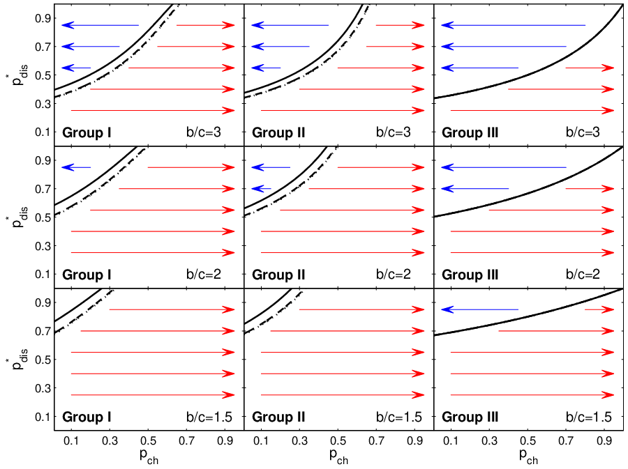
We have studied the stability of the leading eight strategies against the invasion of cheaters. We divided the leading eight strategies in Groups I, II and III as a function of its different behavior (as it was done in [16]). Figure 2 represents the limiting $p^{*}_{\text{dis}}$ below (above) which mutants who cheat with a higher (lower) probability than residents can invade. In Appendix B we calculate analytically the shape of this curve in the limit $\epsilon_{A}\to 0$ . Figure 2 shows that below the curve $p^{*}_{\text{dis}}(p_{\text{ch}})$ cheating increases without bound through subsequents invasions until the whole population is dominated by defectors. In other words, if cheating occurs and the probability of being discovered is not high enough, none of the leading eight strategies survives. In particular, if $p_{\text{dis}}<c/b$ full defection is the unavoidable fate of the population. Thus, if only small mutations are allowed in a honest population, we find the Hamilton-like rule $bp_{\text{dis}}>c$ for the survival of cooperation [28].

Increasing $\epsilon_{A}$ makes it even easier for cheaters to invade, with the exception of the strategies belonging to Group III, which seem to be insensitive to the effect of errors in action.

V Discussion

We have carried out a systematic study of the stability of all possible third-order indirect reciprocity strategies. We extended the work of Ohtsuki and Iwasa [16] confronting all the strategies against the others regardless of whether they have the same moral assessments or not. The main difference with their model is that in ours individuals directly witness all actions. Allowing individuals in the same population to have different moral assessments and action rules makes indirect observation models computationally unfeasible (we must store everybody’s opinion of everybody else at every time step). For the same reason, errors in judgments cannot be accounted for in direct observation models. Thus we only consider errors in performing the actions. The only exception to this assumption is the need to introduce errors in judgement to calculate, in some special cases, the stationary fractions of good and bad individuals in homogeneous populations. But this is just a technical issue that allows us to resolve a degeneracy of solutions, and there is no inconsistency because the results do not depend on the value of this error.

The strategies which are stable against invasions by other strategies sharing the same moral assessment turn out to be also stable against invasions by any other strategy. This means that if a strategy can resist the invasion of all the other strategies that share its same moral assessment, it can resits any invasion whatsoever.

We have checked that the higher the benefit-to-cost ratio and the lower the action errors the higher the number of stable strategies obtained. One possible interpretation of the errors in action is lack of resources. Under this interpretation our results show that scarcity of resources favors invasions. On the other hand, we have checked that populations whose members receive more benefit for a given cost are more resistant to invasions.

As pointed out in Ref. [16], there is a symmetry between the moral assessments of the strategies. Good and bad are just labels with no proper meaning—in contrast to actions, that have a direct influence in the payoffs. In order to break that symmetry and provide a meaning to those labels we have introduced the concept of coherence. Coherence links moral assessments with action rules. We have shown that stable strategies appear in pairs due to the above mentioned symmetry, but coherence values are complementary. This allows us to choose only one of the strategies (the most coherent) within each pair for later analysis and interpretation.

The stable strategies we obtain include the Leading Eight found by Ohtsuki and Iwasa [16]. These are also the most efficient ones (those with highest payoffs). Both the Leading Eight as well as the remaining stable strategies that we have obtained share some features, and except for the two least efficient strategies (with $\widetilde{W}_{H}=0.25$ ), all of them obtain high average payoffs ( $\widetilde{W}_{H}>0.8$ ). They identify defectors ( $m_{GG}(D)=m_{BG}(D)=B$ ) and, except the two least efficient strategies, maintain cooperation ( $a_{GG}=C$ and $m_{GG}(C)=G$ ). All of them punish defectors ( $a_{GB}=D$ ), although three of the stable strategies (with $\widetilde{W}_{H}\sim 0.9$ ) do not judge this as a good behavior. Finally the most efficient stable strategies ( $\widetilde{W}_{H}>0.9$ ) forgive bad individuals who help good players ( $m_{BG}(C)=G$ and $a_{BG}=C$ ). The more of these features the strategies follow the higher their payoff. For instance, the three strategies with $\widetilde{W}_{H}\sim 0.9$ turn good punishers into bad individuals and they can only restore their reputation by helping good individuals. And in the case of strategies with $\widetilde{W}_{H}<0.9$ , bad individuals cannot increase their reputation by helping good players, but only by interacting with other bad individuals.

We have also found that all these strategies may become unstable if cheaters arise. If the probability of witnessing a cheat is not high enough, cheaters can take over an honest population. Upon increasing the cheating probability $p_{\text{dis}}>c/b$ the population eventually turns into pure defectors. Interestingly, the condition for a population to resist this effect is of the Hamilton type, namely, $bp_{\text{dis}}>c$ , where $b$ is the benefit and $c$ the cost. Errors in action make this condition even more restrictive for the stability of a honest population.

Cheating is always a danger for cooperation based on indirect reciprocity. Even in societies where this mechanism is of utmost importance cheating always threats honest behavior. For instance, the (now extinct) Patagonian tribes of the Yámana are among the reported societies more strongly based on indirect reciprocity [29]. Sharing food even with nonrelatives appeared to be the default behavior. Not sticking to it brought a bad reputation and severe social pubishment (e.g., not participating in further food sharing). Yet, cheating among the Yámana was reported to occur when chances were low to be discovered (for instance, because the prey obtained was easy to hide; see Ref. [29], p. 197).

One of the problems that emerges from considering different moral assessments is the possibility that the fractions of good and bad individuals may depend on the initial setup. We sort out this issue by choosing realistic initial conditions for the differential equations describing the evolution of these fractions. Essentially, we assume that mutations do not change the previous judgments that individuals had on each other. This notwithstanding, we have analyzed other initial conditions in which not all individuals have the same opinion. A typical setup where this might happen is when a rumor is spread over a fraction of the population. We have checked that, although misjudgement can survive or even spread over a larger fraction of the population, it eventually disappears because mutants with a wrong judgement get less payoff than residents who use one of the stable strategies.

Admittedly, in order to carry out such a systematic analysis as we have performed here, we have had to sacrifice some realism in the model. On the one hand, we have considered that reputation can only have two states: good and bad. This binary reputation have been used in several preceding studies [16, 23] and implies that only the actions that happen in the last round are taken into account to assign reputation. However, Tanabe et al. [30] have studied a model with trinary reputations and showed that some strategies (like the so-called image scoring) can be stable in a trinary-reputation model but not in a binary-reputation one. On the other hand, we have considered that every player has complete information of every single interaction in the population (except when we introduced cheating). This is too strong an assumption and some studies discuss the effect of a limited access to the information (see [31] and the references therein).

Acknowledgments

We are indebted to Prof. Karl Sigmund for his hospitality in hosting LAMV and his valuable insights. We also thank Ivan Briz for sharing his archaeological knowledge with us. This work has been supported by Ministerio de Ciencia e Innovación (Spain) through grants MOSAICO and PRODIEVO, by European Research Area Complexity-Net through grant RESINEE, and by Comunidad de Madrid (Spain) through grant MODELICO-CM. LAMV was supported by a postdoctoral fellowship from Alianza 4 Universidades.

Appendix A

The two sets of Eqs. (8) and (9) can be simplified in the steady state $dx/dt=0$ . Thus, summing over the reputation $\Lambda_{2}$ in Eqs. (8) we obtain

x_{1}^{G*}=\sum_{\Lambda_{2}}x_{1}^{G\Lambda_{2}}=x_{1H}.

(16)

Therefore we can reduce Eqs. (8) to just two equations in two unknowns (e.g., $x_{1}^{GG}$ and $x_{1}^{BB}$ ) by setting

\begin{split}&x_{1}^{GB}=x_{1}^{G*}-x_{1}^{GG},\\ &x_{1}^{BG}=1-x_{1}^{G*}-x_{1}^{BB}.\end{split}

(17)

The two remaining equations from (8) have to be solved numerically using the initial conditions discussed in Sec. III.2.

On the other hand, the set of Eqs. (9) is decoupled from the set (8), and so they can be solved analytically after solving the latter. This is easier if $x_{2}^{*G}$ is calculated first,

\begin{split}x_{2}^{*G}=&\left[x_{1}^{*G}P_{2,01}+(1-x_{1}^{*G})P_{2,00}\right]\\ &\times\left[1+x_{1}^{*G}(P_{2,01}-P_{2,11})\right.\\ &\left.+(1-x_{1}^{*G})(P_{2,00}-P_{2,10})\right]^{-1}.\end{split}

(18)

Hence Eq. (9) reduces to a linear system of two equations in the two unknowns $x_{2}^{GG}$ , $x_{2}^{BB}$ .

There are scenarios where the solution of $x_{2}^{\Lambda_{1}\Lambda_{2}}$ turns out to be degenerated. In these situations the set of Eqs. (9) need to be integrated along with the set of Eqs. (8).

Appendix B

Consider a resident population whose individuals play one of the leading eight strategies with probability $1-p_{\text{\text{ch}},1}$ but defect otherwise. Consider mutants who do the same, but with a probability $1-p_{\text{ch},2}$ . For simplicity let us assume the limiting case $\epsilon_{A}\to 0$ . Applying adaptive dynamics [32], the curve separating the regions where the mutant can or cannot invade the population is given by

\left.\frac{dW(p_{\text{\text{ch}},2},p_{\text{ch},1})}{dp_{\text{ch},2}}\right|_{p_{\text{ch},2}=p_{\text{ch},1}}=0,

(19)

where the payoff $W(p_{\text{\text{ch}},2},p_{\text{ch},1})$ is equivalent to $W(2|1)$ . According to Eq. (12),

\frac{dW(p_{\text{\text{ch}},2},p_{\text{ch},1})}{dp_{\text{ch},2}}=b\frac{d\theta^{ch}_{1,2}}{dp_{\text{ch},2}}-c\frac{d\theta^{ch}_{2,1}}{dp_{\text{ch},2}}.

(20)

To go further we need to separate the strategies of the three groups.

B.1 Group I strategies

Using Eqs. (15) for the leading eight strategies, the probabilities of cooperation $\theta^{\text{ch}}_{i,j}$ are

\begin{split}\theta^{\text{ch}}_{1,2}=&(1-p_{\text{\text{ch}},1})\left[x_{2}^{\text{ch}}+(1-x_{1,H}^{\text{ch}})(1-x_{2}^{\text{ch}})\right],\\ \theta^{\text{ch}}_{2,1}=&(1-p_{\text{\text{ch}},2})\left[x_{1,H}^{\text{ch}}+(1-x_{1,H}^{\text{ch}})(1-x_{2}^{\text{ch}})\right].\end{split}

(21)

Thus

\begin{split}\dfrac{d\theta^{\text{ch}}_{1,2}}{dp_{\text{ch},2}}=&(1-p_{\text{\text{ch}},1})\,x_{1,H}^{ch}\,\dfrac{dx_{2}^{ch}}{dp_{\text{ch},2}},\\ \dfrac{d\theta^{\text{ch}}_{2,1}}{dp_{\text{ch},2}}=&(1-x_{1,H}^{\text{ch}})\left[x_{2}^{ch}-(1-p_{\text{ch},2})\,\dfrac{dx_{2}^{ch}}{dp_{\text{ch},2}}\right]-1.\end{split}

(22)

The fractions $x_{1,H}^{\text{ch}}$ and $x_{2}^{ch}$ are obtained from Eqs. (4) and (18). To that purpose we need to substitute

P_{i,11}^{\text{ch}}=P_{i,01}^{\text{ch}}=1-p_{\text{dis}}p_{\text{ch},i},\qquad P_{i,10}^{\text{ch}}=1

(23)

and

P_{i,00}^{\text{ch}}=1-p_{\text{dis}}p_{\text{ch},i}.

(24)

Thus $x_{1,H}^{\text{ch}}$ is the solution of

p_{\text{dis}}p_{\text{ch},1}(x_{1,H}^{\text{ch}})^{2}=(1-p_{\text{dis}}p_{\text{ch},1})(1-x_{1,H}^{\text{ch}}),

(25)

and once it is obtained,

\begin{split}&x_{2}^{\text{ch}}=\frac{1-p_{\text{dis}}p_{\text{ch},2}}{1-(1-x_{1,H}^{\text{ch}})p_{\text{dis}}p_{\text{ch},2}},\\ &\dfrac{dx_{2}^{\text{ch}}}{dp_{\text{ch},2}}=-\frac{p_{\text{dis}}x_{1,H}^{\text{ch}}}{[1-(1-x_{1,H}^{\text{ch}})p_{\text{dis}}p_{\text{ch},2}]^{2}}.\end{split}

(26)

Substituting into (22) and setting $p_{\text{ch},2}=p_{\text{ch},1}\equiv p_{\text{ch}}$ yields

\begin{split}\dfrac{d\theta^{\text{ch}}_{1,2}}{dp_{\text{ch}}}=&-\frac{(1-p_{\text{ch},1})p_{\text{dis}}(x_{1,H}^{\text{ch}})^{2}}{[1-p_{\text{dis}}p_{\text{ch}}(1-x_{1,H}^{\text{ch}})]^{2}},\\ \dfrac{d\theta^{\text{ch}}_{2,1}}{dp_{\text{ch},2}}=&\frac{x_{1,H}^{\text{ch}}[p_{\text{dis}}(1-x_{1,H}^{\text{ch}})-1]}{[1-p_{\text{dis}}p_{\text{ch}}(1-x_{1,H}^{\text{ch}})]^{2}}.\end{split}

(27)

Therefore $p_{\text{dis}}^{*}$ is the solution of the system

\begin{split}&p_{\text{dis}}^{*}[b(1-p_{\text{ch}})x^{*}+c(1-x^{*})]=c,\\ &p_{\text{dis}}^{*}p_{\text{ch}}(x^{*})^{2}=(1-p_{\text{dis}}^{*}p_{\text{ch}})(1-x^{*}).\end{split}

(28)

B.2 Group II strategies

For the strategies of this group

\theta^{\text{ch}}_{1,2}=(1-p_{\text{\text{ch}},1})\,x_{2}^{\text{ch}},\qquad\theta^{\text{ch}}_{2,1}=(1-p_{\text{\text{ch}},2})\,x_{1,H}^{\text{ch}},

(29)

hence their derivatives are

\dfrac{d\theta^{\text{ch}}_{1,2}}{dp_{\text{ch},2}}=(1-p_{\text{\text{ch}},1})\,\dfrac{dx_{2}^{ch}}{dp_{\text{ch},2}},\qquad\dfrac{d\theta^{\text{ch}}_{2,1}}{dp_{\text{ch},2}}=-x_{1}^{\text{ch}}.

(30)

Probabilities $P_{i,\alpha\beta}^{\text{ch}}$ are now given by (23) as well as $P_{i,00}^{\text{ch}}=1$ . Thus, after Eqs. (4) and (18),

x_{1,H}^{\text{ch}}=\frac{1}{1+p_{\text{dis}}p_{\text{\text{ch}},1}},\qquad x_{2}^{\text{ch}}=1-x_{1,H}^{\text{ch}}p_{\text{dis}}p_{\text{\text{ch}},2}.

(31)

Substituting into (30) and setting $p_{\text{ch},2}=p_{\text{ch},1}\equiv p_{\text{ch}}$ yields

\begin{split}\dfrac{d\theta^{\text{ch}}_{1,2}}{dp_{\text{ch},2}}=&-\frac{(1-p_{\text{ch}})p_{\text{dis}}}{1+p_{\text{dis}}p_{\text{ch}}},\\ \dfrac{d\theta^{\text{ch}}_{2,1}}{dp_{\text{ch,2}}}=&-\frac{1}{1+p_{\text{dis}}p_{\text{ch}}},\end{split}

(32)

and therefore

p_{\text{dis}}^{*}=\dfrac{c}{b\,(1-p_{\text{ch}})}.

(33)

B.3 Group III strategies

For the strategies of this group the probabilities of cooperation and their derivatives are also given by Eqs. (29) and (30), and the probabilities $P_{i,\alpha\beta}^{\text{ch}}$ by (23) as well as $P_{i,00}^{\text{ch}}=0$ . Thus, after Eqs. (4) and (18),

x_{1,H}^{\text{ch}}=1-p_{\text{dis}}p_{\text{\text{ch}},1},\qquad x_{2}^{\text{ch}}=1-p_{\text{dis}}p_{\text{\text{ch}},2}.

(34)

Substituting into (30) and setting $p_{\text{ch},2}=p_{\text{ch},1}\equiv p_{\text{ch}}$ yields

\begin{split}\dfrac{d\theta^{\text{ch}}_{1,2}}{dp_{\text{ch},2}}=&-(1-p_{\text{ch}})p_{\text{dis}},\\ \dfrac{d\theta^{\text{ch}}_{2,1}}{dp_{\text{ch,2}}}=&-(1-p_{\text{dis}}p_{\text{ch}}),\end{split}

(35)

and therefore

p_{\text{dis}}^{*}=\dfrac{c}{c\,p_{\text{ch}}+b\,(1-p_{\text{ch}})}.

(36)

References

[1] E. Fehr and U. Fischbacher, Nature 425, 785 (2003).
[2] R. L. Trivers, Q. Rev. Biol. 46, 35 (1971).
[3] R. Sugden, The economics of rights, co-operation and welfare (Basil Blackwell, Oxford, 1986).
[4] R. D. Alexander, The Biology of Moral Systems (New York: Aldine de Gruyter, 1987).
[5] M. Dufwenberg, U. Gneezy, W. Güth, and E. van Damme4, Homo Oeconomicus 18, 19 (2001).
[6] M. Milinski, D. Semmann, and H. J. Krambeck, Nature 415, 424 (2002).
[7] K. Panchanathan and R. Boyd, Nature 432, 499 (2004).
[8] D. Semmann, H.-J. Krambeck, and M. Milinski, J. Behav. Ecol. Sociobiol. 56, 248 (2004).
[9] S. Suzuki and E. Akiyama, J. Theor. Biol. 245, 539 (2007).
[10] R. Bshary and A. S. Gutter, Nature 441, 975 (2006).
[11] G. E. Bolton, E. Katok, and A. Ockenfels, Manage. Sci. 50, 1587 (2005).
[12] C. Keser, IBM Syst. J. 43, 498 (2002).
[13] R. Boyd and P. J. Richerson, Social Networks 11, 213 (1989).
[14] M. A. Nowak and S. Roch, Proc. R. Soc. B 274, 605 (2007).
[15] M. A. Nowak and K. Sigmund, Nature 393, 573 (1998).
[16] H. Ohtsuki and Y. Iwasa, J. Theor. Biol. 231, 107 (2004).
[17] H. Brandt and K. Sigmund, J. Theor. Biol. 231, 475 (2004).
[18] M. A. Nowak and K. Sigmund, Nature 437, 1291 (2005).
[19] O. Leimar and P. Hammerstein, Proc. R. Soc. Lond. B 268, 745 (2001).
[20] J. M. Pacheco, A. Traulsen, and M. A. Nowak, Phys. Rev. Lett. 97, 258103 (2006).
[21] H. Ohtsuki and Y. Iwasa, J. Theor. Biol. 244, 518 (2007).
[22] H. Ohtsuki and Y. Iwasa, J. Theor. Biol. 239, 435 (2006).
[23] S. Uchida and K. Sigmund, J. Theor. Biol. 263, 13 (2010).
[24] L. A. Martinez-Vaquero, J. A. Cuesta, and A. Sánchez, PLoS ONE 7, e35135 (2012).
[25] K. Panchanathan and R. Boyd, J. Theor. Biol. 224, 115 (2003).
[26] M. A. Fishman, J. Theor. Biol. 225, 285 (2003).
[27] A. Lotem, M. A. Fishman, and L. Stone, Nature 400, 226 (1999).
[28] W. D. Hamilton, J. Theor. Biol. 7, 1 (1964).
[29] L. A. Orquera and E. L. Piana, La vida material y social de los Yámana (Eudeba-IFIC, Buenos Aires, 1999).
[30] S. Tanabe, H. Suzuki, and N. Masuda, arXiv:1205.3547v2 (2012).
[31] M. Nakamura and N. Masuda, PLoS Comput. Biol. 7, e1002113 (2011).
[32] J. Hofbauer and K. Sigmund, Evolutionary Games and Population Dynamics (Cambridge University Press, Cambridge, 1998).