Initial state dependence of the quench dynamics in integrable quantum systems.
III.
Chaotic states
Abstract
We study sudden quantum quenches in which the initial states are selected to be either eigenstates of an integrable Hamiltonian that is nonmappable to a noninteracting one or a nonintegrable Hamiltonian, while the Hamiltonian after the quench is always integrable and mappable to a noninteracting one. By studying weighted energy densities and entropies, we show that quenches starting from nonintegrable (chaotic) eigenstates lead to an “ergodic” sampling of the eigenstates of the final Hamiltonian, while those starting from the integrable eigenstates do not (or at least it is not apparent for the system sizes accessible to us). This goes in parallel with the fact that the distribution of conserved quantities in the initial states is thermal in the nonintegrable cases and nonthermal in the integrable ones, and means that, in general, thermalization occurs in integrable systems when the quench starts form an eigenstate of a nonintegrable Hamiltonian (away from the edges of the spectrum), while it fails (or requires larger system sizes than those studied here to become apparent) for quenches starting at integrable points. We test those conclusions by studying the momentum distribution function of hard-core bosons after a quench.
pacs
02.30.Ik,05.30.-d,03.75.Kk,05.30.JpI Introduction
The experimental realization of ultracold quantum gases in (quasi-)one-dimensional (1D) geometries has stimulated much theoretical research on 1D systems [1]. In equilibrium, they are particularly interesting because of the enhanced role played by quantum fluctuations. In addition, when taken out of equilibrium, they may exhibit unique behavior such as lack of thermalization [2, 3]. We note that ultracold gases are well isolated by the ultra high vacuum in which they are confined, i.e., their dynamics is to a very good approximation unitary [4]. Hence, by lack of thermalization we mean the fact that, after perturbing the system and letting it evolve, experimental observables relax to time-independent values that are not described by conventional statistical ensembles. This effect has been attributed to the proximity to integrable points [5, 6, 7, 8], and has motivated an extensive exploration of the dynamics of integrable systems [8, 9, 10, 11, 12, 13, 14, 15, 16, 17, 18, 19, 20, 21, 22, 23, 24, 25, 26, 27].
The most common dynamics studied in this context are the ones that occur after so-called sudden quenches. In a sudden quench, the initial state is selected to be an eigenstate of an initial Hamiltonian (). Then, at time , some parameter(s) of is(are) changed instantaneously , and the time evolution is followed under the final (time-independent) Hamiltonian ():
| (1) |
where are the overlaps of the initial state with the eigenstates of the final Hamiltonian.
Within this protocol, the time evolution of the expectation value of an observable , , can be written as
| (2) |
where . If the observable relaxes to a time-independent value (up to fluctuations that vanish, and revival times that diverge, in the thermodynamic limit), that value can be computed (up to corrections that vanish in the thermodynamic limit) by taking the infinite-time average of Eq. (2):
| (3) |
where we have assumed that there are no degeneracies, or that they can be neglected. The infinite-time average can be thought of as the prediction of an ensemble, the “diagonal ensemble” [8], where the density matrix is diagonal in the basis of eigenstates of the final Hamiltonian, i.e., .
Several theoretical studies have shown that in integrable systems, and for observables of interest in current experiments and models, is different from the predictions of conventional statistical mechanics ensembles [8, 9, 10, 18, 25, 26]. Among the (few-body) observables that have been studied are the density and momentum distribution function of hard-core bosons [8, 9, 10], the double occupancy of fermions [18], and spin-spin correlations in spin chains [25, 26]. If one wants to go beyond conventional statistical mechanics ensembles to take into account that nontrivial conserved quantities (whose number scales polynomially with system size) are present in integrable systems, and maximizes the entropy under those constraints [28, 29], then a generalized Gibbs ensemble (GGE) is obtained [8]. Remarkably, the GGE has been shown to provide the correct description for the previously mentioned observables (and others) after relaxation following a sudden quench [8, 9, 10, 13, 14, 15, 16, 17, 18, 24, 25, 26]. The (grand-canonical) density matrix for the GGE can be written as [8]
| (4) |
where is the partition function, are conserved quantities, and are their corresponding Lagrange multipliers. The latter are computed using that .
The lack of thermalization of few-body observables of interest in integrable systems has been attributed to the failure of the eigenstate thermalization hypothesis [5, 6, 7, 10, 30, 31]. That is to say that, within a microcanonical window, the matrix elements in an integrable system fluctuate over a finite range of values. Hence, the outcome of the quench dynamics depends on which eigenstates of the final Hamiltonian have a finite overlap with the initial state. If the initial state samples the eigenstates within the microcanonical window in an un-bias way, i.e., “ergodically,” then for that initial state the integrable system will thermalize. This does not happen for most quenches between integrable systems studied in the literature [8, 9, 10, 13, 14, 15, 17, 18, 24, 25, 26]. However, it has been shown to occur for special initial states [11] with particular entanglement properties [16], as well as for initial thermal states at infinite temperature [12]. In the latter work, finite temperatures were shown to lead to a bias sampling of the final eigenstates of the Hamiltonian after a quench.
In this work, we study what happens in quenches from initial states that are eigenstates of an integrable Hamiltonian that is nonmappable to a noninteracting one, while the final Hamiltonian is integrable and mappable to a noninteracting one. This is of interest as most studies in the literature have focused on quenches where both the initial and final Hamiltonians are mappable to noninteracting ones. We also study the case in which the initial state is an eigenstate of a nonintegrable Hamiltonian and the final Hamiltonian is integrable. As argued in Ref. [32], initial states that are eigenstates of nonintegrable Hamiltonians (away from the edges of the spectrum [33, 34]) can lead to thermalization even though the final Hamiltonian is integrable. This can be understood as the two-body interactions that break integrability in models of current interest lead to quantum chaos even in the absence of randomness [33, 34, 35, 36], similar to what happens in systems with two-body random interactions [37, 38, 39, 40]. As a result, the eigenstates of nonintegrable Hamiltonians become random superpositions of eigenstates of the integrable ones to which the quench is performed, i.e., they provide the unbiased sampling required for thermalization after a quench to integrability. We do not find indications that this happens in quenches between the integrable systems studied here.
The exposition is organized as follows. In Sec. II, we introduce the model Hamiltonian and describe the quenches to be studied. The observables and ensembles of interest are introduced in Sec. III. The remainder sections are devoted to the discussion of the results for: (i) overlaps between initial states and eigenstates of the final Hamiltonians (Sec. IV), (ii) entropies (Sec. V), (iii) conserved quantities (Sec. VI), and (iv) momentum distribution functions (Sec. VII). A summary of the results is presented in Sec. VIII.
II Model Hamiltonian and Quenches
We focus our study on 1D lattice hard-core bosons in a box (a system with open boundary conditions) with nearest-neighbor (NN) hopping and interaction , and next-nearest-neighbor (NNN) hopping and interaction . The Hamiltonian reads
| (5) |
where is the hard-core boson creation (annihilation) operator, the number operator, and is the lattice size. In addition to the usual commutation relations , and satisfy the constraints , which preclude multiple occupancy of the lattice sites. In what follows, the NN hopping parameter sets the energy scale (), we take (where is the Boltzman constant), and the number of particles is selected to be .
For , Hamiltonian (5) is integrable (it can be mapped onto the spin-1/2 chain) [1]. For , it is nonmappable to a noninteracting model. However, if , one can exactly solve Hamiltonian (5) by first mapping it onto the spin-1/2 chain through the Holstein-Primakoff transformation [41] and then onto noninteracting fermions by means of the Jordan-Wigner transformation [42], i.e., it is mappable to a noninteracting model. Hence, the many-body eigenstates of the fermionic counterpart are Slater determinants that can obtained from the single-particle Hamiltonian without the need of diagonalizing the many-body one. Properties of Slater determinants allow one to calculate off-diagonal correlations of hard-core bosons in polynomial time both in the many-body eigenstates of the Hamiltonian [43, 44, 45] and in the grand-canonical ensemble [46]. The presence of nonzero NNN terms break the integrability of the model and drive the system to a chaotic regime [33, 34, 35, 36].
Here, we consider two types of quenches. Quench type I is within integrable models, i.e, we keep at all times, and select the initial state to be an eigenstate of Hamiltonian (5) with , while the evolution is studied under Hamiltonian (5) with . Quench type II is from a nonintegrable model to an integrable one: Namely, the initial state is selected to be an eigenstate of Hamiltonian (5) with while the dynamics is studied under Hamiltonian (5) with . In quench type II, we keep at all times. Note that the final Hamiltonian in both types of quenches is the same. One can fully diagonalize it for large systems by mapping it onto noninteracting fermions as mentioned before. Since and are only present in the initial Hamiltonian, in what follows we drop the subindex “” from and .
In order to compare results of quenches from eigenstates of different initial Hamiltonians, we select the initial states such that after the quench the systems have an energy
| (6) |
which always corresponds to that of the canonical ensemble (CE) at a fixed temperature (the temperature is taken to be throughout this work). This means that , where is the CE density matrix, and is the partition function. The initial states, which are eigenstates of the - and -- models, i.e., none of which is mappable to a free model, are computed by means of the FILTLAN package that utilizes a polynomial filtered Lanczos procedure [47]. Since open boundary conditions are imposed, the only remaining symmetry at 1/3 filling, and for , is parity. Here, we restrict our analyses to the even parity sector, the dimension of which is about 1/2 of the entire Hilbert space. The largest systems we study have , whose total Hilbert space dimension is . The even parity subspace for those systems has dimension . This is more than ten times larger than the largest Hamiltonian sector diagonalized in previous full exact diagonalization studies of similar systems [6, 7, 33, 34, 35, 36]. In this work, the combination of utilizing the Lanczos algorithm for computing the initial state, and full exact diagonalization via the Bose-Fermi mapping for the final Hamiltonian, is what allows us to perform a complete analysis for larger Hilbert spaces.
III Ensembles and Observables
Given the fact that the initial states () are pure states, and that the dynamics is unitary, the von Neumann entropy is zero at all times. In order to characterize our isolated systems, we make use of the diagonal entropy . It is defined as the von Neumann entropy of the diagonal ensemble [48],
| (7) |
and satisfies all thermodynamic properties expected of an entropy [48]. has been recently shown to be consistent with the entropy of thermal ensembles for generic (nonintegrable) systems after relaxation [49].
Similar to the studies in Refs. [11, 12], we compare the DE with the entropy predicted by the CE, the grand-canonical ensemble (GE), and the GGE. Namely, we also compute
| (8) | |||||
| (9) | |||||
| (10) |
where was defined in Eq. (6), and , , , and were also defined before. In Eq. (9), the chemical potential and the temperature are computed such that and , where is the GE density matrix, is the partition function, and is the total number of particle operator. We note that while the differences between all those entropies are expected to be finite for any finite system, our goal here is to understand how those differences behave with increasing system size.
As mentioned before, all our quenches share the same final Hamiltonian (), which is integrable. The conserved quantities for the GGE in that model are taken to be the occupation number operators of the single particle eigenstates of the fermionic Hamiltonian to which hard-core bosons can be mapped. From this selection, it follows straightforwardly that the corresponding Lagrange multipliers can be computed as [8]. Note that, by construction, the GGE has the same distribution of conserved quantities as the diagonal ensemble. We also calculate the distribution of conserved quantities predicted by the GE, namely, .
In addition, we study the momentum distribution function of hard-core bosons in the DE (), the GE (), and the GGE (). is the diagonal part of the Fourier transform of the one-particle density matrix operator ,
| (11) |
and it was previously studied in systems out of equilibrium with the same in Refs. [8, 9, 10].
IV overlaps
As mentioned before, in integrable systems, the lack of eigenstate thermalization implies that the distribution of overlaps of the initial state with the eigenstates of final Hamiltonian plays a very important role in determining the expectation value of observables after relaxation [Eq. (2)]. Therefore, we first study the values of as a function of in quenches type I and type II and compare them to the weights of the eigenstates of the final Hamiltonian in the CE, .

In Fig. 1, we show density plots of the coarse-grained values of for different type I quenches [Figs. 1(a)–1c)] and type II [Figs. 1(e)–1(h)]. The corresponding results for the canonical weights () are presented in Figs. 1(d) and 1(h). One can see in Fig. 1 that, for all values of in quench type I and in quench type II, the distribution of weights in the DE is qualitatively distinct from that in the CE, which shows a simple exponential decay. In the diagonal ensemble, the weights between eigenstates that are close in energy fluctuate wildly (note the logarithmic scale in the axes), and a maximum in the values of [particularly clear in panels (a), (b), (e) and (f)] can be seen around the energy of the initial state after the quench . Hence, in contrast to the canonical ensemble, eigenstates of whose energies are close to usually have the largest weights. This was also seen in Ref. [50].
Another feature that is apparent in Fig. 1 is that while the weights decrease rapidly as one moves away from , the number of states with those weights increases dramatically for due to the increase of the density of states. For this reason, the appropriate quantity to quantify how different regions of the spectrum contribute to the observables in the diagonal ensemble (and in the CE) is the weighted energy density function,
| (12) |
where is for the DE and for the CE. The summation is limited to the states in a small energy window , the width of which () is selected to be the same as for the coarse graining in Fig. 1. We have checked that our results are robust for the selected values of .

The weighted energy density functions for the quenches studied in Fig. 1 are shown in Fig. 2. There one can see that in all cases, except for the strongest quenches type II, in the CE is much broader than that in the DE. For comparison, we have also plotted the results for the energy shells, which are Gaussians with the same mean energy and energy width as the diagonal ensemble. The energy shell has the maximal number of eigenstates of the final Hamiltonian that is accessible to the particular initial state selected. In quenches type I [Figs. 2(a)-2(c)], even for the largest , in the diagonal ensemble remains narrower than the energy shell. This is an indication of the lack of “ergodicity” of the initial states associated with quench type I. On the contrary, in quenches type II [Figs. 2(d)-2(f)], the width of in the diagonal ensemble approaches that of the energy shell with increasing . For the strongest quench considered, [51], in the DE and the CE become very close to each other as well as to the energy shell [Fig. 2(f)]. The latter shows that initial states that are eigenstates of nonintegrable Hamiltonians sufficiently distant from an integrable point fill the energy shell ergodically after a quench to integrability.
To better characterize as one goes from the weakest to the strongest quenches, we have fitted it to two different functions: (i) a Breit-Wigner function,
| (13) |
and (ii) a Gaussian,
| (14) |
where the mean energy and half-width of the Breit-Wigner function, as well as the mean energy and half-width of the Gaussian, are taken as fitting parameters.
Figures 2(a)-2(c) show that, as the strength of the interaction increases in quenches type I, the weighted energy densities in the DE are better described by Breit-Wigner functions. In quenches type II [Figs. 2(d)-2(f)], on the other hand, weighted energy densities are described by Breit-Wigner functions for weak quenches and transition to Gaussians as the strength of the quench increases. The fact that in the latter quenches approach Gaussians (and ultimately the energy shell) hints the possibility of observing thermalization in those cases. This is consistent with the results in Refs. [35, 36], which considered a different set of quench protocols and were averaged over different initial states. Note that, in our results, no average has been introduced.
Using the Breit-Wigner function to fit the weighted energy densities for the quenches type I, as well as the weakest quench type II, is motivated by analytic results obtained in the random two-body interaction model [37, 38, 39, 40], and by recent numerical results for models similar to those considered here [35, 36]. In Refs. [35, 36], the weighted energy densities (which were called strength functions) were computed for the reverse quenches to those considered here, namely, starting from a state that is an eigenstate of an integrable Hamiltonian (in one case, our ) and projecting that state onto the eigenstates of the - and -- Hamiltonians (our ), i.e., . In our notation, the weighted energy densities from those works can be written as
| (15) |
where the sum runs over states in the spectrum of within a small window of energy . Correspondingly, the energy shell associated with is now a Gaussian centered at whose width is .

For chaotic systems, it was shown in Refs. [37, 38, 39, 40, 35, 36], that as the interaction strength increases, and the average strength of the coupling between unperturbed eigenstates becomes of the order of the average unperturbed level spacing, transitions from a Breit-Wigner function to a Gaussian. This transition also seen numerically in integrable systems [35, 36] through an analysis of states whose energy was in the center of the spectrum, i.e., whose . In order to make contact with the results in Refs. [35, 36], we compute for our quenches and in the regions of the spectrum relevant to out work. Note that since full exact diagonalization is required to obtain all eigenstates , the largest systems considered here in the calculations of have and . Finite size effects are strong for those lattice sizes, so we average the results for over the nine even parity states that are closest in energy to
In Fig. 3, we show results for for the same Hamiltonian parameters for which we previously studied the weighted energy densities. Comparing Fig. 3 and Fig. 2, one can see that the results for and are qualitatively similar. For both types of quenches, becomes broader with increasing (integrable) and (nonintegrable). However, when is integrable, remains better described by Breit-Wigner functions, while a transition from Breit-Wigner to Gaussian behavior, as well as a filling of the energy shell [better seen in Fig. 3(f) than in Fig. 2(f)], is only observed for a nonintegrable .
Our results for integrable systems are in contrast to those reported in Refs. [35, 36], where a transition from Breit-Wigner to Gaussian was also observed for an interaction quench within integrable systems. This can be attributed to the combination of two effects. One is the fact that the states selected here are far from the middle of the spectrum, as was the case in Ref. [35, 36]. Within the entire spectrum, the mean level spacing in the middle is the minimal one, i.e., the same perturbation may couple more states in that region than away from it. If the average level spacing is the only reason for the difference, then a transition should be seen in our case as one increases the system size even further. This is a possibility that cannot be excluded within the present study.
However, there may be another reason which would make the differences remain in the thermodynamic limit. The result of averaging over eigenstates in the middle of the spectrum [35, 36] leads to an ensemble at infinite temperature. In that ensemble, the distribution of the quantities that are conserved after the quench could be featureless. This would result in an un-bias sampling of the eigenstates of the Hamiltonian after the quench, which may not occur for quenches starting at a finite temperature even if they are strong quenches. We have found this to be the case in quenches in systems with in which one starts from a thermal state [12]. Only the initial state at infinite temperature was found to ergodically sample the eigenstates after the quench, and a finite size scaling analysis showed that this does not change with increasing system size. We will come back to this point in Sec. VI, where the conserved quantities are studied for all quenches considered here.
V entropies

The fact that the weighted energy density appears to be Gaussian after a quench to integrability does not automatically guaranty that thermalization will occur, as it does not mean that an un-bias sampling has been performed (unless the energy shell is filled). One needs to keep in mind that a coarse-graining is involved when calculating , where [see Eq. (12)] is much larger than the average level spacing. For example, in Ref. [12], we showed that quenches between integrable systems, which started from thermal states, led to Gaussian like weighted energy distributions that are not thermal and do not become thermal with increasing system size. The exception was the initial infinite temperature state, which does lead to a thermal distribution after a quench (but at infinite temperature). A qualitatively similar behavior was seen for quenches starting from special pure states that are ground states of an integrable Hamiltonian [11].
In order to quantify how the weights evolve in the DE as the system size increases, and how they compare to the weights in the GGE, CE, and GE, we have computed the entropies of the corresponding ensembles for all the quenches studied before. In Fig. 4, we show all those entropies, per site, as a function of for quenches type I [Figs. 4(a)–4(d)] and of for quenches type II [Figs. 4(e)–4(h)], for four system sizes. Since, in all cases, we consider a fixed effective temperature after the quench, the values of in the CE and the GE are (almost) independent of the quench parameters.
The first feature that is apparent in Fig. 4 is that, in both types of quenches, the entropy in the DE and the GGE are very small for weak quenches and increase as system size increases. The GGE entropy follows (but is always above, as expected from its grand-canonical nature) the DE entropy. In addition, for each quench, the difference between and is seen to decrease with increasing system size. However, only in quench type II one can see to become practically indistinguishable from . If one agrees that the GGE describes observables after relaxation, then the agreement between and implies that the observables thermalize in those quenches.

A better understanding of how the differences between entropies scale with increasing system size can be gained through Fig. 5. There we plot and for different system sizes. Since vanishes in the thermodynamic limit, we drop from the remaining analysis. We note that the analysis in Fig. 5 reflects small fluctuations in (unnoticeable in Fig. 4) that occur because is close but not identical in all initial states.
Figure 5 shows that, with increasing system size, a decrease of and a vanishing of is apparent only in quenches type II, which, once again, indicates that thermalization will occur in those quenches. Furthermore, the value of at which an abrupt reduction of the differences and occurs decreases as the system size increases, suggesting that in the thermodynamic limit an infinitesimally small quench type II will lead to thermalization. We should add that, in Fig. 5(d), the slight upturn (note the logarithmic scale in the axes) of for the strongest quenches is related to the skewing of the weighted energy density seen in Fig. 2. Its effect is imperceptible in Fig. 5(c), as is more than an order of magnitude larger than . From the evolution of the results with increasing size, we expect this upturn to disappear in the thermodynamic limit. For quenches type I, the results in Figs. 5(a) and 5(b) show that and , respectively, either remain finite in the thermodynamic limit or vanish very slowly with increasing system size. If the latter were the case, larger system sizes are needed to conclusively see a decrease of .
VI Conserved Quantities
As mentioned before, the presence of nontrivial sets of conserved quantities make integrable systems different from nonintegrable ones. Hence, an understanding of whether a particular initial state leads to thermalization can also be gained from analyzing how the quantities that are conserved after the quench behave in the initial state. If the distribution of conserved quantities is identical to the one in thermal equilibrium with energy after the quench, then the initial state can provide an un-bias sampling of the thermal one and lead to thermalization. Two particular examples in which that happens, in quenches between integrable systems, were discussed in Refs. [11, 12]. However, in those examples, the distributions of conserved quantities were featureless and corresponded to systems that were at infinite temperature after the quench.

In Fig. 6, we show the distribution of conserved quantities for various initial states for quenches type I [Figs. 6(a)–6(d)] and type II [Figs. 6(e)–6(h)] in systems with , and compare them to the distribution of conserved quantities in the GE (which is almost identical in all quenches as is very close in all of them). That figure shows that, in quenches type I, there are large differences between and the distribution of conserved quantities in the GE. In contrast, in quenches type II, and the GE results approach each other and become very similar as increases.
In order to have a more quantitative understanding of the difference between the conserved quantities in the initial state (in the GGE) and in the GE, as the system size increases, we calculate the relative integrated difference defined as
| (16) |
Results for in both types of quenches, and for different systems sizes, are presented in Fig. 7. They make evident that, as the system size increases in quenches type II, the conserved quantities in the initial state converge to those predicted in thermal equilibrium [as in Fig. 5(d), the upturn seen in Fig. 7(b) for large values of is expected to disappear with increasing system size]. No such clear tendency is seen for quenches type I. We note that the results for are qualitatively similar to those obtained for in Fig. 5. This can be understood as the entropy in the GGE and in the GE can be written in terms of the occupation of the single-particle eigenstates in each case:
| (17) |
where for the GGE and for the GE.
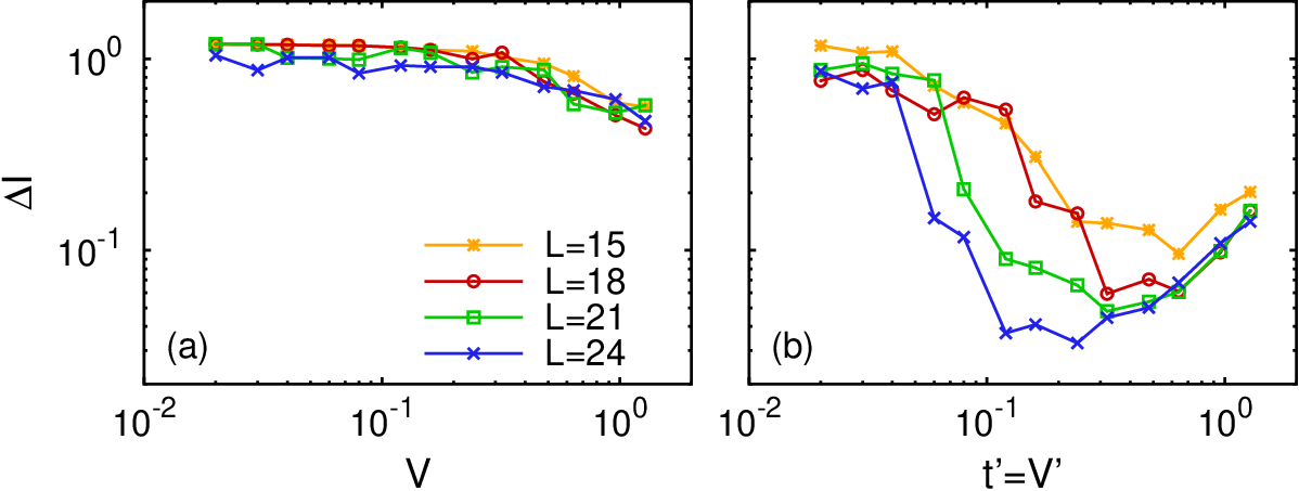
The results obtained for quenches type II imply that they will lead to thermalization in integrable systems. This occurs even though the distribution of conserved quantities is a nontrivial one (it is not flat, which was the case in Refs. [11, 12]). Beyond its implication for the quantum dynamics of integrable systems, one could think of using this information to learn about complicated many-body systems. It implies, e.g., that if we know the kinetic energy of a chaotic strongly correlated fermionic system in equilibrium, we could automatically calculate its momentum distribution by computing the momentum distribution function of a system that is in thermal equilibrium in the noninteracting limit with the same energy as the kinetic energy of the strongly correlated one.
VII momentum distributions
In this section, we test whether the conclusion reached in the previous sections, that quenches type I do not exhibit a clear tendency to thermalize with increasing system size while quenches type II do, holds for an observable, the momentum distribution function .
In Fig. 8, we show the momentum distribution function obtained within the diagonal ensemble for various initial states for quenches type I [Figs. 8(a)–8(d)] and type II [Figs. 8(e)–8(h)], and compare them to the momentum distribution functions predicted by the GGE and the GE [52]. That figure shows that while the GGE results closely follow the ones in the DE for all quenches, the GE results are only consistently closer to the DE ones as one increases in quenches type II [Figs. 8(f)–8(h)].

Once again, in order to be more quantitative, we compute the integrated differences between the GE and DE results, namely
| (18) |

Results for are presented in Fig. 9(a) for quenches type I and in Fig. 9(b) for quenches type II. In the former figure, no consistent trend is seen in the with increasing system size. In contrast, in Fig. 9(b) one can see that, for the three largest system sizes, decreases steadily with increasing for between 0.1 and 1. For , but finite, we expect that thermalization will also occur, with the upturn seen in Fig. 9(b) for moving to larger values of as the system size increases [32].
The results obtained for the momentum distribution function are in agreement with what was expected from our previous analysis, and indicates that quenches type II lead to thermalization, while quenches type I do not lead to thermalization or require much larger system sizes to observe an approach to the thermal predictions.
VIII summary
We have studied quenches to an integrable Hamiltonian mappable to free fermions, in which the initial state is selected to be either an eigenstate of an integrable Hamiltonian that is nonmappable to a noninteracting one (quench type I) or an eigenstate of a nonintegrable Hamiltonian (quench type II). By studying weighted energy densities and entropies, we have found no clear evidence that quenches type I, at least within our Hamiltonians of interest and away from the middle of the spectrum, lead to an un-bias sampling of the eigenstates of the final Hamiltonian. Quenches type II, on the other hand, are found to provide such an un-bias sampling. Furthermore, an analysis of different systems sizes indicates that, in the thermodynamic limit, an infinitesimal quench type II will lead to thermalization. Here, an important requirement to keep in mind is that the initial state must be away from the edges of the spectrum. This is because, for systems with two-body interactions in the absence of randomness, chaotic eigenstates can only be found away from the edges of the spectrum [33, 34].
We have also shown that, in the initial state, an analysis of the distribution of the quantities that are conserved after the quench provides an understanding of why thermalization occurs in one type of quenches while it fails in the other one. In quenches type I, that distribution remains different from, or approaches very slowly with increasing systems size, the one in thermal equilibrium after the quench. This implies that an un-bias sampling of the eigenstates of the final Hamiltonian does not occur or takes very large systems to be discerned. The opposite is true for quenches type II. Hence, quenches type II provide a consistent way of creating initial states that have the appropriate distribution of conserved quantities so that thermalization can occur after a quench to integrability. Special initial states for which this occurred in quenches type I were discussed in Refs. [11, 12]. However, the distribution of conserved quantities in those cases was (trivially) flat corresponding to infinite temperature systems after the quench.
Finally, by studying the momentum distribution function in quenches type I and type II, we have shown that the conclusions reached on the basis of the results for the energy distributions, entropies, and conserved quantities hold. Namely, we have found no indications that quenches type I lead to the thermalization of this observable while quenches type II do result in thermal behavior.
Acknowledgements.
This work was supported by the U.S. Office of Naval Research. We are grateful to F. M. Izrailev and L. F. Santos for useful comments on the manuscript.References
- [1] M. A. Cazalilla, R. Citro, T. Giamarchi, E. Orignac, and M. Rigol, Rev. Mod. Phys. 83, 1405 (2011).
- [2] T. Kinoshita, T. Wenger, and D. Weiss, Nature 440, 900 (2006).
- [3] M. Gring, M. Kuhnert, T. Langen, T. Kitagawa, B. Rauer, M. Schreitl, I. Mazets, D. A. Smith, E. Demler, and J. Schmiedmayer, Science 337, 1318 (2012).
- [4] S. Trotzky, Y.-A. Chen, A. Flesch, I. P. McCulloch, U. Schollwöck, J. Eisert, and I. Bloch, Nature Phys. 8, 325 (2012).
- [5] M. Rigol, V. Dunjko, and M. Olshanii, Nature 452, 854 (2008).
- [6] M. Rigol, Phys. Rev. Lett. 103, 100403 (2009a).
- [7] M. Rigol, Phys. Rev. A 80, 053607 (2009b).
- [8] M. Rigol, V. Dunjko, V. Yurovsky, and M. Olshanii, Phys. Rev. Lett. 98, 050405 (2007).
- [9] M. Rigol, A. Muramatsu, and M. Olshanii, Phys. Rev. A 74, 053616 (2006).
- [10] A. C. Cassidy, C. W. Clark, and M. Rigol, Phys. Rev. Lett. 106, 140405 (2011).
- [11] M. Rigol and M. Fitzpatrick, Phys. Rev. A 84, 033640 (2011).
- [12] K. He and M. Rigol, Phys. Rev. A 85, 063609 (2012).
- [13] M. A. Cazalilla, Phys. Rev. Lett. 97, 156403 (2006).
- [14] A. Iucci and M. A. Cazalilla, Phys. Rev. A 80, 063619 (2009).
- [15] A. Iucci and M. A. Cazalilla, New J. Phys. 12, 055019 (2010).
- [16] M.-C. Chung, A. Iucci, and M. A. Cazalilla, New J. Phys. 14, 075013 (2012).
- [17] P. Calabrese and J. Cardy, J. Stat. Mech. p. P06008 (2007).
- [18] M. Kollar and M. Eckstein, Phys. Rev. A 78, 013626 (2008).
- [19] M. Cramer, C. M. Dawson, J. Eisert, and T. J. Osborne, Phys. Rev. Lett. 100, 030602 (2008).
- [20] T. Barthel and U. Schollwöck, Phys. Rev. Lett. 100, 100601 (2008).
- [21] D. Rossini, A. Silva, G. Mussardo, and G. E. Santoro, Phys. Rev. Lett. 102, 127204 (2009).
- [22] D. Rossini, S. Suzuki, G. Mussardo, G. E. Santoro, and A. Silva, Phys. Rev. B 82, 144302 (2010).
- [23] J. Mossel and J.-S. Caux, New J. Phys. 12, 055028 (2010).
- [24] D. Fioretto and G. Mussardo, New J. Phys. 12, 055015 (2010).
- [25] P. Calabrese, F. H. L. Essler, and M. Fagotti, Phys. Rev. Lett. 106, 227203 (2011).
- [26] P. Calabrese, F. H. L. Essler, and M. Fagotti, J. Stat. Mech. 2012, P07022 (2012a).
- [27] P. Calabrese, F. H. L. Essler, and M. Fagotti, J. Stat. Mech. 2012, P07016 (2012b).
- [28] E. T. Jaynes, Phys. Rev. 106, 620 (1957a).
- [29] E. T. Jaynes, Phys. Rev. 108, 171 (1957b).
- [30] J. M. Deutsch, Phys. Rev. A 43, 2046 (1991).
- [31] M. Srednicki, Phys. Rev. E 50, 888 (1994).
- [32] M. Rigol and M. Srednicki, Phys. Rev. Lett. 108, 110601 (2012).
- [33] L. F. Santos and M. Rigol, Phys. Rev. E 81, 036206 (2010a).
- [34] L. F. Santos and M. Rigol, Phys. Rev. E 82, 031130 (2010b).
- [35] L. F. Santos, F. Borgonovi, and F. M. Izrailev, Phys. Rev. Lett. 108, 094102 (2012a).
- [36] L. F. Santos, F. Borgonovi, and F. M. Izrailev, Phys. Rev. E 85, 036209 (2012b).
- [37] V. V. Flambaum, F. M. Izrailev, and G. Casati, Phys. Rev. E 54, 2136 (1996).
- [38] V. V. Flambaum and F. M. Izrailev, Phys. Rev. E 55, R13 (1997a).
- [39] V. V. Flambaum and F. M. Izrailev, Phys. Rev. E 56, 5144 (1997b).
- [40] V. V. Flambaum and F. M. Izrailev, Phys. Rev. E 61, 2539 (2000).
- [41] T. Holstein and H. Primakoff, Phys. Rev. 58, 1098 (1940).
- [42] P. Jordan and E. Wigner, Z. Phys. 47, 631 (1928).
- [43] M. Rigol and A. Muramatsu, Phys. Rev. A 70, 031603(R) (2004).
- [44] M. Rigol and A. Muramatsu, Phys. Rev. A 72, 013604 (2005).
- [45] K. He and M. Rigol, Phys. Rev. A 83, 023611 (2011).
- [46] M. Rigol, Phys. Rev. A 72, 063607 (2005).
- [47] H. Fang and Y. Saad, SIAM Journal on Scientific Computing 34, A2220 (2012).
- [48] A. Polkovnikov, Ann. Phys. 326, 486 (2011).
- [49] L. F. Santos, A. Polkovnikov, and M. Rigol, Phys. Rev. Lett. 107, 040601 (2011).
- [50] M. Rigol, Phys. Rev. A 82, 037601 (2010).
- [51] We are interested in understanding what happens in the thermodynamic limit for quenches that may have arbitrarily large but finite [] values of or . This ensures that the ratio between the width of the weighted energy density distribution after the quench and the width of the full energy spectrum vanishes in the thermodynamic limit [5]. Hence, here we are not concerned with what happens for a finite system as or is increased to arbitrarily large values.
- [52] We have also computed the momentum distribution functions within the CE. Those results, as well as their differences with the ones obtained within the DE and the GGE, are not only qualitatively but also quantitatively very similar to the ones discussed here for the GE. This is expected from the finite size scaling analysis of this observable in the CE and the GE presented in Ref. [46].