Non-unital non-Markovianity of quantum dynamics

Understanding and characterizing general features of the dynamics of open quantum systems is of great importance to physics, chemistry, and biology [1]. The non-Markovian character is one of the most central aspects of an open quantum process, and attracts increasing attentions [2, 3, 4, 6, 7, 8, 9, 11, 13, 12, 15, 14, 10, 5, 16]. Markovian dynamics of quantum systems is described by a quantum dynamical semigroup [1, 17], and often taken as an approximation of realistic circumstances with some very strict assumptions. Meanwhile, exact master equations, which describe the non-Markovian dynamics, are complicated [9]. Based on the infinitesimal divisibility in terms of quantum dynamical semigroup, Wolf et al. provided a model-independent way to study the non-Markovian features [3, 2]. Later, in the intuitive picture of the backward information flow leading to the increasing of distinguishability in intermediate dynamical maps, Breuer, Laine, and Piilo (BLP) proposed a measure on the degree of non-Markovian behavior based on the monotonicity of the trace distance under quantum channels [4], as shown in Fig. 1. The BLP non-Markovianity has been widely studied, and applied in various models [18, 20, 21, 22, 19, 23].

Unlike for classical stochastic processes, the non-Markovian criteria for quantum processes is non-unique, and even controversial. First, the non-Markovian criteria from the infinitesimal divisibility and the backward information flow are not equivalent [19, 20]. Second, several other non-Markovianity measures, based on different mechanism like the monotonicity of correlations under local quantum channels, have been introduced [6, 13]. Third, even in the framework of backward information flow, trace distance is not the unique monotone distance for the distinguishability between quantum states. Other monotone distances on the space of density operators can be found in Ref. [24], and the statistical distance [25, 26] is another widely-used one. Different distance should not be expected to give the same non-Markovian criteria. The inconsistency among various non-Markovianity reflects different dynamical properties.

In this paper, we show that the BLP non-Markovianity cannot reveal the infinitesimal non-divisibility of quantum processes caused by the non-unital part of the dynamics. Besides non-Markovianity, “non-unitality” is another important dynamical property, which is the necessity for the increasing of the purity $\mathrm{Tr\rho^{2}}$ under quantum channels [27] and for the creating of quantum discord in two-qubit systems under local quantum channels [28]. In the same spirit as BLP non-Markovianity, we define a measure on the non-unitality. As BLP non-Markovianity is the most widely used measure on non-Markovianity, we also provide a measure on the non-unital non-Markovianity, which can be conveniently used as a supplement to the BLP measure, when the quantum process is non-unital. We also give an example to demonstrate an extreme case, where the BLP non-Markovianity vanishes while the quantum process is not infinitesimal divisible.

This paper is organized as follows. In Sec. II, we give a brief review on the representation of density operators and quantum channels with Hermitian orthonormal operator basis, and various measures on non-Markovianity. In Sec. III, we investigate the non-unitality and the non-unital non-Markovianity and give the corresponding quantitative measures respectively. In Sec. IV, we apply the non-unital non-Markovianity measure on a family of quantum processes, which are constructed from the generalized amplitude damping channels. Section V is the conclusion.

The non-Markovianity measure $\mathcal{N}_{\mathrm{BLP}}$ is available to capture the non-Markovian behavior of the unital aspect of the dynamics. But for the non-unital aspect, it is not capable. To show this, we use the Hermitian orthonormal operator basis to express states and quantum channels. Utilizing Eq. (5), the trace distance between two states $\rho_{1}$ and $\rho_{2}$ is given by

Therefore, for the two evolving states, we get

where $\rho_{1}$, $\rho_{2}$ are initial states of the system.

From this equation one can see that the trace distance between any two evolved states is irrelevant to the non-unital part $\mathbf{c}(\mathcal{E}_{t})$ of the time evolution. Then if there are two quantum channels, whose affine maps are $\mathbf{r}\mapsto M\mathbf{r}+\mathbf{c}_{1}$ and $\mathbf{r}\mapsto M\mathbf{r}+\mathbf{c}_{2}$, respectively, the characteristic of trace distance between the evolving states from any two initial states cannot distinguish these two channels. More importantly, $\mathbf{c}(\mathcal{E}_{t})$ may cause the non-divisibility of the quantum process $\mathcal{E}_{t}$, and this cannot be revealed by $\mathcal{N}_{\mathrm{BLP}}$.

On the other hand, the non-unital part $\mathbf{c}(\mathcal{E}_{t})$ has its own physical meaning: $\mathbf{c}(\mathcal{E}_{t})\neq 0$ is necessary for the increasing of the purity $\mathcal{P}(\rho)=\mathrm{Tr}(\rho^{2})$ [27]. In other words,

Besides the non-Markovian feature, the non-unitality is another kind of general feature of quantum processes. In analogy to the definition of BLP non-Markovianity, we defined the following measure on the degree of the non-unitality of a quantum process:

where $\rho_{0}$ is the initial state. Obviously, $N_{\mathrm{nu}}(\mathcal{E}_{t})$ vanishes if $\mathbf{c}(\mathcal{E}_{t})=0$.

Since the non-unital aspect of the dynamics, which is not revealed by the trace distance, has its own speciality, we aim to measure the effect of non-unitality on non-Markovian behavior. However, a perfect separation of the non-unital aspect from the total non-Markovianity may be infeasible. Therefore we require a weak version $\mathcal{N}_{\mathrm{nu}}$ for measuring non-unital non-Markovianity to satisfy the following three conditions: (i) $\mathcal{N}_{\text{nu}}$ vanishes if $\mathcal{E}_{t}$ is infinitesimal divisible, (ii) $\mathcal{N}_{\text{nu}}$ vanishes if $\mathcal{E}_{t}$ is unital, (iii) $\mathcal{N}_{\mathrm{nu}}$ should be relevant to $\mathbf{c}(\mathcal{E}_{t})$. Based on these conditions, we introduce the following measure

where $\mathcal{X}:=\left\{\varrho_{\tau}\mid 0\leq\tau\leq\infty\right\}$ with $\varrho_{\tau}:=\mathcal{E}_{\tau}(\openone/d)$ is the set of the trajectory states which evolve from the maximally mixed state, and

with $D(\rho_{1},\rho_{2})$ an appropriate distance which will be discussed below. The first condition is guaranteed if we require that $D$ is monotone under any CPT maps, i.e., $D[\mathcal{E}(\rho_{1}),\mathcal{E}(\rho_{2})]\leq D(\rho_{1},\rho_{2})$ for any quantum channel $\mathcal{E}$. For the unital time evolution, the set $\mathcal{X}=\{\openone/d\}$ only contains the maximally mixed state, so the above defined $\mathcal{N}_{\mathrm{nu}}$ vanishes, and the second condition is satisfied. The third condition excludes the trace distance.

In this paper, we use the Bures distance which is defined as

where

is the Uhlmann fidelity [38, 39] between $\rho_{1}$ and $\rho_{2}$. Here $|O|=\sqrt{O^{\dagger}O}$. Bures distance is an appropriate distance for $\mathcal{N}_{\mathrm{nu}}$ because it obeys the monotonicity under CPT maps [24] and is relevant to $\mathbf{c}(\mathcal{E}_{t})$. As here only the monotonicity of distance is relevant, for simplicity, we can also take the square of the Bures distance or just the opposite value of Unlmann fidelity as a simple version of monotone “distance” [12]. Quantum relative entropy [40] $S(\rho_{1}\|\rho_{2})=\text{Tr}\left[\rho_{1}(\ln\rho_{1}-\ln\rho_{2})\right]$, or its symmetric version $S_{\mathrm{sym}}(\rho_{1}\|\rho_{2}):=S(\rho_{1}\|\rho_{2})+S(\rho_{2}\|\rho_{1})$, is another qualified candidate for the distance. Noting that when the support of $\rho_{1}$ is not within the support of $\rho_{2}$, namely, $\mathrm{supp}(\rho_{1})\nsubseteq\mathrm{supp(\rho_{2})}$, $S(\rho_{1}\|\rho_{2})$ will be infinite, so in such cases, quantum relative entropy will bring singularity to the measure of non-Markovianity. Also, Hellinger distance [41] is qualified. Although all of these distances are monotone under CPT maps, they may have different characteristics in the same dynamics, see Ref. [42].

The difference between non-unital non-Markovian measure defined by Eq. (26) and the BLP-type measures, including those which use other alternative distances, is the restriction on the pairs of initial states. Comparing with the BLP-type measures relying on any pair of initial states, the non-unital non-Markovianity measure only relies on the pairs consisting of the maximally mixed state and its trajectory states. On one hand, this restriction makes the non-unital non-Markovianity measure vanish when the quantum processes are unital, no matter they are Markovian or non-Markovian; on the other hand, this restriction reflects that non-unital non-Markovianity measure reveals only a part of information concerning the non-Markovian behaviors.

To illustrate the non-unital non-Markovian behavior, we give an example in this section. We use the generalized amplitude damping channel (GADC) as a prototype to construct a quantum process. The GADC can be described by $\mathcal{E}(\rho)=\sum_{i}E_{i}\rho E_{i}^{\dagger}$ with the Kraus operators $\{E_{i}\}$ given by [43, 37]

where $p$ and $\eta$ are real parameters. Note that for any $p\in[0,1]$ and any $\eta\in[0,1]$, the corresponding $\mathcal{E}$ is a quantum channel. For a two-level system, the Hermitian orthonormal operator basis can be chosen as $\bm{\lambda}=\bm{\sigma}/\sqrt{2}$, where $\bm{\sigma}=\{\sigma_{x},\sigma_{y},\sigma_{z}\}$ is the vector of Pauli matrices. With the decomposition in Eq. (5), the affine map for the Bloch vector is given by $\mathbf{r}(\mathcal{E}(\rho))\mapsto M(\mathcal{E})\mathbf{r}(\rho)+\mathbf{c}(\mathcal{E})$ [37], where

The GADC is unital if and only if $p=1/2$ or $\eta=1$. When $\eta=1$, $M(\mathcal{E})=\openone$, the map is identity.

A quantum process can be constructed by making the parameter $p$ and $\eta$ to be dependent on time $t$. For simplicity, we take $p_{t}=\cos^{2}\omega t$ and $\eta_{t}=e^{-t}$, where $\omega$ is a constant real number. This is a legitimate quantum process, because $\mathcal{E}_{t}$ is a quantum channel for every $t\geq 0$, and $\mathcal{E}_{t=0}$ is the identity map.

First, let us consider the $\mathcal{N}_{\mathrm{BLP}}$ for this quantum process. For any two initial states $\rho_{1}$ and $\rho_{2}$, we have the trace distance

where $|\mathbf{r}|=\sqrt{\mathbf{r}\cdot\mathbf{r}}$ is the Euclidean length of the vector $\mathbf{r}$, and we used the equality

for Pauli matrices. Denoting $\mathbf{r}(\rho_{1})-\mathbf{r}(\rho_{2})$ by $(x,y,z)^{\mathrm{T}}$, we get

which implies $\frac{\mathrm{d}}{\mathrm{d}t}D_{\mathrm{tr}}\left[\mathcal{E}_{t}(\rho_{1}),\mathcal{E}_{t}(\rho_{2})\right]\leq 0$ for every time point $t\geq 0$ and for any real numbers $x$, $y$, and $z$. Thus, the BLP non-Markovianity vanishes, i.e., $\mathcal{N}_{\mathrm{BLP}}(\mathcal{E}_{t})\equiv 0$, although $\mathcal{E}_{t}$ may be not infinitesimal divisible, which will become clear later.

In order to investigate whether $\mathcal{E}_{t}$ is infinitesimal divisible or not, we shall apply $\mathcal{N}_{\mathrm{nu}}$ in the above model. The trajectory of the maximally mixed state under $\mathcal{E}_{t}$ reads

where

Taking these trajectory states as the initial states, we get the corresponding evolving states:

Then the fidelity reads

where

To compare with the behavior of trace distance, we also get $D_{\mathrm{tr}}\left[\mathcal{E}_{t}(\varrho_{0}),\mathcal{E}_{t}(\varrho_{\tau})\right]=\left|\eta_{t}W_{\tau}\right|/2$. With the expressions $\eta_{t}=e^{-t}$ and $p_{t}=\cos^{2}\omega t$, it is

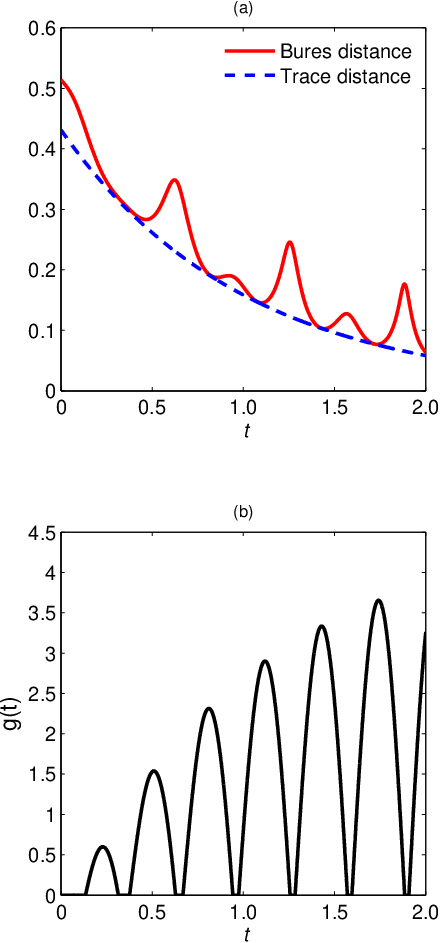
In Fig. 2(a), we can see that while the trace distance between the evolving states $\mathcal{E}_{t}(\varrho_{0})$ and $\mathcal{E}_{t}(\varrho_{\tau})$ monotonously decreases with the time $t$, the Bures distance increases during some intermediate time intervals. From Eq. (59), one can see although $D_{\mathrm{tr}}[\mathcal{E}_{t}(\varrho_{0}),\mathcal{E}_{t}(\varrho_{\tau})]$ depends on $W_{\tau}$, it does not depend on $W_{t}$. Actually, from Eq. (49) one could find that for any two initial states, the trace distance between the evolving states is independent on $W_{t}$. In this sense, the BLP non-Markovianity treats a family of quantum processes, which only differ with $p_{t}$, as the same one. Meanwhile, $\mathcal{N}_{\mathrm{nu}}$ reveals the effects of $p_{t}$ on the infinitesimal non-divisibility and is capable of measuring it.

In order to compare with BHP measure, we also calculate the $g(t)$ defined by Eq. (21). We get

with

The mediate dynamical maps $\mathcal{E}_{t+\epsilon,t}$ with infinitesimal $\epsilon$ are not completely positive when $g(t)>0$. From Fig. 2(b), we can see that the increasing of the Bures distance occurs in the regimes where $g(t)>0$, which coincides with the monotonicity of Bures distance under CPT maps.

In conclusion, we have shown that the measure for non-Markovianity based on trace distance cannot reveal the infinitesimal non-divisibility caused by the non-unital part of the dynamics. In order to reflect effects of the non-unitality, we have constructed a measure on the non-unital non-Markovianity, and also defined a measure on the non-unitality, in the same spirit as BLP non-Markovianity measure.

Like non-Markovianity, the non-unitality is another interesting feature of the quantum dynamics. With the development of quantum technologies, we need novel theoretical approaches for open quantum systems. It is expected that some quantum information methods would help us to understand some generic features of quantum dynamics. We hope this work may draw attention to study more dynamical properties from the informational perspective.