跳到论文正文
W Papers独立论文阅读器 arXiv:1301.5574 论文正文 计算阅读时间 · 0%
引用这篇论文根据当前论文元数据生成,正式投稿前建议核对。


License: arXiv.org perpetual non-exclusive license
arXiv:1301.5574v1 [math-ph] 23 Jan 2013

From the Micro-scale to Collective Crowd Dynamics.

Nicola Bellomo ††thanks: Department of Mathematics, Politecnico Torino Corso Duca degli Abruzzi 24, 10129 Torino, Italy, (nicola.bellomo@polito.it). Partially supported by MIUR, Italian Minister for University and Research    Abdelghani Bellouquid ††thanks: University Cadi Ayyad, Ecole Nationale des Sciences Appliquées, Safi, Morocco,(bellouq2002@yahoo.fr). Supported by Hassan II Academy of Sciences and Technology (Morocco), Project “Méthodes mathématiques et outils de modélisation et simulation pour le cancer”    Damian Knopoff ††thanks: Facultad de Matemática, Astronomía y Física, University of Cordoba, CIEM-CONICET Córdoba, Argentina,(damianknopoff@gmail.com).
Abstract

This paper deals with the kinetic theory modeling of crowd dynamics with the aim of showing how the dynamics at the micro-scale is transferred to the dynamics of collective behaviors. The derivation of a new model is followed by a qualitative analysis of the initial value problem. Existence of solutions is proved for arbitrary large times, while simulations are developed by computational schemes based on splitting methods, where the transport equations treated by finite difference methods for hyperbolic equations. Some preliminary reasonings toward the modeling of panic conditions are proposed.

Key words: Crowd dynamics, complexity, scaling, living systems, nonlinear interactions.

1 Introduction

The modeling of pedestrian crowd dynamics can be developed at different representation scales, namely micro- and macro-scales with the intermediate approach of the kinetic theory, where the dependent variable is a probability distribution over the micro-state of pedestrians. The interested reader is addressed to the review paper [6], where the existing literature is reviewed and critically analyzed focusing at different modeling scales. Namely, at the micro-scale by ordinary differential equations, see among others [18, 20, 21]; at the macro-scale obtained by the classical approach by conservation equations, among others [10, 24]; or by stochastic models related to evolving probability measure [26]. The interplay between individual-based and macroscopic models is studied in [13]. Additional bibliography and conceptual links with the modeling of vehicular traffic are proposed in [5]. A detailed analysis of empirical data is delivered by various papers [9, 27, 30] among others.

This present paper specifically refers to [3], where the main hint, further stressed in [6], is that the modeling approach should retain, as far as it is possible, the complexity features of crowds to be viewed as a living, hence complex, system. This paper presents an introduction to modeling where pedestrians move with only velocity modulus and change their velocity directions both due to interactions with other pedestrians and to the search of their specific target, for instance the exit zone. This present paper shows how the dynamics at the micro-scale of pedestrians is transferred to the dynamics of collective behaviors. Modeling and simulations include interactions between pedestrian that move toward different targets, while their dynamics can be induced, by signals from the outer environment to an exit direction. A qualitative analysis of the initial value problem, and some sample simulations are presented.

The approach developed in this paper is based on the methods of the kinetic theory of active particles, which shows the ability to retain various complexity features. This approach has been applied to the modeling of several living systems as documented, among others, in the modeling of vehicular traffic [4, 8], swarms [7], social competition [1], and migration phenomena [23].

The contents are proposed through four additional sections. In details, Section 2 presents the mathematical model obtained as a development of that given in [3] to include the dynamics on the velocity modulus and interactions of pedestrians that move toward different directions [2]. Section 3 introduces the problem of existence of solutions to the initial value problem in unbounded domains and announces the existence theorems for arbitrary large times. The technical proofs are developed in Sections 4 and 5. Simulations obtained by application of the splitting method, are presented in Section 6 with a detailed computational analysis of the dynamics of the moving boundary of the domain occupied by the crowd. Finally, the last section first critically analyzes the use of the kinetic theory approach and subsequently looks ahead to research perspectives focusing on the modeling panic conditions.

2 A Mathematical Model

Let us consider a large system of pedestrians moving in a bounded domain Ω⊆𝑹2\Omega\subseteq\mbox{\boldmath$R$}^{2}, which may include, as shown in Figure 1, internal obstacles. The boundary of Ω\Omega is denoted by ∂Ω\partial\Omega. The modeling approach also refers to unbounded domains in two space dimensions. Pedestrians can be subdivided into two different groups, moving toward two different targets, denoted by T1T_{1} and T2T_{2}, respectively.

Refer to caption
Figure 1: – Geometry of the domain Ω\Omega: Pedestrians enter from II and can move towards two different targets: pedestrians at PP and at QQ move to T2T_{2} and T1T_{1}, respectively.
Refer to caption Refer to caption
(a) (b)
Figure 2: (a) Interaction domain for an individual in the position 𝐱{\mathbf{x}}. (b) Interaction between a candidate particle in the position PP moving in the direction θh\theta_{h} and a field particle in QQ moving in the direction θp\theta_{p}; θν\theta_{\nu} is the angle from PP to the target TT.

A preliminary step of the derivation of the model, following [3], consists in the assessment of the representation of the system according to the methods of the generalized kinetic theory. This means selecting the microscopic state of the individual state of the pedestrians and of the probability distributions over such state. Two distributions are considered, corresponding to the aforesaid groups of pedestrians pursuing different objectives, which are the dependent variables of the equation modeling the overall dynamics of the system.

Bearing all above in mind, the microscopic state can be defined by the variables: position 𝐱={x,y}∈Ω⊆𝑹2{\mathbf{x}}=\{x,y\}\in\Omega\subseteq\mbox{\boldmath$R$}^{2}, and speed 𝐯∈Dv⊆𝑹2{\mathbf{v}}\in D_{v}\subseteq\mbox{\boldmath$R$}^{2}. Dimensionless coordinates are used by dividing space coordinates by the largest dimension ℓ\ell of Ω\Omega, while the velocity modulus vv is referred to the largest admissible velocity vℓv_{\ell} that can be reached by a speedy pedestrian in optimal conditions of the ambient where the crowd moves.

Polar coordinates with discrete values are used for the velocity variable 𝐯={v,θ}{\mathbf{v}}=\{v,{\theta}\}, where vv is the velocity modulus and θ{\theta} identifies the velocity directions with respect to the xx-axis:

Iθ={θ1=0,…,θi,…,θn=nn−1​2​π},I_{\theta}=\{{\theta}_{1}=0\,,\ldots\,,{\theta}_{i}\,,\ldots\,,{\theta}_{n}=\frac{n}{n-1}2\pi\},
Iv={v1=0,…,vj,…,vm=1}.\quad I_{v}=\{v_{1}=0\,,\ldots\,,v_{j}\,,\ldots\,,v_{m}=1\}.

Out of this discrete velocity representation some specific cases can be considered. For instance the case of two different groups, labeled with the superscript σ=1,2\sigma=1,2, which move towards two different targets. Moreover, if the activity variable is assumed to be homogenously distributed for all pedestrians, the corresponding representation is as follows:

fσ​(t,𝐱,𝐯,u)=∑i=1n∑j=1mfi​jσ​(t,𝐱)​δ​(θ−θi)⊗δ⁡(v−vj)⊗δ⁡(u−u0),f^{\sigma}(t,{\mathbf{x}},{\mathbf{v}},u)=\sum_{i=1}^{n}\sum_{j=1}^{m}f_{ij}^{\sigma}(t,{\mathbf{x}})\,\delta({\theta}-{\theta}_{i})\otimes\delta(v-v_{j})\otimes\delta(u-u_{0})\,, (1)

where fi​jσ​(t,𝐱)=fσ​(t,𝐱,θi,vj,u0)f_{ij}^{\sigma}(t,{\mathbf{x}})=f^{\sigma}(t,{\mathbf{x}},{\theta}_{i},v_{j},u_{0}) corresponding, for each group σ=1,2{\sigma}=1,2, to the i​jij-particle, namely to the pedestrian moving in the direction θi{\theta}_{i} with velocity vjv_{j}.

Macroscopic quantities are obtained by weighted sums. In particular, the number density and flow of pedestrians are, respectively, given by:

ρ⁡(t,𝐱)=∑σ=12ρσ​(t,𝐱)=∑σ=12∑i=1n∑j=1mfi​jσ​(t,𝐱),\rho(t,{\mathbf{x}})=\sum_{{\sigma}=1}^{2}\rho^{\sigma}(t,{\mathbf{x}})=\sum_{{\sigma}=1}^{2}\sum_{i=1}^{n}\sum_{j=1}^{m}f_{ij}^{\sigma}(t,{\mathbf{x}})\,, (2)

and

𝐪(t,𝐱)=∑σ=12𝐪σ(t,𝐱)=∑σ=12∑i=1n∑j=1m(vjcosθi,vjsinθi)fi​jσ(t,𝐱).{\mathbf{q}}(t,{\mathbf{x}})=\sum_{{\sigma}=1}^{2}{\mathbf{q}}^{\sigma}(t,{\mathbf{x}})=\sum_{{\sigma}=1}^{2}\sum_{i=1}^{n}\sum_{j=1}^{m}\left(v_{j}\,\cos{\theta}_{i}\,,v_{j}\,\sin{\theta}_{i}\,\right)f_{ij}^{\sigma}(t,{\mathbf{x}}). (3)

Remark 2.1. The use of discrete space microscopic states was introduced in [15] and [12] to model the granular behavior of vehicular traffic, namely it is observed in [14] that the number of vehicles is not large enough to justify the assumption of a continuous distribution function. The same reasonings are valid also in the case of pedestrians in a crowd.

Remark 2.2. The more general case, where the activity variable is heterogeneously distributed and is modified by interactions is critically analyzed in the last section focusing on the modeling of panic conditions.

The derivation of models needs to be related to a mathematical structure suitable to retain, as far as possible, the complexity of crowds dynamics. Accordingly, the following qualitative features of the dynamics are taken into account:

i) Pedestrians have a visibility zone Λ=Λ⁡(𝐱)\Lambda=\Lambda({\mathbf{x}}), see Figure 2(a), which does not coincide with the whole domain Ω\Omega due to the limited visibility angle of each individual. The specific geometry of Ω\Omega can reduce the visibility zone for pedestrians near walls.

ii) Interactions, at each at time tt, involve: the test (i​j)(ij)-particle, which is representative of the whole system; field (p​q)(pq)-particles in 𝐱∗{\mathbf{x}}^{*} of the visibility zone Λ\Lambda; and candidate pedestrian (h​k)(hk), in 𝐱{\mathbf{x}}. The candidate pedestrian modifies, in probability, its state into that of the test pedestrian, due to interactions with the field pedestrians, while the test pedestrian losses its state due to interactions with the field pedestrians. The activity of the candidate pedestrian is uwu_{w}, which is not modified by the interaction.

iii) The output of interactions is modeled, by using tools of the game theory [28, 29], by the discrete probability density function 𝒜h​k,p​qσ​(i​j){\cal A}_{hk,pq}^{\sigma}(ij), which denotes the probability that a candidate (h​k)(hk)-particle modifies its state into that of the test (i​j)(ij)-particle due to interaction with the field (p​q)(pq)-particles. The transition density depends on the whole local number density ρ\rho.

iv) The frequency of the interactions is modeled by the term η\eta that is allowed to depend on the density of the field particles in the visibility zone.

Time and space dynamics of the distribution function fi​jσf_{ij}^{\sigma} can be obtained by equating its increase on time in the elementary volume of the space of the microscopic states to the net flow into such volume due to transport and interactions:

(∂t\displaystyle\big(\partial_{t} +\displaystyle+ 𝐯i​j⋅∂𝐱)fi​jσ(t,𝐱)=𝒥[𝐟](t,𝐱)\displaystyle{\mathbf{v}}_{ij}\cdot\partial_{\bf x}\big)f_{ij}^{\sigma}(t,{\mathbf{x}})={\cal J}[{\mathbf{f}}](t,{\mathbf{x}})\hfill (4)
=\displaystyle= ∑h,p=1n∑k,q=1m∫Λη⁡[ρ⁡(t,𝐱∗)]​𝒜h​k,p​qσ​(i​j)​[ρ⁡(t,𝐱∗)]​fh​kσ​(t,𝐱)​fp​qσ​(t,𝐱∗)​d​𝐱∗\displaystyle\sum_{h,p=1}^{n}\sum_{k,q=1}^{m}\int_{\Lambda}\eta[\rho(t,{\mathbf{x}}^{*})]{\cal A}_{hk,pq}^{\sigma}(ij)[\rho(t,{\mathbf{x}}^{*})]f_{hk}^{\sigma}(t,{\mathbf{x}})\,f_{pq}^{\sigma}(t,{\mathbf{x}}^{*})\,d{\mathbf{x}}^{*}
0000\displaystyle 0000 −\displaystyle- fi​jσ​(t,𝐱)​∑p=1n∑q=1m∫Λη⁡[ρ⁡(t,𝐱∗)]​fp​qσ​(t,𝐱∗)​d​𝐱∗,\displaystyle f_{ij}^{\sigma}(t,{\mathbf{x}})\sum_{p=1}^{n}\sum_{q=1}^{m}\int_{\Lambda}\eta[\rho(t,{{\mathbf{x}}}^{*})]\,f_{pq}^{\sigma}(t,{\mathbf{x}}^{*})\,d{\mathbf{x}}^{*}, (5)

where 𝐟={fi​j}{\mathbf{f}}=\{f_{ij}\}, while the term 𝒜h​k,p​qσ​(i​j){\cal A}_{hk,pq}^{\sigma}(ij) should be consistent with the probability density property:

∑i=1n∑j=1m𝒜h​k,p​qσ​(i​j)=1,∀h​p∈{1,…,n},∀k​q∈{1,…,m},\sum_{i=1}^{n}\sum_{j=1}^{m}{\cal A}_{hk,pq}^{\sigma}(ij)=1,\quad\forall\,hp\in\{1,\ldots,n\},\quad\forall\,kq\in\{1,\ldots,m\}\,, (6)

for σ=1,2{\sigma}=1,2, and for all conditioning local density. The derivation of specific models can take advantage of the above structures and is obtained by modeling the various terms that appear in Eq. (5). The modeling necessarily needs heuristic assumptions towards the interpretation of the complex phenomenology of the system under consideration.

∙\bullet Interaction rate: The modeling of the term η\eta, can be developed similarly to the case of vehicular traffic [8], by increasing the interaction rate with increasing local density in the free and congested regimes. For higher densities, when pedestrians are obliged to stop, one may assume that η\eta keeps a constant value, or may decay for lack of interest. The following model can be proposed among various conceivable ones:

η⁡(ρ⁡(t,𝐱))=η0​(1+ρ⁡(t,𝐱))​exp⁡(−ρ⁡(t,𝐱)),\eta(\rho(t,{\mathbf{x}}))=\eta^{0}(1+\rho(t,{\mathbf{x}}))\exp\big(-\rho(t,{\mathbf{x}})\big)\,, (7)

while a simpler model can be obtained by assuming η=η0\eta=\eta^{0}.

∙\bullet Transition probability density: The modeling of the transition probability density 𝒜h​k,p​qσ​(i​j){\cal A}_{hk,pq}^{\sigma}(ij) refers to the interactions involving candidate and field particles. The approach proposed here is based on the assumption that particles are subject to three different influences, namely the trend to the exit point, the influence of the stream induced by the other pedestrians, and the selection of the path with minimal density gradient. A simplified interpretation of the phenomenological behavior is obtained by assuming the factorization of the two probability densities modeling the modifications of the velocity direction and modulus:

𝒜h​k,p​qσ​(i​j)=ℬh​pσ​(i)​(θh→θi|ρ⁡(t,𝐱))×𝒞k​qσ​(j)​(vk→vj|ρ⁡(t,𝐱)),{\cal A}_{hk,pq}^{\sigma}(ij)={\cal B}_{hp}^{\sigma}(i)\big({\theta}_{h}\to{\theta}_{i}|\rho(t,{\mathbf{x}})\big)\times{\cal C}_{kq}^{\sigma}(j)\big(v_{k}\to v_{j}|\rho(t,{\mathbf{x}})\big), (8)

where subscripts correspond to the state of the interacting pairs, superscripts to the group and the output of the interaction is indicated in the argument, which depends on the local density.

Remark 2.3. Equation (8) is based on an heuristic assumption that cannot be justified by theoretical issues. However, it simplifies the modeling approach by separating the various causes that modify the dynamics. This assumption does not imply factorization of the probability density due to the mixing action of the variable ρ\rho.

Bearing this remark in mind, let us consider, separately the modeling of the two probability densities:

– Modeling ℬh​pσ​(i):{\cal B}^{\sigma}_{hp}(i): Let us consider the candidate particle in the position PP moving in the direction θh{\theta}_{h} and interacting with a field particle with direction θp{\theta}_{p}. Moreover, let θν{\theta}_{\nu} be the angle from PP to TσT_{{\sigma}} or to the direction of the shortest path, see Figure 2(b). Let us introduce a parameter ασ{\alpha}_{\sigma}, which models the sensitivity of pedestrians both to reach the target TσT_{\sigma}, and to follow the stream. Moreover, it is assumed that the sensitivity to the target, depends on the ratio of vacuum 1−ρ1-\rho, while the sensitivity to the stream depends on the density ρ\rho. Finally it is assumed that the dynamics is more active for higher values of the activity variable u0u_{0}. It is natural that an active individual shows a higher ability to modify the direction of the motion. The games modeling interactions are the same for both groups being understood that the target chased by pedestrians differs for each of them. This qualitative description can be formalized as follows:

– Interaction with a upper stream and target directions, namely θp>θh,θν>θh{\theta}_{p}>{\theta}_{h},\quad{\theta}_{\nu}>{\theta}_{h}: It is assumed that, in addition to the selection of the path with minimal gradients, both actions contribute to an anticlockwise rotation:

ℬh​pσ​(i)\displaystyle{\cal B}^{\sigma}_{hp}(i) =\displaystyle= ασ​u0​(1−ρ)+ασ​u0​ρifi=h+1,\displaystyle{\alpha}_{\sigma}\,u_{0}(1-\rho)+{\alpha}_{\sigma}\,u_{0}\,\rho\quad\hbox{if}\quad i=h+1\,,
ℬh​pσ​(i)\displaystyle{\cal B}^{\sigma}_{hp}(i) =\displaystyle= 1−ασ​u0​(1−ρ)−ασ​u0​ρifi=h,\displaystyle 1-{\alpha}_{\sigma}\,u_{0}(1-\rho)-{\alpha}_{\sigma}\,u_{0}\,\rho\quad\hbox{if}\quad i=h\,,
ℬh​pσ​(i)\displaystyle{\cal B}^{\sigma}_{hp}(i) =\displaystyle= 0ifi=h−1.\displaystyle 0\quad\hbox{if}\quad i=h-1\,.

Analogous calculations can be done for the other cases. The result is as follows:

– Interaction with a upper stream and low target direction θp>θh;θν<θh{\theta}_{p}>{\theta}_{h};\quad{\theta}_{\nu}<{\theta}_{h}:

ℬh​pσ​(i)\displaystyle{\cal B}_{hp}^{\sigma}(i) =\displaystyle= ασ​u0​ρifi=h+1,\displaystyle{\alpha}_{\sigma}\,u_{0}\,\rho\quad\hbox{if}\quad i=h+1\,,
ℬh​pσ​(i)\displaystyle{\cal B}_{hp}^{\sigma}(i) =\displaystyle= 1−ασ​u0​(1−ρ)−ασ​u0​ρifi=h,\displaystyle 1-{\alpha}_{\sigma}\,u_{0}(1-\rho)-{\alpha}_{\sigma}\,u_{0}\,\rho\quad\hbox{if}\quad i=h\,,
ℬh​pσ​(i)\displaystyle{\cal B}_{hp}^{\sigma}(i) =\displaystyle= ασ​u0​(1−ρ)ifi=h−1.\displaystyle{\alpha}_{\sigma}\,u_{0}\,(1-\rho)\quad\hbox{if}\quad i=h-1\,.

– Interaction with a lower stream and upper target direction θp<θh;θν>θh{\theta}_{p}<{\theta}_{h};\quad{\theta}_{\nu}>{\theta}_{h}:

ℬh​pσ​(i)\displaystyle{\cal B}_{hp}^{\sigma}(i) =\displaystyle= ασ​u0​(1−ρ)ifi=h+1,\displaystyle{\alpha}_{\sigma}\,u_{0}(1-\rho)\quad\hbox{if}\quad i=h+1\,,
ℬh​pσ​(i)\displaystyle{\cal B}_{hp}^{\sigma}(i) =\displaystyle= 1−ασ​u0​(1−ρ)−ασ​u0​ρifi=h,\displaystyle 1-{\alpha}_{\sigma}\,u_{0}(1-\rho)-{\alpha}_{\sigma}\,u_{0}\,\rho\quad\hbox{if}\quad i=h\,,
ℬh​pσ​(i)\displaystyle{\cal B}_{hp}^{\sigma}(i) =\displaystyle= ασ​u0​ρifi=h−1.\displaystyle{\alpha}_{\sigma}\,u_{0}\,\rho\quad\hbox{if}\quad i=h-1\,.

– Interaction with a lower stream and target directions θp<θh;θν<θh{\theta}_{p}<{\theta}_{h};\quad{\theta}_{\nu}<{\theta}_{h}:

ℬh​pσ​(i)\displaystyle{\cal B}_{hp}^{\sigma}(i) =\displaystyle= 0ifi=h+1,\displaystyle 0\quad\hbox{if}\quad i=h+1\,,
ℬh​pσ​(i)\displaystyle{\cal B}_{hp}^{\sigma}(i) =\displaystyle= 1−ασ​u0​(1−ρ)−ασ​u0​ρifi=h,\displaystyle 1-{\alpha}_{\sigma}\,u_{0}(1-\rho)-{\alpha}_{\sigma}\,u_{0}\,\rho\quad\hbox{if}\quad i=h\,,
ℬh​pσ​(i)\displaystyle{\cal B}_{hp}^{\sigma}(i) =\displaystyle= ασ​u0​(1−ρ)+ασ​u0​ρifi=h−1.\displaystyle{\alpha}_{\sigma}\,u_{0}\,(1-\rho)+{\alpha}_{\sigma}\,u_{0}\,\rho\quad\hbox{if}\quad i=h-1\,.

Concerning the term 𝒞k​qσ​(j){\cal C}_{kq}^{{\sigma}}(j), the proposed modeling assumes that pedestrians have a trend to adjust each other their velocity modulus, namely an encounter with a faster (slower) pedestrian induces a trend to increase (decrease) the speed. This trend is conditioned by the local density, namely it decreases with increasing density. It is assumed that also this type of dynamics depends on the activity u0u_{0} of the pedestrian and on their sensitivity βσ{\beta}_{\sigma} to the change of velocity. The corresponding table of games, which defines the interaction rules, is as follows:

∙\bullet Interaction with faster (or slower) particles vk<vqv_{k}<v_{q}, or vk>vqv_{k}>v_{q}, respectively

𝒞k​qσ​(j)={1−βσ​u0​ρ,j=k;βσ​u0​ρ,j=k+1;0,otherwise;{\cal C}_{kq}^{{\sigma}}(j)=\left\{\begin{array}[]{ll}1-{\beta}_{\sigma}\,u_{0}\rho,&\hbox{$j=k$;}\\ {\beta}_{\sigma}u_{0}\rho,&\hbox{$j={k+1}$;}\\ 0,&\hbox{otherwise;}\end{array}\right.
𝒞k​qσ​(j)={βσ​u0​ρ,j=k;1−βσ​u0​ρ,j=k−1;0,otherwise.{\cal C}_{kq}^{{\sigma}}(j)=\left\{\begin{array}[]{ll}{\beta}_{\sigma}\,u_{0}\rho,&\hbox{$j=k$;}\\ 1-{\beta}_{\sigma}\,u_{0}\rho,&\hbox{$j={k-1}$;}\\ 0,&\hbox{otherwise.}\end{array}\right.

∙\bullet Interaction with equally fast particles k=qk=q

𝒞k​qσ​(j)={1−2​βσ​u0​ρ,j=k;βσ​u0​ρ,j=k−1;βσ​u0​ρ,j=k+1.{\cal C}_{kq}^{{\sigma}}(j)=\left\{\begin{array}[]{ll}1-2{\beta}_{\sigma}\,u_{0}\rho,&\hbox{$j=k$;}\\ {\beta}_{\sigma}\,u_{0}\rho,&\hbox{$j=k-1$;}\\ {\beta}_{\sigma}\,u_{0}\rho,&\hbox{$j=k+1$.}\end{array}\right.

Moreover,

∙\bullet for k=1k=1 the candidate particle cannot reduce the velocity, while for k=kk=k cannot increase it:

𝒞k​qσ​(j)={1−βσ​u0​ρ,j=1;βσ​u0​ρ,j=2;0,otherwise;{\cal C}_{kq}^{{\sigma}}(j)=\left\{\begin{array}[]{ll}1-{\beta}_{\sigma}\,u_{0}\,\rho,&\hbox{$j=1$;}\\ {\beta}_{\sigma}\,u_{0}\,\rho,&\hbox{$j=2$;}\\ 0,&\hbox{otherwise;}\end{array}\right.
𝒞k​qσ​(j)={βσ​u0​ρ,j=m−1;1−βσ​u0​ρ,j=m;0,otherwise.{\cal C}_{kq}^{{\sigma}}(j)=\left\{\begin{array}[]{ll}{\beta}_{\sigma}\,u_{0}\,\rho,&\hbox{$j=m-1$;}\\ 1-{\beta}_{\sigma}\,u_{0}\,\rho,&\hbox{$j=m$;}\\ 0,&\hbox{otherwise.}\end{array}\right.

∙\bullet The modeling corresponding to jam densities ρ∈[ε,1]\rho\in[{\varepsilon},1] implements that pedestrians reduce to zero their velocity.

Remark 2.4. If the heterogeneous behavior of pedestrians needs to be taken into account a probability distribution over the variable uu has to be introduced with the modeling of the interaction dynamics that modifies it.

3 On the Initial Value Problem

The initial value problem consists in solving Eqs. (5) with initial conditions given by

fi​jσ​(0,𝐱)=ϕi​jσ​(𝐱).f_{ij}^{\sigma}(0,{\mathbf{x}})=\phi_{ij}^{\sigma}({\mathbf{x}}). (9)

Let us introduce the mild form obtained by integrating along the characteristics:

fi​jσ^​(t,𝐱)\displaystyle\widehat{f_{ij}^{\sigma}}(t,{\mathbf{x}}) =\displaystyle= ϕi​jσ​(𝐱)+∫0t(Γi​jσ^​[𝐟,𝐟]​(s,𝐱)−fi​jσ^​(s,𝐱)​L⁡[𝐟]^​(s,𝐱))​𝑑s,\displaystyle\phi_{ij}^{\sigma}({\mathbf{x}})+\int_{0}^{t}\bigg(\widehat{\Gamma_{ij}^{\sigma}}[{\mathbf{f}},{\mathbf{f}}](s,{\mathbf{x}})-\widehat{f_{ij}^{\sigma}}(s,\,{\mathbf{x}})\widehat{L[{\mathbf{f}}]}(s,\,{\mathbf{x}})\bigg)ds, (10)
i∈{1,…,n},j∈{1,…,m},σ∈{1,2},\displaystyle\quad i\in\{1,\ldots,n\},\quad\,j\in\{1,\ldots,m\},\quad\sigma\in\{1,2\},

where the following notation has been used for any given vector f⁡(t,𝐱)f(t,{\mathbf{x}}): fi​jσ^​(t,𝐱)=fi​jσ​(t,x+vj​cos⁡(θi)​t,y+vj​sin⁡(θi)​t)\widehat{f_{ij}^{\sigma}}(t,{\mathbf{x}})=f_{ij}^{\sigma}(t,x+v_{j}\cos({\theta}_{i})t,y+v_{j}\sin({\theta}_{i})t), and where the operators in (10) are defined as follows:

Γi​jσ​[𝐟,𝐟]^\displaystyle\widehat{\Gamma_{ij}^{\sigma}[{\mathbf{f}},{\mathbf{f}}]} (t,𝐱)=∑h,p=1n∑k,q=1m∫Λη⁡[ρ⁡(t,𝐱∗)]​𝒜h​k,p​qσ​(i​j)​[ρ⁡(t,𝐱∗)]\displaystyle(t,{\mathbf{x}})=\sum_{h,p=1}^{n}\sum_{k,q=1}^{m}\int_{\Lambda}\eta[\rho(t,{\mathbf{x}}^{*})]{\cal A}_{hk,pq}^{{\sigma}}(ij)[\rho(t,{\mathbf{x}}^{*})] (11)
fh​kσ^\displaystyle\widehat{f_{hk}^{{\sigma}}} (t,x+(vj​cos⁡(θi)−vk​cos⁡(θh))​t,y+(vj​sin⁡(θi)−vk​sin⁡(θh))​t)\displaystyle(t,x+(v_{j}\cos({\theta}_{i})-v_{k}\cos({\theta}_{h}))t,y+(v_{j}\sin({\theta}_{i})-v_{k}\sin({\theta}_{h}))t)\,
fp​qσ^\displaystyle\widehat{f_{pq}^{{\sigma}}} (t,x∗−vq​cos⁡(θp)​t,y∗−vq​sin⁡(θp)​t)​d​𝐱∗,\displaystyle(t,x^{*}-v_{q}\cos({\theta}_{p})t,y^{*}-v_{q}\sin({\theta}_{p})t)\,d{\mathbf{x}}^{*},

and

L⁡[𝐟]^​(t,𝐱)=∑p=1n∑q=1m∫Λη⁡[ρ⁡(t,𝐱∗)]​fp​qσ^​(t,x∗−vq​cos⁡(θp)​t,y∗−vq​sin⁡(θp)​t)​d​𝐱∗,\widehat{L[{\mathbf{f}}]}(t,\,{\mathbf{x}})=\sum_{p=1}^{n}\sum_{q=1}^{m}\int_{\Lambda}\eta[\rho(t,{{\mathbf{x}}}^{*})]\,\widehat{f_{pq}^{\sigma}}(t,x^{*}-v_{q}\cos({\theta}_{p})t,y^{*}-v_{q}\sin({\theta}_{p})t)\,d{\mathbf{x}}^{*}, (12)

where 𝐟={fi​jσ}{\mathbf{f}}=\{f_{ij}^{\sigma}\}.

Let us now define the following functional space:

LM2​n,2​m1={f=(fi​jσ)∈M2​n,2​m:∥f∥1=∑σ=12∑i=1n∑j=1m∫Ω∣fi​jσ(t,𝐱)∣d𝐱<∞}L^{1}_{M_{2n,2m}}=\{f=(f_{ij}^{\sigma})\in M_{2n,2m}:\parallel f\parallel_{1}=\sum_{\sigma=1}^{2}\sum_{i=1}^{n}\sum_{j=1}^{m}\int_{\Omega}\mid f_{ij}^{\sigma}(t,{\mathbf{x}})\mid\,d{\mathbf{x}}<\infty\}

and introduce, for T>0T>0, the Banach space

XT=X⁡[0,T]=C⁡([0,T],LM2​n,2​m1)X_{T}=X[0,T]=C([0,T],L^{1}_{M_{2n,2m}})

of the matrix-valued functions f=f⁡(t,𝐱):[0,T]×Ω→M2​n,2​m.f=f(t,{\mathbf{x}}):[0,T]\times\Omega\rightarrow M_{2n,2m}. such that for all fixed t∈[0,T]t\in[0,T] the function 𝐱→f⁡(t,𝐱){\mathbf{x}}\rightarrow f(t,{\mathbf{x}}) belongs to LM2​n,2​m1L^{1}_{M_{2n,2m}}, where the norm in XTX_{T} is given by

∥f∥XT=supt∈[0,T]∥f∥1.\parallel f\parallel_{X_{T}}=\sup_{t\in[0,\,T]}\parallel f\parallel_{1}. (13)

The qualitative analysis developed in the following takes advantage of the following assumptions that are consistent with the physics of the system under consideration:

Assumption H.1. For all positive RR, there exists a constant Cη>0C_{\eta}>0 so that

0<η⁡(ρ)≤Cη,whenever0≤ρ≤R.0<\eta(\rho)\leq C_{\eta}\,,\quad\hbox{whenever}\quad 0\leq\rho\leq R\,. (14)

Assumption H.2. Both the encounter rate η⁡[ρ]\eta[\rho] and the transition probability 𝒜h​k,p​qσ​(i​j)​[ρ]{\cal A}_{hk,pq}^{\sigma}(ij)[\rho] are Lipschitz continuous functions of the macroscopic density ρ\rho, i.e., that there exist constants Lη,L𝒜L_{\eta},L_{\mathcal{A}} such that

{∣η⁡[ρ1]−η⁡[ρ2]∣≤Lη​∣ρ1−ρ2∣,∣𝒜h​k,p​qσ​(i​j)​[ρ1]−𝒜h​k,p​qσ​(i​j)​[ρ2]∣≤L𝒜​∣ρ1−ρ2∣,\left\{\begin{array}[]{l}\displaystyle{\mid\eta[\rho_{1}]-\eta[\rho_{2}]\mid\leq L_{\eta}\mid\rho_{1}-\rho_{2}\mid},\\ \\ \displaystyle{\mid{\cal A}_{hk,pq}^{\sigma}(ij)[\rho_{1}]-{\cal A}_{hk,pq}^{\sigma}(ij)[\rho_{2}]\mid\leq L_{\mathcal{A}}\mid\rho_{1}-\rho_{2}\mid},\end{array}\right.

whenever 0≤ρ1≤R0\leq\rho_{1}\leq R, 0≤ρ2≤R0\leq\rho_{2}\leq R, and all i,h,p=1,..,ni,h,p=1,..,n and j,k,q=1,..,mj,k,q=1,..,m.

The following results can be proved under assumptions H..1 and H.2:

Theorem 3.1

(Local Existence) Let ϕi​jσ∈L∞∩L1\phi_{ij}^{\sigma}\in L_{\infty}\cap L^{1}, ϕi​jσ≥0\phi_{ij}^{\sigma}\geq 0, then there exists ϕ0\phi^{0} so that, if ∥ϕ∥1≤ϕ0\parallel\phi\parallel_{1}\leq\phi^{0}, there exist TT, a0a_{0}, and RR so that a unique non-negative solution to the initial value problem of Eqs.(5)–(9) exists and satisfies:

f∈XT,supt∈[0,T]∥f(t)∥1≤a0∥ϕ∥1,f\in X_{T},\qquad\sup_{t\in[0,T]}\parallel f(t)\parallel_{1}\leq a_{0}\parallel\phi\parallel_{1}, (15)

and

ρ⁡(t,𝐱)≤R,∀t∈[0,T],𝐱∈Ω.\rho(t,{\mathbf{x}})\leq R,\quad\forall t\in[0,T],\quad{\mathbf{x}}\in\Omega\,. (16)

Moreover, if

∑σ=12∑i=1n∑j=1m∥ϕi​jσ∥∞≤1,\sum_{\sigma=1}^{2}\sum_{i=1}^{n}\sum_{j=1}^{m}\parallel\phi_{ij}^{\sigma}\parallel_{\infty}\leq 1\,, (17)

and ∥ϕ∥1\parallel\phi\parallel_{1} is small, one has

ρ⁡(t,𝐱)≤1,∀t∈[0,T],𝐱∈Ω.\rho(t,{\mathbf{x}})\leq 1,\quad\forall t\in[0,T],\quad{\mathbf{x}}\in\Omega. (18)
Theorem 3.2

(Global Existence) Under the assumptions of Theorem 3.1, there exist ϕr\phi^{r}, (r=1,…,p−1)(r=1,...,p-1) such that if ∥ϕ∥1≤ϕr\parallel\phi\parallel_{1}\leq\phi^{r}, there exists ara_{r} so that it is possible to find a unique non-negative solution to the initial value problem of Eqs.(5)–(9) satisfying for any r≤p−1r\leq p-1

f⁡(t)∈X⁡[0,(p−1)​T],f(t)\in X[0,(p-1)T], (19)
supt∈[0,T]∥f(t+(r−1)T)∥1≤ar−1∥ϕ∥1,\sup_{t\in[0,T]}\parallel f(t+(r-1)T)\parallel_{1}\leq a_{r-1}\parallel\phi\parallel_{1}, (20)

and

ρ⁡(t+(r−1)​T,𝐱)≤R,∀t∈[0,T],𝐱∈Ω.\rho(t+(r-1)T,{\mathbf{x}})\leq R,\quad\forall t\in[0,T],\quad{\mathbf{x}}\in\Omega. (21)

Moreover, if ϕ\phi satisfies (17), one has

ρ⁡(t+(r−1)​T,𝐱)≤1,∀t∈[0,T],𝐱∈Ω.\rho(t+(r-1)T,{\mathbf{x}})\leq 1,\quad\forall t\in[0,T],\quad{\mathbf{x}}\in\Omega. (22)

4 Proof of Theorem 3.1 (Local Existence)

Let us introduce the function

ψi​jσ​(t,𝐱)=exp⁡(λ​t)​fi​jσ​(t,𝐱),forλ>0.\psi_{ij}^{\sigma}(t,{\mathbf{x}})=\exp(\lambda t)f_{ij}^{\sigma}(t,{\mathbf{x}})\,,\quad\hbox{for}\quad\lambda>0\,. (23)

Therefore, system (5)-(9) can be written in equivalent form in terms of the functions ψ⁡(t,x)=(ψi​jσ​(t,x))\psi(t,x)=(\psi_{ij}^{\sigma}(t,x)), where ψi​jσ\psi_{ij}^{\sigma} are solutions of the following mild problem:

ψi​jσ^​(t,𝐱)\displaystyle\widehat{\psi_{ij}^{\sigma}}(t,{\mathbf{x}}) =\displaystyle= ϕi​jσ​(𝐱)+∫0t(Γi​jσ​[ψ,ψ]^​(s,𝐱)​exp⁡(−λ​s)CLOSE\displaystyle\phi_{ij}^{\sigma}({\mathbf{x}})+\int_{0}^{t}\bigg(\widehat{\Gamma_{ij}^{\sigma}[\psi,\psi]}(s,{\mathbf{x}})\exp(-\lambda s) (24)
+\displaystyle+ OPENψi​jσ^​(s,𝐱)​{λ−L⁡[ψ]^​(s,𝐱)​exp⁡(−λ​s)})​d​s.\displaystyle\displaystyle\widehat{\psi_{ij}^{\sigma}}(s,\,{\mathbf{x}})\bigg\{\lambda-\widehat{L[\psi]}(s,\,{\mathbf{x}})\exp(-\lambda s)\bigg\}\bigg)ds.

Moreover, let us consider the operator AA acting on XTX_{T} whose components are

A​(ψ)i​jσ^​(t,𝐱)\displaystyle\widehat{A(\psi)_{ij}^{\sigma}}(t,{\mathbf{x}}) =\displaystyle= ϕi​jσ​(𝐱)+∫0t(Γi​jσ​[ψ,ψ]^​(s,𝐱)​exp⁡(−λ​s)CLOSE\displaystyle\phi_{ij}^{\sigma}({\mathbf{x}})+\int_{0}^{t}\bigg(\widehat{\Gamma_{ij}^{\sigma}[\psi,\psi]}(s,{\mathbf{x}})\exp(-\lambda s) (25)
+\displaystyle+ OPENψi​jσ^​(s,𝐱)​{λ−L⁡[ψ]^​(s,𝐱)​exp⁡(−λ​s)})​d​s.\displaystyle\displaystyle\widehat{\psi_{ij}^{\sigma}}(s,\,{\mathbf{x}})\bigg\{\lambda-\widehat{L[\psi]}(s,\,{\mathbf{x}})\exp(-\lambda s)\bigg\}\bigg)ds.

The principle of contractive mapping can be applied to Eq.(25). However, the proof is based on various sharp inequalities that are preliminary proved in the following Lemmas.

Lemma 4.1

Let T>0T>0, ψ∈XT\psi\in X_{T}, then A​ψ∈XTA\psi\in X_{T} and ∃C1>0\exists C_{1}>0 so that

∥A(ψ)∥XT≤∥ϕ∥1+C1λ∥ψ∥XT2+λT∥ψ∥XT.\parallel A(\psi)\parallel_{X_{T}}\leq\parallel\phi\parallel_{1}+{C_{1}\over\lambda}\parallel\psi\parallel_{X_{T}}^{2}+\lambda T\parallel\psi\parallel_{X_{T}}. (26)

Proof of Lemma 4.1: To prove the estimate (26), we need first to estimate the nonlinear operators Γi​jσ^​[ψ,ψ]\widehat{\Gamma_{ij}^{\sigma}}[\psi,\psi] and L⁡[ψ]^\widehat{L[\psi]} in L1L_{1}. Taking into account the assumption H.1 on η\eta yields

∥Γi​jσ^[ψ,ψ]∥1\displaystyle\parallel\widehat{\Gamma_{ij}^{\sigma}}[\psi,\psi]\parallel_{1} ≤\displaystyle\leq Cη∑h,p=1n∑k,q=1m∫Λ𝒜h​k,p​qσ(ij)[ρ(t,𝐱∗]\displaystyle C_{\eta}\sum_{h,p=1}^{n}\sum_{k,q=1}^{m}\int_{\Lambda}{\cal A}_{hk,pq}^{\sigma}(ij)[\rho(t,{\mathbf{x}}^{*}] (27)
×\displaystyle\times ∣ψp​qσ^​(t,x∗−vq​cos⁡(θp)​t,y∗−vq​sin⁡(θp)​t)∣​d​𝐱∗\displaystyle\mid\widehat{\psi_{pq}^{\sigma}}(t,x^{*}-v_{q}\cos({\theta}_{p})t,y^{*}-v_{q}\sin({\theta}_{p})t)\mid\,d{\mathbf{x}}^{*}
×\displaystyle\times ∫Ω|ψh​kσ^​(t,x+(vj​cos⁡(θi)−vk​cos⁡(θh))​t,yCLOSE\displaystyle\int_{\Omega}\mid\widehat{\psi_{hk}^{\sigma}}(t,x+(v_{j}\cos({\theta}_{i})-v_{k}\cos({\theta}_{h}))t,y
+\displaystyle+ OPEN(vj​sin⁡(θi)−vk​sin⁡(θh))​t)|d​𝐱.\displaystyle(v_{j}\sin({\theta}_{i})-v_{k}\sin({\theta}_{h}))t)\mid\,d{\mathbf{x}}.

Using Eq. (6) on the probability density 𝒜h​k,p​qσ​(i​j){\cal A}_{hk,pq}^{\sigma}(ij) and the following transformations with jacobian equal one

𝐱=(x,y)↦(x−vq​cos⁡(θp)​t,y−vq​sin⁡(θp)​t),{\mathbf{x}}=(x,y)\mapsto(x-v_{q}\cos({\theta}_{p})t,y-v_{q}\sin({\theta}_{p})t),
𝐱=(x,y)↦(x+(vj​cos⁡(θi)−vk​cos⁡(θh))​t,y+(vj​sin⁡(θi)−vk​sin⁡(θh))​t),{\mathbf{x}}=(x,y)\mapsto(x+(v_{j}\cos({\theta}_{i})-v_{k}\cos({\theta}_{h}))t,y+(v_{j}\sin({\theta}_{i})-v_{k}\sin({\theta}_{h}))t),

yields:

∥Γ^[ψ,ψ]∥1=∑σ=12∑i,j∥Γi​jσ^[ψ,ψ]∥1≤Cη∥ψ∥12.\parallel\widehat{\Gamma}[\psi,\psi]\parallel_{1}=\sum_{\sigma=1}^{2}\sum_{i,j}\parallel\widehat{\Gamma_{ij}^{\sigma}}[\psi,\psi]\parallel_{1}\leq C_{\eta}\parallel\psi\parallel_{1}^{2}. (28)

Moreover, the same estimate can be obtained for the loss operator L^\widehat{L}:

∥L⁡[ψ]^ψ^∥1≤Cη∥ψ∥12.\parallel\widehat{L[\psi]}\widehat{\psi}\parallel_{1}\leq C_{\eta}\parallel\psi\parallel_{1}^{2}\,. (29)

The following inequality is directly deduced, by using (28)-(29), from (25):

∥A(ψ)∥1≤∥ϕ∥1+2λCη(1−exp(−λt))∥ψ∥XT2+λt∥ψ∥XT,\parallel A(\psi)\parallel_{1}\leq\parallel\phi\parallel_{1}+{2\over\lambda}C_{\eta}(1-\exp(-\lambda t))\parallel\psi\parallel_{X_{T}}^{2}+\lambda\,t\parallel\psi\parallel_{X_{T}},

which gives (26) with C1=2​Cη.C_{1}=2\,C_{\eta}.

Analogous calculations lead to the following inequality:

∥A(ψ)(t)−A(ψ)(s)∥1≤∣t−s∣(C1∥ψ∥XT2+λ∥ψ∥XT),\parallel A(\psi)(t)-A(\psi)(s)\parallel_{1}\leq\mid t-s\mid(C_{1}\parallel\psi\parallel_{X_{T}}^{2}+\lambda\parallel\psi\parallel_{X_{T}})\,,

which gives the continuity of the operator AA in L1L_{1}. Therefore, Lemma 4.1 is proved.   

Lemma 4.2

Let ψ1=(ψi​jσ1)∈L1,ψ2=(ψi​jσ2)∈L1\psi^{1}=({\psi_{ij}^{\sigma}}^{1})\in L_{1},\psi^{2}=({\psi_{ij}^{\sigma}}^{2})\in L_{1}, such that

{∑σ=12∑i=1n∑j=1mψi​jσ1^​(t,x−vj​cos⁡(θi)​t,y−vj​sin⁡(θi)​t)≤R​exp⁡(λ​t),∑σ=12∑i=1n∑j=1mψi​jσ2^​(t,x−vj​cos⁡(θi)​t,y−vj​sin⁡(θi)​t)≤R​exp⁡(λ​t),\left\{\begin{array}[]{l}\displaystyle{\sum_{\sigma=1}^{2}\sum_{i=1}^{n}\sum_{j=1}^{m}}\widehat{{\psi_{ij}^{\sigma}}^{1}}(t,\,x-v_{j}\cos({\theta}_{i})t,y-v_{j}\sin({\theta}_{i})t)\leq R\exp(\lambda t),\\ \\ \displaystyle{\sum_{\sigma=1}^{2}\sum_{i=1}^{n}\sum_{j=1}^{m}}\widehat{{\psi_{ij}^{\sigma}}^{2}}(t,\,x-v_{j}\cos({\theta}_{i})t,y-v_{j}\sin({\theta}_{i})t)\leq R\exp(\lambda t),\end{array}\right.

for x∈Ω,t≥0x\in\Omega,t\geq 0. Then

∥Γ^(ψ1,ψ1)−Γ^(ψ2,ψ2)∥1\displaystyle\parallel\widehat{\Gamma}(\psi^{1},\psi^{1})-\widehat{\Gamma}(\psi^{2},\psi^{2})\parallel_{1} ≤\displaystyle\leq (Cη+n​m​R​(Cη​L𝒜+Lη))\displaystyle(C_{\eta}+nmR(C_{\eta}L_{\mathcal{A}}+L_{\eta})) (30)
×\displaystyle\times (∥ψ1∥1+∥ψ2∥1)∥ψ1−ψ2∥1,\displaystyle(\parallel\psi^{1}\parallel_{1}+\parallel\psi^{2}\parallel_{1})\parallel\psi^{1}-\psi^{2}\parallel_{1}\,,
∥ψ1^Λ^(ψ1)−ψ2^Λ^(ψ2)∥1≤(Cη+LηR)(∥ψ1∥1+∥ψ2∥1)∥ψ1−ψ2∥1.\parallel\widehat{\psi^{1}}\,\widehat{\Lambda}(\psi^{1})-\widehat{\psi^{2}}\,\widehat{\Lambda}(\psi^{2})\parallel_{1}\leq(C_{\eta}+L_{\eta}R)(\parallel\psi^{1}\parallel_{1}+\parallel\psi^{2}\parallel_{1})\parallel\psi^{1}-\psi^{2}\parallel_{1}. (31)

Proof of Lemma 4.2: First write Γi​jσ^​(ψ1,ψ1)​(t,𝐱)−Γi​jσ^​(ψ2,ψ2)​(t,𝐱)\widehat{\Gamma_{ij}^{\sigma}}(\psi^{1},\psi^{1})(t,{\mathbf{x}})-\widehat{\Gamma_{ij}^{\sigma}}(\psi^{2},\psi^{2})(t,{\mathbf{x}}) as follows:

Γi​jσ^​(ψ1,ψ1)​(t,𝐱)−Γi​jσ^​(ψ2,ψ2)​(t,𝐱)\displaystyle\widehat{\Gamma_{ij}^{\sigma}}(\psi^{1},\psi^{1})(t,{\mathbf{x}})-\widehat{\Gamma_{ij}^{\sigma}}(\psi^{2},\psi^{2})(t,{\mathbf{x}})
=∑h,p=1n∑k,q=1m∫Λη⁡[ρψ1​(t,𝐱∗)]​𝒜h​k,p​qσ​(i​j)​[ρψ1​(t,𝐱∗)]\displaystyle\quad=\sum_{h,p=1}^{n}\sum_{k,q=1}^{m}\int_{\Lambda}\eta[\rho_{\psi^{1}}(t,{\mathbf{x}}^{*})]{\cal A}_{hk,pq}^{{\sigma}}(ij)[\rho_{\psi^{1}}(t,{\mathbf{x}}^{*})]
×[ψh​kσ1^(t,x+(vjcos(θi)−vkcos(θh))t,y+(vjsin(θi)−vksin(θh))t)\displaystyle\quad\times\bigg[\widehat{{\psi_{hk}^{\sigma}}^{1}}(t,x+(v_{j}\cos({\theta}_{i})-v_{k}\cos({\theta}_{h}))t,y+(v_{j}\sin({\theta}_{i})-v_{k}\sin({\theta}_{h}))t)\,
×ψp​qσ1^​(t,x∗−vq​cos⁡(θp)​t,y∗−vq​sin⁡(θp)​t)\displaystyle\quad\times\widehat{{\psi_{pq}^{\sigma}}^{1}}(t,x^{*}-v_{q}\cos({\theta}_{p})t,y^{*}-v_{q}\sin({\theta}_{p})t)\,
−ψh​kσ2^​(t,x+(vj​cos⁡(θi)−vk​cos⁡(θh))​t,y+(vj​sin⁡(θi)−vk​sin⁡(θh))​t)\displaystyle\quad-\widehat{{\psi_{hk}^{\sigma}}^{2}}(t,x+(v_{j}\cos({\theta}_{i})-v_{k}\cos({\theta}_{h}))t,y+(v_{j}\sin({\theta}_{i})-v_{k}\sin({\theta}_{h}))t)\,
×ψp​qσ2^(t,x∗−vqcos(θp)t,y∗−vqsin(θp)t)]d𝐱∗\displaystyle\quad\times\widehat{{\psi_{pq}^{\sigma}}^{2}}(t,x^{*}-v_{q}\cos({\theta}_{p})t,y^{*}-v_{q}\sin({\theta}_{p})t)\,\bigg]\,d{\mathbf{x}}^{*}
+∑h,p=1n∑k,q=1m∫Λψh,kσ2^(t,x+(vjcos(θi)−vkcos(θh))t,y\displaystyle\quad+\sum_{h,p=1}^{n}\sum_{k,q=1}^{m}\int_{\Lambda}\widehat{{\psi_{h,k}^{\sigma}}^{2}}(t,x+(v_{j}\cos({\theta}_{i})-v_{k}\cos({\theta}_{h}))t,y
OPEN+(vj​sin⁡(θi)−vk​sin⁡(θh))​t)\displaystyle\quad+(v_{j}\sin({\theta}_{i})-v_{k}\sin({\theta}_{h}))t)
×ψp,qσ2^​(t,x∗−vq​cos⁡(θp)​t,y∗−vq​sin⁡(θp)​t)\displaystyle\quad\times\widehat{{\psi_{p,q}^{\sigma}}^{2}}(t,x^{*}-v_{q}\cos({\theta}_{p})t,y^{*}-v_{q}\sin({\theta}_{p})t)
×[η[ρψ1(t,x∗)]𝒜h​k,p​qσ(ij)[ρψ1(t,x∗)]\displaystyle\quad\times\bigg[\eta[\rho_{\psi^{1}}(t,x^{*})]{\cal A}_{hk,pq}^{{\sigma}}(ij)[\rho_{\psi^{1}}(t,x^{*})]
−η[ρψ2(t,x∗)]𝒜h​k,p​qσ(ij)[ρψ2(t,x∗)]]dx∗\displaystyle\quad-\eta[\rho_{\psi^{2}}(t,x^{*})]{\cal A}_{hk,pq}^{{\sigma}}(ij)[\rho_{\psi^{2}}(t,\,x^{*})]\bigg]dx^{*}
=Ai​jσ+Bi​jσ,\displaystyle\qquad=A_{ij}^{\sigma}+B_{ij}^{\sigma},

Using Assumptions H.1, H.2, and summing over i,j,σi,j,\sigma, yields

∑σ=12∑i=1n∑j=1m∥Ai​jσ∥1\displaystyle\qquad\sum_{\sigma=1}^{2}\sum_{i=1}^{n}\sum_{j=1}^{m}\parallel A_{ij}^{\sigma}\parallel_{1}
≤Cη​∑σ=12∑i=1n∑j=1m∑h,p=1n∑k,q=1m∫Λ×Ω𝒜h​k,p​qσ​(i​j)|ψh,kσ1^​(t,x+(vj​cos⁡(θi)CLOSECLOSE\displaystyle\quad\leq C_{\eta}\sum_{\sigma=1}^{2}\sum_{i=1}^{n}\sum_{j=1}^{m}\sum_{h,p=1}^{n}\sum_{k,q=1}^{m}\int_{\Lambda\times\Omega}{\cal A}_{hk,pq}^{{\sigma}}(ij)\mid\widehat{{\psi_{h,k}^{\sigma}}^{1}}(t,x+(v_{j}\cos({\theta}_{i})
−vkcos(θh))t,y+(vjsin(θi)−vksin(θh))t)∣\displaystyle\quad-v_{k}\cos({\theta}_{h}))t,y+(v_{j}\sin({\theta}_{i})-v_{k}\sin({\theta}_{h}))t)\mid
×|ψp​qσ1^​(t,x∗−vq​cos⁡(θp)​t,y∗−vq​sin⁡(θp)​t)\displaystyle\quad\times\mid\widehat{{\psi_{pq}^{\sigma}}^{1}}(t,x^{*}-v_{q}\cos({\theta}_{p})t,y^{*}-v_{q}\sin({\theta}_{p})t)
−ψp​qσ2^​(t,x∗−vq​cos⁡(θp)​t,y∗−vq​sin⁡(θp)​t)|d​𝐱∗​d​𝐱\displaystyle\quad-\widehat{{\psi_{pq}^{\sigma}}^{2}}(t,x^{*}-v_{q}\cos({\theta}_{p})t,y^{*}-v_{q}\sin({\theta}_{p})t)\mid\,d{\mathbf{x}}^{*}d{\mathbf{x}}
+Cη∑σ=12∑i=1n∑j=1m∑h,p=1n∑k,q=1m∫Λ×Ω𝒜h​k,p​qσ(ij)\displaystyle\quad+C_{\eta}\sum_{\sigma=1}^{2}\sum_{i=1}^{n}\sum_{j=1}^{m}\sum_{h,p=1}^{n}\sum_{k,q=1}^{m}\int_{\Lambda\times\Omega}{\cal A}_{hk,pq}^{{\sigma}}(ij)
×∣ψp​qσ2^​(t,x∗−vq​cos⁡(θp)​t,y∗−vq​sin⁡(θp)​t)∣\displaystyle\quad\times\mid\widehat{{\psi_{pq}^{\sigma}}^{2}}(t,x^{*}-v_{q}\cos({\theta}_{p})t,y^{*}-v_{q}\sin({\theta}_{p})t)\mid
×|ψh,kσ1^​(t,x+(vj​cos⁡(θi)−vk​cos⁡(θh))​t,yCLOSE\displaystyle\quad\times\mid\widehat{{\psi_{h,k}^{\sigma}}^{1}}(t,x+(v_{j}\cos({\theta}_{i})-v_{k}\cos({\theta}_{h}))t,y
OPEN+(vj​sin⁡(θi)−vk​sin⁡(θh))​t)\displaystyle\quad+(v_{j}\sin({\theta}_{i})-v_{k}\sin({\theta}_{h}))t)
−ψh,kσ2^​(t,x+(vj​cos⁡(θi)−vk​cos⁡(θh))​t,yCLOSE\displaystyle\quad-\widehat{{\psi_{h,k}^{\sigma}}^{2}}(t,x+(v_{j}\cos({\theta}_{i})-v_{k}\cos({\theta}_{h}))t,y
OPEN+(vj​sin⁡(θi)−vk​sin⁡(θh))​t)|d​𝐱∗​d​𝐱\displaystyle\quad+(v_{j}\sin({\theta}_{i})-v_{k}\sin({\theta}_{h}))t)\mid\,d{\mathbf{x}}^{*}d{\mathbf{x}}
≤Cη∥ψ1−ψ2∥1(∥ψ1∥1+∥ψ2∥1).\displaystyle\qquad\leq C_{\eta}\parallel\psi^{1}-\psi^{2}\parallel_{1}(\parallel\psi^{1}\parallel_{1}+\parallel\psi^{2}\parallel_{1})\,. (32)

On the other hand, considering that

∣(ρψ1−ρψ2)(t,𝐱∗)∣≤exp(−λt)∑σ=12∑r=1n∑ν=1m∣ψr​νσ1^(t,x∗−vνcos(θr)t,y∗\displaystyle\mid(\rho_{\psi^{1}}-\rho_{\psi^{2}})(t,{\mathbf{x}}^{*})\mid\leq\exp(-\lambda t)\sum_{\sigma=1}^{2}\sum_{r=1}^{n}\sum_{\nu=1}^{m}\mid\widehat{{\psi_{r\nu}^{\sigma}}^{1}}(t,\,x^{*}-v_{\nu}\cos({\theta}_{r})t,y^{*}
−vνsin(θr)t)ψr​νσ2^(t,x∗−vνcos(θr)t,y∗−vνsin(θr)t)∣,\displaystyle\quad-v_{\nu}\sin({\theta}_{r})t)\widehat{{\psi_{r\nu}^{\sigma}}^{2}}(t,\,x^{*}-v_{\nu}\cos({\theta}_{r})t,y^{*}-v_{\nu}\sin({\theta}_{r})t)\mid\,,

and

∑p=1n∑q=1m∣ψp​qσ2^​(t,x∗−vq​cos⁡(θp)​t,y∗−vq​sin⁡(θp)​t)∣≤R​exp⁡(λ​t),\sum_{p=1}^{n}\sum_{q=1}^{m}\mid\widehat{{\psi_{pq}^{\sigma}}^{2}}(t,x^{*}-v_{q}\cos({\theta}_{p})t,y^{*}-v_{q}\sin({\theta}_{p})t)\mid\leq R\exp(\lambda t),

then, using Assumptions H.1-H.2, noting that 𝒜h​k,p​qσ​(i​j)≤1{\cal A}_{hk,pq}^{{\sigma}}(ij)\leq 1, and summing over i,j,σi,j,\sigma, yields:

∑σ=12∑i=1n∑j=1m∥Bi​jσ∥1≤≤nmR(Lη+CηLA)∥ψ2∥1∥ψ1−ψ2∥1\displaystyle\sum_{\sigma=1}^{2}\sum_{i=1}^{n}\sum_{j=1}^{m}\parallel B_{ij}^{\sigma}\parallel_{1}\leq\leq nmR(L_{\eta}+C_{\eta}L_{A})\parallel\psi^{2}\parallel_{1}\parallel\psi^{1}-\psi^{2}\parallel_{1}

which gives, by using (32), the estimate (30).

By the same arguments, from Assumptions H.1, and H.2 one deduces (31) and this completes the proof of Lemma 4.2.   

Lemma 4.3

Let T>0T>0, ψ1=(ψi​jσ1),ψ2=(ψi​jσ2)∈XT\psi^{1}=({\psi_{ij}^{\sigma}}^{1}),\psi^{2}=({\psi_{ij}^{\sigma}}^{2})\in X_{T}, satisfying (4.2) for x∈Ω,t∈[0,T]x\in\Omega,t\in[0,T]. Then:

1. There exists a constant C2>0C_{2}>0 such that

∥A(ψ1)−A(ψ2)∥XT\displaystyle\parallel A(\psi^{1})-A(\psi^{2})\parallel_{X_{T}} ≤\displaystyle\leq (C2λ(∥ψ1∥XT+∥ψ2∥XT)+λT)\displaystyle\bigg({C_{2}\over\lambda}(\parallel\psi^{1}\parallel_{X_{T}}+\parallel\psi^{2}\parallel_{X_{T}})+\lambda T\bigg) (33)
∥ψ1−ψ2∥XT.\displaystyle\parallel\psi^{1}-\psi^{2}\parallel_{X_{T}}\,.

2. If (ψ1)i​jσ≥0{(\psi^{1})}_{ij}^{{\sigma}}\geq 0, then there ∃λ0\exists\lambda_{0} such that if λ≥λ0\lambda\geq\lambda_{0} and if ϕi​jσ≥0\phi_{ij}^{\sigma}\geq 0 one has (A⁡(ψ1))i​jσ^≥0\widehat{(A(\psi^{1}))_{ij}^{\sigma}}\geq 0.

3. Let ϕi​jσ∈L∞\phi_{ij}^{\sigma}\in L^{\infty}, then for RR large enough(R≥R1R\geq R_{1}), there exists TT such that

∑σ=12∑i=1n∑j=1m(A⁡(ψ1))i​jσ^​(t,x−vj​cos⁡(θi)​t,y−vj​sin⁡(θi)​t)≤R​exp⁡(λ​t),\sum_{\sigma=1}^{2}\sum_{i=1}^{n}\sum_{j=1}^{m}\widehat{(A(\psi^{1}))_{ij}^{\sigma}}(t,\,x-v_{j}\cos({\theta}_{i})t,y-v_{j}\sin({\theta}_{i})t)\leq R\exp(\lambda t), (34)

∀t∈[0,T],∀x∈Ω.\forall t\in[0,T],\quad\forall x\in\Omega.

Proof of Lemma 4.3: From (25) and Lemma 4.1, one gets easily (33) with

C2=Cη+n​m​R​(Cη​L𝒜+Lη).C_{2}=C_{\eta}+n\,m\,R(C_{\eta}L_{\mathcal{A}}+L_{\eta}). (35)

Since Γi​jσ^​[ψ1,ψ1]​(t,𝐱)≥0\widehat{\Gamma_{ij}^{\sigma}}[\psi^{1},\psi^{1}](t,{\mathbf{x}})\geq 0 if (ψ1)i,jσ≥0({\psi^{1}})_{i,j}^{\sigma}\geq 0, the nonnegativity of (A⁡(ψ1))i​jσ^\widehat{(A(\psi^{1}))_{ij}^{\sigma}} depend on the possibility to find λ>0\lambda>0 such that

λ−L⁡[ψ1]^​(s,𝐱)​exp⁡(−λ​s)≥0.\lambda-\widehat{L[\psi^{1}]}(s,\,{\mathbf{x}})\exp(-\lambda s)\geq 0. (36)

Noting that from (12) and assumption H.1, one obtains

L⁡[ψ1]^​(t,x)=∑p=1n∑q=1m∫Λη⁡[ρ⁡(t,𝐱∗)]​ψ1p​qσ^​(t,x∗−vq​cos⁡(θp)​t,y∗CLOSE\displaystyle\widehat{L[\psi^{1}]}(t,\,x)=\sum_{p=1}^{n}\sum_{q=1}^{m}\int_{\Lambda}\eta[\rho(t,{{\mathbf{x}}}^{*})]\,\widehat{{\psi^{1}}_{pq}^{\sigma}}(t,x^{*}-v_{q}\cos({\theta}_{p})t,y^{*}
OPEN−vq​sin⁡(θp)​t)​d​𝐱∗≤R​exp⁡(λ​t)​Cη​∣Λ∣.\displaystyle\quad-v_{q}\sin({\theta}_{p})t)\,d{\mathbf{x}}^{*}\leq R\exp(\lambda t)C_{\eta}\mid\Lambda\mid.

The nonnegativity of (A⁡(ψ1))i​jσ^\widehat{(A(\psi^{1}))_{ij}^{\sigma}} is then achieved by choosing λ≥λ0=R​Cη​∣Λ∣\lambda\geq\lambda_{0}=RC_{\eta}\mid\Lambda\mid. To deal with 3) first let see that

Γ^​(ψ1,ψ1)​(t,x−vj​cos⁡(θi)​t,y−vj​sin⁡(θi)​t)\displaystyle\widehat{\Gamma}(\psi^{1},\psi^{1})(t,\,x-v_{j}\cos({\theta}_{i})t,y-v_{j}\sin({\theta}_{i})t)
=∑h,p=1n∑k,q=1m∫Λη⁡[ρ⁡(t,x∗)]​𝒜h​k,p​qσ​(i​j)​[ρ⁡(t,x∗)]\displaystyle\qquad=\sum_{h,p=1}^{n}\sum_{k,q=1}^{m}\int_{\Lambda}\eta[\rho(t,x^{*})]{\cal A}_{hk,pq}^{{\sigma}}(ij)[\rho(t,x^{*})]
×ψ1h,kσ^​(t,x−vk​cos⁡(θh)​t,y−vk​sin⁡(θh)​t)\displaystyle\qquad\times\widehat{{\psi^{1}}_{h,k}^{\sigma}}(t,x-v_{k}\cos({\theta}_{h})t,y-v_{k}\sin({\theta}_{h})t)
×ψ1p,qσ^​(t,x∗−vq​cos⁡(θp)​t,y∗−vq​sin⁡(θp)​t)​d​𝐱∗\displaystyle\qquad\times\widehat{{\psi^{1}}_{p,q}^{\sigma}}(t,x^{*}-v_{q}\cos({\theta}_{p})t,y^{*}-v_{q}\sin({\theta}_{p})t)d{\mathbf{x}}^{*}
≤Cη​R2​exp⁡(2​λ​t)​∫Λd​𝐱∗,≤Cη|Λ|R2​exp⁡(2​λ​t).\displaystyle\qquad\leq C_{\eta}R^{2}\exp(2\lambda t)\int_{\Lambda}d{\mathbf{x}}^{*}\,,\leq C_{\eta}\mid\Lambda\mid R^{2}\exp(2\lambda t). (37)

Then the following estimate is proved:

∑σ=12∑i=1n∑j=1m(A⁡(ψ))i​jσ^​(t,x−vj​cos⁡(θi)​t,y−vj​sin⁡(θi)​t)\displaystyle\sum_{\sigma=1}^{2}\sum_{i=1}^{n}\sum_{j=1}^{m}\widehat{(A(\psi))_{ij}^{\sigma}}(t,\,x-v_{j}\cos({\theta}_{i})t,y-v_{j}\sin({\theta}_{i})t)
≤∑σ=12∑i=1n∑j=1m∥ϕi​jσ∥∞+12​λnmCη∣Λ∣R2(exp(2λt)−1)\displaystyle\quad\leq\sum_{\sigma=1}^{2}\sum_{i=1}^{n}\sum_{j=1}^{m}\parallel\phi_{ij}^{\sigma}\parallel_{\infty}+{1\over 2\lambda}n\,m\,C_{\eta}\mid\Lambda\mid R^{2}(\exp(2\lambda t)-1)
+R⁡(exp⁡(λ​t)−1),\displaystyle\quad+R(\exp(\lambda t)-1)\,,

which gives (34) if

R>∑σ=12∑i=1n∑j=1m∥ϕi​jσ∥∞=R1,R>\sum_{\sigma=1}^{2}\sum_{i=1}^{n}\sum_{j=1}^{m}\parallel\phi_{ij}^{\sigma}\parallel_{\infty}=R_{1}, (38)

and

t≤T=12​λln(1+2​λn​m​Cη​∣Λ∣​R2(R−∑σ=12∑i=1n∑j=1m∥ϕi​jσ∥∞)).t\leq T={1\over{2\lambda}}ln\bigg(1+{2\lambda\over nmC_{\eta}\mid\Lambda\mid R^{2}}(R-\sum_{\sigma=1}^{2}\sum_{i=1}^{n}\sum_{j=1}^{m}\parallel\phi_{ij}^{\sigma}\parallel_{\infty})\bigg)\,. (39)


Lemma 4.4

Let TT given by (39) with λ=R​Cη​∣Λ∣\lambda=RC_{\eta}\mid\Lambda\mid (R≥R1)(R\geq R_{1}). Then then there exists ϕ0,R2\phi_{0},R_{2} such that if ∥ϕ∥1≤ϕ0\parallel\phi\parallel_{1}\leq\phi_{0}, R≥R2R\geq R_{2} one has

(λT−1)2≥4​Cλ∥ϕ∥1,(\lambda T-1)^{2}\geq{4C\over\lambda}\parallel\phi\parallel_{1}\,, (40)

where C=M​a​x​(C1,C2)C=Max(C_{1},C_{2}) is given by (4) and (35).

Proof of Lemma 4.4: Using the inequality l​n​(1+x)≤x,x≥0ln(1+x)\leq x,x\geq 0, then one has:

λ​T≤λn​m​Cη​∣Λ∣​R=1n​m​,\lambda T\leq{\lambda\over nmC_{\eta}\mid\Lambda\mid R}={1\over nm}\raise 2.0pt\hbox{,}

which yields

(λT−1)2≥(n​m−1n​m)2⋅(\lambda T-1)^{2}\geq\bigg({nm-1\over nm}\bigg)^{2}\cdotp (41)

Then, if ϕ\phi and RR are such that

∥ϕ∥1≤(n​m−1)28​(n​m)3Cη​∣Λ∣(Cη​L𝒜+Lη)=ϕ0,\parallel\phi\parallel_{1}\leq{(nm-1)^{2}\over 8(nm)^{3}}{C_{\eta}\mid\Lambda\mid\over(C_{\eta}L_{\mathcal{A}}+L_{\eta})}=\phi_{0}, (42)

and

R≥8∣Λ∣∥ϕ∥1(n​m)2(n​m−1)2=R2.R\geq{8\over\mid\Lambda\mid}\parallel\phi\parallel_{1}{(nm)^{2}\over(nm-1)^{2}}=R_{2}. (43)

Then (40) is proved. This completes the proof.   

Now we have all tools for the proof of the local existence theorem.

Proof of Theorem 3.1: Let us consider the following subset in XTX_{T} defined as follows:

BT={ψ=(ψi​jσ)∈XT:ψi​jσ≥0,∥ψ(t)∥1≤a0∥ϕ∥1,\displaystyle B_{T}=\{\psi=(\psi_{ij}^{\sigma})\in X_{T}:\psi_{ij}^{\sigma}\geq 0,\parallel\psi(t)\parallel_{1}\leq a_{0}\parallel\phi\parallel_{1},\,
∑σ=12∑i=1n∑j=1mψi​jσ^​(t,x−vj​cos⁡(θi)​t,y−vj​sin⁡(θi)​t)\displaystyle\sum_{\sigma=1}^{2}\sum_{i=1}^{n}\sum_{j=1}^{m}\widehat{\psi_{ij}^{\sigma}}(t,\,x-v_{j}\cos({\theta}_{i})t,y-v_{j}\sin({\theta}_{i})t)
≤Rexp(λt),t∈[0,T],x∈Ω}.\displaystyle\quad\leq R\exp(\lambda t),t\in[0,T],x\in\Omega\}.

Let ψ1,ψ2∈BT\psi^{1},\psi^{2}\in B_{T}, and let R≥R0=M​a​x​(R1,R2)R\geq R_{0}=Max(R_{1},R_{2}) then from Lemma 4.3, there exists TT such that (A⁡(ψ1))i​jσ^≥0\widehat{(A(\psi^{1}))_{ij}^{\sigma}}\geq 0 and satisfying (34) for λ=R​Cη​∣Λ∣\lambda=RC_{\eta}\mid\Lambda\mid, t∈[0,T]t\in[0,T]. Moreover from Lemmas 4.1 and 4.3, one has:

∥A(ψ1)∥XT≤∥ϕ∥1+1λCa02∥ϕ∥12+λa0T∥ϕ∥1,\parallel A(\psi^{1})\parallel_{X_{T}}\leq\parallel\phi\parallel_{1}+{1\over\lambda}Ca_{0}^{2}\parallel\phi\parallel_{1}^{2}+\lambda a_{0}T\parallel\phi\parallel_{1}, (44)

and

∥A(ψ1)−A(ψ2)∥XT≤(2λCa0∥ϕ∥1+λT)∥ψ1−ψ2∥XT,\parallel A(\psi^{1})-A(\psi^{2})\parallel_{X_{T}}\leq\bigg({2\over\lambda}Ca_{0}\parallel\phi\parallel_{1}+\lambda T\bigg)\parallel\psi^{1}-\psi^{2}\parallel_{X_{T}}, (45)

where CC is the constants defined in Lemma 4.4. Let

Δ0=(λT−1)2−4​Cλ∥ϕ∥1.\Delta_{0}=(\lambda T-1)^{2}-{4C\over\lambda}\parallel\phi\parallel_{1}. (46)

Then by the previous Lemma one has Δ0≥0\Delta_{0}\geq 0, for ∥ϕ∥1≤ϕ0\parallel\phi\parallel_{1}\leq\phi_{0}. Let now a0a_{0} be the positive quantity given by:

a0=λ​(1−λ​T)−Δ02C∥ϕ∥1​,a_{0}=\lambda\,{(1-\lambda T)-\sqrt{\Delta_{0}}\over 2C\parallel\phi\parallel_{1}}\raise 2.0pt\hbox{,} (47)

which is a solution of

∥ϕ∥1+1λCa02∥ϕ∥12+λa0T∥ϕ∥1=a0∥ϕ∥1.\parallel\phi\parallel_{1}+{1\over\lambda}Ca_{0}^{2}\parallel\phi\parallel_{1}^{2}+\lambda a_{0}T\parallel\phi\parallel_{1}=a_{0}\parallel\phi\parallel_{1}\,.

That shows from (44) that A⁡(ψ1)∈BTA(\psi^{1})\in B_{T}. Moreover

(2λCa0∥ϕ∥1+λT)=1−Δ0<1\bigg({2\over\lambda}\,C\,a_{0}\parallel\phi\parallel_{1}+\lambda\,T\bigg)=1-\sqrt{\Delta_{0}}<1

which shows from (45) that the mapping AA is a contraction in a ball BTB_{T}, and application of the fixed point theorem gives the proof of Theorem 3.1, which refers to local existence. Moreover, if ϕ\phi satisfies (17), and if ∥ϕ∥1\parallel\phi\parallel_{1} is very small, then from (38) and (43), one can choose RR such that (18) can be obtained. This completes the proof.   

5 Proof of Existence for Large times

The aim of this section consists in proving Theorem 3.2 concerning the global existence of solutions to the initial value problem for Eqs.(5)-(9). It will be proved that the solution can be extended in each interval [0,p​T][0,pT], for p∈Np\in N. As in the preceding section some preliminary results are needed:

Lemma 5.1

Let ϕ\phi satisfy the conditions of Theorem 3.1. Consequently, there exists ϕ1\phi^{1} such that if ∥ϕ∥1≤ϕ1\parallel\phi\parallel_{1}\leq\phi^{1}, there exists a1a_{1} such the solution to Eqs.(5)-(9) can be extended in the interval [T,2​T][T,2T] and satisfies the estimate:

∥ψ(t+T)∥1≤a1∥ϕ∥1,t∈[0,T],\parallel\psi(t+T)\parallel_{1}\leq a_{1}\parallel\phi\parallel_{1},\quad t\in[0,T], (48)
ρ⁡(t+T,𝐱)≤R,∀t∈[0,T],𝐱∈Ω.\rho(t+T,{\mathbf{x}})\leq R,\quad\forall t\in[0,T],\quad{\mathbf{x}}\in\Omega. (49)

Proof of Lemma 5.1: Let

Δ1=(λT−1)2−4λCa0∥ϕ∥1,\Delta_{1}=(\lambda T-1)^{2}-{4\over\lambda}\,C\,a_{0}\parallel\phi\parallel_{1}, (50)

where a0,Ta_{0},T, and λ\lambda are fixed and depending on ϕ0\phi_{0} and R0R_{0}. Then for

∥ϕ∥1≤ϕ1=Min(ϕ0,λ​(λ​T−1)24​C​a0)\parallel\phi\parallel_{1}\leq\phi^{1}=Min\bigg(\phi_{0},{\lambda(\lambda T-1)^{2}\over 4Ca_{0}}\bigg) (51)

the following Δ1≥0\Delta_{1}\geq 0 holds true.

We solve the problem (5)-(9) in [T,2​T][T,2T] with initial condition given by ψ⁡(T,𝐱)\psi(T;{\mathbf{x}}). Then, for any t∈[0,T]t\in[0,T], one has:

ψi​jσ^​(t+T,𝐱)\displaystyle\widehat{\psi_{ij}^{\sigma}}(t+T,{\mathbf{x}}) =\displaystyle= ψi​jσ^​(T,𝐱)+∫0t(Γi​jσ​[ψ,ψ]^​(s+T,𝐱)​exp⁡(−λ⁡(s+T))CLOSE\displaystyle\widehat{\psi_{ij}^{\sigma}}(T,{\mathbf{x}})+\int_{0}^{t}\bigg(\widehat{\Gamma_{ij}^{\sigma}[\psi,\psi]}(s+T,{\mathbf{x}})\exp(-\lambda(s+T)) (52)
+\displaystyle+ OPENψi​jσ^​(s+T,𝐱)​{λ−Λ⁡[ψ]^​(s+T,𝐱)​exp⁡(−λ⁡(s+T))})​d​s.\displaystyle\displaystyle\widehat{\psi_{ij}^{\sigma}}(s+T,\,{\mathbf{x}})\bigg\{\lambda-\widehat{\Lambda[\psi]}(s+T,\,{\mathbf{x}})\exp(-\lambda(s+T))\bigg\}\bigg)ds\,.

Consider now the ball

BT1={g(t)=ψ(t+T)∈XT:ψ≥0,∥ψ(t+T)∥1≤a1∥ϕ∥1,\displaystyle B^{1}_{T}=\bigg\{g(t)=\psi(t+T)\in X_{T}:\psi\geq 0,\parallel\psi(t+T)\parallel_{1}\leq a_{1}\parallel\phi\parallel_{1},
∑σ=12∑i=1n∑j=1mψi​jσ^​(t+T,x−vj​cos⁡(θi)​(t+T),y−vj​sin⁡(θi)​(t+T))\displaystyle\sum_{\sigma=1}^{2}\sum_{i=1}^{n}\sum_{j=1}^{m}\widehat{\psi_{ij}^{\sigma}}(t+T,\,x-v_{j}\cos({\theta}_{i})(t+T),y-v_{j}\sin({\theta}_{i})(t+T))
≤Rexp(λ(t+T)),t∈[0,T],𝐱∈Ω}\displaystyle\leq R\exp(\lambda(t+T)),\quad t\in[0,T],{\mathbf{x}}\in\Omega\ \bigg\}

Using the same technique as in the proof of Theorem 3.1 yields:

∥A(ψ1)(t+T)∥XT≤a0∥ϕ∥1+1λCa12∥ϕ∥12+λa1T∥ϕ∥1,\parallel A(\psi^{1})(t+T)\parallel_{X_{T}}\leq a_{0}\parallel\phi\parallel_{1}+{1\over\lambda}Ca_{1}^{2}\parallel\phi\parallel_{1}^{2}+\lambda a_{1}T\parallel\phi\parallel_{1}, (53)
∥A(ψ1)−A(ψ2)∥XT≤(2λCa1∥ϕ∥1+λT)∥ψ1−ψ2∥XT,\parallel A(\psi^{1})-A(\psi^{2})\parallel_{X_{T}}\leq\bigg({2\over\lambda}Ca_{1}\parallel\phi\parallel_{1}+\lambda T\bigg)\parallel\psi^{1}-\psi^{2}\parallel_{X_{T}}, (54)

when ψ1,ψ2∈BT1\psi^{1},\psi^{2}\in B^{1}_{T}. By the same arguments as in the proof of Theorem 3.1, and by choosing a1a_{1} given by

a1=λ​(1−λ​T)−Δ12C∥ϕ∥1≥0,a_{1}=\lambda{(1-\lambda T)-\sqrt{\Delta_{1}}\over 2C\parallel\phi\parallel_{1}}\geq 0, (55)

the fixed point Theorem yields existence of solution in [T,2​T][T,2T]. This solution is continued in [T,2​T][T,2T] and in particular, satisfies (48) and (49). This completes the proof of Lemma 5.1.   

Proof of Theorem 3.2: The iteration process can now be applied to prove global existence in [0,∞[[0,\infty[. Suppose that for small initial data, the solution exists and is continued [0,(p−1)​T][0,(p-1)T] satisfying:

∥ψ(t+(r−1)T)∥1≤ar−1∥ϕ∥1,r=1,….p−1,t∈[0,T],\parallel\psi(t+(r-1)T)\parallel_{1}\leq a_{r-1}\parallel\phi\parallel_{1},\quad r=1,....p-1,\quad t\in[0,T]\,,

and

∥ψ(rT)∥1≤ar−1∥ϕ∥1,r=1,….p−1,\parallel\psi(rT)\parallel_{1}\leq a_{r-1}\parallel\phi\parallel_{1},\quad r=1,....p-1\,,

where ara_{r} are given by the following:

ar=λ(1−λ​T)−Δr2C∥ϕ∥1,r=1,….p−1,a_{r}=\lambda{(1-\lambda T)-\sqrt{\Delta_{r}}\over 2C\parallel\phi\parallel_{1}},\qquad r=1,....p-1, (56)
Δr=(λT−1)2−4Car−1∥ϕ∥1λ,r=1,…p−1.\Delta_{r}=(\lambda T-1)^{2}-4Ca_{r-1}{\parallel\phi\parallel_{1}\over\lambda},\qquad r=1,...p-1. (57)

and the reels Δ0\Delta_{0} and a0a_{0} are given respectively by (46) and (47).

It can now be proved that the solution can be extend in [(p−1)​T,p​T][(p-1)T,pT], satisfying for any t∈[0,T]t\in[0,T] the following:

∥ψ(t+(p−1)T)∥1≤ap−1∥ϕ∥1,\parallel\psi(t+(p-1)T)\parallel_{1}\leq a_{p-1}\parallel\phi\parallel_{1}\,, (58)
∥ψ(pT)∥1≤ap−1∥ϕ∥1.\parallel\psi(pT)\parallel_{1}\leq a_{p-1}\parallel\phi\parallel_{1}\,. (59)

Let ψ=(ψi​jσ)\psi=(\psi_{ij}^{\sigma}) be the solution of the following problem:

ψi​jσ^​(t+(p−1)​T,𝐱)=ψi​jσ^​((p−1)​T,𝐱)\displaystyle\widehat{\psi_{ij}^{\sigma}}(t+(p-1)T,{\mathbf{x}})=\widehat{\psi_{ij}^{\sigma}}((p-1)T,{\mathbf{x}})
+∫(p−1)​Tt+(p−1)​T(Γi​jσ​[ψ,ψ]^(s,𝐱)exp(−λs)ψi​jσ^(s,𝐱)\displaystyle\quad+\int_{(p-1)T}^{t+(p-1)T}\bigg(\widehat{\Gamma_{ij}^{\sigma}[\psi,\psi]}(s,{\mathbf{x}})\exp(-\lambda s)\displaystyle\widehat{\psi_{ij}^{\sigma}}(s,\,{\mathbf{x}})
×{λ−L⁡[ψ]^(s,𝐱)exp(−λs)})ds.\displaystyle\quad\times\bigg\{\lambda-\widehat{L[\psi]}(s,\,{\mathbf{x}})\exp(-\lambda s)\bigg\}\bigg)ds. (60)

The same arguments as in the proof of Theorem 3.1 yields

∥A(ψ1)(t+(p−1)T)∥XT≤ap−2∥ϕ∥1+C​ap−12λ∥ϕ∥12+λap−1T∥ϕ∥1,\parallel A(\psi^{1})(t+(p-1)T)\parallel_{X_{T}}\leq a_{p-2}\parallel\phi\parallel_{1}+{Ca_{p-1}^{2}\over\lambda}\parallel\phi\parallel_{1}^{2}+\lambda a_{p-1}T\parallel\phi\parallel_{1}, (61)

and

∥A(ψ1)(t+(p−1)T)−A(ψ2)(t+(p−1)T)∥XT\displaystyle\parallel A(\psi^{1})(t+(p-1)T)-A(\psi^{2})(t+(p-1)T)\parallel_{X_{T}}
≤(2​C​ap−1λCLOSE\displaystyle\qquad\leq\bigg({2Ca_{p-1}\over\lambda}
∥ϕ∥1+λT)∥ψ1(t+(p−1)T)−ψ2(t+(p−1)T)∥XT.\displaystyle\parallel\phi\parallel_{1}+\lambda T\bigg)\parallel\psi^{1}(t+(p-1)T)-\psi^{2}(t+(p-1)T)\parallel_{X_{T}}\,. (62)

The proof is complete if we choose ap−1a_{p-1} such that

ap−1=λ​(1−λ​T)−Δp−12C∥ϕ∥1​,a_{p-1}=\lambda{{(1-\lambda T)-\sqrt{\Delta_{p-1}}}\over{2C\parallel\phi\parallel_{1}}}\raise 2.0pt\hbox{,} (63)

where

Δp−1=(λT−1)2−4​C​ap−2λ∥ϕ∥1,\Delta_{p-1}=(\lambda T-1)^{2}-{{4Ca_{p-2}}\over\lambda}\parallel\phi\parallel_{1}\,, (64)

which give the solution in [(p−1)​T,p​T][(p-1)T,pT], satisfying (58)-(59). Then the proof is completed.   

6 Simulations

This section shows how numerical solutions can be obtained for the initial value problem in unbounded domains, namely within the framework of the qualitative analysis of Sections 4 and 5. An important technical difficulty is the computation of the left hand side of the equation modeling the transport term. The approach developed in this paper is based on the so-called splitting method, where the equation is splitted into the transport part and the interaction term. High resolution finite differences methods for hyperbolic equations [17] are used.

In this paper, we propose to solve the system of partial differential equations by using a splitting method. As stated in [22, 31], the idea behind this type of approach is that the overall evolution operator is formally written as a sum of evolution operators for each term in the model. In other words, one splits the model into a set of sub-equations, where each sub-equation is of a type for which simpler and more practical algorithms are available. The overall numerical method is then formed by picking an appropriate numerical scheme for each sub-equation and piecing the schemes together by operator splitting.

Let us suppose that the movement occurs with a unique velocity modulus vv. Thus, this assumption of homogeneous velocity modulus let us introduce the notation fiσf_{i}^{\sigma}, instead of fi​jσf_{ij}^{\sigma}. After discretizing the velocity directions, Eq. (4) reads:

∂tfiσ​(t,𝐱)+v​cos⁡(θi)​∂xfiσ​(t,𝐱)+v​sin⁡(θi)​∂yfiσ​(t,𝐱)=𝒥⁡[𝐟]​(t,𝐱).\partial_{t}f_{i}^{\sigma}(t,{\mathbf{x}})+v\,\cos(\theta_{i})\,\partial_{x}f_{i}^{\sigma}(t,{\mathbf{x}})+v\,\sin(\theta_{i})\,\partial_{y}f_{i}^{\sigma}(t,{\mathbf{x}})=\mathcal{J}[{\mathbf{f}}](t,{\mathbf{x}}). (65)

Then, we can split this equation into the following set of sub-equations:

∂tfiσ​(t,𝐱)+v​cos⁡(θi)​∂xfiσ​(t,𝐱)=0,\partial_{t}f_{i}^{\sigma}(t,{\mathbf{x}})+v\,\cos(\theta_{i})\,\partial_{x}f_{i}^{\sigma}(t,{\mathbf{x}})=0, (66)
∂tfiσ​(t,𝐱)+v​sin⁡(θi)​∂yfiσ​(t,𝐱)=0,\partial_{t}f_{i}^{\sigma}(t,{\mathbf{x}})+v\,\sin(\theta_{i})\,\partial_{y}f_{i}^{\sigma}(t,{\mathbf{x}})=0, (67)

and

∂tfiσ​(t,𝐱)=𝒥⁡[𝐟]​(t,𝐱).\partial_{t}f_{i}^{\sigma}(t,{\mathbf{x}})=\mathcal{J}[{\mathbf{f}}](t,{\mathbf{x}}). (68)

Notice that Eqs. (66)-(67) are one-dimensional homogeneous transport equations, while Eq. (68) is just an ordinary temporal differential equation. We will denote by 𝒮x\mathcal{S}_{x}, 𝒮y\mathcal{S}_{y} and 𝒮t\mathcal{S}_{t} the solution operators of Eqs. (66)-(68), respectively. For instance, 𝒮x​u0\mathcal{S}_{x}u_{0} is the solution of Eq. (66) for an initial condition u0​(𝐱)u_{0}({\mathbf{x}}).

It is worth mentioning that one of the main advantages of this method is that the three new sub-equations can be properly solved by using a finite difference scheme. With that purpose, we discretize the time interval [0,T][0,T] by taking NtN_{t} equally spaced points tk=k​Δ​tt_{k}=k\Delta t, k=0,…,Nt−1k=0,\ldots,N_{t}-1. Now, given an initial condition fi0=fi​(0,𝐱)f_{i}^{0}=f_{i}(0,{\mathbf{x}}) for Eq. (65), we propose the following splitting process:

Algorithm

Input: fi0f_{i}^{0}.

For k=0,…,Nt−2k=0,\ldots,N_{t}-2 perform the following steps:

  • -

    Solve Equation (66) with initial condition fikf_{i}^{k}, obtaining a solution 𝒮x​fik\mathcal{S}_{x}f_{i}^{k}.

  • -

    Solve Equation (67) with initial condition 𝒮x​fik\mathcal{S}_{x}f_{i}^{k}, obtaining a solution 𝒮y​𝒮x​fik\mathcal{S}_{y}\mathcal{S}_{x}f_{i}^{k}.

  • -

    Solve Equation (68) with initial condition 𝒮y​𝒮x​fik\mathcal{S}_{y}\mathcal{S}_{x}f_{i}^{k}, obtaining a solution 𝒮t​𝒮y​𝒮x​fik\mathcal{S}_{t}\mathcal{S}_{y}\mathcal{S}_{x}f_{i}^{k}.

  • -

    Set fik+1=𝒮t​𝒮y​𝒮x​fikf_{i}^{k+1}=\mathcal{S}_{t}\mathcal{S}_{y}\mathcal{S}_{x}f_{i}^{k}.

Output: fikf_{i}^{k}, k=0,…,Nt−1k=0,\ldots,N_{t}-1.

The output of the algorithm is the numerical solution of the original problem (65), given by fiσ(kΔt,𝐱)=fik,k=0,…,Nt−1f_{i}^{\sigma}(k\Delta t,{\mathbf{x}})=f_{i}^{k},k=0,\ldots,N_{t}-1, while the interested reader is referred to [22] for a detailed analysis of the convergence of the method under consideration.

In the next paragraphs we propose two case-studies in order to carry out some simulations, to analyze the accuracy of the model and of the proposed numerical scheme and to investigate the emerging behaviors.

Case-study 1

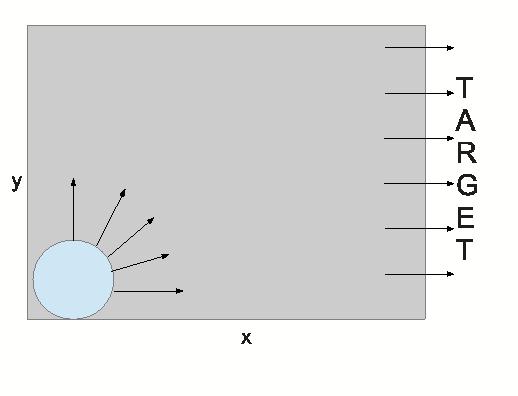
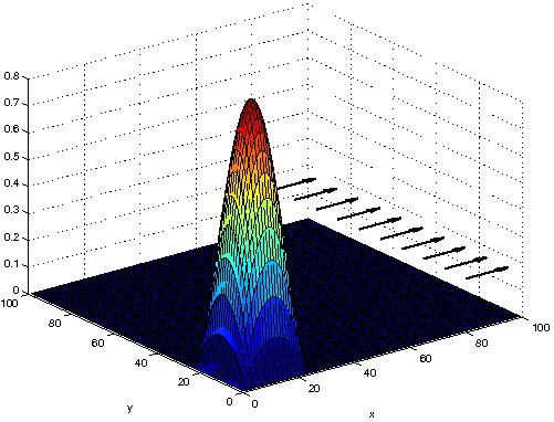
Let us first consider a group of individuals initially located near the corner of a rectangular room represented by the domain Ω=[0,1]×[0,1]⊆𝐑2\Omega=[0,1]\times[0,1]\subseteq{{\mathbf{R}}}^{2}, as shown in Figure 3.

Let us suppose that all of them are moving, at time t=0t=0, with constant velocity vv but with five different directions given by θi=i​π/8\theta_{i}=i\pi/8, i=0,…,4i=0,\ldots,4. Moreover, the individuals are equally distributed among these directions. In that moment some panic situation occurs at that corner and all of them try to move towards the exit, which is indicated by the parallel arrows in Figure 3.
Refer to caption
Figure 3: Initial condition for case-study 1. A crowd localized in the bottom-left corner is constituted by individuals moving in five different directions, indicated by the arrows. The parallel arrows on the right show the exit of the room.

Notice that those individuals who are moving in the direction θ0=0\theta_{0}=0 are the most favored, as they are already moving towards the exit. However, we assume that the other individuals start to change their directions according to a table of games considering only the sensitivity to reach the target. Assuming that the activity is homogeneously distributed, i.e. u0u_{0} is constant, that Λ⁡(𝐱)=𝐱\Lambda({\mathbf{x}})={\mathbf{x}}, and taking v=0.03v=0.03 and α1=α2=α=0.06\alpha_{1}=\alpha_{2}=\alpha=0.06 we perform some simulations, obtaining the results shown in Figure 4.

We can observe that as time evolves the pedestrians are closer to the exit, because many of them were able to change their directions. It is worth mentioning that the fact of considering only the tendency to reach the target let the individuals correct their movements without getting confused by the tendency to follow the stream.
Refer to caption Refer to caption
(a) (b)
Refer to caption Refer to caption
(c) (d)
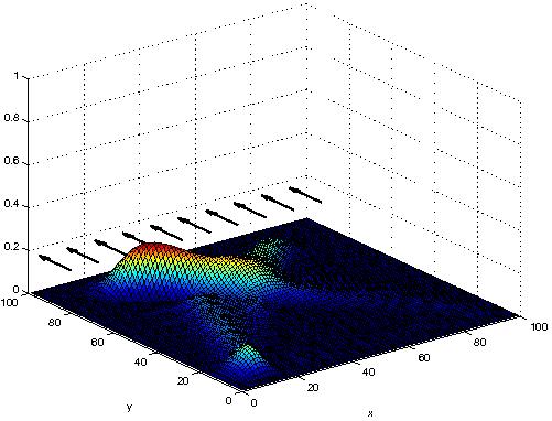
Figure 4: Case-study 1. Evolution of the density of the crowd for different times. (a) corresponds to the initial density, while (b)-(d) show its evolution. The parallel arrows indicate the target.

In Figure 5 we show a top view comparing the cases α=0\alpha=0 and α=0.06\alpha=0.06 for a fixed time. It becomes clear that originally the five groups were following different targets and that the model is successful predicting the reaction after a panic situation.

Refer to caption Refer to caption
(a) (b)
Figure 5: Case-study 1. Comparison between the evolution for (a) α=0\alpha=0 and (b) α=0.06\alpha=0.06.

Case-study 2

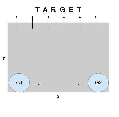
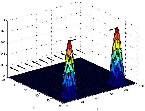
Let us consider two different groups, labeled by G​1G1 and G​2G2, which are initially moving towards two different targets inside the rectangular room, as shown in Figure 6. Both groups have the same velocity modulus vv and we consider five directions of movement θi=i​π/4\theta_{i}=i\pi/4, i=0,…,4i=0,\ldots,4. In this way, G​1G1 and G​2G2 are initially moving in the directions θ0=0\theta_{0}=0 and θ4=π\theta_{4}=\pi, respectively.

Refer to caption
Figure 6: Initial condition for case-study 2. Two crowds originally moving in opposite directions, indicated by the arrows. The parallel arrows in the top show the exit of the room.

Once more, we assume that they realize about the location of the exit, which corresponds to the direction θ2=π/2\theta_{2}=\pi/2, and they consequently try to adapt their movement. Notice that in this case none of the groups originally have the proper direction of movement.

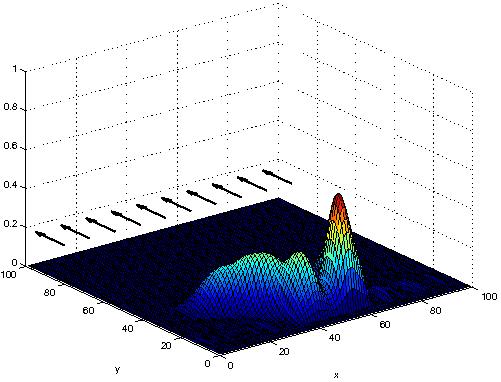
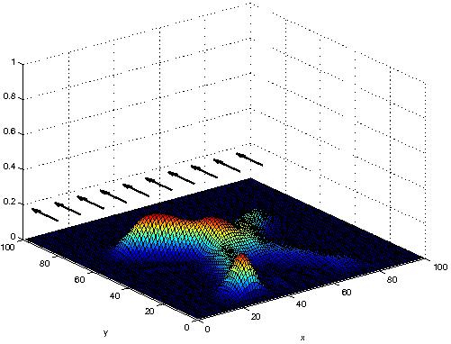
The table of games takes into account that the individuals can change their direction with a certain probability in order to reach the exit. However, we consider that individuals from group G​1G1 have better abilities, changing their direction with a probability α1=0.2\alpha_{1}=0.2, while individuals from group G​2G2 do it with a probability α2=0.1\alpha_{2}=0.1. The simulations are performed with these values and taking Λ⁡(𝐱)=𝐱\Lambda({\mathbf{x}})={\mathbf{x}} and v=0.03v=0.03. The results are shown in Figure 7.

Refer to caption Refer to caption
(a) (b)
Refer to caption Refer to caption
(c) (d)
Figure 7: Case-study 2. Evolution of the density of the crowds for different times. (a) corresponds to the initial density and the arrows on each crowd indicate the initial direction, while (b)-(d) show the evolution. The parallel arrows indicate the target.

In Figure 8 we show a top view comparing the afore-said situation with the case in which α1=α2=0.2\alpha_{1}=\alpha_{2}=0.2. Notice about the asymmetric shape of the crowd in Figure 8(a), clearly given by the different abilities (e.g. visual, fitness) that each group exhibits.

Refer to caption Refer to caption
(a) (b)
Figure 8: Case-study 2. Comparison between the evolution for (a) α1=0.2\alpha_{1}=0.2, α2=0.1\alpha_{2}=0.1 and (b) α1=α2=0.2\alpha_{1}=\alpha_{2}=0.2.

7 Looking Ahead to Perspectives

Various approaches to modeling crowd dynamics corresponding to different representation scales and related mathematical tools have been reviewed and critically analyzed in the survey paper [6]. The mesoscopic approach in this present paper has been selected, out of this overall analysis, as the most appropriate, according to the authors’ bias, to capture the complexity features of the system under consideration. Moreover, the use of discrete velocity variables has been adopted to model the micro-scale state of pedestrians in order to capture the granular features of their dynamics [13].

The use of discrete velocity variables was introduced, as already mentioned, to model vehicular traffic[15, 12], while the approach was further developed toward crowd modeling in [3]. The discretization is here applied to the velocity variable. In principles, it can be referred also to the space variable as already known for models of vehicle dynamics [16]. However, the technical difficulty of dealing with more than one space variables creates nontrivial technical problems, which do not seem yet solved at present.

The modeling approach proposed in this paper refers to normal flow conditions, namely when pedestrians are sufficiently relaxed to behave normally. On the other hand, the behavioral influence of panic conditions can play an important role in the modification of the usual dynamics [19, 20]. This objective can be pursued by an appropriate tuning of the model proposed in this paper also by taking advantage of recent studies on the behavioral dynamics of pedestrians [25, 27], and evolutive game theory [11]. Accordingly, the guidelines toward this important objective are given:

  • •

    Pedestrians undergo a trend to higher values of the activity variable. Moreover, the dynamics over the said variable has to be necessarily inserted in the model;

  • •

    The effective visibility zone becomes larger and signals from large distance become important, while in the case of normal conditions short distance signals appear to be more important;

  • •

    Pedestrians appear to be sensitive to crowd concentration, while in normal conditions they attempt to avoid it. Therefore different weights ε\varepsilon need to be used;

  • •

    The role of boundary conditions needs to be properly modeled arguably by means of nonlocal conditions

Moreover an important topic to be studied is the role of control actions by external systems. Namely the system needs to be modeled as an open one.

References

  • [1] G. Ajmone Marsan, N. Bellomo and M. Egidi, Towards a mathematical theory of complex socio-economical systems by functional subsystems representation, Kinetic Related Models, 1 (2008), 249–278.
  • [2] C. Appert-Rolland, P. Degond, and S. Motsch, Two-way multi-lane traffic model for pedestrians in corridors, Netw. Heterog. Media, 6 (2011), 351–381.
  • [3] N. Bellomo and A. Bellouquid, On the modeling of crowd dynamics: Looking at the beautiful shapes of swarms, Netw. Heterog. Media, 6 (2011), 383–399.
  • [4] N. Bellomo and A. Bellouquid, Global solution to the Cauchy problem for discrete velocity models of vehicular traffic, J. Differ. Equations, 252 (2012), 1350–1368.
  • [5] N. Bellomo and C. Dogbè, On the modelling of traffic and crowds - a survey of models, speculations, and perspectives, SIAM Rev., 53 (2011), 409–463.
  • [6] N. Bellomo, B. Piccoli and A. Tosin, Modeling crowd dynamics from a complex system viewpoint, Math. Models Methods Appl. Sci., 22 (2012) 1230004, (29 pages).
  • [7] N. Bellomo and J. Soler, On the mathematical theory of the dynamics of swarms viewed as complex systems, Math. Models Methods Appl. Sci., 22 (2012) 1140006, (29 pages).
  • [8] A. Bellouquid, E. De Angelis and L. Fermo, Towards the modeling of vehicular traffic as a complex system: a kinetic theory approach, Math. Models Methods Appl. Sci., 22 (2012) 1140003, (35 pages).
  • [9] S. Buchmuller and U. Weidman, Parameters of pedestrians, pedestrian traffic and walking facilities, ETH Report Nr. 132 (2006).
  • [10] V. Coscia and C. Canavesio, First-order macroscopic modelling of human crowd dynamics, Math. Models Methods Appl. Sci., 18 (2008), 1217–1247.
  • [11] V. Coscia, L. Fermo and N. Bellomo, On the mathematical theory of living systems II: The interplay between mathematics and system biology, Comput. Math. Appl., 62 (2011), 3902–3911.
  • [12] V. Coscia, M. Delitala and P. Frasca. On the mathematical theory of vehicular traffic flow II. Discrete velocity kinetic models. Int. J. Nonlinear Mech., 42 (2007), 411–421.
  • [13] E. Cristiani, B. Piccoli and A. Tosin, Multiscale modeling of granular flows with application to crowd dynamics, Multiscale Model. Sim., 9 (2011), 155–182.
  • [14] C. F. Daganzo, Requiem for second-order fluid approximation of traffic flow, Transport. Res. B-Meth., 29B (1995), 277–286.
  • [15] M. Delitala and A. Tosin, Mathematical modeling of vehicular traffic: a discrete kinetic theory approach, Math. Models Methods Appl. Sci., 17 (2007), 901–932.
  • [16] L. Fermo and A. Tosin, A fully-discrete-state kinetic theory approach to modeling vehicular traffic, arXiv:1210.7988, (2012)
  • [17] L. Gosse, Computing qualitatively correct approximations of balance laws, SIMAI Springer Series, Vol. 2, (2013).
  • [18] D. Helbing, A mathematical model for the behavior of pedestrians, Behav. Sci., 36 (1991), 298–310.
  • [19] D. Helbing, I. Farkas and T. Vicsek. Simulating dynamical feature of escape panic, Nature, 407 (2000), 487–490.
  • [20] D. Helbing, A. Johansson and H. Z. Al-Abideen, Dynamics of crowd disasters: An empirical study, Phys. Rev. E, 75 (2007), 046109.
  • [21] D. Helbing and M. Moussaid, Analytical calculation of critical perturbation amplitudes and critical densities by non-linear stability analysis for a simple traffic flow model, Eur. Phys. J. B, 69 (2009), 571–581.
  • [22] H. Holden, K. Karlsen, K. Lie and N. Risebro, Splitting methods for partial differential equations with rough solutions, EMS Series of Lectures in Mathematics, Analysis and MATLAB programs, European Mathematical Society (EMS), Zürich, (2010).
  • [23] D. Knopoff, On the modeling of migration phenomena on small networks, Math. Models Methods Appl. Sci., 23 (2013), to appear.
  • [24] B. Maury, A. Roudneff-Chupin and F. Stantambrogio, A macroscopic crowd motion modelof gradient flow type, Math. Models Methods Appl. Sci., 20 (2010), 1899–1940.
  • [25] M. Moussaïd, D. Helbing, S. Garnier, A. Johansson, M. Combe, and G. Theraulaz, Experimental study of the behavioural mechanisms underlying self-organization in human crowds, Proc. Roy. Soc. B, 276 (2009), 2755–2762.
  • [26] B. Piccoli and A. Tosin, Time-evolving measures and macroscopic modeling of pedestrian flow, Arch. Ration. Mech. An., 199 (2011), 707–738.
  • [27] D. Roggen, M. Wirz, G. Tröster and D. Helbing, Recognition of crowd behavior from mobile sensors with pattern analysis and graph clustering methods, Netw. Heterog. Media, 6 (2011), 521–544.
  • [28] F. C. Santos, J. M. Pacheco and T. Lenaerts, Evolutionary dynamics of social dilemmas in structured heterogeneous populations, P. Natl. Acad. Sci. USA, 103 (2006), 3490–3494.
  • [29] F. C. Santos, V. Vasconcelos, M. D. Santos, P. Neves and J. M. Pacheco, Evolutionary dynamics of climate change under collective-risk dilemmas, Math. Models Methods Appl. Sci., 22 (2012) 1140004, (17 pages).
  • [30] A. Schadschneider and A. Seyfried, Empirical results for pedestrian dynamics and their implications for modeling, Netw. Heterog. Media, 6 (2011), 545–560.
  • [31] Y. Yazici, Operator splitting methods for differential equations, Ph.D. Thesis at Izmir Institute of Technology, (2010).