Inferring the nature of the boson at 125-126 GeV
Abstract
The presence of a bosonic resonance near 125 has been firmly established at the Large Hadron Collider. Understanding the exact nature of this boson is a priority. The task now is to verify whether the boson is indeed the scalar Higgs as proposed in the Standard Model of particle physics, or something more esoteric as proposed in the plethora of extensions to the Standard Model. This requires a verification that the boson is a state with couplings precisely as predicted by the Standard Model. Since a non Standard Model boson can in some cases mimic the Standard Model Higgs in its couplings to gauge bosons, it is essential to rule out any anomalous behavior in its gauge couplings. We present a step by step methodology to determine the properties of this resonance without making any assumptions about its couplings. We present the analysis in terms of uni-angular distributions which lead to angular asymmetries that allow for the extraction of the couplings of the 125-126 resonance to Z bosons. We show analytically and numerically, that these asymmetries can unambiguously confirm whether the new boson is indeed the Standard Model Higgs boson.
pacs
12.60.-i, 14.80.Bn, 14.80.EcI Introduction
A new bosonic resonance with a mass of about 125 has recently been observed at the Large Hadron Collider by both ATLAS Collaboration [1, 2] and CMS Collaboration [3, 4, 5]. The mass of the resonance is suggestive that this resonance is the Higgs boson that should exist in the Standard Model of particle physics as a spin zero parity-even resonance. Significant effort is now directed at determining the properties and couplings of this new resonance to confirm that it is indeed the Higgs boson of the Standard Model. In this work we specify this new boson by the symbol and we call it the Higgs, even though it has not been proved to be the Higgs of the Standard Model. This resonance is observed primarily in three decay channels , and , where one (or both) of the ’s and ’s are off-shell. It is well known that the spin and parity of the resonance and its couplings can be determined by studying the momentum and angular distributions of the decay products. Indeed there is little doubt that a detailed numerical fit to the invariant masses of decay products and their angular distributions will reveal the true nature of this resonance. However, a detailed study of the angular distributions requires large statistics and may not be feasible currently. Several studies existed in the literature before the discovery of this new resonance [6, 7, 8, 9, 10, 11, 12, 13, 14, 15, 16, 17, 18, 19, 20, 21, 22, 23, 24, 25, 26, 27, 28, 29, 30, 31, 32, 33, 34, 35, 36] and yet several papers have appeared recently on strategies to determine the spin and parity of the resonance [38, 37, 39, 40, 41, 42, 43, 44, 45, 46, 47, 48, 49, 50]. Yet, there is no clear conclusion on the step by step methodology to determine these properties and convincingly establish that the new resonance is indeed the Standard Model Higgs boson. The recent result [5] from CMS Collaboration on the determination of spin and parity of the new boson is not conclusive.
In this paper we are exclusively concerned with Higgs decaying to four charged leptons, which proceeds via a pair of bosons: where , are leptons or . Since the Higgs is not heavy enough to produce two real bosons, we can have one real and another off-shell , or both the ’s can be off-shell. While we deal with the former case in detail our analysis applies equally well to the later case. We find that only in a very special case dealing with boson it is more likely that both the bosons are off-shell. We emphasize that the final state is not equivalent to or as sometimes mentioned in the literature, since the latter final states have to be anti-symmetrized with respect to each of the two sets of identical fermions in the final state. The anti-symmetrization of the amplitudes is not done in our analysis and hence our analysis applies only to . We examine the angular distributions and present a strategy to determine the spin and parity of , as well as its couplings to the -bosons with the least possible measurements. Since the decay mode has been observed, is necessarily a boson and the Landau-Yang theorem [51, 52] excludes that it has spin . Further, assuming charge conjugation invariance, the observation of also implies [10] that is a charge conjugation state. In making this assignment of charge conjugation it is assumed that is an eigenstate of charge conjugation. With the charge conjugation of thus established we will only deal with the parity of henceforth. We consider only Spin-0 and Spin-2 possibilities for the boson. Higher spin possibilities need not be considered for a comparative study as the number of independent helicity amplitudes does not increase any more [53, 15]. The process under consideration requires that Bose symmetry be obeyed with respect to exchange of the pair of bosons. This constraints the number of independent helicity amplitudes to be less than or equal to six. Even if the Spin- of is higher (i.e. ), the number of independent helicity amplitudes still remains six. However, the helicity amplitudes corresponding to higher spin states involve higher powers of momentum of , independent of the momentum dependence of the form factors describing the process. We will show that even for under a special case only two independent helicity amplitudes may survive just as in the case of . The two cases are in principle indistinguishable unless one makes an assumption on the momentum dependence of the form factors involved.
We start by considering the most general decay vertex for both scalar and tensor resonances decaying to two bosons. We evaluate the partial decay rate of in terms of the invariant mass squared of the dilepton produced from the non-resonant and the angular distributions of the four lepton final state. We demonstrate that by studying three uni-angular distributions one can almost completely determine the spin and parity of and also explore any anomalous couplings in the most general fashion. We find that and can easily be excluded. The and possibilities can also be easily distinguished, but may require some lepton invariant mass measurements if the most general tensor vertex is considered. Only if is found to be of Spin-2, a complete three angle fit to the distribution is required to distinguish between and .
The determination of couplings and spin, parity of the boson is important as there are other Spin-0 and Spin-2 particles predicted, such as the radion [56, 55, 57, 58, 59, 60, 61] and Kaluza-Klein graviton [62, 63, 64, 45], which can easily mimic the initial signatures observed so far. Such cases have already been considered in the literature even in the context of this resonance. Our analysis is most general and such extensions are limiting cases in our analysis as the couplings are defined by the model.
In Section II we layout the details of our analysis, with Sections II.1 and II.2 devoted exclusively to Spin-0 Higgs and Spin-2 boson respectively. A step by step comparison with detailed procedure to distinguish the spin and parity states of the new boson is discussed in Sec. II.3. In Sec.II.4 we present a numerical study to demonstrate the discriminating power of the uni-angular distribution analysis compared to the current approach [65, 66]. We find that uni-angular distribution is more powerful in discriminating between the scalar () and pseudoscalar () hypothesis.
We conclude emphasizing the advantage of our approach in Section III.

II Decay of the new resonance to four charged leptons via two bosons
Let us consider the decay of to four charged leptons via a pair of bosons:
where , are leptons or . As mentioned in the introduction we assume and are not identical. The kinematics for the decay is as shown in Fig. 1. The Higgs at rest is considered to decay with the on-shell moving along the axis and off-shell along the axis. The decays of and are considered in their rest frame. The angles and momenta involved are as described in Fig. 1. The 4-momenta of , and are defined as , and respectively. We choose to decay to lepton pair with momentum and respectively and to decay to with momentum and respectively.
Nelson [6, 7, 8] and Dell’Aquilla [7] realized the significance of studying angular correlations in this process with Higgs boson decaying to a pair of bosons for inferring the nature of the Higgs boson. Refs. [12, 14, 15] were the first to extend the analysis to include higher spin possibilities so that any higher spin particle can effectively be distinguished from SM Higgs. We study similar angular correlations in this paper. We begin the study by considering the most general vertices for a and a resonance . We shall first discuss the two spin possibilities separately. Later we will layout the approach to distinguish them assuming the most general vertex.
II.1 Spin-0 Higgs
The most general vertex factor for Spin-0 Higgs is given by
| (1) |
where is the weak mixing angle, is the electroweak coupling, and , , are some arbitrary form factors dependent on the 4-momentum squares specifying the vertex. The vertex is derived from an effective Lagrangian (see for example Ref. [54]) where higher dimensional operators contribute to the momentum dependence of the form factors. Since the effective Lagrangian in the case of arbitrary new physics is not known, no momentum dependence of , and can be assumed if the generality of the approach has to be retained. Approaches using constant values for the form factors therefore cannot provide unambiguous determination of spin-parity of the new boson. We emphasize that even though the momentum dependence of , and is not explicitly specified, they must be regarded as being momentum dependent in general. In SM, however, , , are constants and take the value and at tree level.
In Eq. (1) the term proportional to is odd under parity and the terms proportional to both and are even under parity. Partial-wave analysis tells that such a decay gets contributions from the first three partial waves, namely -wave, -wave and -wave. Since - and -waves are parity even while the -wave is parity odd, the term associated with effectively describes the -wave contribution. The terms proportional to and are admixtures of - and -wave contributions. The decay of a Spin-0 particle to two Spin-1 massive particles is hence always described by three helicity amplitudes.
The decay under consideration is more conveniently described in terms of helicity amplitudes , and defined in the transversity basis as
| (2) | ||||
| (3) | ||||
| (4) |
where and are the invariant masses of the and lepton pairs, i.e. , ,
| (5) |
, and are the coefficients that enter the most general vertex we have written in Eq. (1) and
| (6) |
It should be remembered that the helicities and are in general functions of and , even though the functional dependence is not explicitly stated. The advantage of using the helicity amplitudes is that the helicity amplitudes are orthogonal. Our helicity amplitudes are defined in the transversity basis and thus differ from those given in Ref. [54]. Our amplitudes can be classified by their parity: and are parity even and is parity odd. This is unlike the amplitudes used in Ref. [54]. Throughout the paper we use linear combinations of the helicity amplitudes such that they have well defined parity. This basis may be referred to as the transversity basis. Even though we work in terms of helicity amplitudes in the transversity basis, we will show below, it is in fact possible to uniquely extract out the coefficients which characterize the most general vertex for Higgs.
We will assume that is on-shell while is off-shell, unless it is explicitly stated that both the bosons are off-shell. The off-shell nature of the is denoted by a superscript ‘*’. One can easily integrate over using the narrow width approximation of the . The helicity amplitudes are then defined at and . In principle could also have been explicitly integrated out in both the cases when either is off-shell or fully on-shell, resulting in some weighted averaged value of the helicities. The differential decay rate for the process , after integrating over (assuming is on-shell or even otherwise) can now be written in terms of the angular distribution using the vertex given in Eq. (1) as:
| (7) |
where the helicity fractions , and are defined as
| (8) |
where and
| (9) | ||||
| (10) |
where is the total decay width of the boson, is the branching ratio for the decay of boson to two mass-less leptons: and we have used the narrow width approximation for the on-shell . We emphasize that with integrated out the helicity amplitudes and helicity fractions are functions only of . In Eq. (7) is defined as
| (11) |
with and , and is the 2nd degree Legendre polynomial:
| (12) |
We have chosen to express the the differential decay rate in terms of Legendre polynomials for and and Fourier series for . This ensures that each term in Eq. (7) is orthogonal to any other term in the distribution. The Legendre polynomials and satisfy the orthogonality condition since the range of and is to , whereas that of is to . Our approach of using Legendre polynomials and the choice of helicity amplitudes in transversity basis classified by parity form the corner-stone of our analysis. The same technique will be used in Sec. II.2 to analyze the Spin-2 case.
An interesting observation in the scalar case is that the coefficients of and are identically equal to in both magnitude and sign. It is worth noting that the coefficients of and are also identically equal to in both magnitude and sign.
Integrating Eq. (7) with respect to or or , the following uni-angular distributions are obtained:
| (13) | ||||
| (14) | ||||
| (15) |
where
| (16) | ||||
| (17) | ||||
| (18) | ||||
| (19) | ||||
| (20) | ||||
| (21) |
are explicitly functions of . The superscript indicates the spin of . Since , , , , , and are orthogonal functions, the coefficients of each of the terms can be extracted individually. We can also extract all the above coefficients in terms of asymmetries defined as below:
| (22) | ||||
| (23) | ||||
| (24) | ||||
| (25) | ||||
| (26) | ||||
| (27) |
As had already been realized from Eq. (7), the coefficients of and as well as the coefficients of and in Eqs. (13) and (14) are identical. This results in a maximum of 6 possible independent measurements , , , , and using uni-angular analysis. For the decay under consideration, and . Substituting the experimental value for the weak mixing angle: , we get and . Owing to such small values of and it is unlikely that , and can be measured using the small data sample current available at LHC, reducing the number of independent measurable to three.
Using Eqs. (16) and (17) and the identity , the following solutions for , and are obtained:
| (28) | ||||
| (29) | ||||
| (30) |


We have shown that one can easily measure all the three helicity fractions using uni-angular distributions. We can also measure , which is proportional to sine of the phase difference between the two helicity amplitudes and . In other words, we can also measure the relative phase between the parity-odd and parity-even amplitudes. Such a phase can arise if -symmetry is violated in interactions or could indicate pseudo-time reversal violation arising from loop level contributions or rescattering effects akin to the strong phase in strong interactions. Since such a term requires contributions from both parity-even and parity-odd partial waves, in SM. In the case of SM we have and . Assuming narrow width approximation for the on-shell we get
| (31) | ||||
| (32) |
Clearly, for the case of SM the term has a characteristic dependence on . Demanding , we get
| (33) |
and
| (34) |
Thus for SM we can predict the experimental values for the coefficients and as:
| (35) |
It is evident that and are functions of alone and are uniquely predicted in the SM. and are pure numbers for a given value of . Their variation with respect to is shown in Fig. 2a. It is clear from the plot that is always negative while is always positive in the SM. The variation of the helicity fractions with respect to is shown in Fig. 2b. Fig. 2c also shows the variation of the normalized differential decay width of the SM Higgs decaying to four charged leptons via two bosons, with respect to . Fig. 2 contains all the vital experimental signatures of the SM Higgs and must be verified in order for the new boson to be consistent with the SM Higgs boson. We emphasize that a nonzero measurement of will be a litmus test indicating a non-SM behavior for the Higgs. Furthermore, a non-zero would imply that the observed resonance is not of definite parity.
If we find the new boson to be of , but still not exactly like the SM Higgs, then we need to know the values of and in the vertex factor of Eq. (1). It is easy to find that for a general boson, the values of both and are given by
| (36) | ||||
| (37) |
For SM and at tree level only. At loop level even within SM these values would differ. It may be hoped that and determined in this way may enable testing SM even at one loop level once sufficient data is acquired. This is significant as triple-Higgs vertex contributes at one loop level and measurement of may provide the first verification of the Higgs-self coupling. Even if the scalar boson is not a parity eigenstate but an admixture of even and odd parity states, Eqs. (36) and (37) can be used to determine and . We can determine by measuring :
| (38) |
Therefore, it is possible to get exact solutions for in terms of the experimentally observable quantities like , , and .
We want to stress that it is impossible to extract out both and by measuring only one uni-angular distribution (corresponding to either or ), since the helicity amplitude contains both and . Hence, it is not possible to conclude that the boson is a Standard Model Higgs by studying or distributions alone.
The current data set is limited and may allow binning only in one variable. We therefore examine what conclusions can be made if is also integrated out and only the three uni-angular distributions are studied individually. As can be seen from Eqs. (36), (37) and (38) we can obtain some weighted averages of and . These equations will only allow us to verify whether and . In addition the presence of any phase between the parity-even and parity-odd amplitudes can still be inferred from Eq. (18). The integrated values for the observables and are uniquely predicted in SM at tree level to be and respectively.
II.2 Spin-2 Boson
As stated in the Introduction we shall use the same symbol to denote the boson even if it is of Spin-2. The most general vertex factor for Spin-2 boson, with polarization has the following tensor structure
| (39) | |||||
where and are the polarizations of the two bosons; , , , , and are arbitrary coefficients and is the difference of the four momenta of the two ’s, i.e. . Only the term that is associated with the coefficient is dimensionless. The form of the vertex factor ensures that and , which stem from the fact that the field of a Spin-2 particle is described by a symmetric, traceless tensor with null four-divergence. Here like the Spin-0 case is the sum of the four-momenta of the two ’s, i.e. . Since we are considering the decay of Higgs to two bosons, the vertex factor must be symmetric under exchange of the two identical bosons. This is taken care of by making the vertex factor symmetric under simultaneous exchange of and corresponding momenta of and . The Lagrangian that gives rise to the vertex factor contains higher dimensional operators, which are responsible for the momentum dependence of the form factors.
In the terms that are proportional to and are parity-odd and the rest of the terms in are parity-even. From helicity analysis it is known that the decay of a massive Spin-2 particle to two identical, massive, Spin-1 particles is described by six helicity amplitudes. Bose symmetry between the pair of Z bosons [67, 68] imposes constraints on the vertex such that it gets contributions from two parity-odd terms that are admixture of one -wave and one -wave, and four parity-even terms that are some combinations of one -wave, two -waves and one -wave contributions. Even for the case of Spin-2 boson we choose to work with helicity amplitudes as they are orthogonal but choose a basis such that amplitudes have definite parity associated with them. We find the following six helicity amplitudes in transversity basis:
| (40) | ||||
| (41) | ||||
| (42) | ||||
| (43) | ||||
| (44) | ||||
| (45) |
where , , and are defined as
| (46) | ||||
| (47) | ||||
| (48) | ||||
| (49) |
The quantity is as defined in Eq. (5).
We wish to clarify that our vertex factor is the most general one. An astute reader can easily write down terms that are not included in our vertex and wonder how such a conclusion of generality can be made. For example, one can add a new possible term such as . It is easy to verify that this new form factor enters our helicity amplitudes and in the combination :
| (50) | ||||
| (51) |
Note that only this combination of and is accessible to experiments and all other helicity amplitudes remain unchanged. Since, there exist only six independent helicity amplitudes corresponding to six partial waves for the Spin-2 case, the number of helicity amplitudes in the transversity basis must also be six. Adding any new terms to the vertex factor will simply modify the expressions for the helicity amplitudes. The generality of our vertex is therefore very robust. Having established the generality of we will henceforth not consider any term absent in the vertex of Eq. (39). Our helicity amplitudes are different from those given in Ref. [54]. In Ref. [54], they provide eight independent helicity amplitudes. If we consider the Bose symmetry of the two identical vector bosons to which is decaying, then these should reduce to six independent helicity amplitudes. Again as stated in the scalar case, our helicity amplitudes are classified by their parity and thus differ from those in Ref. [54]. Our amplitudes and have parity-odd behavior, and the rest of the helicity amplitudes have parity-even behavior. In contrast not all the amplitudes enunciated in Ref. [54] have clear parity characteristics.
Once again just as in the scalar case we will start by assuming that is on-shell while is off-shell. The integration over is done using the narrow width approximation of the . In tensor case, however, off-shell will also have to be considered in a special case. We hence consider that is explicitly integrated out whether is off-shell or fully on-shell. In case is off-shell the resulting helicities are some weighted averaged value and should not be confused with well defined values at . The differential decay rate for the process , after integrating over (assuming is on-shell or even otherwise) can now be written in terms of the angular distribution using the vertex given in Eq. (39) as:
| (52) |
where includes all the terms that are proportional to and written explicitly in the appendix, Eq. (92). The helicity fractions are defined as
| (53) |
and is given by
| (54) |
where and we have averaged over the 5 initial polarization states of the spin-2 boson.
The uni-angular distributions are given by
| (55) | ||||
| (56) | ||||
| (57) |
where the superscript is used to denote the fact that the concerned coefficients are for spin-2 resonance, and
| (58) | ||||
| (59) | ||||
| (60) | ||||
| (61) | ||||
| (62) | ||||
| (63) | ||||
| (64) | ||||
| (65) |
These coefficients can again be extracted from asymmetries similar to those defined in Eqs. (22), (23), (24), (25), (26) and (27) for the spin-0 case. We find that the angular distributions corresponding to and are different in the Spin-2 case in contrast to the Spin-0 case. This feature can enable us to distinguish between the two spins, unless the difference happens to be zero for certain choice of parameters, even in the Spin-2 case. Considering only the independent terms in Eqs. (55) and (56), the difference between the coefficients of and in and respectively, is
| (66) |
If we find that for all , then the tensor case would have similar characteristics in the uni-angular distributions as discussed in the scalar case. However, this can only happen if helicity amplitudes (or equivalently the corresponding coefficients , , , , and ) have the explicit momentum dependence so as to absorb completely in . The reader can examine the expression for to conclude that this is impossible and the only way can be equated to zero for all , is when
| (67) |
In such a special case all the form-factors in vertex vanish, except and . This special case explicitly implies that the parity of the Spin-2 boson is even. We will refer to this case as the special case, since the uni-angular distribution mimics the case. Working under this special case
| (68) | ||||
| (69) | ||||
| (70) |
where the , and are now given by
| (71) | ||||
| (72) | ||||
| (73) |
Now using the identity , we get
| (74) |
Note the similarity between Eqs. (33) and (74). The conclusions that when can also be drawn if integrated over and is found to be non zero. However, it clear from Eq. (66) that the domain of integration for and cannot be symmetric.

II.3 Comparison Between Spin-0 and Spin-2
Having discussed both the scalar and tensor case, we summarize the procedure to distinguish the spin and parity states of the new boson in a flowchart in Fig. 3. The procedure entailed, ensures that we convincingly determine the spin and parity of the boson. The first step should be to compare the uni-angular distributions in and . If the distribution is found to be different the boson cannot be the SM Higgs and indeed must have Spin-2. However, if the distributions are found to be identical the resonance can have Spin-0 or be a very special case of Spin-2 arising only from and terms in the vertex in Eq. (39). The similarity between Eqs. (33) and (74) makes it impossible to distinguish these two cases by looking at angular distributions alone.
The special case can nevertheless still be identified by examining the surviving helicity amplitudes and . The helicity amplitudes given in Eqs. (42) and (43) reduce in this special case to,
| (75) | ||||
| (76) |
These may be compared with Eqs. (2) and (3) to notice that they have identical form, except for an additional dependence in and expressions above. The additional dependence increases the contribution from both off-shell ’s (called ) significantly in comparison to the dominant one on-shell and one off-shell (called ) contribution expected in SM. In the SM one would expect the ratio of the number of events in to channel to be about . However, in the special case we would expect this ratio to be about . Thef reader is cautioned not to confuse this explicit dependence with any assumption on the momentum dependence of the form-factors. Throughout the analysis we have assumed the most general form-factors , , , , , , , and , nevertheless and turn out to have additional dependence in comparison to and respectively. This explicit dependence arises due to contributions only from higher dimensional operators in the special case.
Having excluded the Spin-2 possibility, the resonance would be a parity-odd state () if and a parity-even state () if . If the resonance is found to be in state, we need to check whether and terms are as predicted in SM. The values of and as a function of are plotted in Fig. 2. The integrated values for the observables and are uniquely predicted in SM at tree level to be and respectively. These tests would ascertain whether the state is the SM Higgs or some non-SM boson. If it turns out to be a non-SM boson, we can also measure the coefficients by using Eqs. (36), (37) and (38).
Finally we emphasize that our approach is unique in using helicity amplitudes in the transversity basis so that the amplitudes are classified by parity. We also use orthogonality of Legendre polynomials in and as well as a Fourier series in to unambiguously determine the spin and parity of the new resonance. Another significant achievement is the use of the most general vertex factors for both Spin-0 and Spin-2 cases allowing us to determine the nature of be it in any extension of the SM. We wish to stress that we consider neither any specific mode of production of the new resonance (like gluon-gluon fusion or vector boson fusion), nor any specific model for its couplings. The production channel for the new resonance has no role in our analysis. We consider its decay only to four leptons via two bosons. Most discussions in current literature deal either with specific production channels or with specific models of new physics which restrict the couplings to specific cases both for Spin-0 and Spin-2. Refs. [34, 38, 37, 46, 45] deal with graviton-like Spin-2 particles, while Ref. [47] deals with Spin-2 states that are singlet or triplet under . Ref. [34] considers polar angle distribution of and angular correlations between the charged leptons coming from decays to differentiate the Spin-0 and Spin-2 possibilities. While Ref. [37] looks at ‘Higgs’-strahlung process to distinguish the various spin and parity possibilities, Ref. [38] compares branching ratios of the new boson decaying to , and channels as a method to measure the spin and parity of the new boson. In Ref. [45] the authors propose a new observable that can distinguish SM Higgs from a Spin-2 possibility. They consider the three-body decay of the new resonance to a SM vector boson and a fermion-antifermion pair. Ref. [46] shows that the current data disfavors a particular type of graviton-like Spin-2 particle that appears in scenarios with a warped extra dimension of the AdS type. Refs. [47, 48] deal with Spin-0 or Spin-2 particles produced via vector boson fusion process alone. Our discussion subsumes all of the above special cases. Moreover, unlike other discussions in the literature we provide clearly laid out steps to measure the couplings, spin and parity of the new resonance without any ambiguity. We want to reiterate that it is important to measure not only the spin and parity of the new resonance but also its couplings before any conclusive statements can be made that it is the SM Higgs.
II.4 Numerical study of the uni-angular distributions
In this sub-section we study the possibility of using the uni-angular distributions, given in previous sub-section to differentiate the different possible spin states. For simplicity throughout this sub-section we will neglect the dependence of and . The signal and background events were generated using the MadEvent5 [69] event generator interfaced with PYTHIA 6.4 [70] and PGS 4 [71]. The vertex of Eq. (1) was implemented into the UFO format of Madgraph5 using Feynrules 1.6.18 [72]. Unlike the earlier sub-sections we also include the and final states because the identification of being the mother particle of the pair of same flavor opposite sign leptons with an invariant mass closest to the breaks the exchange symmetry of these final states in most regions of phase space. As the analysis of this paper has to do purely with the shape of the partial widths in the channel, the production mechanism is not crucial to understanding the spin and properties of the resonance at . However to be concrete, these samples were generated for collisions at using the CTEQ6L1 parton distribution functions (PDFs) [73]. We choose to follow the ATLAS cut based analysis of Ref. [74] instead of the CMS analysis [66] because the CMS analysis has used a more sophisticated multi-variate analysis (MVA) technique. We set the Higgs boson mass , which is close to what has been measured in Ref. [74]. The branching ratios and decay widths are set appropriately using the values from the Higgs working group webpage [75].
Following the analysis of Ref. [74] we impose the following lepton selection cuts and triggers. In particular, the single lepton trigger thresholds are for a muon(electron). The di-muon trigger thresholds used are for the symmetric case and and for the asymmetric case. For di-electrons the thresholds are . The lepton identification cuts require that each electron(muon) must have () with . Sorting leptons in decreasing order of , we also impose the selection criteria , and . For same flavor leptons we also require that while for opposite flavor . Furthermore we also impose the invariant mass cuts on the , and described in Table 1 to reduce the Standard Model background. is the invariant mass of the pair of opposite sign same flavor leptons closest to while is the other combination. The number of signal events in our simulation is in good agreement with the SM predicted value quoted in Ref. [74], while the background rate is slightly lower than total background rate because we have not included the sub-dominant processes like Z+jets and .
| Cuts | SM | |
|---|---|---|
| Selection | 22 | 1542 |
| GeV | 20 | 1432 |
| GeV | 19 | 1294 |
| GeV | 19 | 14 |
In order to quantify the effect of using the uni-angular distributions to extract the nature of the GeV resonance we construct the test statistic based on the ratio of the likelihoods
| (77) |
where the is the unbinned likelihood function
| (78) |
As our acceptances are in good agreement with the ATLAS predictions for the rest of our analysis we will assume a background rate events for luminosity due to the continuum background. However as the total observed number of events are slightly above the expected rate we need to marginalize over the expected signal rate. In particular we assume a bayesian prior flat distribution for . For a particular value of we generate ensembles of events to find the average of the product within the brackets in Eq. (78). The probability density function (PDF) for signal is the product of the distributions
| (79) | ||||
| (80) | ||||
| (81) |
where , and
| (82) | ||||
| (83) | ||||
| (84) | ||||
| (85) | ||||
| (86) |
while for the background . In the above approximations for we have neglected the dependences of and and integrated Eq (9), Eq. (13), Eq. (14) and Eq. (15) over . Furthermore we have performed a power law fit in term of for each of the coefficients. As and have dimensions of mass squared, in the above approximations for the different coefficients we have used the dimensionless coefficients and instead. By definition, the hypothesis corresponds to and the hypothesis corresponds to . When the magnitude of is not crucial as we normalize the and cross-sections so as to produce the same number of signal events.


To quantify power of the uni-angular distributions in hypothesis testing, we present the q test-statisic for the and hypotheses in Fig. 4. In particular, we have applied the q-statistic in Eq. (77) to samples of Monte Carlo events that have passed the above cuts in Tab. 1, where we assumed the above bayesian prior for the mean signal rate. The red (dark grey) curve corresponds to events while the green (light grey) curve corresponds to events. The solid curves correspond to a gaussian fit to these distributions and using them we define the separation power as
| (87) |
where is the area under the curve calculated from the point on the -axis which satisfies the condition that the area under the right tail of the left distribution is equal to the left tail of the right distribution and is the maximum of the two standard deviations.
The separation power using the q test statistic works well for low luminosity, but this approach loses sensitivity at larger luminosity. To illustrate this point we present Fig. 5 at a function of luminosity. The red (dark grey) points correspond calculated separation power for a particular luminosity while the green (light grey) curve is a fit to the data. The lowest data point corresponds to a luminosity of with an observation of 43 events while for at higher luminosities we have assumed that the number of observed events agrees with the expected rates. Furthermore this extrapolation assumes the same cuts and efficiencies for higher luminosities. For luminosities greater that , a fit of the uni-angular distributions would probably provide a stronger hypothesis test.
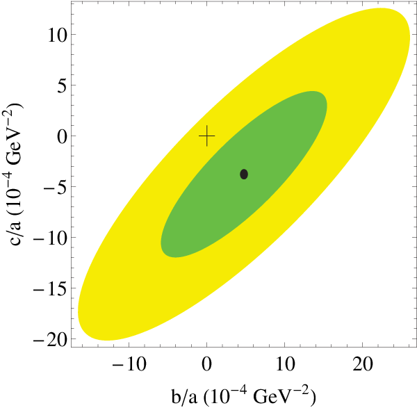
It would seem that the values of all the form factors , and can be extracted using the there uni-angular distributions Eq. (79)-(81) along with Eq. (82)-(86). However, the difference between the uni-angular distributions in Eq. (79) and Eq. (80) is small because it is proportional to . Given the small sample of 43 events this would essentially imply that only two parameters can be obtained. Our numerical work confirms this fact. Since , , , and are orthogonal functions the coefficients of each of the terms can be extracted individually. As discussed in Sec. II.1 this would result in four observables. We emphasize that as the data sample increases the additional information can be used to measure relative phases between , and . For 43 events, as expected from the discussions in Sec. II.1 based on the small value of in SM, we find we could only extract stable values of and by maximizing the likelihood function . One can also estimate the errors in and from the inverse of the covariance matrix defined as
| (88) |
where . Here denotes those values of the parameters that maximizes the likelihood function. In Fig. 6 we present the extract values of and for a sample of 43 events. Using these values of and , the value of can also be found by fitting the decay width in Eq. (82) to the Standard Model partial width. Using this approach, the values of , and with their respective errors are
| (89) | ||||
| (90) | ||||
| (91) |
III CONCLUSION
We conclude that by looking at the three uni-angular distributions and examining the numbers of to events one can unambiguously confirm whether the new boson is indeed the Higgs with and with couplings to bosons exactly as predicted in the Standard Model. We show that the terms in the angular distribution corresponding to and play a critical role in distinguishing the and states. The distributions are identical for Spin-0 case, but must be different for Spin-2 state except in a special case where . The ratio of the number of events to the number of events provides a unique identification for this special case. In this special case the number of events dominates significantly over the number of events. The Spin-2 resonance can thus be unambiguously confirmed or ruled out. With Spin-2 possibility ruled out, Spin-0 can be studied in detail.
The resonance would then be a parity-odd state () if and a parity-even state () if . If the resonance is found to be in state, we need to check whether and terms are as predicted in SM. The integrated values for the observables and are uniquely predicted in SM at tree level to be and respectively. These tests would ascertain whether the state is the SM Higgs or some non-SM boson. If it turns out to be a non-SM boson, we can also measure the coefficients by using Eqs. (36), (37) and (38). If the boson is a mixed parity state, the relative phase between the parity-even and parity-odd amplitudes can also be measured by studying the term in the uni-angular distribution. We present a step by step methodology in Fig. 3 for a quick and sure-footed determination of spin and parity of the newly discovered boson. Our approach of using Legendre polynomials and the choice of helicity amplitudes classified by parity enable us to construct angular asymmetries that unambiguously determine if the new resonance is indeed the Standard Model Higgs.
Numerically we have have simulated the dominant continuum background and Standard Model signal shown that our acceptances are in good agreement with the ATLAS predictions. Using the uni-angular distributions derived in this paper we compute the q-statistic . We observe the separation power of this approach is most powerful at low luminosity assuming that the cuts and the acceptances remain the same at each luminosity. For easy experimental adaption we have included power law parametrization of the various angular coefficients in terms of the fundamental Higgs vertex parameters. We also obtain fits for and for a 43-event sample, demonstrating that both and can be constrained by a rather small sample of data.
Acknowledgements.
RS is grateful to Institute of Physics, Academia Sinica, for hospitality where part of the work was done. We thank Sridhara Dasu for discussions. AM is supported by the U.S. Department of Energy under Contract No. DE-FG02-96ER40969.Appendix A Other Terms in the Angular Distributions
In the main text, we have not included the and dependent term in the angular distributions for the case of Spin-2 boson. However, for the sake of completeness, the and dependent term in the angular distributions are given below.
| (92) |
References
- [1] G. Aad et al. [ATLAS Collaboration], Phys. Lett. B 716, 1 (2012) [arXiv:1207.7214 [hep-ex]].
- [2] G. Aad et al. [ATLAS Collaboration], Science 21 December 2012: Vol. 338 no. 6114 pp. 1576-1582.
- [3] S. Chatrchyan et al. [CMS Collaboration], Phys. Lett. B 716, 30 (2012) [arXiv:1207.7235 [hep-ex]].
- [4] S. Chatrchyan et al. [CMS Collaboration], Science 21 December 2012: Vol. 338 no. 6114 pp. 1569-1575.
- [5] S. Chatrchyan et al. [CMS Collaboration], arXiv:1212.6639 [hep-ex].
- [6] C. A. Nelson, Phys. Rev. D 30, 1937 (1984).
- [7] J. R. Dell’Aquila and C. A. Nelson, Phys. Rev. D 33, 80 (1986).
- [8] C. A. Nelson, Phys. Rev. D 37, 1220 (1988).
- [9] M. Kramer, J. H. Kuhn, M. L. Stong and P. M. Zerwas, Z. Phys. C 64, 21 (1994) [hep-ph/9404280].
- [10] V. D. Barger, K. -M. Cheung, A. Djouadi, B. A. Kniehl and P. M. Zerwas, Phys. Rev. D 49, 79 (1994) [hep-ph/9306270].
- [11] J. F. Gunion and X. -G. He, Phys. Rev. Lett. 76, 4468 (1996) [hep-ph/9602226].
- [12] D. J. Miller, S. Y. Choi, B. Eberle, M. M. Muhlleitner and P. M. Zerwas, Phys. Lett. B 505, 149 (2001) [hep-ph/0102023].
- [13] G. R. Bower, T. Pierzchala, Z. Was and M. Worek, Phys. Lett. B 543, 227 (2002) [hep-ph/0204292].
- [14] S. Y. Choi, “Measuring the spin of the Higgs bosons,”in 10th International Conference on Supersymmetry, Edited by P. Nath, P. M. Zerwas, C. Grosche. Hamburg, DESY, 2002.
- [15] S. Y. Choi, D. J. Miller, M. M. Muhlleitner and P. M. Zerwas, Phys. Lett. B 553, 61 (2003) [hep-ph/0210077].
- [16] R. M. Godbole, S. D. Rindani and R. K. Singh, Phys. Rev. D 67, 095009 (2003) [Erratum-ibid. D 71, 039902 (2005)] [hep-ph/0211136].
- [17] C. P. Buszello, I. Fleck, P. Marquard and J. J. van der Bij, Eur. Phys. J. C 32, 209 (2004) [hep-ph/0212396].
- [18] K. Desch, Z. Was and M. Worek, Eur. Phys. J. C 29, 491 (2003) [hep-ph/0302046].
- [19] M. Worek, Acta Phys. Polon. B 34, 4549 (2003) [hep-ph/0305082].
- [20] A. B. Kaidalov, V. A. Khoze, A. D. Martin and M. G. Ryskin, Eur. Phys. J. C 31, 387 (2003) [hep-ph/0307064].
- [21] R. M. Godbole, S. Kraml, M. Krawczyk, D. J. Miller, P. Niezurawski and A. F. Zarnecki, hep-ph/0404024.
- [22] C. P. Buszello and P. Marquard, hep-ph/0603209.
- [23] H. Przysiezniak, hep-ex/0605069.
- [24] M. Bluj, CMS-NOTE-2006-094.
- [25] P. S. Bhupal Dev, A. Djouadi, R. M. Godbole, M. M. Muhlleitner and S. D. Rindani, Phys. Rev. Lett. 100, 051801 (2008) [arXiv:0707.2878 [hep-ph]].
- [26] R. M. Godbole, D. J. Miller, 2 and M. M. Muhlleitner, JHEP 0712, 031 (2007) [arXiv:0708.0458 [hep-ph]].
- [27] R. M. Godbole, P. S. Bhupal Dev, A. Djouadi, M. M. Muhlleitner and S. D. Rindani, eConf C 0705302, TOP08 (2007) [arXiv:0710.2669 [hep-ph]].
- [28] Y. Gao, A. V. Gritsan, Z. Guo, K. Melnikov, M. Schulze and N. V. Tran, Phys. Rev. D 81, 075022 (2010) [arXiv:1001.3396 [hep-ph]].
- [29] C. Englert, C. Hackstein and M. Spannowsky, Phys. Rev. D 82, 114024 (2010) [arXiv:1010.0676 [hep-ph]].
- [30] O. J. P. Eboli, C. S. Fong, J. Gonzalez-Fraile and M. C. Gonzalez-Garcia, Phys. Rev. D 83, 095014 (2011) [arXiv:1102.3429 [hep-ph]].
- [31] U. De Sanctis, M. Fabbrichesi and A. Tonero, Phys. Rev. D 84, 015013 (2011) [arXiv:1103.1973 [hep-ph]].
- [32] S. Berge, W. Bernreuther, B. Niepelt and H. Spiesberger, Phys. Rev. D 84, 116003 (2011) [arXiv:1108.0670 [hep-ph]].
- [33] M. C. Kumar, P. Mathews, A. A. Pankov, N. Paver, V. Ravindran and A. V. Tsytrinov, Phys. Rev. D 84, 115008 (2011) [arXiv:1108.3764 [hep-ph]].
- [34] J. Ellis and D. S. Hwang, JHEP 1209, 071 (2012) [arXiv:1202.6660 [hep-ph]].
- [35] C. Englert, M. Spannowsky and M. Takeuchi, JHEP 1206, 108 (2012) [arXiv:1203.5788 [hep-ph]].
- [36] A. Bredenstein, A. Denner, S. Dittmaier and M. M. Weber, Phys. Rev. D 74, 013004 (2006) [hep-ph/0604011].
- [37] J. Ellis, D. S. Hwang, V. Sanz and T. You, arXiv:1208.6002 [hep-ph].
- [38] J. Ellis, R. Fok, D. S. Hwang, V. Sanz and T. You, arXiv:1210.5229 [hep-ph].
- [39] P. P. Giardino, K. Kannike, M. Raidal and A. Strumia, arXiv:1207.1347 [hep-ph].
- [40] S. Y. Choi, M. M. Muhlleitner and P. M. Zerwas, arXiv:1209.5268 [hep-ph].
- [41] R. Boughezal, T. J. LeCompte and F. Petriello, arXiv:1208.4311 [hep-ph].
- [42] S. Banerjee, J. Kalinowski, W. Kotlarski, T. Przedzinski and Z. Was, arXiv:1212.2873 [hep-ph].
- [43] P. Avery, D. Bourilkov, M. Chen, T. Cheng, A. Drozdetskiy, J. S. Gainer, A. Korytov and K. T. Matchev et al., arXiv:1210.0896 [hep-ph].
- [44] B. Coleppa, K. Kumar and H. E. Logan, Phys. Rev. D 86, 075022 (2012) [arXiv:1208.2692 [hep-ph]].
- [45] C. -Q. Geng, D. Huang, Y. Tang and Y. -L. Wu, arXiv:1210.5103 [hep-ph].
- [46] J. Ellis, V. Sanz and T. You, arXiv:1211.3068 [hep-ph].
- [47] J. Frank, M. Rauch and D. Zeppenfeld, arXiv:1211.3658 [hep-ph].
- [48] A. Djouadi, R.M. Godbole, B. Mellado and K. Mohan arXiv:1301.4965 [hep-ph].
- [49] C. Englert, D. Goncalves-Netto, K. Mawatari and T. Plehn, arXiv:1212.0843 [hep-ph].
- [50] D. Stolarski and R. Vega-Morales, Phys. Rev. D 86, 117504 (2012) [arXiv:1208.4840 [hep-ph]].
- [51] L. D. Landau, Dokl. Akad. Nauk Ser. Fiz. 60, 207 (1948).
- [52] C. -N. Yang, Phys. Rev. 77, 242 (1950).
- [53] G. Kramer and T. F. Walsh, Z. Phys. 263, 361 (1973).
- [54] S. Bolognesi, Y. Gao, A. V. Gritsan, K. Melnikov, M. Schulze, N. V. Tran and A. Whitbeck, Phys. Rev. D 86, 095031 (2012) [arXiv:1208.4018 [hep-ph]].
- [55] K. Cheung and T. -C. Yuan, Phys. Rev. Lett. 108, 141602 (2012) [arXiv:1112.4146 [hep-ph]].
- [56] Z. Chacko, R. Franceschini and R. K. Mishra, arXiv:1209.3259 [hep-ph].
- [57] H. de Sandes and R. Rosenfeld, Phys. Rev. D 85, 053003 (2012) [arXiv:1111.2006 [hep-ph]].
- [58] H. Kubota and M. Nojiri, arXiv:1207.0621 [hep-ph].
- [59] B. Grzadkowski, J. F. Gunion and M. Toharia, Phys. Lett. B 712, 70 (2012) [arXiv:1202.5017 [hep-ph]].
- [60] V. Barger, M. Ishida and W. -Y. Keung, Phys. Rev. Lett. 108, 101802 (2012) [arXiv:1111.4473 [hep-ph]].
- [61] T. G. Rizzo, JHEP 0206, 056 (2002) [hep-ph/0205242].
- [62] T. Han, J. D. Lykken and R. -J. Zhang, Phys. Rev. D 59, 105006 (1999) [hep-ph/9811350].
- [63] R. Fok, C. Guimaraes, R. Lewis and V. Sanz, JHEP 1212, 062 (2012) [arXiv:1203.2917 [hep-ph]].
- [64] A. Alves, Phys. Rev. D 86, 113010 (2012) [arXiv:1209.1037 [hep-ph]].
- [65] G. Aad et al. [ATLAS Collaboration], Phys. Lett. B 726, 120 (2013) [arXiv:1307.1432 [hep-ex]].
- [66] S. Chatrchyan et al. [CMS Collaboration], Phys. Rev. Lett. 110, 081803 (2013) [arXiv:1212.6639 [hep-ex]].
- [67] M. Jacob and G. C. Wick, Annals Phys. 7, 404 (1959) [Annals Phys. 281, 774 (2000)].
- [68] Suh-Urk Chung, “Spin formalisms, Updated Version”, Brookhaven Nat. Lab., Upton, NY, 2008. This report is an updated version of CERN-71-08.
- [69] J. Alwall, M. Herquet, F. Maltoni, O. Mattelaer and T. Stelzer, JHEP 1106 (2011) 128 [arXiv:1106.0522 [hep-ph]].
- [70] T. Sjostrand, L. Lonnblad, S. Mrenna and P. Z. Skands, hep-ph/0308153.
- [71]
The PGS 4 webpage (http://physics.ucdavis.edu/
˜conway/research/software/pgs/pgs4-general.htm). - [72] A. Alloul, N. D. Christensen, C. Degrande, C. Duhr and B. Fuks, arXiv:1310.1921 [hep-ph].
- [73] J. Pumplin, D. R. Stump, J. Huston, H. L. Lai, P. M. Nadolsky and W. K. Tung, JHEP 0207, 012 (2002) [arXiv:hep-ph/0201195].
- [74] ATLAS Collaboration, ATLAS-CONF-2013-013
- [75]
Webpage for Higgs cross sections at 7, 8 and 14 TeV
(LHC Higgs Cross Section Working Group) - [76] J. M. Campbell, R. K. Ellis and C. Williams, MCFM web page: http://mcfm.fnal.gov