Unconventional states of bosons with synthetic spin-orbit coupling

Both Eq. (1) and Eq. (2) possess non-trivial topology in momentum space. Let us begin with the 2D Rashba Hamiltonian Eq. (1) in the free space, i.e., $V_{tp}=0$. Its lowest single-particle states in free space is not located at the origin of momentum space but around a ring with the radius $k^{R}_{so}=M\lambda_{R}/\hbar$. The spectra read

where $\pm$ refer to the helicity eigenvalues of the operator $\vec{\sigma}\cdot(\hat{k}\times\hat{z})$. The corresponding two-component spin wavefunctions of plane-wave states $|\psi_{\vec{k}\pm}\rangle$ are solved as

where $\phi_{\vec{k}}$ is the azimuthal angle of $\vec{k}$ in the $xy$-plane.

For bosons, the lower energy branch states with a fixed helicity are important. The Berry connection $\vec{A}(\vec{k})$ of positive helicity states $\psi_{+}(\vec{k})$ is defined as

where $\hat{e}_{\phi_{\vec{k}}}$ is the unit vector along the azimuthal direction. The Berry curvature $F_{ij}$ is defined as $F_{ij}(\vec{k})=\partial_{k_{i}}A_{j}(\vec{k})-\partial_{k_{j}}A_{i}(\vec{k})$. For a loop winding around the origin $\vec{k}=(0,0)$, the Berry phase is

This is because a two-component spinor after rotating 360^∘ does not return to itself but acquires a minus sign. Consequently, $F_{ij}(\vec{k})$ is zero everywhere except contributing a $\pi$-flux at the origin of momentum space.

Next we consider the 3D generalization of the Rashba SO coupling of the $\vec{\sigma}\cdot\vec{p}$ type, i.e., the Weyl coupling. Now in the free space without the trap, the lowest energy single-particle states are located around a sphere in momentum space with the radius also denoted as $k^{W}_{so}$ with the value of $k^{W}_{so}=M\lambda_{W}/\hbar$, and the spectra are

where the subscripts $\pm$ refer to the helicity eigenvalues of the operator $\vec{\sigma}\cdot\hat{k}$. The corresponding eigenstates are solved as

where $\phi_{\vec{k}}$ and $\theta_{\vec{k}}$ are the azimuthal and polar angles of $\vec{k}$ in the spherical coordinates. The Berry connection of the positive helicity states $\psi_{\vec{k},+}$ is

which is the vector potential for a unit magnetic monopole located at the origin of momentum space, and $\hat{e}_{\phi_{\vec{k}}}$ is the azimuthal direction of $\vec{k}$. Defining $B_{i}=\frac{1}{2}\epsilon_{ijl}F_{jl}$, the corresponding Berry curvature is $\vec{B}(\vec{k})=\frac{1}{2k^{2}}\hat{e}_{\vec{k}}$, where $\hat{e}_{\vec{k}}$ is the radial direction of $\vec{k}$.

The SO couplings in Eqs. (1) and (2) introduce a SO length scale even in the free space defined as $l_{so}=1/k_{so}$. Here and the following, we omit the superscripts of $k^{R}_{so}$ and $k^{W}_{so}$ without loss of generality. The physical meaning of $l_{so}$ is as follows: the low energy states of Eqs. (1) and (2) are not of long-wave length as usual but featured with large magnitude of momentum depending on the SO coupling strength. $l_{so}$ is the length scale of wavepackets that can be formed by using the low energy states on the SO ring of Eq. (1) or the SO sphere of Eq. (2). On the other hand, in the typical experimental setup with ultra-cold quantum gases, a harmonic trap is used to confine atoms. The trapping potential $V(\vec{r})=\frac{1}{2}m\omega^{2}r^{2}$ introduces another length scale as $l_{T}=\sqrt{\hbar/(m\omega)}$ as the typical system size. The trap energy scale is $E_{tp}=\hbar\omega$.

It is useful to define a dimensionless parameter $\alpha=l_{T}/l_{so}$ to describe the relative strength of SO coupling with respect to the trapping potential. Physically, $\alpha$ is the number of wavepackets which can be packed in the trap length. In the limit of large values of $\alpha$, the trapping potential gives rise to Landau level type quantizations in both 2D and 3D spin-orbit coupling systems [27, 97, 74, 55].

The terminology of Landau levels in this section is generalized from the usual 2D magnetic case as: topological single-particle level structures labeled by angular momentum quantum numbers with flat or nearly flat spectra. On open boundaries, Landau levels systems develop gapless surface or edge modes which are robust against disorders. We will see that the low energy states of both Eq. (1) and Eq. (2) satisfy this criterion in the case $\alpha\gg 1$.

The Landau level energy spectra of Eq. (19) in 2D and Eq. (21) in 3D are not exactly flat but with weak dispersions over angular momentum quantum numbers. Nevertheless, parent Hamiltonians based on slight modification on Eqs. (1) and (2) can be constructed. Their lowest Landau level spectra are exactly flat and their wavefunctions can be solved analytically as shown in Eqs. (II.3) and (27) below. These wavefunctions maintain TR symmetry but break parity. In the limit of $\alpha\gg 1$ and for Landau level states with angular momenta $|j_{z}|<\alpha$ in 2D or $j<\alpha$ in 3D, the lowest Landau level wavefunctions of Eqs. (1) and (2) are well approximated by these expressions.

For the 2D case, the parent Hamiltonian is just

where $L_{z}=xp_{y}-yp_{x}$ and the coefficient $\omega$ is the same as the trap frequency. As shown in Ref. [66], its lowest Landau level wavefunctions are solved as

where $\phi$ is the azimuthal angle; $j_{z}=m+\frac{1}{2}$; $J_{m}$ is the $m$-th order Bessel function. The lowest Landau level energy is exactly flat as $E^{LLL}=(1-\frac{\alpha^{2}}{2})\hbar\omega$.

In the case of $\alpha\gg 1$ and for small values of $|j_{z}|\approx m<\alpha$, the decay of the wavefunctions Eq. (II.3) is controlled by the Bessel functions rather than the Gaussian factor. Their classic orbit radiuses scale as $\rho_{c,j_{z}}\approx ml_{so}$. Since $L_{z}$ linearly depends on $\rho_{c,j_{z}}$, the effect of the $L_{z}\sigma_{z}$ term compared to that of the Rashba one is at the order of $\rho_{c,j_{z}}\omega/\lambda_{R}\approx m/\alpha^{2}\ll 1$. Thus Eq. (22) is simply reduced to Eq. (1) whose lowest Landau level wavefunctions are well approximated by Eq. (II.3). In this case, the length scale of Landau level states is determined by the SO length $l_{so}$ instead of the trap length $l_{T}$. The reason is that these Landau levels are composed from plane-wave states with a fixed helicity on the low energy Rashba ring. The confining trap further opens the gap at the order of $\hbar\omega$ between SO coupled Landau levels.

On the contrary, in the opposite limit, i.e., $|j_{z}|\approx m\gg\alpha^{2}$, the $L_{z}\sigma_{z}$ term dominates and the Rashba term can be neglected. In this case, Eq. (22) is reduced into $p^{2}/2M+\frac{1}{2}M\omega^{2}r^{2}-\omega L_{z}\sigma_{z}$ with $\sigma_{z}$ conserved. In each spin eigen-sector, it is just the usual Landau level Hamiltonian in the symmetric gauge with opposite chiralities for spin up and down, respectively. Nevertheless, at $m\gg\alpha^{2}$, the approximation of the projection into the Rashba ring for Eq. (1) is not valid, and the eigenstates are no longer Landau levels. For the intermediate values of $\alpha<|j_{z}|<\alpha^{2}$, the physics is a crossover between the above two limits.

Following the same logic, the 3D parent Hamiltonian with exactly flat SO coupled Landau levels is

where $\vec{L}=\vec{r}\times\vec{p}$ is the 3D orbital angular momentum, and the coefficient of the $\vec{L}\cdot\vec{\sigma}$ term is the same as the trap frequency. Again, as shown in Ref. [66], the lowest Landau level wavefunctions of Eq. (26) are solved analytically as

where $j_{l}$ is the $l$-th order spherical Bessel function; $Y_{\pm,j,l,j_{z}}$’s are the SO coupled spherical harmonics with total angular momentum quantum numbers $j=l\pm\frac{1}{2}$ and $j_{z}$, which are composed of the spherical harmonics $Y_{lm}$ and spin-$\frac{1}{2}$ spinors. These lowest Landau level states are degenerate over all the values of $(jj_{z})$ with $E^{LLL}=(\frac{3}{2}-\frac{\alpha^{2}}{2})\hbar\omega$.

Following the same reasoning as in the 2D case, in the limit of $\alpha\gg 1$, we can divide the lowest Landau level states of Eq. (27) into three regimes as $j<\alpha$, $j\gg\alpha^{2}$, and $\alpha<j<\alpha^{2}$, respectively. At $j<\alpha$, the classic orbit radius scales as $r_{c,j}/l_{T}\approx\frac{j}{\alpha}$, and thus $\vec{\sigma}\cdot\vec{L}$ comparing with $\vec{\sigma}\cdot\vec{p}$ is a perturbation at the order of $j/\alpha^{2}\ll 1$. In this regime, the lowest Landau level wavefunctions of Eq. 2 are well approximated by Eq. (27). On the contrary, in the regime of $j\gg\alpha^{2}$, $\vec{\sigma}\cdot\vec{L}$ dominates over $\vec{\sigma}\cdot\vec{p}$, thus the eigenstates of Eqs. (26) and (2) are qualitatively different. In this case, Eq. (26) is reduced to the 3D Landau level Hamiltonian Eq. (20).

Non-trivial topology of the 2D Landau level manifests from the appearance of robust gapless edge states. The classic radius $r_{c}$ of each Landau level state expands as $m$ increases. For example, in the lowest Landau level, $r_{c}=\sqrt{m}l_{B}$ where $l_{B}=\sqrt{\frac{\hbar c}{|eB|}}$ is the cyclotron radius. With an open boundary, as $m$ becomes large enough, states are pushed to the boundary [106]. Unlike the flat bulk spectra, the edge spectra are dispersive, always increasing with $m$, and thus are chiral and robust against external perturbations. Each Landau level contributes one branch of chiral edge modes. If the system is filled with fermions, when chemical potential $\mu$ lies in the gap between Landau levels, the chiral edge states give rise to the quantized charge transport.

For Landau levels of the Rashba SO coupling in Eq. (1), a marked difference is that these states are TR invariant. The angular momentum $j_{z}$ in Eq. (19) takes all the half-integer values as $j_{z}=\pm\frac{1}{2},\pm\frac{3}{2},...,\pm(m+\frac{1}{2}),...$, and thus these states are helical instead of chiral. Since the system described by Eq. (1) does not possess translation symmetry, the usual method of calculating topological index based on lattice Bloch wave structures in Brillouin zones does not work [107, 108, 109, 110].

Nevertheless, the non-trivial topology should exhibit on the robustness of edge states. The trap length $l_{T}$ can be used as the sample size by imposing an open boundary condition at $r=l_{T}$. States with $|j_{z}|<\alpha$ are bulk states localized within the region of $r<l_{T}$. States with $|j_{z}|\sim\alpha$ are pushed to the boundary, whose spectra disperse to high energy rapidly. For a given energy $E$ lying between Landau level gaps, each Landau level with bulk energy blow $E$ contributes to a pair of degenerate edge modes $\psi_{\pm j_{z}}$ due to TR symmetry. Nevertheless, these two edge modes are Kramer doublets under the TR transformation satisfying $T^{2}=-1$. The celebrated Kane-Mele $Z_{2}$ argument for translational invariant systems [107] can be generalized to these rotation invariant systems by replacing linear momentum with the angular momentum. If a given energy cuts odd numbers of helical edge modes, then any TR invariant perturbation cannot mix these modes to open a gap. Consequently, the topological nature of such a system is characterized by the $Z_{2}$ index.

When loading fermions in the system, and if the Fermi energy cuts the edge states, these helical edge states become active. The effective helical edge Hamiltonian can be constructed by imposing an open boundary at $r\approx l_{T}$. The effective helical edge Hamiltonian in the basis of $j_{z}$ can be written as

where $\mu$ is the chemical potential. If the edge is considered locally flat, Eq. 28 can be rewritten in the plane-wave basis. Due to the reflection symmetry with respect to the plane perpendicular to the edge, the spin polarization for momentum $p$ along the edge direction must lie in such a plane. Also combining with TR symmetry, we have

where $\hat{n}$ is the local normal direction on the circular edge in the 2D plane; $v$ is the linearized velocity of the edge modes around Fermi energy; $\eta$ is a parameter angle depending on the details of the systems. There are the only terms allowed by rotation symmetry, TR symmetry, and the vertical mirror symmetry in this system. Each edge channel is a branch of helical one-dimensional Dirac fermion modes.

Parallel analysis can be applied to the helical surface states of the 3D Hamiltonian Eq. (2). Again, due to the TR symmetry, surface states are helical instead of chiral. The topological class also belongs to $Z_{2}$. If the surface is sufficiently large, and thus can be locally taken as flat, we can construct the surface Dirac Hamiltonian around the Fermi energy by using plane-wave basis basing on symmetry analysis. First, due to the local $SO(2)$ rotational symmetry around $\hat{n}$, the in-plane momentum $p_{x}$ and $p_{y}$ cannot couple to $\sigma_{z}$, thus spin polarization for each in-plane momentum $(p_{x},p_{y})$ has to lie in the $xy$-plane. Generally speaking, the spin polarization vector $(s_{x},s_{y})$ form an angle $\eta$ with respect to $(p_{x},p_{y})$ and such an angle is determined by the details of the surface. Combine all the above information, we arrive at

where $\hat{n}$ is the local normal direction to the 2D surface.

Let us consider a 3D two-component boson system with contact spin-independent interactions and with Rashba SO coupling in the $xy$-plane. Since the Rashba SO coupling is 2D, interesting spin textures only distribute in the $xy$-plane. For simplicity, the condensate is set uniform along the $z$-direction, then the problem is reduced to a 2D Gross-Pitaevskii (GP) equation as

where $\psi_{\alpha}$’s with $\alpha=\uparrow,\downarrow$ are two-component condensate wavefunctions; $n(r,\phi)$ is the particle density; $g$ describes the $s$-wave scattering interaction. The interaction energy scale is defined as $E_{int}=gN_{0}/(\pi l_{T}^{2}L_{z})$, where $L_{z}$ is the system size along the $z$-axis, and the dimensionless interaction parameter is defined as $\beta=E_{int}/(\hbar\omega_{T})$.

We start with weak SO coupling, $\alpha\sim 1$, and with weak interactions. In this case, the energy of single-particle ground state with $j_{z}=\pm\frac{1}{2}$ is well separated from other states. If interactions are not strong enough to mix the ground level with other levels, the condensate wavefunction remains the same symmetry structure carrying $j_{z}=\frac{1}{2}$, or, $-\frac{1}{2}$, thus bosons condense into one of the TR doublets,

where $f(r)$ and $g(r)$ are real radial functions. In the non-interacting limit, $f(r)\approx J_{0}(k_{so}r)e^{-\frac{r^{2}}{4l_{T}^{2}}}$ and $g(r)\approx J_{1}(k_{so}r)e^{-\frac{r^{2}}{4l_{T}^{2}}}$ as shown in Eq. (II.3). Repulsive interactions expand the spatial distributions of $f(r)$ and $g(r)$, but the qualitative picture remains. Therefore, one spin component stays in the $s$-state and the other in the $p$-state. This is a half-quantum vortex configuration which spontaneously breaks TR symmetry [27].

One possibility is that the condensate wavefunction may take linear superpositions of the Kramer doublet in Eq. (37). The superposition principle usually does not apply due to the non-linearity of the GP equation. Nevertheless, if the interaction of the GP equation is spin-independent, all the linear superpositions of the Kramer doublet in Eq. (37) are indeed degenerate. This is an accidental degeneracy at the mean-field level which is not protected. Quantum fluctuations remove this degeneracy as shown in the exact diagonalization calculation in Ref. 54 and select either one of $\psi_{\pm\frac{1}{2}}$. In other words, quantum fluctuations can induce a spin-dependent interaction beyond the mean-field level [27]. Certainly, we can also prepare the initial state with the average $j_{z}$ per particle $\pm\frac{1}{2}$, say, by cooling down from the fully polarized spin up or down state, then $\psi_{\pm\frac{1}{2}}$ will be reached. On the other hand, if an additional spin-dependent interaction is introduced,

then even the mean-field level degeneracy is removed. In this case, as shown in Ref. [56], the condensate wavefunctions of $\psi_{\pm\frac{1}{2}}$ will also be selected.

The spin distribution of a condensate wavefunction is expressed as

which is known as the 1st Hopf map. Without loss of generality, the condensate of $\psi_{\frac{1}{2}}$ is considered, and its $\vec{S}(\vec{r})$ is expressed as

where $\rho(r)=\sqrt{|f(r)|^{2}+|g(r)|^{2}}$, and the parameter angle $\gamma(r)$ is defined through

Since the Fourier components of $f(r)$ and $g(r)$ are located around the Rashba ring in momentum space, they oscillate along the radial direction with an approximated pitch value of $k_{so}$ as shown in Fig. 1 (A). Because $f(r)$ and $g(r)$ are of the $s$ and $p$-partial waves, respectively, they are with a relative phase shift of $\frac{\pi}{2}$. At $r=0$, $f(r)$ is at maximum and $g(r)$ is 0. As $r$ increases, roughly speaking, the zero points of $f(r)$ corresponds to the extrema of $g(r)$ and vice versa, thus $\gamma(r)$ spirals as $r$ increases. At the $n$-th zero of $g(r)$ denoted $r_{n}$, $\gamma(r_{n})=n\pi$ ($n\geq 0$ and we define $r_{0}=0$).

Consequently, $\vec{S}$ spirals in the $zx$-plane along the $x$-axis as shown in Fig. 1 B. The entire distribution of $\vec{S}$ can be obtained through a rotation around the $z$-axis. This is a skyrmion configuration which is a non-singular topological defect mapping from the real space $R^{2}$ to the spin orientation space of the $S^{2}$ sphere. If the coordinate space is a closed manifold $S^{2}$, this mapping is characterized by the integer valued Pontryagin index $\pi_{2}(S^{2})=Z$, or, the winding number. However, the coordinate space is the open $R^{2}$, and $\rho(r)$ decays exponentially at large distance $r\gg l_{T}$, thus the rigorously speaking the covering number is not well-defined. Nevertheless, in each concentric circle $r_{n}<r<r_{n+1}$, $\gamma(r)$ varies from $n\pi$ to $(n+1)\pi$, which contributes to the winding number by 1. If we use the trap length scale $l_{T}$ as the system size, the winding number is roughly at the order of $\alpha$.

The radial oscillation of the spin density is in analogy to the Friedel oscillations in Fermi systems. Around an impurity in electronic systems, the screening charge distribution exhibits the radial oscillation on top of the enveloping exponential decay. The oscillation pitch is $2k_{f}$ reflecting the discontinuity of the Fermi distribution on the spherical Fermi surface. Different from the usual boson systems, the SO coupled ones have a low energy ring structure in momentum space in analogous to the Fermi surface, thus in real space spin density also oscillates in the presence of spatial inhomogeneity.

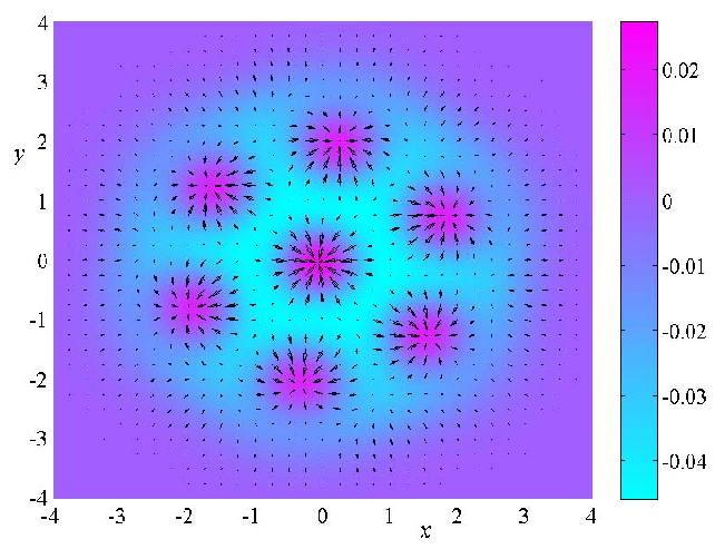
In the regime of intermediate SO coupling strength, the level spacing between single particle states within the same Landau level is suppressed as shown in Eq. (19). In the case that interactions are strong enough to mix energy levels with different angular momenta in the same lowest Landau level but not among different Landau levels, condensates do not keep rotation symmetry any more. The calculated phase boundary of interaction strength $\beta$ v.s. SO coupling strength $\alpha$ is plotted in Fig. 2. In this regime, the distributions are no long concentric but split into multi-centers and finally form a triangular skyrmion lattice structure as calculated in Refs. [54], [44]. This 2D skyrmion lattice structure is a characteristic feature brought by SO coupling.

If interactions are strong enough to mix states in different Landau levels, then the influence of the confining trap is negligible. The condensate configurations in the free space was calculated beyond the mean-field GP equation level in Ref. [27]. Bosons select the superposition of a pair of states with opposite momenta $\vec{k}$ and $-\vec{k}$ on the low energy Rashba ring to condense. These spin eigenstates of these two states are orthogonal, thus the condensate can avoid the positive exchange interactions. As is well known, avoiding exchange energy is the main driving force towards BEC. For spin-independent interactions, the condensate wavefunctions exhibit degeneracy at the Hartree-Fock level regardless of the relative weight between these two plane-wave components. This is a phenomenon of “frustration”. Quantum zero-point energy from the Bogoliubov quasi-particle spectra selects an equal weight supposition through the “order-from-disorder” mechanism. Such a condensate exhibits spin-spiral configuration.

Various literatures have also studied the case of spin-dependent interactions in which the Hartree-Fock theory is already enough to select either the spin-spiral state, or, a ferromagnetic condensate with a single plane-wave component [37, 38].

Next we review the condensates with the 3D Weyl SO coupling in the harmonic trap. The corresponding GP equation is very similar to Eq. (31) of the Rashba case. Only slight modifications are needed by replacing the spatial dimension 2 with 3, and by replacing the Rashba term with $-i\hbar\lambda_{W}\vec{\nabla}\cdot\vec{\sigma}$. Amazingly, in this case condensate wavefunctions exhibit topological structures in the quaternionic representation [68].

Ultracold atoms in a rotating trap share similar physics of electrons subject to magnetic fields due to the similarity between Lorentz and Coriolis forces. Depending on the experimental implementations of rotation, Hamiltonians can be of different types [79, 75, 76]. As pointed out in Ref. [75], because the current experiment setup breaks rotation symmetry, rotating SO coupled BECs is time-dependent in the rotating frame, which is a considerably more complicated problem than the usual rotating BECs. Nevertheless, below we only consider the situation of the isotropic Rashba SO coupling, such that it in principle can be implemented as a time-independent problem in the rotating frame.

The effect of rotation should be described by the standard minimal substitution method as presented in Ref. [79]. The non-interacting part of the Hamiltonian is

where $\vec{A}=m\Omega_{z}\vec{r}\times\hat{z}$, and the last term is the centrifugal potential due to rotation.

Note that due to the presence of SO coupling, we should carefully distinguish the difference between mechanical and canonical angular momenta. The mechanical one should be defined according to the minimal substitution as

where $L_{z}$ is the usual canonical angular momentum. Expanding Eq. (56), it is equivalent to Eq. (1) plus the term of angular velocity $\Omega_{z}$ coupling to $L^{mech}$ as

Thus in the rotating frame, the effect of $\Omega_{z}$ is not only just $\Omega_{z}L_{z}$ as usual, but also an extra effective radial Zeeman term as

Such a term is often missed in literatures. As will be shown below, it affects the ground state vortex configurations significantly and thus should not be overlooked.

To make the model more adjustable, an external spatially dependent Zeeman field $\vec{B}_{ex}=B\vec{r}$ is intentionally introduced as

which shares the same form as Eq. (59). Experimentally, such a Zeeman field can be generated through coupling two spin components using two standing waves in the $x$ and $y$-directions with a phase difference of $\frac{\pi}{2}$. The corresponding Rabi coupling is

In the region of $|x|,|y|\ll 2\pi/k_{L}$, it reduces to the desired form of Eq. (60) with $B=\Omega^{\prime}k_{L}$. Such a term compensates the non-canonical part of the mechanical momentum in $H_{rot}$, which renders the model adjustability in a wider range.