Effective Polyakov line action from the relative weights method
Abstract
We apply the relative weights method (arXiv:1209.5697) to determine the effective Polyakov line action for SU(2) lattice gauge theory in the confined phase, at lattice coupling and lattice spacings in the time direction. The effective action turns out to be bilinear in the fundamental representation Polyakov line variables, with a rather simple expression for the finite range kernel. The validity of this action is tested by computing Polyakov line correlators, via Monte Carlo simulation, in both the effective action and the underlying lattice theory. It is found that the correlators in each theory are in very close agreement.
Keywords:
Confinement,lattice gauge theoriespacs
11.15.Ha, 12.38.AwI Introduction
The Polyakov line action (PLA) is an action obtained from lattice gauge theory when all degrees of freedom are integrated out, under the constraint that the Polyakov line holonomies are held fixed. There are some indications [1, *Mercado:2012ue, 3, 4, 5] that the sign problem in this theory, at non-zero chemical potential, may be more tractable than the sign problem in the underlying lattice gauge theory (for a review, cf. [6]), and if so it could provide us with a new tool for investigating the QCD phase diagram. It is fairly straightforward, given the PLA at chemical potential , to introduce a non-zero chemical potential, as we discuss in section V. The problem we address here is how to extract the PLA from the underlying lattice gauge theory at .
This article is a follow-up to ref. [7], which presented a novel “relative weights” technique for deriving the PLA, based on a method used previously in studies of the Yang-Mills vacuum wavefunctional [8, *Greensite:1988rr]. The method was tested at strong couplings, where the answer is known, and a conjecture for the action at a weaker coupling, for SU(2) pure gauge theory at and inverse temperature lattice spacings, was presented. This conjecture was based, however, on a study limited to fairly atypical regions of field configuration space. Below we will apply the method in the region expected to dominate the path integral, and a rather different (and in fact simpler) action from the one conjectured in ref. [7] emerges. As a crucial test of the derived PLA, we compute the two-point Polyakov line correlator from Monte Carlo simulations of both the PLA and the underlying gauge theory. These correlators will be seen to agree quite accurately. Our effective PLA turns out to be only bilinear in the Polyakov line variables, with a simple expression for the finite range kernel.
There have been a number of previous attempts to derive the PLA from lattice gauge theory at finite temperature. These include strong-coupling expansions [3], the Inverse Monte Carlo method [10, *Heinzl:2005xv], and the demon approach [12, *Wozar:2008nv]. All of these methods generate effective Polyakov line actions of varying degrees of complexity. We believe, however, that an accurate agreement of Polyakov line correlators in the confined phase, computed in the effective and underlying lattice gauge theories, has not been demonstrated in any of the previous studies, at least not beyond two or three lattice spacings in Polyakov line separation.
It should also be mentioned that there are a number of studies which are concerned with deducing the Polyakov line potential, with particular application to the deconfinement transition, c.f. [14] and references therein. There have also been efforts, e.g. [15], to express the fermion determinant in terms of a potential involving Polyakov lines. These studies do not arrive at a full PLA as defined above, and hence their focus is somewhat different from ours.
Our article is organized as follows: An improved version of the relative weights method is presented in section II below. The technique is applied to pure SU(2) gauge theory in section III, again at and , and the Polyakov line correlators of the derived PLA are compared to those of lattice gauge theory. Application to a gauge-Higgs theory, with a scalar matter field explicitly breaking global center symmetry, is presented in section IV. Section V contains our conclusions. The extension of our method to gauge theories with dynamical fermions is discussed in an appendix.
II The relative weights method
The relative weights method, as applied to deriving the PLA , was introduced in ref. [7]. The technique is particularly well adapted to computing path (or “directional”) derivatives of the effective action in the space of all Polyakov line configurations. A single configuration is a point in this space, where we specify the group-valued Polyakov line holonomies at each spatial point in a three-dimensional volume. Let be a path through this space of configurations, where parametrizes the path. The relative weights method computes the path derivative at some given . In this section we present a variant of the relative weights approach which, while equivalent to the original method of [7], is numerically more efficient.
In order to minimize minus signs later on, we adopt the convention that the Boltzmann weight is proportional to . Let be the lattice gauge action on an volume with coupling for the Wilson action. may contain pseudofermion or bosonic matter degrees of freedom, collectively denoted by . It is convenient to go to temporal gauge, so that all timelike link variables are set to the unit matrix except on a timeslice at . Then the PLA is defined as
| (1) |
Because of the residual symmetry in temporal gauge, it follows that can only depend on the eigenvalues of the matrices.
While the functional integration in (1) can only be carried out in special cases, e.g. via strong coupling and hopping parameter expansions valid a certain range of parameters, the ratio (or “relative weights”) evaluated at nearby configurations is calculable numerically. This fact enables us to compute path derivatives of .
Let us consider a set of Polyakov line configurations
| (2) |
corresponding to values of the path parameter
| (3) |
and define
| (4) |
to be the lattice action in temporal gauge with the timelike links at fixed to the -th member of the set (2). We also define
| (5) |
From (1), we have
| (6) | |||||
where indicates that the expectation value is taken from ensembles with Boltzmann factor . For sufficiently small ,
| (7) | |||||
and these should closely agree, for all , with the derivative evaluated at the central value of . We can then improve our estimate by making use of all configurations, taking the average of derivatives
| (8) |
The question then becomes which point in configuration space should be chosen for the computation, and which directional derivatives at this point should computed, in order to deduce . It is possible that the choice is not very important, and that is well approximated by the same simple expression everywhere in configuration space. However, if this is not the case, then calculating path derivatives in some very atypical corner of configuration space may lead to an approximate answer for which may be correct in that particular corner, but misleading in the bulk of configuration space.
In ref. [7] the path derivatives were computed using three types of sets (2) for SU(2) lattice gauge theory. These were (i) Polyakov lines which were constant in space, and the parameter was the amplitude of ; (ii) Polyakov lines which consisted of small plane wave fluctuations around a constant background, with ; and (iii) Polyakov lines in which varied as . Compared to thermalized timeslice configurations generated in a normal lattice Monte Carlo simulation, such configurations are very atypical. In a thermalized configuration in the confined phase, the Fourier components of the configuration are all of , where is the lattice volume of the D=3 dimensional timeslice, whereas in the special configurations just mentioned, one Fourier component (which may be the zero mode) is of . For computing the PLA at a strong lattice coupling, where this action can be evaluated via a strong coupling expansion, the atypical nature of the constant + plane wave, or pure plane wave configurations did not seem important, and the PLA deduced from the relative weights data was a close match to the known result. There was no similar result to compare to at , and although an expression for matching the results for was deduced from fitting the data, there is a concern that this expression might only be valid in the special region of configuration space where it was derived.
We will investigate the action in more typical regions of configuration space in the next section.
III Derivatives of in a thermalized background
The goal is to use the expression for the path derivative (8) to determine . However, if does not have a simple form everywhere in configuration space (and it may not), then it is at least required that we have a fairly accurate approximation to in the region which is important for the computation of observables, i.e. the region occupied by typical thermalized configurations . A set of timelike link configurations on the timeslice, generated by a numerical simulation of the underlying lattice gauge theory, is a sample of such configurations. Let us define, for the SU(2) gauge group that we will consider here,
| (9) |
where the sum runs over all wavevectors on a cubic lattice of volume , and are real-valued. Then we may consider calculating numerically, by the relative weights method, derivatives with respect to the Fourier components
| (10) |
in a background in which all other Fourier components are drawn from a thermalized configuration. By calculating the derivative for some range of , it is possible to extrapolate to small of order , which is the typical magnitude of a Fourier component in thermalized configurations. It is sufficient in practice to concentrate on the coefficients of the cosine terms in the Fourier expansion, since the sine terms give similar results. We then try to reconstruct from this information.
There are potentially two obstacles to this approach. First, there are as many independent Fourier components as there are lattice sites in the volume, and this is too many to calculate in practice. Secondly, it might be that the results are strongly dependent on the particular thermalized background which is used. Concerning the first obstacle, this will not be a problem if the derivatives with respect to have a simple dependence on the lattice momentum
| (11) |
which can be deduced from a small sample of all possible components. As for the second obstacle, this is not a problem if it turns out that the dependence of the final results on the particular choice of thermalized configuration is very weak.
III.1 Deriving the effective PLA
The first step in the extrapolation to small is to run a standard lattice Monte Carlo, stop at some thermalized configuration, and calculate all the Polyakov line holonomies,
| (12) | |||||
where , in that configuration. Define . We pick a particular wavevector which is specified by three integers with corresponding wavenumber components
| (13) |
and set the coefficient of , in the sine-cosine expansion of , to zero. Denote the modified array, with the term removed, as .
Next, construct a set of configurations with:
| (14) |
where is a constant chosen to be as small as possible, but still large enough to get some spread in the data. Typically .
The factor in (14) is introduced in order to keep , with rare exceptions, inside the range . Ideally one would like to leave all in the thermalized configuration unaltered, apart from the mode with , i.e. . At finite , however, this has the disadvantage that at many sites . To see this, note that , from which is derived, may come close to the limits at some sites, and at these sites the additional contribution may put the sum outside the allowed range by as much as . Moreover, by removing the mode, may already lie outside the range at some sites; this is especially true for . We must also allow for the fact that half of the are slightly greater than . For this reason we reduce the amplitude of the added thermalized configuration by a factor of (in our simulations we found sufficient). In the exceptional cases where still lies outside the allowed range, it is truncated to the nearest limit, i.e. .
We then construct the SU(2) variables, at each site, which have as the trace
| (15) |
where, to insure unitarity,
| (16) |
The calculation of proceeds as described above. For the choice of given above, it is easy to see that for a lattice of extension in the spatial directions
| (17) |
The results for the derivatives are found to depend only weakly on the choice of thermalized time slice (12) generated in an ordinary Monte Carlo run. The dependence is most pronounced at small , with the variance on the order of 2%. In practice we have averaged our results for over eighty independent time slices.


In Fig. 1 we display our results for the vs. at , and lattice spatial extension . (Note that, apart from Figs. 5 and 7, all our figures show data derived at an extension.) The underlying SU(2) lattice gauge theory is defined as a Wilson action on a periodic volume, at the coupling . The calculations were made, in this case, at lattice momenta with components , with the following triplets:
| (18) |
On this plot the data point displayed at is a factor of two smaller than the actual data value; this was done for reasons to be explained shortly.
The striking thing about this data is that, for lattice momenta , the data points clearly fall on a straight line. The second fact is that the data is linearly proportional to at these small values, as we see in Fig. 2. In this figure we divide by , at , and find that the data points coincide. The linearity of the derivative w.r.t. implies that the action itself is quadratic in these variables, leading to a simple bilinear form
| (19) |
where
| (20) |
This leads to derivatives
The relative factor of two in the and cases is due to the fact that , while . The data should extrapolate, as , to a value which is half the result at , which is why we have divided the derivative at by a factor of 2, when displaying these values on Figs. 1 and 2. The constants and are obtained from a linear fit to the data at , as shown in Fig. 1.11 1 In practice we fit the data for each , at , to the form . We then fit to straight lines, and the constants are extracted from the slopes, i.e. , and . The choice of as the lower limit is a potential source of systematic error, since the value for can vary up to when the lower limit is increased (the variation of is smaller). We find, however, that the choice of as the lower limit minimizes the reduced value of the linear fit.

It is clear that for , the -space kernel is . If this were true at all , then we would have in position space, where is the lattice Laplacian. However, a kernel of this kind is infinite range, which would violate one of the assumptions of the Svetitisky-Yaffe analysis (cf. [16]). In any case, deviates from linearity at small momentum. We therefore make an ansatz for the kernel which imposes the finite range restriction on in a simple way:
Given , is obtained by a Fourier transform of . To determine , we do a linear fit of the data
| (28) |
as shown in Fig. 3. Let the slope of the line be . Then, from (III.1),
| (29) |
and we choose to satisfy this condition as closely as possible. We then have at all .
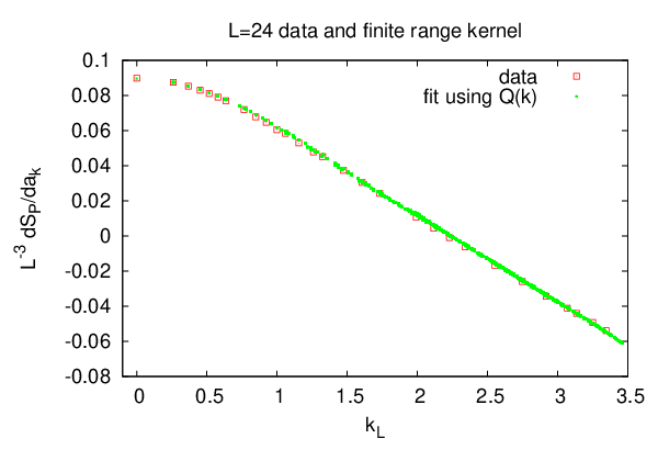
In Fig. 4 we plot the data shown in Fig. 1 together with the values computed for
| (30) |
(cf. eq. (III.1)) at . Agreement seems to be quite good in the entire range of .
We have repeated this analysis at smaller volumes of spatial extension . The results for are shown in Table 1. In Table 2 we record non-zero components of up to and lattice volume . For , the last entry in the table should be replaced by . The rest of the non-zero elements of are obtained from the table via permutation symmetry, , and reflection symmetry , among the coordinate components.
| 12 | 4.364(6) | 0.491(1) | 3.2 |
|---|---|---|---|
| 16 | 4.417(4) | 0.498(1) | 3.0 |
| 20 | 4.416(7) | 0.493(1) | 3.0 |
| 24 | 4.414(8) | 0.493(1) | 3.0 |
| 0 | 0 | 0 | 2.38760 |
| 1 | 0 | 0 | -0.22001 |
| 1 | 1 | 0 | -0.02357 |
| 1 | 1 | 1 | -0.00774 |
| 2 | 0 | 0 | -0.01279 |
| 2 | 1 | 0 | -0.00455 |
| 2 | 1 | 1 | -0.00246 |
| 2 | 2 | 0 | -0.00160 |
| 2 | 2 | 1 | -0.00111 |
| 3 | 0 | 0 | -0.00200 |
| 3 | 1 | 0 | -0.00121 |


III.2 Comparing the PLA to the underlying lattice gauge theory
We now have a concrete proposal for the effective Polyakov line actions at various spatial volumes ranging from to , and which correspond to an underlying lattice SU(2) gauge theory at on an lattice volume. The actions are specified by eqs. (19), (III.1), and the constants in Table I. Above the lattice volume , these actions are about the same.

The crucial question, of course, is whether these proposed Polyakov line actions are correct; they are certainly different from the action suggested in ref. [7], which was derived for gauge configurations in a rather unrepresentative region of configuration space. There is one obvious and essential test: Do the derived Polyakov line actions reproduce the Polyakov line correlator calculated in the corresponding lattice gauge theory? Thus we compute, via numerical simulation of the Polyakov line action at ,
| (31) |
and compare the result to the same observable obtained from standard lattice Monte Carlo at on an volume. The result for these four cases is shown in Fig. 5. Note that off-axis displacements are included, with -components of the displacement in the range .
The data in Fig. 5 is limited to displacements of magnitude lattice spacings, and it is interesting to consider larger displacements for larger lattices. This calls for higher statistics. In Fig. 6 we compare the results for obtained on a lattice for the effective theory, and on a lattice for the SU(2) gauge theory, again at . In this figure we show the results for displacements parallel to any one of the coordinate axes. The Lüscher-Weisz noise reduction method [17] was used in obtaining the Polyakov line correlator in the lattice gauge theory, while for the effective Polyakov line action the correlator was obtained from 38,400 configurations (about two orders of magnitude more than was used in Fig. 5).
The agreement of the correlators in the PLA and the underlying lattice gauge theory seen in Fig. 6 is extraordinary, and it persists down to magnitudes of order .22 2 The Polyakov line correlator derived from the Inverse Monte Carlo method in ref. [10, *Heinzl:2005xv] was displayed on a linear, rather than logarithmic, scale, and hence the precision of agreement with lattice gauge theory, in that approach, is difficult to judge. While this is not a proof that is the correct effective action, it is difficult to believe that agreement of Polyakov line correlators to this level of precision is coincidental.
IV Polyakov line action for an SU(2) gauge-Higgs system
We now add a scalar matter field in the fundamental representation of the gauge group, thereby breaking explicitly center symmetry. The simplest case is a fixed-modulus Higgs field, and for SU(2) gauge theory the action can be written in the following way:
| (32) |
where is SU(2) group-valued. The work of Fradkin and Shenker [18], itself based on a theorem by Osterwalder and Seiler [19], demonstrated that the Higgs region and the “confinement-like” regions of the phase diagram are continuously connected. Subsequent Monte Carlo studies found that there is only a single phase at zero temperature (there might have been a separate Coulomb phase), although there is a line of first-order transitions between the confinement-like and Higgs regions, which eventually turns into a line of sharp crossover around , cf. [20] and references therein. At the crossover occurs at , as seen in the plaquette energy data shown in Fig. 7. There is also a steep rise in the Polyakov line expectation value as increases past this point.

We will work at on a lattice volume, but this time at Higgs coupling , which places us in the “confinement-like” phase a little below the crossover point. For these parameters, the Polyakov line has a VEV of . Once again, we generate sets of thermalized Polyakov line holonomies, and compute as explained in the previous section.


The derivatives at are computed as before, and at each the results are simply proportional to . The constants are again extracted by a linear fit to the data. However, the data at is not strictly proportional to ; there is also an -independent constant contribution to the data. This fact can be seen in Fig. 8. The straight line is a best fit to evaluated at for in the range . The -intercept of this line does not pass through zero, but rather through . This implies that must contain a term which is linear in , i.e.
| (33) |
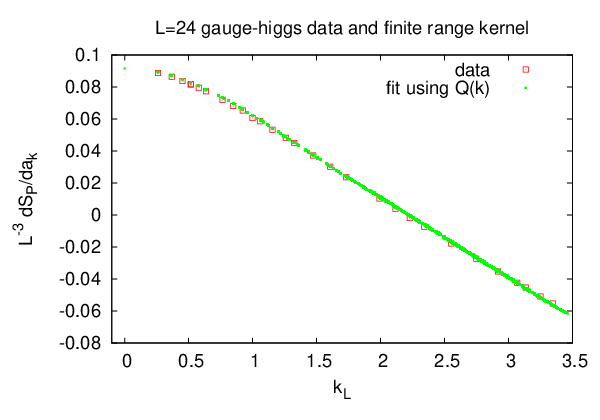
and it is clear from inspection that must equal to the -intercept in Fig. 8. It is also clear that only the mode contributes to the linear term, and is therefore invisible in the derivatives of at . We define again by (III.1), with determined as in the pure-gauge theory. The final set of parameters for the effective Polyakov line action is given in Table 3, and we plot the data, together with the quantity
| (34) |
in Fig. 9.
| 24 | .0236(14) | 4.447(9) | 0.501(1) | 3.2 |
|---|

As in the pure gauge theory, the crucial test is to see whether the Polyakov line correlator (31) found from numerical simulation of the gauge-Higgs theory (32) agrees with the same observable computed in the derived Polyakov line action (33). The results are shown in Fig. 10. In this case the agreement between the lattice gauge Higgs correlator (black diamonds) and the correlator of the effective action (blue triangles), while fairly close, is not perfect. However, the result for the effective action depends very sensitively on the value of , and of course there is an errorbar associated with this quantity. In our best fits, . With a little trial and error, one can find a value of for the effective effective action such that the corresponding correlator (red circles) agrees almost exactly with the gauge-Higgs value. This happens at a value which is not far outside our errorbars, about 1.4 away from .
V Conclusions
Motivated by the well-known sign problem, we have applied the relative weights method to determine the effective Polyakov line action for both pure and gauge-Higgs lattice SU(2) gauge theory. This effective action turns out to be a remarkably simple expression, which is bilinear in the Polyakov line variables :
with in the pure-gauge theory, and non-zero in the gauge-Higgs theory. Our results so far have been obtained at lattice coupling , and lattice spacings in the time direction. The effective action has been checked by computing Polyakov line correlators in both the effective theory and the underlying gauge theory, and we have found that these correlators agree quite well with each other. This is especially true in the pure gauge theory, where agreement persists down to correlator values of order . These results, together with previous checks in the case of strong coupling [7], inspire some confidence that the method works. The next immediate step will be to understand how the couplings of the effective theory evolve as a function of coupling and temperature .
In the longer term our interest is the sign problem, and to address that problem it will be necessary to derive the effective Polyakov line action corresponding to lattice SU(3) gauge fields coupled to matter at zero chemical potential. In lattice gauge theory fixed to temporal gauge, the chemical potential is introduced via the replacement
| (38) |
It is not hard to see that, to all orders in the strong coupling + hopping parameter expansion, the effective PLA obtained at is related to the action at by a simple substitution
| (39) |
We will assume that this identity holds in general. The strategy is then to apply one or more of the methods [1, *Mercado:2012ue, 3, 4, 5], which were developed for solving Polyakov line actions with a chemical potential, to our derived effective action. If the sign problem is tractable in the effective Polyakov line theory, as suggested by the earlier work cited above, then it may be possible to extract useful results regarding the QCD phase diagram.
Acknowledgements.
J.G. would like to thank Kim Splittorff for helpful discussions. J.G.’s research is supported in part by the U.S. Department of Energy under Grant No. DE-FG03-92ER40711. K.L.’s research is supported by STFC under the DiRAC framework. We are grateful for support from the HPCC Plymouth, where the numerical computations have been carried out. *Appendix A Dynamical Fermions
In this appendix we will just sketch how the relative weights algorithm can be applied in the case where there are two mass-degenerate dynamical fermions coupled to the gauge field.
Taking as the Dirac operator, and , the integration measure is
| (40) |
where is the Wilson (or other improved pure-gauge) action. Defining
| (41) |
we have
| (42) | |||||
where signifies, as before, the expectation value in a probability measure . The VEV can be evaluated via hybrid Monte Carlo, but in this case there is the question of how to evaluate the ratio of determinants in (42). In the most straightforward approach, defining and writing
| (43) |
it is not hard to see that
| (44) | |||||
Therefore
| (45) |
It is best not to evaluate the trace directly, because of the computational expense, but rather indirectly, by the method of “noisy pseudofermions” (c.f. section 8.4 in ref. [21]).
A way of completely avoiding in the observable is to introduce another set of pseudofermions , distinct from the pseudofermions used by hybrid Monte Carlo, so that we may write
| (46) |
Defining
| (47) |
we have
| (48) |
where refers to the expectation value in the measure proportional to
| (49) |
The final result for the relative weight is
| (50) |
Again, the expectation value would be computed via the usual hybrid Monte Carlo algorithm. Eq. (50) is to be used, as before, to compute path derivatives, hopefully leading to an expression for the effective PLA at . The PLA with a finite chemical potential would then be obtained from the substitution (39).
Apart from computation cost, we believe that the addition of dynamical fermions does not pose any problems of principle to the derivation of the effective Polyakov line action via the relative weights approach.
References
- [1] C. Gattringer, Nucl.Phys. B850, 242 (2011), arXiv:1104.2503.
- [2] Y. D. Mercado and C. Gattringer, Nucl.Phys. B862, 737 (2012), arXiv:1204.6074.
- [3] M. Fromm, J. Langelage, S. Lottini, and O. Philipsen, JHEP 1201, 042 (2012), arXiv:1111.4953.
- [4] G. Aarts and F. A. James, JHEP 1201, 118 (2012), arXiv:1112.4655.
- [5] J. Greensite and K. Splittorff, (2012), arXiv:1206.1159.
- [6] P. de Forcrand, PoS LAT2009, 010 (2009), arXiv:1005.0539.
- [7] J. Greensite, Phys.Rev. D86, 114507 (2012), arXiv:1209.5697.
- [8] J. Greensite, H. Matevosyan, Š. Olejník, M. Quandt, H. Reinhardt, and A.P. Szczepaniak, Phys.Rev. D83, 114509 (2011), arXiv:1102.3941.
- [9] J. Greensite and J. Iwasaki, Phys. Lett. B223, 207 (1989).
- [10] L. Dittmann, T. Heinzl, and A. Wipf, JHEP 0406, 005 (2004), arXiv:hep-lat/0306032.
- [11] T. Heinzl, T. Kaestner, and A. Wipf, Phys.Rev. D72, 065005 (2005), arXiv:hep-lat/0502013.
- [12] A. Velytsky, Phys.Rev. D78, 034505 (2008), arXiv:0805.4450.
- [13] C. Wozar, T. Kastner, B. H. Wellegehausen, A. Wipf, and T. Heinzl, PoS LATTICE2008, 257 (2008), arXiv:0808.4046.
- [14] A. Dumitru, Y. Guo, Y. Hidaka, C. P. K. Altes, and R. D. Pisarski, Phys.Rev. D86, 105017 (2012), arXiv:1205.0137.
- [15] K. Langfeld and G. Shin, Nucl.Phys. B572, 266 (2000), arXiv:hep-lat/9907006.
- [16] B. Svetitsky, Phys.Rept. 132, 1 (1986).
- [17] M. Luscher and P. Weisz, JHEP 09, 010 (2001), arXiv:hep-lat/0108014.
- [18] E. H. Fradkin and S. H. Shenker, Phys.Rev. D19, 3682 (1979).
- [19] K. Osterwalder and E. Seiler, Annals Phys. 110, 440 (1978).
- [20] C. Bonati, G. Cossu, M. D’Elia, and A. Di Giacomo, Nucl.Phys. B828, 390 (2010), arXiv:0911.1721.
- [21] C. Gattringer and C. B. Lang, Lect.Notes Phys. 788, 1 (2010).