A method for testing the cosmic homogeneity with Shannon entropy
Abstract
We propose a method for testing Cosmic homogeneity based on the Shannon entropy in Information theory and test the potentials and limitations of the method on Monte Carlo simulations of some homogeneous and inhomogeneous 3D point process in a finite region of space. We analyze a set of N-body simulations to investigate the prospect of determining the scale of homogeneity with the proposed method and show that the method could serve as an efficient tool for the study of homogeneity.
Keywords:
methods: numerical - galaxies: statistics - cosmology: theory - large scale structure of the Universe.August 24, 2026
1 Introduction
The cosmological principle which assumes that the Universe is statistically homogeneous and isotropic on very large scales is one of the fundamental pillars of modern cosmology. This can not be proved in a mathematical sense and can be only verified from observations and various predictions of the physical theories based on it. The cosmic microwave background is by far the best conclusive evidence in favour of isotropy (Penzias & Wilson, 1965; Smoot et al., 1992; Fixsen et al., 1996) which also strongly supports large scale homogeneity in the early Universe. Various other observations like the isotropy in angular distributions of radio sources (Blake & Wall, 2002) and the isotropy of the X-ray background (Peebles, 1993; Wu et al., 1999; Scharf et al., 2000) support the assumption of cosmic homogeneity on large scales. The isotropy does not by itself guarantee homogeneity and it implies homogeneity only when there is isotropy around every points. The present Universe is known to be highly inhomogeneous on small scales and there are important consequences if the inhomogeneities persist on large scales. The most important implication of inhomogeneities comes from the averaging problem in General Relativity through their effect on the large scale dynamics known as backreaction mechanism. The backreaction mechanism can cause a global cosmic acceleration without any additional dark energy component (Buchert & Ehlers, 1997; Schwarz, 2002; Kolb et al., 2006; Buchert, 2008) although it seems unlikely that this can explain all of it (Paranjape & Singh, 2008). The implications of inhomogeneities and backreaction for Cosmology are still considered to be important even if it does not provide an alternate explanation of dark energy (Paranjape, 2009; Kolb et al., 2010; Ellis, 2011).
The principle of cosmic homogeneity demands that the statistical properties of the observed galaxy distribution in a given finite volume does not depend on the location of that volume in the Universe. The statistical properties of galaxy distributions are characterized by the correlation functions (Peebles, 1980). The two point correlation function on small scales , is well described by a power law of the form , with correlation length and slope . vanishes at scales which is consistent with large scale homogeneity. However the problem with correlation function analysis is that it assumes a mean density on the scale of survey which is not a defined quantity below the scale of homogeneity. Most of the statistical tools for homogeneity analysis are based on the simple number counts in spheres of radius which is expected to scale as for a homogeneous distribution. The conditional density (Hogg et al., 2005; Sylos Labini, 2011a) measures the average density in these spheres which is expected to flatten out beyond the scale of homogeneity. The fractal analysis (Martinez & Jones, 1990; Coleman & Pietronero, 1992; Borgani, 1995) uses the scaling of different moments of to characterize the scale of homogeneity. Some of the studies carried out with these methods on different galaxy surveys claim to have found a transition to homogeneity on sufficiently large scales (Martinez & Coles, 1994; Guzzo, 1997; Martinez et al., 1998; Bharadwaj et al., 1999; Pan & Coles, 2000; Kurokawa et al., 2001; Hogg et al., 2005; Yadav et al., 2005; Sarkar et al., 2009; Scrimgeour et al., 2012) whereas some studies claim the absence of any such transition out to scale of the survey (Coleman & Pietronero, 1992; Amendola & Palladino, 1999; Sylos Labini et al., 2007; Sylos Labini et al., 2009a; Sylos Labini et al., 2009b; Sylos Labini, 2011b). The disagreements between various studies indicate the need for some alternative measures of homogeneity which could capture interesting information on different aspects of a homogeneous distribution and serve as complimentary and alternative tool to the existing methods in the literature. In the present work we introduce a method to asses homogeneity which is based on the evenness, a more general and robust aspect of any homogeneous distribution. We employ the Shannon entropy (Shannon, 1948) to measure the unevenness characterizing inhomogeneities in a distribution and explore the possibility of employing the proposed method for exploring the scale of homogeneity.
A brief outline of the paper follows. We describe our method and various effects in Section 2, describe the tests and the data in Section 3 and presents the results and conclusions in Section 4.
2 Method of analysis
Our method is based on the Shannon entropy in Information theory originally proposed by Claude Shannon to quantify the information content in strings of text.
In Information theory entropy is a measure of the amount of information required to describe the random variable. The Shannon entropy for a discrete random variable with outcomes is a measure of uncertainty denoted by defined as,
| (1) |
where is the probability distribution of the random variable . Increase in Shannon entropy increases the uncertainty and decreases the information about the knowledge of the random variable. Another interesting aspect of Shannon entropy is its entropy-maximizing property for an uniform distribution.
We propose a method to study inhomogeneities in a 3D distribution of
points. Given a set of points distributed in 3D we consider each
of the points as center and determine the number of
other points within a sphere of radius as,
| (2) |
where is the Heaviside step function and and are the radius vector of and points respectively. To avoid any edge effects we discard all the points as centers which lie within a distance from the survey boundary. Clearly the number of valid centers will decrease with increasing for any finite volume sample. We define a separate random variable for each radius which has possible outcomes each given by, with the constraint . Here is the density at the center. Note that for a given sample with a finite volume, is the maximum numbers of valid centers available at a radius i.e. there are no provision for projecting further another sphere of radius within the given volume.
The Shannon entropy associated with the random variable can be written as,
| (3) | |||||
where the base of the logarithm is arbitrary and we choose it to be . Note that in , and , is a just a label for a number and not an argument.
In an ideal situation when all the spheres around the valid centers are equally populated then one gets an uniform value of for all the centers maximizing the uncertainty. Then the Shannon entropy (equation 3 ) has its maximum value for radius . The relative Shannon entropy at any quantifies the degree of uncertainty in the knowledge of the random variable . When the knowledge about the random variable becomes most uncertain. The distribution of also become completely uniform when is reached. Equivalently one can use to quantify the information available in at any .
The joint Shannon entropy of a set of independent random variables is simply the sum of the individual entropies associated with each of the random variables. But if they are dependent then the total entropy is a sum of the conditional entropies. Entropy measures uncertainty in the random variable whereas the information is a difference in uncertainty that is a difference in entropies. The mutual information characterizes the reduction in the uncertainty in the one random variable due to the knowledge of the other.
In our case the mutual information between the random variables are always positive as the random variables are not independent due to the fact that the density measurements around centers at each radius are taken from the same finite volume sample. Given that the mutual information are always positive for correlated random variables, an increase in information in at one would lead to decrease in information in s at other values. Apart from the correlations from finite sample, the random variables could have extra correlations if the points are clustered or if the points are distributed in a preferred way. These extra correlations increase the mutual information in the random variables . The decrease of information in with increasing is evident irrespective of a homogeneous/inhomogeneous distribution but it would diminish differently depending on the nature and the degree of inhomogeneity present in the distribution. Maximum uncertainty or the complete loss of information in the knowledge of the random variable at a radius suggests that beyond the random variables would be independent and completely uninformative about each other. In an infinite perfectly homogeneous system if the set of spheres used for density measurements are completely independent then the random variables at each has no knowledge about each other making them maximally uncertain and devoid of any information. When no inhomogeneities are present due to other sources, the departure of from would be solely due to the correlations among caused by the finite volume of the sample. Given the other sources are present one would expect a larger departure of this ratio from and a more uneven distribution of . The scale where this departure levels up with indicates absence of any correlations among beyond that scale. But this ideal situation may never occur in an exact sense in a finite sample as the correlations between s introduced by the finite volume and confinement bias persists over the whole range of length scales. This would always give some residual information in even at the largest value of . But the mutual information content due to clustering or any other source of inhomogeneity are expected to diminish with increasing length scale provided a scale of homogeneity exist for the distribution. As the exact transition marked by may never happen in a finite volume sample so one could set a very small limiting value for to identify the scale of homogeneity. In our analysis we set this limit to .
2.1 Effects of clustering, intrinsic inhomogeneity and finite volume
Clustering of the points is the most important source of correlations
between the random variables . Clustering produces fluctuations
in which is directly related to the fluctuations in
. When the points are clustered we expect on average
number of points in a volume where is
given by,
| (4) |
Here is the mean density of the distribution and is the volume of the sphere used. The first
term has fluctuations from the Poisson noise of the same order. The
Poisson noise rapidly decreases with increasing and is only
important on small scales. If the distribution itself is
intrinsically inhomogeneous then Poisson noise will be modulated
according to the spatially dependent intensity parameter .
The second term takes into account of clustering of the points. The
variance of is,
| (5) |
Going back to our definition of , the fluctuations in this quantity is closely related to the fluctuations in . The variance in is,
| (6) |
which is times the normalized variance of .
One can quantify the correlations of any two random variables at two different by estimating their covariance. The correlation coefficient is,
| (7) |
where the indices and takes value between to . Here is the total number of values used in the analysis. In this case we have a positive correlation between and and the correlations would be higher when the differences between and are smaller. The random vector has equally likely outcomes and in principle one can estimate the full covariance matrix of all the random variables at different s to compute their correlations.
Even in the absence of any clustering and inhomogeneity one would expect a positive correlations between the random variables as their probability distribution is derived from the same finite volume sample. The set of centers at each is a subset of the centers at the preceding . More specifically all the set of centers at each is a subset of the set of the centers at the smallest implying the spheres at different share some common regions. The fractional amount of share is larger when the difference between is smaller thereby introducing larger correlations between the s from neighboring values. So the finite volume introduces correlations between the random variables at different which increases the mutual information in the random variables.
2.2 Effects of overlapping
One should also keep in mind that the spheres used for density measurements are not independent and could share large overlapping regions. At each we use a finite set of spheres for density measurements. In general these spheres overlap with each other. The probability that a random point drawn out of the distribution would lie in a particular sphere is where is the total number of points in the distribution. The probability that the randomly drawn point would appear somewhere in the sample is . If the spheres are disjoint then at any there are outcome of this experiment i.e the point would lie either in any one of the spheres or somewhere in the sample outside the spheres. But given the fact that the spheres overlap the point could also appear at the intersections of multiple spheres. Given a finite sample the total probability can be written as,
| (8) | |||||
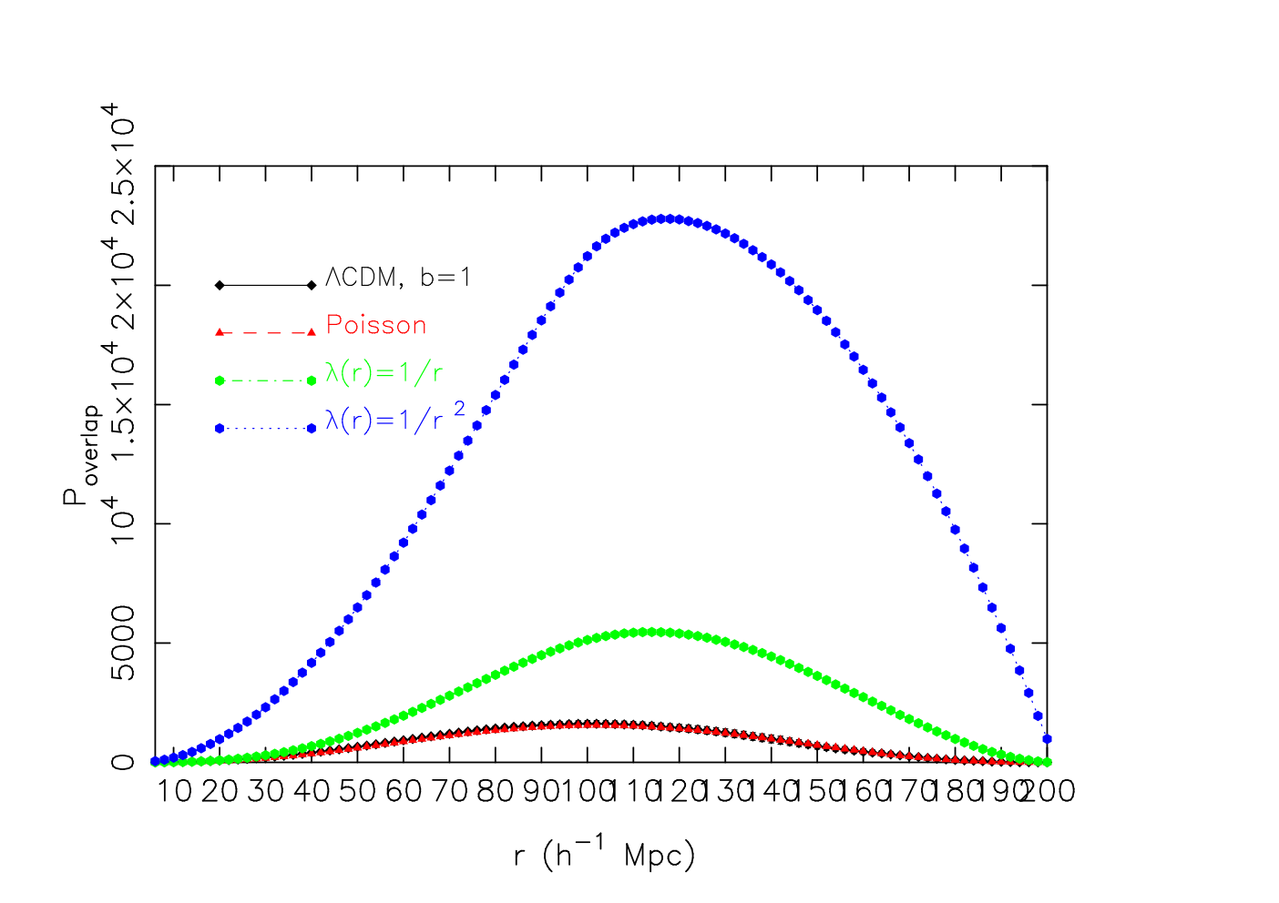
The first sum in above equation gives the sum of probabilities for individual spheres provided they are disjoint. As the spheres overlap one needs to take into account the probabilities for all the possibilities. The second sum is over all distinct pairs of spheres, third sum is over all distinct triples of spheres and so forth. The last term which gives the probability that the point would come up in a region outside the union of spheres is important only at small and becomes insignificant afterwards. It may be noted that in an overlapping scenario the different terms in equation 8 can be much larger than but when summed together they will always give . In equation 8, contains all the terms from overlapping spheres and successive terms in has alternate sign . At smaller the most dominant contribution to comes from all pairs of overlapping spheres. The contribution from all triples of overlapping spheres would be the next dominant term and so on. Thus at smaller all the individual sums in are different and the magnitude of each sum is lesser than its preceding sum resulting into a positive value of . New sums appear in with increasing thereby increasing its value. But at the same time the differences between the successive sums starts decreasing due to larger overlap thereby decreasing the value of . There is a competition between this two effect and initially the first effect is more dominant than the second leading to an overall increase in with increasing . As we increase the radius the numbers of valid centers decreases and they preferentially get more confined near the center of the sample. Due to the finite volume of the sample ultimately the second effect will dominate on some scale depending on the size of the finite sample and also depending on the nature of inhomogeneity to some extent. For example the confinement bias is expected to be even higher for an inhomogeneous distribution which preferentially has more particles residing near the center of the sample. When the differences between the successive sums become smaller then there would be a larger net cancellation leading to smaller values of . As the second effect starts dominating the first one, the value of would start decreasing and finally on the scale of the largest sphere that would fit inside the finite sample, all the individual terms in all the individual sums in would be of the same order i.e. . This would lead to a very large mutual cancellation of all the sums in decreasing its value to or . This finite volume effect eventually introduces an artificial evenness in the distribution of at some depending on the sample size. We see that the effect of overlapping starts dominating much before the scale of the largest possible sphere (Figure 1) making an interpretation difficult on large scales. We note that all the other methods of testing homogeneity based on count in spheres are also affected by the same problem making the interpretations on large scales equally difficult.
In order to avoid these complicacy of correlations introduced by the overlapping of the spheres we also consider non-overlapping spheres of different radii. But the statistics becomes too noisy due to very small number of independent spheres at progressively larger radii which consequently prohibits us to address the issue of homogeneity on large scales.
A point of caution in this context is that in our method at very large length scales does not necessarily indicate a real transition to homogeneity which is an obvious outcome forced by the confinement bias resulting from the finite volume of the sample. But with a large enough sample which ensures spheres upto a sufficiently large without significant confinement of the centers could detect the scale of homogeneity if the transition happens before the scale where the confinement bias completely dominates the statistics.
3 Tests on homogeneous, inhomogeneous and clustered distributions
In order to study the prospects and limitations of the proposed method we carry out some preliminary tests by applying it to some simple distributions. We consider (i) homogeneous distribution without any clustering, (ii) inhomogeneous distribution without any clustering and (iii) strongly clustered distribution.
In above three cases the unevenness in type (i) is only due to Poisson noise. The unevenness in type (ii) distribution is controlled by Poisson noise too but it has the additional complexity that the contribution to the unevenness is governed by the distribution of the spatially dependent intensity parameter . In type (iii) distribution both Poisson noise and the clustering together contributes to the unevenness.
For the first two types we generate a set of Monte Carlo realizations of some simple homogeneous and inhomogeneous point process. For the third type we use a set of N-body simulations where the points are strongly clustered.
3.1 Monte Carlo simulations of homogeneous and inhomogeneous point processes
We generate a set of Monte Carlo realizations of different types of homogeneous and inhomogeneous distributions.
For the sake of simplicity we consider some simple radial density distributions where (i) , (ii) and (iii) . is a normalization constant. The distributions in (i) and (ii) are inhomogeneous Poisson distributions which are isotropic about only one point and the inhomogeneities in these distributions persist on all scales. The distribution in (iii) is a homogeneous Poisson point process which has a constant density everywhere.
Enforcing the desired number of particles within radius one can turn the radial density function into a probability function within to which is normalized to one when integrated over that interval. So the probability of finding a particle at a given radius is which is proportional to the density at that radius implying more particles in high density regions.
We generate the Monte Carlo realizations of these distributions using a Monte Carlo dartboard technique. The maxima of the function in is at in (i) and (ii) whereas in (iii) it is same and constant everywhere. We label the maximum value of as . We randomly choose a radius in the range and a probability value is randomly chosen in the range . The actual probability of finding a particle at the selected radius is then calculated using expression for and compared to the randomly selected probability value. If the random probability is less than the calculated value, the radius is accepted and assigned isotropically selected angular co-ordinates and , otherwise the radius is discarded. In this way, radii at which particle is more likely to be found will be selected more often because the random probability will be more frequently less than the calculated actual probability. We choose in unit and . We generate realizations of each of the above density distributions and analyze them separately with the method described in section 2.
3.2 N-body simulations
We simulate the dark matter distribution using a Particle-Mesh (PM) N-body code. The simulations use particles on a mesh and cover a comoving volume of . We use for the cosmological parameters along with a CDM power spectrum with spectral index and normalization (Komatsu et al. 2009). A simple “sharp cutoff” biasing, scheme (Cole, Hatton & Weinberg, 1998) was used to extract particles from the simulations that are biased relative to the dark matter and are labelled as galaxies. The bias parameter of each simulated biased sample was estimated using the ratio
| (9) |
where and are the galaxy and dark matter two-point correlation functions respectively. This ratio is found to be constant at length-scales and we use the average value over . We use this method to generate galaxy samples with bias values and . We run the simulation for three different realizations of the initial density fluctuations and extract biased samples from each of them. We extract randomly particles from three non overlapping spherical regions of radius from each of the simulation boxes giving us total nine samples for each of the bias values. The numbers and and the specific spherical geometry are chosen just to maintain the uniformity in all the analysis presented here. Generally one can choose any number of particles and any geometry for the samples.
4 Results and Conclusions
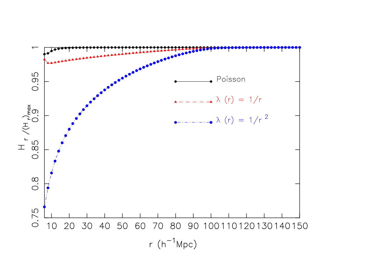
In the Figure 2 we show the variations of with distance for some homogeneous and inhomogeneous distributions described in subsection 3.1. For the Poisson distribution the value of shows a small departure from at smaller values of which decreases with increasing . The ratio reaches a value at . As the points are uncorrelated, the Void Probability function (White, 1979) for a homogeneous Poisson distribution is . It is expected that such a distribution would become homogeneous on a scale , which is a measure of the average size of voids in the distribution. Since the correlations between the random variables in the homogeneous Poisson distribution mainly comes from the finite volume effect one would expect a lesser amount of mutual information in the set of random variables and consequently a faster information leakage but the information in i.e. would never be exactly zero due to persistence of the finite volume correlations at all .
The values at smaller values shows relatively larger departure from for both the inhomogeneous distributions considered here. The ratio has a larger departure for the distribution with than the distribution with on all scales. This shows that the ratio describes the degree of inhomogeneity present in two different anisotropic distributions in correct order. Both these distributions are only isotropic about one point and have a radial density distribution which does not allow them to be homogeneous on any scales. The ratio at for both of them simply shows the importance of confinement bias which ultimately is expected to take over the situation at some depending on the sample size and type of inhomogeneity present. The confinement bias gets a larger boost in both of these distributions (Figure 1) as there are already more particles preferentially located near the center of the samples. This effect produces larger overlap and hence larger mutual information are stored in the random variables from neighbouring s. Consequently this accelerates the leakage of information in with increasing finally forcing the ratio . It may be noted that for the homogeneous Poisson distribution there are no such additional boost coming from preferential deposition and further there are no extra correlations due to clustering. The transition is reached there at a much before the scale where the confinement bias play a dominant role indicating a real transition to homogeneity.
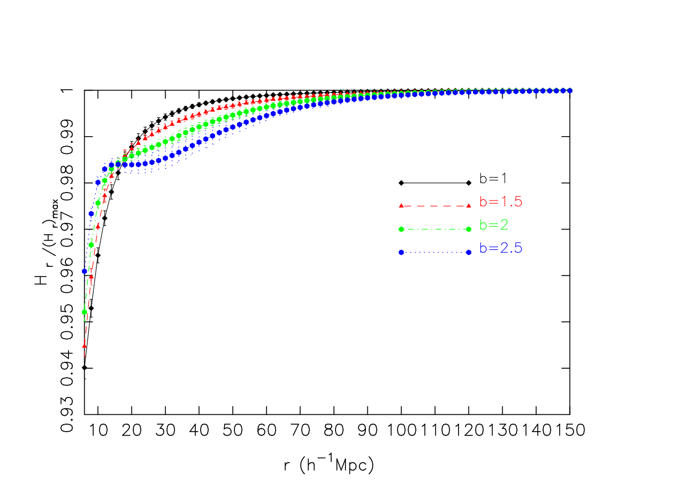
In the Figure 3 the variations of with distance are shown for CDM N-body simulations with different linear bias values. The assumption of linear bias holds reasonably well on large scales. Different types of galaxies are biased differently with respect to the dark matter and the inhomogeneities in the distributions of different types of galaxies could be modulated by their bias values. We would also like to investigate here how well the ratio can track the variation in inhomogeneities in a distribution on different scales and give some useful information about the characteristics of the inhomogeneities present in them. We see that the ratio initially depart from at small for all the distributions with higher bias values showing systematically lesser inhomogeneity (lesser information in ) than lower bias values. In the unbiased CDM model the centers used for calculating are residing in all types of environments (clusters, sheets, filaments and voids). The fact that the centers are distributed across different types of nonlinear structures increases the unevenness in the distribution of and the mutual information in . Whereas with increasing bias values the particles in a biased distribution preferentially represent progressively higher density peaks in the density field homogenizing the distribution on the corresponding length scales. This is primarily due to the fact that in a biased distribution the centers are located in less diverse environments. A complete reversal of this behaviour is seen at after which with increasing bias values the distributions systematically show larger inhomogeneity and more information in at all scales until they eventually merge to . This behaviour is related to the fact that increasing the radius beyond the typical scale of the nonlinear structures in the biased distributions would lead to larger disparity in and values and hence the larger inhomogeneities. The scales corresponding to the reversal in the behaviour of ratio corresponds to the typical scale of the nonlinear structures present in the biased distributions. Further on large scales the correlation functions in biased distributions are times larger than the in unbiased distributions introducing larger correlations among all the random variables at larger . Eventually all the curves merge to in the range with the difference that the transition appears to happen at a relatively larger values for larger bias. Although this can not be emphasized due to the size of the overlapping error bars at those length scales. It may be noted that the inhomogeneities in the CDM model with different biases are much smaller as compared to the inhomogeneous radial density distributions given by . The information in for a Poisson distribution mostly comes from the finite volume effect whereas the very large mutual information in the random variables in two inhomogeneous distributions is the combined outcome of finite volume correlations and large degree of confinement bias. In the unbiased and biased CDM models the mutual information are generated by correlations from confinement bias and clustering together. It may be noted that the confinement biases are much smaller and very similar in the CDM models and the homogeneous Poisson distributions (Figure 1). The confinement biases become very large in the two anisotropic distributions considered here which eventually force the ratio to at some scales.
If a scale of homogeneity exists then ideally one would expect a naturally emerging evenness in when the spheres of that radius around each centers statistically include similar numbers of different types of nonlinear structures. So provided that the correlations introduced by the finite volume of the sample and the confinement bias are much smaller compared to the correlations induced by clustering then the leakage of information in would ideally track the variation of inhomogeneity in the distribution with scale . But unfortunately in a real situation one has to also deal with the correlations due to finite volume and confinement bias modulating the information in or the evenness of . We find that the confinement bias could start to dominate even much before the scale defined by the largest sphere included in any finite sample (Figure 1). The degree of correlations introduced among s would also depend on the type of inhomogeneity present in the distribution specially if it is overpopulated near the center of the sample with respect to the rest of the volume resulting into larger overlap between the spheres. When dealing with galaxy redshift surveys one has to also properly take into account the different selection effects involved, redshift space distortions and the specific geometry of the samples. We plan to carry out analysis in the publicly available catalogues from large galaxy redshift surveys (e.g. 2dFGRS, Colles et al. 2001; SDSS, Stoughton et al. 2002; 2MASS, Huchra et al. 2012) in future works and investigate these issues further. It may be noted here that a caveat of our method is we assume that we always have access to the data samples on a spatial hypersurface of constant time. Though this assumption is approximately valid in case of low redshift galaxy samples in the nearby Universe or data samples from a snapshot of N-body simulations, it is not strictly true as the entire observational samples do not consist of objects on a constant time hypersurface but rather on a light cone. Taking this into account it is hard to distinguish radial inhomogeneity from time evolution without assuming a cosmological model. Consequently this could make an inhomogeneous but isotropic model (e.g. anti-Copernican void models) to look like a homogeneous one on large scales. Fortunately these models can be constrained with other observations such as SNe, CMB, BAO and measurements of Hubble parameter (Zibin et al., 2008; Clifton et al., 2008; Biswas et al., 2010; Clarkson, 2012).
Finally we note that the method presented here has the desired ability to characterize inhomogeneities and their variations on different length scales in any 3D distribution of points. The method has the potential to successfully identify any existing scale of homogeneity given a sufficiently large volume which can ensure negligible confinement bias and less effective overlap between the spheres upto large length scales. Given the large survey volumes that are currently available from the modern redshift surveys the method could provide an efficient tool for exploring the issue of Cosmic homogeneity.
Acknowledgment
The author thanks Somnath Bharadwaj for useful comments and discussions. The author would also like to thank an anonymous refree for insightful comments about the paper. The author acknowledges the Alexander von Humboldt Foundation for financial support and the Computing Center of the Max Planck Society in Garching (RZG) for the computing facilities provided for the work.
References
- Amendola & Palladino (1999) Amendola, L., & Palladino, E. 1999, ApJ Letters, 514, L1
- Biswas et al. (2010) Biswas, T., Notari, A., & Valkenburg, W. 2010, JCAP, 11, 30
- Bharadwaj et al. (1999) Bharadwaj, S., Gupta, A. K., & Seshadri, T. R. 1999, A&A, 351, 405
- Borgani (1995) Borgani, S. 1995, Physics Reports, 251, 1
- Blake & Wall (2002) Blake, C., & Wall, J. 2002, Nature, 416, 150
- Buchert (2008) Buchert, T. 2008, General Relativity and Gravitation, 40, 467
- Buchert & Ehlers (1997) Buchert, T., & Ehlers, J. 1997, A&A, 320, 1
- Clarkson (2012) Clarkson, C. 2012, Comptes Rendus Physique, 13, 682
- Clifton et al. (2008) Clifton, T., Ferreira, P. G., & Land, K. 2008, Physical Review Letters, 101, 131302
- Cole, Hatton & Weinberg (1998) Cole, S., Hatton, S., Weinberg, D. H., & Frenk, C. S. 1998, MNRAS, 300, 945
- Coleman & Pietronero (1992) Coleman, P. H., Pietronero, L. 1992, Physics Reports, 213, 311
- Colles et al. (2001) Colles, M. et al.(for 2dFGRS team) 2001,MNRAS,328,1039
- Ellis (2011) Ellis, G. F. R. 2011, Classical and Quantum Gravity, 28, 164001
- Fixsen et al. (1996) Fixsen, D. J., Cheng, E. S., Gales, J. M., et al. 1996, ApJ, 473, 576
- Guzzo (1997) Guzzo, L. 1997, New Astronomy, 2, 517
- Hogg et al. (2005) Hogg, D. W., Eisenstein, D. J., Blanton, M. R., Bahcall, N. A., Brinkmann, J., Gunn, J. E., & Schneider, D. P. 2005, ApJ, 624, 54
- Huchra et al. (2012) Huchra, J. P., Macri, L. M., Masters, K. L., et al. 2012, ApJS, 199, 26
- Kolb et al. (2006) Kolb, E. W., Matarrese, S., & Riotto, A. 2006, New Journal of Physics, 8, 322
- Kolb et al. (2010) Kolb, E. W., Marra, V., & Matarrese, S. 2010, General Relativity and Gravitation, 42, 1399
- Komatsu et al. (2009) Komatsu, E., et al. 2009, ApJS, 180, 330
- Kurokawa et al. (2001) Kurokawa, T., Morikawa, M., & Mouri, H. 2001, A&A, 370, 358
- Martinez & Jones (1990) Martinez, V. J., & Jones, B. J. T. 1990, MNRAS, 242, 517
- Martinez & Coles (1994) Martinez, V. J., & Coles, P. 1994, ApJ, 437, 550
- Martinez et al. (1998) Martinez, V. J., Pons-Borderia, M.-J., Moyeed, R. A., & Graham, M. J. 1998, MNRAS, 298, 1212
- Pan & Coles (2000) Pan, J., & Coles, P. 2000, MNRAS, 318, L51
- Paranjape & Singh (2008) Paranjape, A., & Singh, T. P. 2008, Physical Review Letters, 101, 181101
- Paranjape (2009) Paranjape, A. 2009, arXiv:0906.3165
- Penzias & Wilson (1965) Penzias, A. A., & Wilson, R. W. 1965, ApJ, 142, 419
- Peebles (1993) Peebles, P. J. E. 1993, Principles of Physical Cosmology. Princeton, N.J., Princeton University Press, 1993
- Peebles (1980) Peebles, P. J. E. 1980, The large scale structure of the Universe. Princeton, N.J., Princeton University Press, 1980, 435 p.,
- Sarkar et al. (2009) Sarkar, P., Yadav, J., Pandey, B., & Bharadwaj, S. 2009, MNRAS, 399, L128
- Scharf et al. (2000) Scharf, C. A., Jahoda, K., Treyer, M., et al. 2000, ApJ, 544, 49
- Schwarz (2002) Schwarz, D. J. 2002, arXiv:astro-ph/0209584
- Scrimgeour et al. (2012) Scrimgeour, M. I., Davis, T., Blake, C., et al. 2012, MNRAS, 3412
- Shannon (1948) Shannon, C. E. 1948, Bell System Technical Journal, 27, 379-423, 623-656
- Smoot et al. (1992) Smoot, G. F., Bennett, C. L., Kogut, A., et al. 1992, ApJ Letters, 396, L1
- Stoughton et al. (2002) Stoughton, C., et al. 2002, AJ, 123, 485
- Sylos Labini et al. (2007) Sylos Labini, F., Vasilyev, N. L., & Baryshev, Y. V. 2007, A&A, 465, 23
- Sylos Labini et al. (2009a) Sylos Labini, F., Vasilyev, N. L., & Baryshev, Y. V. 2009a, Europhysics Letters, 85, 29002
- Sylos Labini et al. (2009b) Sylos Labini, F., Vasilyev, N. L., Pietronero, L., & Baryshev, Y. V. 2009b, Europhysics Letters, 86, 49001
- Sylos Labini (2011a) Sylos Labini, F. 2011a, Classical and Quantum Gravity, 28, 164003
- Sylos Labini (2011b) Sylos Labini, F. 2011b, Europhysics Letters, 96, 59001
- White (1979) White, S. D. M. 1979, MNRAS, 186, 145
- Wu et al. (1999) Wu, K. K. S., Lahav, O., & Rees, M. J. 1999, Nature, 397, 225
- Yadav et al. (2005) Yadav, J., Bharadwaj, S., Pandey, B., & Seshadri, T. R. 2005, MNRAS, 364, 601
- Zibin et al. (2008) Zibin, J. P., Moss, A., & Scott, D. 2008, Physical Review Letters, 101, 251303