Advanced Interacting Sequential Monte Carlo Sampling for Inverse Scattering

EM scattering measurements have been achieved ever since radar invention [3]. Briefly speaking, EM scattering is the standard phenomenon that occurs when an object is exposed to an EM wave and disperses incident energy in all directions (scattering is this spatial distribution of energy). Some energy is scattered back to the source of the wave. It constitutes the radar echo of the object, the intensity of which results from the radar cross section (RCS) of the object. More precisely, RCS is defined by:

It quantifies the scattering power of an object, i.e. the ratio between the scattered power density $\mathbf{E}_{\mathrm{scat}}$ at the receiver and the power density of the incident wave at the target (with $R$ the radar-object range). It depends on the wave polarization and frequency. The $4\pi R^{2}$ term takes into account the radiated spherical wave. Implicitly, (1) requires that the incident wave is planar ($R\to+\infty$). Practically, it is possible to measure the RCS at limited ranges with a sufficient accuracy. It is usually achieved in indoor RCS test chambers, also called anechoic chambers. There, interferences can be limited by microwave absorbing materials (see figure 1).

In the article, we consider that an object or mock-up is illuminated by a radar, i.e. a single antenna or a more complex device (such as the antenna array of figure 1) that fulfills to a certain extent directivity and far-field conditions [19]. Herein the radar system is monostatic, which means that the transmitter and receiver are collocated. Its common principle is described in figure 2. Considering that the radar illuminates the object at a given incidence with a quasi-planar monochromatic continuous wave (CW) of frequency $f$ (incident electric field $\mathbf{E}_{\mathrm{inc}}$), the object backscatters a CW to the radar (scattered electric field $\mathbf{E}_{\mathrm{scat}}$) at the same frequency. With an appropriate instrumentation system (radar, network analyzers, etc.) and a calibration process, it is possible to measure the complex scattering coefficient, which can be roughly defined by: $\mathcal{S}=\frac{\mathbf{E}_{\mathrm{scat}}}{\mathbf{E}_{\mathrm{inc}}}$. It sums up the EM scattering, indicating the wave change in amplitude and phase. $\mathcal{S}$ is closely linked to the RCS, with: $\sigma_{s}=|\mathcal{S}|^{2}$. It is important to notice that the scattering coefficient quantifies a global characteristic of the whole object-EM wave interaction in specific conditions (incidence, frequency, etc.). It is possible to measure the scattering coefficient for different transmitted and received polarizations.

Let assume the following conventional RCS acquisition mode, widely used in Inverse Synthetic Aperture Radar (ISAR) imaging. It consists in measuring various complex scattering coefficients $\mathcal{S}$:

• -

  at different wave frequencies: $f\in\{f_{1},f_{2},\cdots,f_{K_{f}}\}$, for $K_{f}$ successive discrete frequencies. Basically, it consists in a series of transmitted narrow-band pulses, commonly known as SFCW (Stepped Frequency Continuous Wave) burst [20].

• -

  at different incidence angles: $\theta\in\{\theta_{1},\theta_{2},\cdots,\theta_{K_{\theta}}\}$, for $K_{\theta}$ different incidence angles (object rotation with a motorized rotating support).

• -

  at different (transmitted and received) linear polarizations: $\mathrm{pol}\in\{HH,VV\}$, meaning respectively, horizontally and vertically polarized both at microwave emission and reception.

Let call $\mathcal{M}$ the complete measurement, set of $2\cdot K_{f}\cdot K_{\theta}$ elementary complex scattering coefficients: $\mathcal{M}=\{\mathcal{S}^{f,\theta,\mathrm{pol}}\}$, for $f\in\{f_{1},\cdots,f_{K_{f}}\}\times\theta\in\{\theta_{1},\cdots,\theta_{K_{\theta}}\}\times\mathrm{pol}\in\{HH,VV\}$.

In this article, we are interested in an industrial control issue, that can be assimilated to nondestructive testing (NDT). Unlike usual EM material characterization techniques [3], the point is to determine or check radioelectric properties (i.e. relative dielectric permittivity and magnetic permeability) of materials that are assembled and placed on the full-scaled object or system. Is it possible from the above complete measurement $\mathcal{M}$? Is it possible to extract some local information on the material properties along the object from the global scattering measurement information?

In order to circumscribe the investigation, the article is restricted to a metallic axisymmetric object, which is is coated by $N_{a}$ material areas, each area corresponding to a rather homogeneous material, with its associated isotropic radioelectric properties weakly varying within the area. It is illustrated in figure 3, with an ogival shape taken from the RCS benchmark [21]. Consequently, the aim is to determine from the global scattering measurement $\mathcal{M}$ the unknown isotropic local EM properties $(\epsilon_{1},\mu_{1}),(\epsilon_{2},\mu_{2}),\cdots,(\epsilon_{N},\mu_{N})$ along the object, where $N$ is the number of different elementary zones (cf. Figure 4).

Naturally, there is no direct model that is able to compute the radioelectric properties from global scattering information. On the contrary, the forward scattering model based on the resolution of Maxwell’s equations can determine the scattering coefficients given the EM properties, the object geometry and acquisition conditions (i.e. wave frequency, incidence, etc.). It lies in the resolution of Maxwell’s equations, partial derivative equations that represent the electromagnetic scattering problem of an inhomogeneous obstacle. It is performed by an efficient parallelized harmonic Maxwell solver, an exact method that combines a volume finite element method and integral equation technique, taking benefit from the axisymmetrical geometry of the shape [22]. Discretization is known to lead to problems of very large sizes, especially when the frequency is high. Furthermore, as it is shown further, the solver is to be run many times for the inversion purpose. Hence, it necessitates high performance computing (HPC): a massive supercomputing system, with nearly 20,000 processors and a performance higher than $1$ petaflops (million billion operations per second).

Figure 5 sums up the entire inverse scattering problem. On one hand, the RCS measurement process, that includes acquisition, signal processing, calibration, etc., provides the complex scattering measurement $\mathcal{M}$, with uncertainties. On the other hand, it would be useful to ”row upstream” the Maxwell solver, in order to determine the unknown radioelectric properties, denoted by $\mathbf{x}$. Yet, even with recourse to HPC, there is no direct way to solve what turns out to be a high dimensional ill-posed inverse problem, like imaging inverse problems [9]. Next, we propose a global statistical inference approach, which is able to take into account prior information and achieve the required inversion. Like Tikhonov regularization, it tends to eliminate artificial oscillations due to the ill-posedness of the problem.

The matrix $\mathbf{D}_{\rho}$ takes into account the frequential correlations of the EM properties $\mathbf{x}_{1}\cdots\mathbf{x}_{K_{f}}$; it refers to a hyper-parameter $\rho$. According to about frequency correlation prior knowledge, the following alternatives can be considered:

1. 1.

   The frequency correlation doesn’t depend on the material and the EM property ($\epsilon^{\prime}$, $\epsilon^{\prime\prime}$, $\mu^{\prime}$ or $\mu^{\prime\prime}$): $\rho$ is scalar ($\in[0,1]$) and $\mathbf{D}_{\rho}=\rho.\mathbf{I_{d}}$.

2. 2.

   It depends on the material: $\rho$ is $N_{a}$-dimensional ($\in[0,1]^{N_{a}}$), and $\mathbf{D}_{\rho}$ is the block-diagonal matrix made up of $N_{a}$ terms $\rho_{i}.\mathbf{I_{d}}$.

3. 3.

   It depends on both: $\rho$ is $4.N_{a}$-dimensional and $\mathbf{D}_{\rho}$ is the block-diagonal matrix made up of $4.N_{a}$ terms $\rho_{i}.\mathbf{I_{d}}$.

We consider the metallic axisymmetric object, previously shown in figure 3; its ogival shape, derived from the RCS benchmark [21], is perfectly known. The 2 m long object is coated by $N_{a}=5$ material areas, the isotropic radioelectric properties weakly varying within each area. For each material area, the true EM properties $\mathbf{x}_{\mbox{true}}(f)$ undergo the following model: $\mathbf{x}_{\mbox{true}}(f)=\mathbf{x}_{\mbox{ref}}(f)+c\cdot\Lambda(f)$.

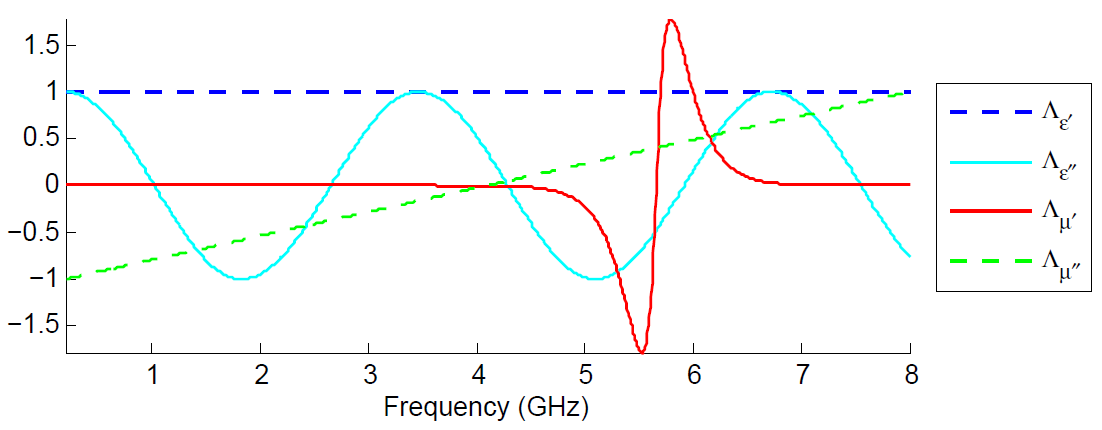
At each frequency $f$, the true (unknown) vector $\mathbf{x}_{\mbox{true}}(f)$ is $4N=76$-dimensional, where:

• -

  $\mathbf{x}_{\mbox{ref}}(f)$ is a reference frequency profile, depending on the area and on the radioelectric component ($\epsilon^{\prime},\epsilon^{\prime\prime},\mu^{\prime},\mu^{\prime\prime}$). Note that these $4N_{a}=20$ reference profiles are chosen regular and with typical orders of magnitude (i.e. non-negative and $\leq 20$).

• -

  $\Lambda(f)$ is a perturbation function depending on the radioelectric component. Thus, the $4$ functions $\Lambda_{\epsilon^{\prime}},\Lambda_{\epsilon^{\prime\prime}},\Lambda_{\mu^{\prime}},\Lambda_{\mu^{\prime\prime}}$ define the perturbation shapes . As shown in figure 9, they are chosen more or less regular (in order to test the inversion capabilities).

• -

  $c$ is a simple scaling factor, depending on the area. To examine the perturbation amplitude influence, increasing values of $c$ are chosen: $\{0.5,1,2,4,8\}$, related to the $5$ successiveareas.

According to the conventional RCS acquisition mode described in section 2.1, complex scattering coefficients are measured for both polarizations HH and VV, at $K_{f}=20$ regularly spaced frequencies ($f_{1}=0.2\;\mbox{GHz},\cdots,f_{K_{f}}=8\;\mbox{GHz}$) and at $K_{\theta}=23$ regularly spaced incidence angles ($\theta_{1}=0^{\circ},\cdots,\theta_{K_{\theta}}=180^{\circ}$).

The observation data $\mathbf{y}=(\mathbf{y}_{1},\ldots,\mathbf{y}_{K_{f}})$ is simulated from the likelihood model (2). That involves to run the parallelized harmonic Maxwell solver ($\mathcal{F}_{\mathrm{Maxwell}}$) and to draw an additive white Gaussian noise of marginal standard deviation $\sigma_{\mathrm{n}}=10^{-3}$ ($\sim$ $1\%$). Note that each of the $20$ observation vectors $\mathbf{y}_{k}$ is $4\times K_{\theta}=92$-dimensional. The data is represented in figure 10. Note on the amplitude representations the high specular reflections when the ogival object is turned perpendicularly to the wave propagation direction.

The state space dimension stems from the wave frequency number and from the discretization of the object in elementary mesh zones. In order to limit it, the cutting up of the object is here restricted to $N=19$ elementary zones.

The prior information (see section 3) needs to be detailed in this context. Concerning the prior spatial information $p(\mathbf{x}_{k})$, its means $\mathbf{m}_{k}$ are given, for each $k$, by the former reference frequency profiles $\mathbf{x}_{\mbox{ref}}(f_{k})$. Around them, the uncertainties are given by the block-structured covariance matrices $\mathbf{P}_{k}$ of (9) with: $\rho_{S}=0.95$ and $\sigma_{k}(i)=1+0.15\times\mathbf{m}_{k}(i)$ for any elementary zone $i$. In other words, we assume a minimum standard deviation of $1$ that increases proportionally to the reference amplitude value. Regarding the prior frequential information, we assume that $\rho$ depends on both area and EM property ($\epsilon^{\prime},\epsilon^{\prime\prime},\mu^{\prime},\mu^{\prime\prime}$), so that it is $20$-dimensional. As for its prior distribution $p(\rho)$, we set:

where all the marginal prior distributions $p(\rho_{i})$ are identical and presented on figure 11. Note that this distribution $p(\rho)$ can be sampled straightforwardly by sampling independently each component $\rho_{i}$ using, e.g., an acceptance/rejection method.

The surrogate likelihood model (7) has been formerly learned: $\mathbf{A}_{k}$ and $\mathbf{y}^{0}_{k}$ are known (see figure 6), as well as the marginal standard deviation $\sigma_{\mathrm{n}}$ which is in conformity with the measurement noise of the above observation simulation.

The sequence of probability measures $\eta_{n}$ is standardly defined by the annealed scheme (see section 4.3). To ensure a stable behavior of the SMC algorithm (i.e. keep a good approximation $\eta_{n}^{N_{p}}\simeq\eta_{n}$ until the end), we chose the following efficient adaptive strategies (that make it possible to limit the number of particles to $N_{p}=100$):

• -

  selection step: as mentioned, the increment ${\Delta\alpha}_{n}=\alpha_{n}-\alpha_{n-1}$ controls the selectivity degree. If ${\Delta\alpha}_{n}$ is too small, every particle is given approximately the same weight, and there is no selection among them. If ${\Delta\alpha}_{n}$ is too large, the majority of the particles are killed, the cloud loses all its diversity, and the SMC algorithm performs poorly. Therefore, instead of choosing beforehand ${\Delta\alpha}_{n}$, it is defined adaptively so that the selection step kills around $25\%$ of the particle population. This is a way to ensure a reasonable selection.

• -

  mutation step: the mutation step is crucial since it allows the particles to explore the state space $E$. We use Markov kernels $M_{n}$ defined as being the composition of several Metropolis-Hastings kernels $K_{n}^{(i)}$ whose proposition kernels $Q_{n}^{(i)}(x,dy)$ are uniform, centered in $x$, and associated with a window size $\sigma_{\mathrm{prop},n}^{(i)}$. To be sure that the particles move in a well-sized neighborhood, (i.e. large enough to explore $E$ and small enough to converge), the sequence $(\sigma_{\mathrm{prop},n}^{(i)})_{i}$ always starts with large values and decreases geometrically. Once more, we use an adaptive criteria to stop the process.

In the context of this reference study, the inversion process takes about $30$ minutes with a current standard processor. Note that the higher the dimension space is, the longer the inversion. In figure 12, we show the estimations of $\mu^{\prime}$ for all the zones of the object, with their associated uncertainties, compared with the true values, at a fixed frequency $f_{14}=5.6\;\mbox{GHz}$. Note that the EM property deviation is important in our example (see figure 9). As already mentioned, it is possible to provide some samples of the posterior distribution $p(\mathbf{x}_{14}|\mathbf{y})$ to determine the uncertainty on the estimators. The EM radioelectric properties are correctly inferred all along the ogival object and its 5 material areas. The uncertainty recovers more or less the real profiles.

Figure 13 presents frequential profiles for a fixed elementary zone (the $18^{\mathrm{th}}$). All the components ($\epsilon^{\prime},\epsilon^{\prime\prime},\mu^{\prime},\mu^{\prime\prime}$) are represented. Each of them is quite accurately estimated. The results are good, even when the perturbations (i.e. the difference between the prior and real profiles) are large and irregular. This robustness is due to the adaptive estimation of $\rho$’s components. Next it is confirmed by several thorough analysis.

References

- [1] KI Hopcraft and PR Smith. An introduction to electromagnetic inverse scattering. Kluwer Academic Publishers, 1992.
- [2] D. Colton, H. Haddar, and M. Piana. The linear sampling method in inverse electromagnetic scattering theory. Inverse problems, 19:S105, 2003.
- [3] E.F. Knott, J.F. Shaeffer, and M.T. Tuley. Radar cross section. SciTech Publishing, 2004.
- [4] R. Abbato. Dielectric constant measurements using RCS data. Proceedings of the IEEE, 53(8):1095–1097, 1965.
- [5] S. Coen. Inverse scattering of the permittivity and permeability profiles of a plane stratified medium. Journal of Mathematical Physics, 22:1127, 1981.
- [6] L. Garnero, A. Franchois, J.P. Hugonin, C. Pichot, and N. Joachimowicz. Microwave imaging-complex permittivity reconstruction-by simulated annealing. IEEE Transactions on Microwave Theory and Techniques, 39(11):1801–1807, 1991.
- [7] S. Caorsi, G.L. Gragnani, and M. Pastorino. Two-dimensional microwave imaging by a numerical inverse scattering solution. IEEE Transactions on Microwave Theory and Techniques, 38(8):981–980, 1990.
- [8] A. Ribes and F. Schmitt. Linear inverse problems in imaging. Signal Processing Magazine, IEEE, 25(4):84–99, 2008.
- [9] G. Demoment. Image reconstruction and restoration: Overview of common estimation structures and problems. IEEE Transactions on Acoustics, Speech and Signal Processing, 37(12):2024–2036, 1989.
- [10] F. Collino, M.B. Fares, and H. Haddar. Numerical and analytical studies of the linear sampling method in electromagnetic inverse scattering problems. Inverse Problems, 19:1279, 2003.
- [11] P. Del Moral, A. Doucet, and A. Jasra. Sequential Monte Carlo for Bayesian computation. Bayesian Statistics, 8(1):34, 2007.
- [12] S. Geman and D. Geman. Stochastic relaxation, Gibbs distributions, and the Bayesian restoration of images. IEEE Transactions on Pattern Analysis and Machine Intelligence, (6):721–741, 1984.
- [13] M.C. Robini, T. Rastello, and I.E. Magnin. Simulated annealing, acceleration techniques, and image restoration. IEEE Transactions on Image Processing, 8(10):1374–1387, 1999.
- [14] A.D. Lanterman. Statistical radar imaging of diffuse and specular targets using an expectation-maximization algorithm. In SPIE Proceedings, pages 20–31. Citeseer, 2000.
- [15] M. Pastorino. Stochastic optimization methods applied to microwave imaging: A review. IEEE Transactions on Antennas and Propagation, 55(3):538–548, 2007.
- [16] E. Michielssen, J.M. Sajer, S. Ranjithan, and R. Mittra. Design of lightweight, broad-band microwave absorbers using genetic algorithms. IEEE Transactions on Microwave Theory and Techniques, 41(6):1024–1031, 1993.
- [17] B. Chambers and A. Tennant. Optimised design of radar absorbing materials using a genetic algorithm. In IEE Radar, Sonar and Navigation Proceedings, volume 143, pages 23–30. IET, 1996.
- [18] J.S. Liu and R. Chen. Sequential Monte Carlo methods for dynamic systems. Journal of the American statistical association, pages 1032–1044, 1998.
- [19] P. Minvielle, E. Tantar, A. Tantar, and P. Berisset. Sparse antenna array optimization with the cross-entropy method. IEEE Transactions on Antennas and Propagation, 59(8):2862–2871, 2011.
- [20] D.R. Wehner. High resolution radar. Norwood, MA, Artech House, Inc., 1995, 1995.
- [21] A.C. Woo, H.T.G. Wang, M.J. Schuh, and M.L. Sanders. EM programmer’s notebook-benchmark radar targets for the validation of computational electromagnetics programs. Antennas and Propagation Magazine, IEEE, 35(1):84–89, 1993.
- [22] B. Stupfel, R. Le Martret, P. Bonnemason, and B. Scheurer. Combined boundary-element and finite-element method for the scattering problem by axisymmetrical penetrable objects. Mathematical and numerical M, 2:78–17, 1991.
- [23] IEEE Recommended Practice for Radar Cross-Section Test Procedures. IEEE Std 1502-2007, pages 1 –60, 7 2007.
- [24] P. Del Moral. Feynman-Kac formulae. Genealogical and interacting particle approximations. Springer New York, 2004.
- [25] O. Cappé, E. Moulines, and T. Rydén. Inference in hidden Markov models. Springer Series in Statistics. Springer, New York, 2005.
- [26] A. Doucet, N. De Freitas, and N. Gordon. Sequential Monte Carlo Methods in Practice. Springer New York, 2001.
- [27] P. Del Moral. Nonlinear filtering: Interacting particle solution. Markov Processes and Related Fields, 2(4):555–579, 1996.
- [28] F. Cérou, P. Del Moral, T. Furon, and A. Guyader. Sequential Monte Carlo for rare event estimation. Stat. Comput., 22(3):795–808, 2012.
- [29] P. Del Moral, A. Doucet, and A. Jasra. Sequential Monte Carlo Samplers. Journal of the Royal Statistical Society, Series B, 68:411–436, 2006.
- [30] P. Del Moral and A. Guionnet. On the stability of interacting processes with applications to filtering and genetic algorithms. Annales de l’Institut Henri Poincaré, 37(2):155–194, 2001.
- [31] A. Jasra, D.A. Stephens, and C.C. Holmes. On population-based simulation for static inference. Statistics and Computing, 17(3):263–279, 2007.